Detection of a dense group of hyper-compact radio sources in the central parsec of the Galaxy

Abstract

Using the JVLA, we explored the Galactic center (GC) with a resolution of 0.05” at 33.0 and 44.6 GHz. We detected 64 hyper-compact radio sources (HCRs) in the central parsec. The dense group of HCRs can be divided into three spectral types: 38 steep-spectrum ($\alpha\leq-0.5$) sources; 10 flat-spectrum ($-0.5<\alpha\leq 0.2$) sources; and 17 inverted-spectrum sources having $\alpha>0.2$, assuming $S\propto\nu^{\alpha}$. The steep-spectrum HCRs are likely represent a population of massive stellar remnants associated with nonthermal compact radio sources powered by neutron stars and stellar black holes. The surface-density distribution of the HCRs as function of radial distance ($R$) from Sgr A* can be described as a steep power-law $\Sigma(R)\propto\/R^{-\Gamma}$, with $\Gamma=1.6\pm 0.2$, along with presence of a localized order-of-magnitude enhancement in the range 0.1-0.3 pc. The steeper profile of the HCRs relative to that of the central cluster might result from the concentration massive stellar remnants by mass segregation at the GC. The GC magnetar SGR J1745-2900 belongs to the inverted-spectrum sub-sample. We find that two spectral components present in the averaged radio spectrum of SGR J1745-2900, separated at $\nu\sim 30$ GHz. The centimeter-component is fitted to a power-law with $\alpha_{cm}=-1.5\pm 0.6$. The enhanced millimeter-component shows a rising spectrum $\alpha_{mm}=1.1\pm 0.2$. Based on the ALMA observations at 225 GHz, we find that the GC magnetar is highly variable on a day-to-day time scale, showing variations up to a factor of 6. Further JVLA and ALMA observations of the variability, spectrum, and polarization of the HCRs are critical for determining whether they are associated with stellar remnants. Unified Astronomy Thesaurus concepts: Center of the Milky Way; [Galactic center (565)]; Interstellar medium (847); Radio continuum emission (1340); Black holes (162); Pulsars (1306); Magnetars (992); Neutron stars (1108); Discrete radio sources (389); Radio transient sources (1358); Radio interferometry (1346)

1 Introduction

One of the outstanding open questions that has challenged astronomers for many years is the “missing pulsar problem”: there are far fewer pulsars found toward the Galactic center (GC) than we could expect, given the formation rate of massive stars in the central molecular zone of the Galaxy implied by the relative abundance of massive stars produced at the GC over the past ten million years (e.g., Dong, Wang & Morris., 2012; Lu et al., 2013; Clark et al., 2021). This can in part be ascribed to the large foreground scatter-broadening at longer radio wavelengths toward the GC, which can lead to a large enough pulse broadening that the pulses become indistinguishable (Lazio & Cordes, 1998). Several other reasons also complicate the discovery of GC pulsars, as detailed by Eatough et al. (2021). However, the discovery of a magnetar associated with SGR J1745-2900, located just 3” from Sgr A* (Kennea et al., 2013; Mori et al., 2013; Rea et al., 2013), indicates that the effect of the scattering screen could be up to three orders of magnitude smaller than had previously been expected (Spitler et al., 2014; Bower et al., 2014). Consequently, the question remains: why haven’t more pulsars been seen toward the Galactic center? Because massive stars clearly form in abundance at the GC, and because dynamical friction should cause the more massive stellar remnants to be concentrated there, neutron stars should be abundant and continuously produced in the GC region ($R\sim 0.5$ pc) (Bahcall & Wolf, 1976; Morris, 1993; Miralda-Escudé & Gould, 2000; Pfahl & Loeb, 2004; Alexander & Hopman, 2009; Merritt, 2010; Antonini & Merritt, 2012; Alexander et al., 2017).

One obvious answer to this question of where the pulsars are is that the number of “windows” in the scattering screen is quite small, so that most pulsars are still too scatter-broadened for their pulses to be detected at the wavelengths searched. Another, perhaps more interesting answer is that massive stars that form out of the rather highly magnetized interstellar medium of the GC (Morris, 2014) tend to themselves be rather strongly magnetized, and therefore leave strongly magnetized neutron star remnants. That is, pulsars formed near the GC could frequently be magnetars, which have short lifetimes as recognizable pulsars ($\sim 10^{3}-10^{5}$ yrs) because of their rapid spin-down rates (Harding et al., 1999; Espinoza et al., 2011; Kaspi & Beloborodov, 2017). Such short lifetimes would limit the number of pulsars that could be detected at any one moment to a small number, although they could remain detectable as compact radio sources. Radio continuum surveys of point sources can help distinguish these possibilities. We recently published a 5.5-GHz survey of GC compact radio sources (GCCRs) within a radius of $\sim$7.5 arcmin (17 pc) of Sgr A* (Zhao, Morris & Goss, 2020), and concluded that, of the 110 new compact radio sources observed down to a 10-$\sigma$ sensitivity limit of 70 $\mu$Jy, most of them fall within the high flux density tail of normal pulsars at the GC (our effort to decrease the 5.5-GHz flux density limit with existing, additional data is in progress). Of course, there are several other possible assignations for these sources; 82 of them are variable or transient and 42 have possible X-ray counterparts.

Limited by the VLA angular resolution and confusion from the HII continuum emission from Sgr A West, the 5.5-GHz survey focussed primarily on regions lying beyond a radius of R $\sim$ 1 pc from Sgr A*, that is, on regions outside the circumnuclear disk. To take the next step in addressing the pulsar puzzle, we have recently surveyed the central $\pm$0.5 parsecs ($\pm$13”) around Sgr A* at higher frequencies, using existing JVLA Ka and Q-band data and X-band observations in the A-array. The high-resolution JVLA observations at 33 and 44.6 GHz were used to search for hyper-compact (¡ 0.1”) radio sources (HCRs) in Sgr A West, and to study their radio properties and distribution near Sgr A*. The motivation for going to higher frequencies in the context of constraining the magnetar population comes from the discovery by Torne et al. (2017) that the spectrum of the magnetar near Sgr A*, SGR J1745-2900, rises at higher frequencies to a millimeter/submillimeter plateau. Another magnetar, 1E 1547.0$-$5408, has also been seen to display a spectrum rising at millimeter wavelengths (Chu et al., 2021). If such a rising spectrum happens to be a general characteristic of magnetars, then this feature can be used to identify magnetar candidates with higher frequency observations, even if radio pulses are not detectable.

This paper is organized as follows: Section 2 describes the JVLA observations, data reduction and imaging procedures used for identifying HCRs within the central parsec. We also describe there our procedure for data reduction and imaging using archival ALMA data for measurements of SGR J1745-2900. Section 3 presents a catalog of the HCRs found within Sgr A West. Three selected cases of HCRs are described in Section 4, including detailed results on the radio spectrum and variability of the GC magnetar SGR J1745-2900, based on data from this paper and from prior publications. Section 5 shows a statistical analysis of HCRs by dividing them into three spectral types. Possible origins of the HCRs as well as massive stellar remnants as a consequence of the mass segregation in the central parsec are also discussed in section 5. Finally, section 6 summarizes our conclusions.

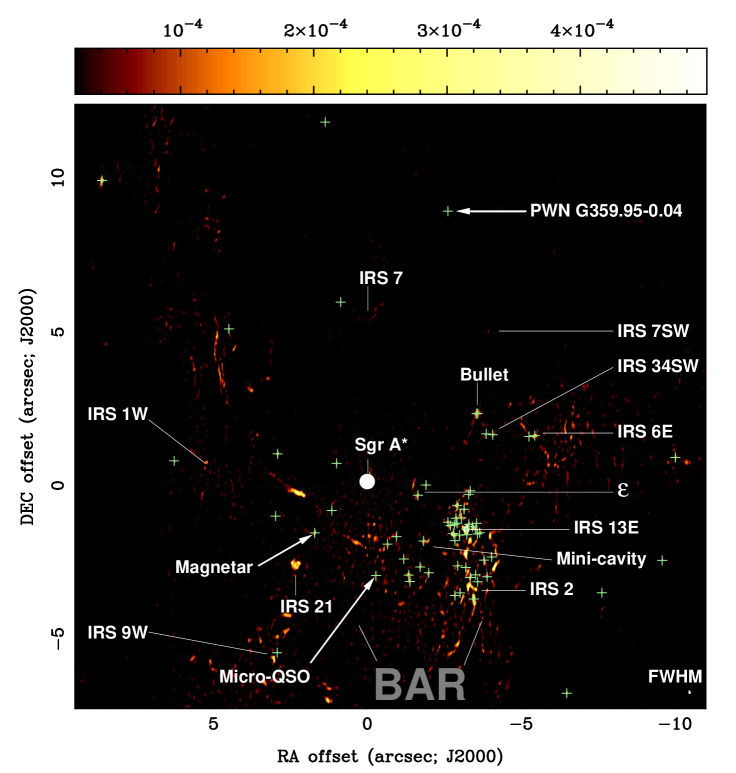
Figure 1: Ka-band image of the central 0.8 parsec of the Galaxy. Sgr A* is indicated as a white filled circle, and all 64 HCRs that we have identified in this region are marked with green crosses. This 33-GHz image was made with baselines from 500 to 4,000 k$\lambda$, giving a FWHM beam of 0.08$\times$0.03” and an rms noise of 8 $\mu$Jy beam^-1. The color wedge scales intensity in units of Jy beam^-1. In addition to the marked HCRs, some extended features corresponding to fine-scale structures in the Northern Arm, Eastern Arm, and the “mini-cavity” of the Sgr A West HII region, which are present in this image, are also labelled. The position of Sgr A* is registered at RA(J2000)=17:45:40.0409, Dec(J2000)= $-$29:00:28.118 (Reid & Brunthaler, 2014) in the equatorial coordinate system.

Table 1: Log of JVLA datasets and images

	UV data							Images
Project ID	Array	Band	$\nu$	$\Delta\nu$	$\Delta t$	HA range	Epoch	Weight	($\theta_{\rm maj}$,$\theta_{\rm min}$, ${\rm PA}$)	rms
			(GHz)	(GHz)		(sec)	(day)	(R)	(arcsec, arcsec, deg)	($\mu$Jy beam-1)
(1)	(2)	(3)	(4)	(5)	(6)	(7)	(8)	(9)	(10)	(11)
15A-293	A	Q†	44.6	8	3	$-0^{h}.6$ — $+2^{h}.5$	2015-09-16	0	0.078, 0.032, 12	17
…	…	Ka†	33.0	8	2	$-2^{h}.8$ — $+0^{h}.3$	2015-09-11	$-$0.3	0.079, 0.031, $-11$	8
14A-346	A	X‡	9.0	2	2	$-3^{h}.4$ — $+3^{h}.3$	2014-04-17	0	0.36, 0.15, $-6$	4
19B-289	A	X‡	9.0	2	2	$+0^{h}.6$ — $+2^{h}.6$	2019-09-21	0	0.36, 0.15, $-6$	7
20B-203	A	X‡	9.0	2	2	$-0^{h}.3$ — $+2^{h}.9$	2020-11-20	0	0.36, 0.15, $-6$	5
…	…	…	…	…	…	$-1^{h}.5$ — $+1^{h}.7$	2020-12-04	…	…	…

(1) JVLA program code of PI: Mark Morris for 19B-289 and 20B-203; PI: Farhad Yusef-Zadeh for 14A-346 and 15A-293. (2) Array configurations. (3) JVLA band code; ”X”,”Ka”, and ”Q” stand for the VLA bands in the ranges of $8.0-12.0$ GHz, $26.5-40.0$ GHz and $40.0-50.0$ GHz (https://science.nrao.edu/facilities/vla/docs/manuals/oss2013B/performance/bands). (4) observing frequencies at the observing band center. (5) bandwidth. (6) integration time. (7) hour angle (HA) range for the data. (8) date corresponding to the image epoch. (9) robustness weight parameter. (10) FWHM of the synthesized beam. (11) rms noise of the image. †Correlator setup: 64 channels in each of 64 subbands with channel width of 2 MHz ‡Correlator setup: 64 channels in each of 16 subbands with channel width of 2 MHz.

2 Observations, data & imaging

Following the 5.5 GHz JVLA A-array survey of compact radio sources within a radius of 7.5 arcmin (17 pc) in the Galactic center region, we have carried out a search for compact radio sources within a radius of 13” (0.5 pc) based on the existing JVLA high-resolution data at 44.6 GHz (Q-band) and 33.0 GHz (Ka-band) as well as our recent JVLA A-array observations at 9 GHz. The high-resolution and sensitive VLA observations at high radio frequencies are crutial in detections of HCRs at a level of 100 $\mu$Jy to a few mJy in the vicinity of Sgr A*.

2.1 JVLA data, calibration & imaging

New JVLA observations in the A configuration were carried out on 2019-9-21, 2020-11-20 and 2020-12-4 at 9 GHz, in addition to the observation on 2014-04-17 that was used to image the Sgr A West filament (Morris et al., 2017). The X-band observations were all carried out with the VLA standard correlator setup for wideband continuum covering 2 GHz bandwidth, produced from the 8-bit sampler. We also acquired the higher-resolution NRAO archival data observed with the JVLA in the A-array at 33 and 44.6 GHz on 2015-9-16 and 2015-9-11, respectively. The Q- and Ka-band observations were using the 3-bit sampler, producing 64 subbands and covering a total of 8 GHz bandwidth. All the observations were pointed at a sky position, very near Sgr A*. Table 1 summarizes the six sets of uv data (columns 1 - 8). The data reduction was carried out using the CASA software package of the NRAO. The standard calibration procedure for JVLA continuum data was applied. 3C 286 (J1331+3030) was used for corrections for delay, bandpass and flux-density scale.

J1733-1304 (NRAO 530) and J1744-3116 were used for complex gain calibrations. In addition, corrections for the time variation of the bandpass across each baseband due to residual delays were determined using NRAO 530 based on the model discussed in Zhao, Morris & Goss (2019) . The accuracy of the flux-density scale at the JVLA is 3%$-$5%, limited by the uncertainty of the flux density of the primary calibrator, Cygnus A (Perley & Butler, 2017). Following the procedure for high dynamic range (DR) imaging that we developed recently (Zhao, Morris & Goss, 2019) and applying it to the Sgr A data with CASA, we further corrected for the residual errors in phase. The integration time of the calibrated Q and Ka-band data was averaged into 30-sec time bins, so that the intensity loss at the 13” outer radius of the search region is less than 10% due to the smearing effect caused by the Earth’s spin. After correcting for the residual delay, we also binned the spectral channel data to channel widths of 32 and 16 MHz for the Q- and Ka-band data, respectively, to ensure that the intensity loss for a point source caused by bandwidth smearing is less than 10% at the radius of 13”. The short baseline data ($<500{\rm k}\lambda$) were filtered out in order to avoid contamination by the extended emission in Sgr A West on scales $>0.4$”. The Ka-band image shown in Fig. 1 is made with CASA task $CLEAN$ from the baseline data between 500-4,000 k$\lambda$, achieving an rms of 8 $\mu$Jy beam^-1 with a FWHM beam of 0.079”$\times$0.031 ($-11^{\rm o}$). This high-resolution image shows numerous compact radio sources in the central parsec region.

For the X-band data, after corrections for the residual errors, the visibility data were averaged to a time bin of 16 sec while the original channel width of 2 MHz was kept. We made images at 9 GHz using the multi-frequency synthesis algorithm (MFS: Rau & Cornwell, 2011) with the 1024 spectral channels covering the 2 GHz bandwidth. Also we filtered out the short baselines ($<100$ k$\lambda$), and constructed two 9-GHz images for both the 2019 and 2020 epochs. The second epoch image was made with the two observations on 2020-11-20 and 2020-12-04. Hereafter, we use the mean epoch, 2020-11-27, for this image. The rms noise for the 2020-11-27 X-band image is 5 $\mu$Jy beam^-1. We reconstructed the 2014-04-17 image with the calibrated X-band A-array data (Morris et al., 2017) by using only the long-baseline data ($>100$ k$\lambda$). The rms noise for the resulting 2014-04-17 X-band image is 4 $\mu$Jy beam^-1.

The specified parameters for the final images at Q-, Ka- and X-bands are summarized in Table 1 from columns 9 to 11.

2.2 ALMA data, calibration & imaging

We acquired archival data from the Atacama Large Millimeter Array (ALMA), observed by Tsuboi et al. (2019) at 225.75 GHz in Cycle 5 (2017.1.00503.S). Following the ALMA CASA guide for Cycle 5 data reduction, we executed the pipeline script “scriptForPI.py” to produce calibrated ALMA data in CASA Measurement Set format. The ALMA datasets are composed of ten 1-hr observations of IRS 13E in the array configuration of C43-10 within a two-week interval between 2017-10-6 and 2017-10-20. The observing field covers Sgr A* and the magnetar SGR J1745-2900 in addition to IRS 13E. The pipelined ALMA images appear to be marred by severe residual errors. Both IRS 13E and SGRA J1745-2900 were buried in the sidelobes and artifacts produced by the residual dirty beam. Then, following the recipe for dynamic range imaging with wideband data (Zhao, Morris & Goss, 2019), we corrected the residual errors by utilizing the antenna-based closure relations (Thompson, Moran & Swenson, 2017) and constructed a refined ALMA image from the data observed at the first epoch on 2017-10-6 as a trial case using CASA task $tCLEAN$ with the MFS algorithm and robust weighting with Briggs parameter R=0 (Briggs, 1995). An rms noise of $\sigma=20\leavevmode\nobreak\ \mu$Jy beam^-1 was achieved, with a FWHM beam of 0.024”$\times$0.017” (82^o). The magnetar SGR J1745-2900 was successfully detected with a S/N ratio of 70. We then made 2D-Gaussian fits to both Sgr A* and the magnetar, finding flux densities of 3.031$\pm$0.013 Jy and 1.41$\pm$0.08 mJy at 225 GHz for Sgr A* and the magnetar, respectively. Fig. 2a shows the ALMA continuum image of the magnetar at 225.75 GHz. Based on the procedure and input parameters for the CASA tasks that were used for the trial case, we coded the detailed CASA reduction steps for the ALMA data into a CASA-Python script. Using this script for corrections of residual errors, we further processed the datasets from all ten epochs observed on 2017-10-6, 2017-10-7, 2017-10-9, 2017-10-10, 2017-10-11, 2017-10-12, 2017-10-14, 2017-10-17, 2017-10-18, and 2017-10-20. The flux densities for the magnetar were determined by fitting a 2D-Gaussian and are tabulated in Table 3 (see Section 4).

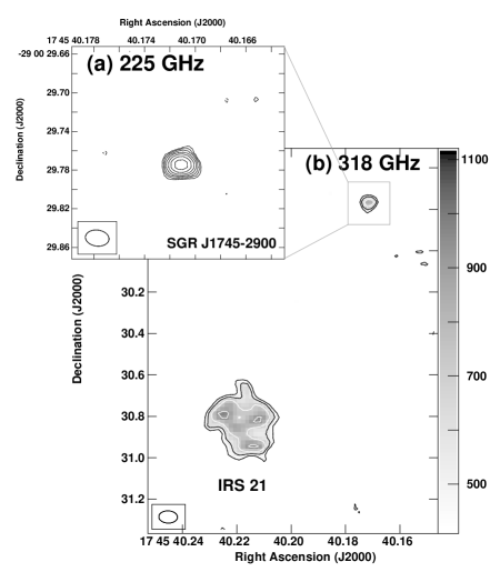
Figure 2: (a) Contour image of the magnetar SGR J1745-2900 observed on 2017-10-6 using ALMA at 225.75 GHz with a FWHM beam of 0.024”$\times$0.017” (PA 82^o). Contours are $\sigma_{\rm im}\times$($-$5.7, 5.7, 8, 11.3, 16, 22.6, 32, 45.3 ), where $\sigma_{\rm im}=22\mu$Jy beam^-1. (b) ALMA image of the magnetar SGR J1745-2900 (top-right: a point source) and IRS 21 (bottom-left: a complex) observed on 2019-10-14 at 318 GHz with a FWHM beam of 0.087”$\times$0.059” (89.5^o). Contours are $\sigma_{\rm im}\times$($-$6, 6, 8, 11, 15), where $\sigma_{\rm im}=55\mu$Jy beam^-1. The FWHM beams are illustrated at the bottom-left corner in each image. Numbers on the grey scale bar are in units of $\mu$Jy beam^-1.

We also re-processed ALMA archival data (2015.1.01080.S) for observations at 343.49 GHz by Tsuboi et al. (2017). The observations were carried out at four epochs 2016-4-23, 2016-8-30, 2016-8-31 and 2016-9-8, for durations of 3h, 1h, 2h and 3h, respectively. The 2016-4-23 observation was in the C36-2/3 array configuration, and other three observations were in the C40-6 configuration. The pipeline-calibrated datasets were obtained by executing the pipeline script “scriptForPI.py”. We then adjusted the input parameters in the CASA-Python script used for imaging the 225-GHz data, and applied the script to the 343-GHz data. The spatial resolution of the first 343-GHz image from epoch 2016-4-23 is relatively poor, with FWHM beam of 0.35”$\times$0.33” ($-79^{\rm o}$), and the emission from the magnetar SGR J1745-2900 appears to be contaminated by surrounding extended emission. The final image of SGR J1745-2900 was made by applying a high-pass baseline filter, so that only long-baseline data were included (${\rm>100\leavevmode\nobreak\ k\lambda}$), thus filtering out extended ($>2$”) emission features. An rms noise of 13 mJy beam^-1 was achieved for the epoch 2016-4-23, and the flux density of 3.29$\pm$0.34 mJy was determined for the magnetar at 343 GHz. The observations from the later epochs at 343 GHz have a typical angular resolution of 0.1”. The rms noise values were 0.15, 0.05 and 0.12 mJy beam^-1 for the 2017-8-30, 2017-8-31 and 2017-9-8 images, respectively. The magnetar SGR J1745-2900 is detected in all four epochs at 343-GHz, and the flux densities are determined at a level of 10$\sigma$ or better using 2D-Gaussian fitting. The measurements are reported in Table 3, including a 5% error in the flux-density calibration (Bonato et al., 2018).

A high-resolution (0.087”$\times$0.059”, PA = 89.5^o) ALMA observation was carried out at 320 GHz in the C43-6 array configuration on 2019-10-14 (2018.A.00052.S of P.I. Mark Morris). The data was initially processed with the pipeline script “scriptForPI.py”. Subsequently, we made further corrections for the residual errors with the CASA-Python script described above and then imaged the region containing the GC magnetar, Sgr A*, and IRS 21 with the two lower-frequency sub-bands centered at 318 GHz, which have relatively stable phase and less contaminations from molecular lines in the circumnuclear disk (CND). An rms noise of 55 $\mu$Jy beam^-1 was achieved. The magnetar is significantly detected with a flux density of 1.32$\pm$0.15 mJy. The uncertainties include a 5% error in the determination of the flux-density scale for ALMA observations. Fig. 2b shows the 318-GHz image of the region containing SGR J1745-2900 and IRS 21.

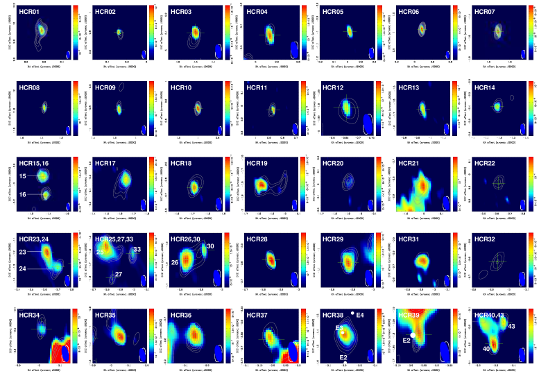
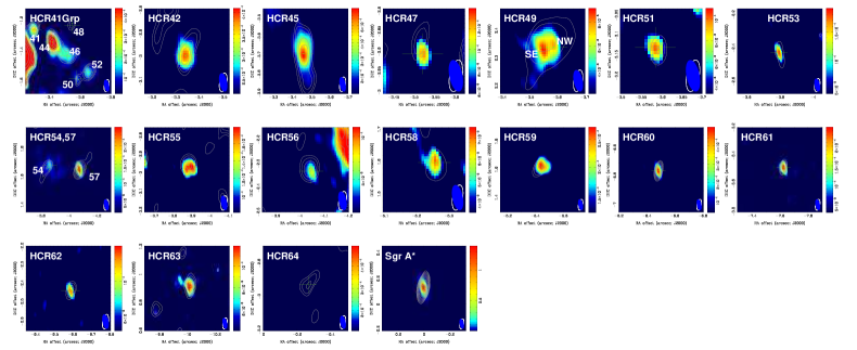
Figure 3: Images of individual HCRs, color for 44.6 GHz intensity and contours for 33 GHz from an image made with a long baseline filter of $>500\leavevmode\nobreak\ {\rm k}\lambda$ except for HCR39 which was made with a longer baseline filter $>1000\leavevmode\nobreak\ {\rm k}\lambda$ to separate the point-like source from the contamination of the extended emission associated with the radio core IRS 13E. The IR stars (E2, E3, and E4) detected in the IRS 13E region (Zhu et al., 2020) are marked with white dots (see HCR38 and HCR39 panels). The color wedges scale the intensity of 44.6-GHz emission in units of Jy beam^-1. The contours are $\sigma_{\rm im}\times 2^{\rm n/2}$ where n starts from $\rm n_{1}$ until reaching the source peaks. The values of $\sigma_{\rm im}$ and $\rm n_{1}$ corresponding to the individual HCR image panels are listed in Column 11 of Table 2. Bottom-right corners are the FWHM beams at 44.6 and 33 GHz: 0.08”$\times$0.03” (PA = 12^o) in blue and 0.08”$\times$0.03” (PA = -11^o) in white, respectively.

3 Hypercompact radio sources

3.1 Search procedure and selection criteria

The angular resolutions of the A-array observations at Ka- and Q-bands, 0.05”, are nearly two orders of magnitude smaller in beam area than the 5.5-GHz beam used in our previous study of the GCCRs (Zhao, Morris & Goss, 2020). At such a high spatial resolution, most of the emission components in the Sgr A West HII region have been resolved out. The emission from the HII sources produced overwhelming confusion at 5.5 GHz, which was the main issue preventing us from unambiguously detecting GCCRs in Sgr A West, given the relatively low angular resolution of 0.5”. The Ka-band JVLA, with both its superior angular resolution and sensitivity ($\sim 8\leavevmode\nobreak\ \mu$Jy beam^-1), is well suited for significant detection of point-like hyper-compact radio sources (HCRs) at a level of $>$0.1 mJy. Thus, we have an unprecedented opportunity for study of the compact radio sources associated with massive stellar remnants, such as pulsars, magnetars and accreting compact stellar remnants. Unlike the free-free emission of the HII components, the radio emission from such objects is expected to be nonthermal. Our search has therefore been focused on using the Ka- and Q-band images to identify nonthermal HCRs within the Galaxy’s central parsec. We proceeded in three steps as follows:

(1) We initially found approximately a thousand compact radio sources having angular size of $\lesssim 0.5$” based on a Ka-band image constructed including all baselines with a robust weighting parameter, R=0.25 (Briggs, 1995), and a FWHM beam of 0.12”$\times$0.06” (PA = $-11^{\rm o}$). A sensitivity threshold of S${}_{\rm 33\/GHz}$/$\sigma_{\rm rms}$ ¿ 6, $\sigma_{\rm rms}\approx 7\leavevmode\nobreak\ \mu$Jy beam^-1, was applied in the initial search. Bright intensity maxima in the HII emission components might have been included in the compact-source sample, producing false detections for the nonthermal compact radio sources. To ensure that the ultimate sample contains only compact nonthermal radio sources, two further steps were carried out:

(2) The Ka-band image was reconstructed with a robust weight R=$-$0.3 to down-weight the contribution from short baselines and also a high-pass baseline filter ($>500$ k$\lambda$) was applied. So we can separate point-like sources from extended emission. The final cleaned image was convolved with a beam having FWHM = 0.08”$\times$0.03” (PA = $-11^{\rm o}$), similar to the synthesized beam of the Q-band observations, but keeping the position angle of the Ka-band synthesized beam determined by the uv-data sampling. We narrowed the list for those sources that are detected at Ka-band by keeping only those sources above a S₃₃/$\sigma_{\rm rms}=15$ threshold and limiting the size of the major axis to be less than 0.1 arcsec ($\theta_{\rm maj}<0.1$”) based on a 2D Gaussian fitting. The number of candidates in the list was thereby reduced to $\sim$100. The remaining sub-sample only contains the hyper-compact members of the initial sample.

(3) Finally, we used the high-resolution Q-band image, with $\sigma_{\rm rms}=17\leavevmode\nobreak\ \mu$Jy beam^-1, FWHM = 0.08”$\times$0.03” (PA = 12^o), to narrow down the list of HCRs by imposing a conservative limit of $S_{44.6}/\sigma_{\rm im}>10$ on the detection significance and an upper limit on the positional offset between Ka- and Q-band positions less than $3\sigma$, where $\sigma$ is given in Table 2 with a typical value of a few milli-arcsec (mas), based on 2D-Gaussian fits at the two frequencies. We note that the locations of HII peaks depend on the uv-sampling. The uv data in the Q-band observations were primarily sampled in a positive hour-angle range while the Ka-band data were sampled in a negative hour-angle range. Consequently, the sources having a significant offset between the Q- and Ka-band images are suspected to be HII peaks and are therefore rejected from the HCR sample.

The equal beam sizes of the Q- and Ka-band images allow us to determine reliable spectral indices that will be used to further distinguish the source types. We do not use spectral indices as a selection parameter for the HCRs, given a wide range of values for the spectral indices covered by the radio sources associated with pulsars, magnetars and stellar-mass black holes. We note that the primary 15$\sigma$ significance cutoff used for Ka-band sources and the lower 10$\sigma$ cutoff for Q-band were chosen for the derivation of significant spectral indices, given the poorer sensitivity of the Q-band data. Neglecting fitting errors, for a weak point-like source, we expect a maximum uncertainty of $\sigma_{\alpha}\sim 0.4$ in spectral index.

Those candidates having consistent results from the Gaussian fitting to the Ka- and Q-band images were included in the final sample of HCRs, consisting of 64 members. We note that the conservative search criteria for HCRs may miss highly variable and relatively weaker sources having a steep spectrum, given that the sensitivity of Q-band observations is a factor of 2 poorer than that of Ka-band data. For example, a hyper-compact radio source in the IRS 7SW region (see Fig. 1) was rejected from the HCR sample because its Ka-band flux density below the 15$\sigma$ threshold.

In short, from the JVLA A-array images observed at 33 and 44.6 GHz on 2021-9-11 and 2021-9-11, we have identified 64 hyper-compact radio sources (HCRs) located inside Sgr A West within a radius of $13"$ from Sgr A* based on their compactness (a size of $\theta_{\rm maj}<0.1$”) at a conservative significance level of $S/\sigma>15$ at 33 GHz and $S/\sigma>10$ at 44.6 GHz. Three exceptions which were not detected at 44.6 GHz on 2015-9-16 are also included: HCR22, HCR32 and HCR64. HCR22 appears to be a strong candidate for the object that powers the X-ray PWN G359.95-0.04 (see Sec.4.1). HCR64 is a compact transient radio source associated with the microquasar discovered during the 2005 outburst of the X-ray transient XJ174540.0290031 (Muno et al., 2005; Porquet et al., 2005; Bower et al., 2005; Zhao et al., 2009); further discussion of this source is given in Sec.4.2. HCR32 appears to be a highly variable source. It was detected with a flux density of 0.5$\pm$0.1 mJy at 9 GHz at the epoch of 2014-4-17 but no significant detections were made in the 2019 and 2020 epochs at 9 GHz.

One of the sources, HCR49, is associated with the high-velocity head-tail radio/IR source designated the ”Bullet” (Yusef-Zadeh et al., 1998; Zhao & Goss, 1998; Zhao et al., 2009); it now appears to consist of at least two compact components.

3.2 Images of hyper-compact radio sources

Fig. 3 shows the images of all 64 HCRs in individual panels labelled with the HCR identification numbers, the colored images represent the 44.6-GHz HCRs and the superimposed contours are for the 33-GHz images made with baselines exceeding $500{\rm k\lambda}$. For those panels containing more than one HCRs, each of the HCRs is labelled with its HCR ID. The green plus symbols mark the positions determined from the 44.6-GHz data. For HCR22, HCR32 and HCR64, which were not detected at 44.6 GHz, the 33-GHz positions are shown.

3.3 A catalog for hyper-compact radio sources

Table 2 lists 64 HCRs. Column 1 gives the ID numbers for the members of the HCR catalog. Columns 2 and 3 are the J2000 coordinates, omitting the common part of 17^h45^m in Right Ascension (RA) and $-29^{\rm o}$00’ in Declination (Dec). With the exception of HCR22, HCR32, and HCR64, the Q-band coordinates of the HCRs were determined with respect to Sgr A*’s equitorial coordinates at the J2000 epoch (Reid & Brunthaler, 2014). The positions of non-Q-band sources are determined using the Ka-band data. The 1$\sigma$ uncertainties in the last digits of RA and Dec. are given in parentheses. We note that, throughout this paper, the positions of the HCRs in the figures are labelled in the J2000 equatorial coordinate system with respect to the position of Sgr A*. Columns 4 and 5 list the flux densities at 44.6 and 33 GHz with 1$\sigma$ uncertainties. Columns 6, 7 and 8 show the source sizes, deconvolved from the telescope beam, including major ($\theta_{maj}$) and minor ($\theta_{min}$) axes, as well as the position angle (PA), all with their 1$\sigma$ uncertainties. Column 9 lists the spectral index, $\alpha$ ($S\sim\nu^{\alpha}$), determined from the flux densities at 44.6 and 33 GHz. The parameters used to plot the contours in Fig. 3 for individual HCRs are listed in Column 10: $\sigma_{\rm im}$ representing the rms variations of the background regions near the sources and ${\rm n_{1}}$ being the integer corresponding to the multiplicative factor, $2^{0.5n}$, specifying the lowest contour. Column 11 gives a brief note on individual HCRs.

Finally, we examined the HCRs that can be spatially associated with the 7mm-IR(3.8$\mu$m) sources (Yusef-Zadeh et al., 2014) by transfering their coordinates to the J2000 equatorial coordinate system used in this paper, in which Sgr A* is located at RA(J2000) = 17:45:40.0409, Dec(J2000) = $-$29:00:28.118 (Reid & Brunthaler, 2014). After corrections for the system errors (${\rm\Delta RA=0.0026^{\rm s}}$, ${\rm\Delta Dec=-0.049}$”) that mainly caused by the difference of the position of Sgr A* between Reid & Brunthaler (2014) and Yusef-Zadeh et al. (2014), 22 HCRs are identified with possible 7mm-IR sources within an uncertainty of 25 mas, the typical positional accuracy given for the 7mm-IR sources. The ID numbers of the possible 7mm-IR counterparts are given in Column 11 as well.

Figure 4: (a) The Ka-band image made with the JVLA A-array data using all available baselines, showing the radio structure of HCR22, a candidate source of particles and energy powering the PWN. The contours are 5 $\mu$Jy beam${}^{-1}\times$ ($-4$, 4, 5.7, 8, 11.3, 16) with FWMH = 0.11”$\times$0.04”, $-11^{\rm o}$ (bottom-right). (b) JVLA 9-GHz images at epochs 2014-4-17 (color) and 2020-11-27 (contours). The contours are 50 $\mu$Jy beam${}^{-1}\times$ (64, 80, 96, 112, 128) with FWMH = 0.36”$\times$0.15”, $-6^{\rm o}$ (bottom-right). The green plus marks the peak position at 33 GHz. The three black ellipses mark the peak positions of the counterpart at 9 GHz at the three observing epochs as labelled. The size of each ellipse scales the 1 $\sigma$ uncertainty of the peak position determined from a 2D-Gaussian fitting. The color wedge scales the intensity in units of Jy beam^-1 for the JVLA images. (c) The Chandra X-ray image (angular resolution = 0.5”, from Zhu et al., 2018) of the PWN G359.95-0.04 (Wang et al., 2006). The green box at the tip of the PWN marks the region of HCR22 as imaged at 9 GHz in panel b.

4 Typical cases for hyper-compact radio sources

4.1 HCR22 and the X-ray PWN G359.95-0.04

HCR22 is located at the northern termination of the extended X-ray source G359.95-0.04 (Baganoff et al., 2003) that was suggested to be a pulsar wind nebula (PWN) (Wang et al., 2006; Muno et al., 2008). The source at 33 GHz can be characterized by a head (HCR22) with a tail extending $\sim 0.3$” toward the south (Fig. 4a). The radio morphology is consistent with the X-ray structure, including the immediate angle of the tail, but with a much smaller scale. The radio emssion was also detected at 9 GHz in the three epoch images 2014-4-17 (Morris et al., 2017), 2019-9-21 and 2020-11-27 (this paper) with a larger FWHM of 0.36”$\times$0.15” ($-6^{\rm o}$). At 9 GHz, the source shows no signficant variation in flux density, with measured flux densities of 1.70$\pm$0.09 mJy, 1.53$\pm$0.06 mJy and 1.69$\pm$0.05 mJy at the three epochs, respectively. A spectral index of $-1.0\pm 0.1$ is determined by the flux density of 0.43$\pm$0.03 mJy, integrated over the entire source, at 33 GHz and the mean flux density of 1.64$\pm$0.06 mJy averaged by the three epochs’ data at 9 GHz. Assuming $\alpha_{33/44.6}\sim-1$, a peak intensity of $<60\leavevmode\nobreak\ \mu$Jy beam^-1 at 44.6 GHz is extrapolated from the 33 GHz image (see Fig. 4). The non-detection of HCR22 at Q-band is consistent with its steep spectrum. In addition, we noticed that the peak position of the source at 9 GHz moved towards north as time increases. From a least-squares fitting of the source position at the three epochs, we find a significant proper motion of the compact source at 9 GHz in the declination direction: giving $\mu_{\alpha}=-2.0\pm 1.0$ mas y^-1 and $\mu_{\delta}=7.3\pm 1.0$ mas y^-1 (Fig. 4a). For a distance of 8 kpc to the Galactic center, this proper motion corresponds to a velocity of $270\pm 40$ km s^-1 projected onto the plane of the sky, which is consistent with the source’s projected proximity to Sgr A*. The location, steep spectrum, head-tail structure and orientation of HCR22 at 33 GHz along with the significant northward motion of the 9-GHz peak, suggest that HCR22 is plausibly the candidate source of energetic particles that are responsible for the X-ray emission of PWN G359.95-0.04.

4.2 Microquasar of X-ray transient CXOGC J174540.0-290031

HCR64 is the radio counterpart of the microquasar associated with the X-ray transient CXOGC J174540.0-290031 that was discovered by the Chandra X-ray observatory (Muno et al., 2005; Porquet et al., 2005). The radio emission from this transient was found with the VLA (Bower et al., 2005; Zhao et al., 2009). Fig. 5 shows the 2015 Ka-band image (contours) overlaid on the color K-band image of 2005. A double source was detected in the 2005 VLA observations at 22.5 GHz (Zhao et al., 2009) with a SW compact component (K40) associated with the core at the flux density of 3.4$\pm$0.1 mJy. The position offset between HCR64 (2015) and the SW component, K40, observed in 2005 appears to be insignificant, so we follow Zhao et al. (2009) in identifying this as the core. The bright component 0.5” NE of the core in the 2005 image is not detected in 2015. The NE component was 3.5$\pm$0.1 mJy during the 2005 outburst, which appeared to be launched from the microquasar (Muno et al., 2005; Porquet et al., 2005; Bower et al., 2005; Zhao et al., 2009). The core (K40) was detected with a flux density of 1.1$\pm 0.1$ mJy at 22.5 GHz at the early epochs in 1991 and 1999 (Zhao et al., 2009), representing quiescent level of the microquasar.

In our Ka-band image, which was observed 10 years after the 2005 outburst, the flux density of this compact radio source at 33 GHz was 0.60$\pm$0.07 mJy. The 33-GHz flux density appears to be consistent with that observed at 22.5 GHz during 1991 and 1995, when the microquasar was apparently in its quiescent state. From the ratio of the flux densities at 33 and 22.5 GHz, we determine a spectral index of $\alpha=-1.6\pm 0.4$ assuming that the flux density in the quiescent state is not variable. The 3-$\sigma$ upper limit of 0.15 mJy at 44.6 GHz is consistent with this derived steep spectrum.

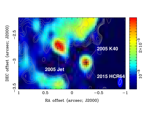
Figure 5: Images of the radio emission from the micro-quasar correspoding to the X-ray transient CXOGC J174540.0-290031, observed with the JVLA in the A-array at 33 GHz (contours) and 22.5 GHz (colors) on 2015-9-11 and 2005-9-16, respectively. At the bottom-right corner, the FWHM beams of 0.11”$\times$0.04” ($-11^{\rm o}$) and 0.2”$\times$0.1” (0^o) at 33 and 22.5 GHz are shown with a white and filled-blue ellipses. Contour values are $\sigma_{\rm im}\times$ (5.7, 8, 11.3, 16, 22.6 and 32), where $\sigma_{\rm im}=7\mu$Jy beam^-1. The two plus symbols mark the positions of K40 at 22.5 GHz in 2005 and of HCR22 at 33 GHz in 2015.

Table 2: A catalog of hypercompact radio sources at 44.6 and 33 GHz

ID	RA(J2000)	Dec(J2000)	$\left[S\pm\sigma\right]_{44.6}$	$\left[S\pm\sigma\right]_{33}$	$\theta_{maj}\pm\sigma$	$\theta_{min}\pm\sigma$	PA$\pm\sigma$	$\alpha_{44.6/33}\pm\sigma$	$\sigma_{\rm im}$, n1	Notes
	(   s   )	(   ”   )	(mJy)	(mJy)	(mas)	(mas)	(deg)		($\mu$Jy bm-1)
(1)	(2)	(3)	(4)	(5)	(6)	(7)	(8)	(9)	(10)	(11)
HCR01	40.6981(3)	18.323( 6)	$0.95\pm 0.11$	$1.00\pm 0.16$	$74.\pm 19.$	$56.\pm 17.$	$36.\pm 23.$	$-0.17\pm 0.65$	7.0,  6	ID925
HCR02	40.5194(4)	27.445( 7)	$0.20\pm 0.02$	$0.15\pm 0.02$	$68.\pm 11.$	$26.\pm 30.$	$30.\pm 45.$	$0.96\pm 0.60$	7.0,  5
HCR03	40.3836(1)	23.150( 3)	$0.27\pm 0.02$	$0.20\pm 0.02$	$57.\pm 14.$	$40.\pm 8.$	$150.\pm 36.$	$1.00\pm 0.48$	7.0,  5
HCR04	40.2641(1)	33.686( 3)	$0.26\pm 0.02$	$0.22\pm 0.01$	$45.\pm 13.$	$16.\pm 8.$	$100.\pm 13.$	$0.55\pm 0.38$	7.0,  7	IRS 9W21
HCR05	40.2679(1)	29.243( 3)	$0.22\pm 0.02$	$0.19\pm 0.02$	unresolved			$0.49\pm 0.52$	7.0,  8	ID425
HCR06	40.2629(1)	27.217( 1)	$0.80\pm 0.04$	$0.75\pm 0.04$	$20.\pm 6.$	$15.\pm 9.$	$80.\pm 42.$	$0.21\pm 0.25$	7.0,  5	ID225
HCR07	40.1708(1)	29.788( 1)	$2.54\pm 0.13$	$1.90\pm 0.10$	$20.\pm 8.$	$8.\pm 8.$	$56.\pm 47.$	$0.96\pm 0.24$	7.0,  9	Magnetar1
HCR08	40.1449(4)	16.419(13)	$0.23\pm 0.02$	$0.21\pm 0.02$	$19.\pm 10.$	$13.\pm 20.$	$80.\pm 24.$	$0.30\pm 0.32$	7.0,  6
HCR09	40.1286(1)	29.060( 4)	$0.21\pm 0.02$	$0.27\pm 0.02$	$49.\pm 23.$	$18.\pm 11.$	$84.\pm 30.$	$-0.83\pm 0.46$	7.0,  7	ID325
HCR10	40.1166(1)	27.526( 1)	$0.36\pm 0.03$	$0.33\pm 0.03$	$15.\pm 16.$	$4.\pm 17.$	$22.\pm 44.$	$0.29\pm 0.36$	7.0,  5	ID125
HCR11	40.1067(6)	22.277( 9)	$0.11\pm 0.02$	$0.17\pm 0.01$	$61.\pm 31.$	$26.\pm 9.$	$82.\pm 21.$	$-1.45\pm 0.68$	7.0,  5	IRS 7E2
HCR12	39.9905(6)	30.154(12)	$0.19\pm 0.01$	$0.33\pm 0.03$	$51.\pm 10.$	$44.\pm 6.$	$38.\pm 18.$	$-1.83\pm 0.42$	7.0,  7
HCR13	39.9683(6)	29.907(12)	$0.25\pm 0.03$	$0.40\pm 0.04$	$95.\pm 18.$	$34.\pm 6.$	$94.\pm 28.$	$-1.56\pm 0.57$	8.5,  7
HCR14	39.9502(1)	30.636( 3)	$0.31\pm 0.02$	$0.40\pm 0.04$	$74.\pm 10.$	$59.\pm 9.$	$158.\pm 64.$	$-0.85\pm 0.36$	7.0,  6
HCR15	39.9380(3)	31.162( 6)	$0.16\pm 0.02$	$0.29\pm 0.02$	$72.\pm 16.$	$18.\pm 33.$	$90.\pm 20.$	$-1.97\pm 0.53$	8.0,  6	Mini-cavity7
HCR16	39.9350(3)	31.370( 6)	$0.59\pm 0.07$	$0.82\pm 0.05$	$81.\pm 17.$	$62.\pm 18.$	$134.\pm 32.$	$-1.09\pm 0.43$	8.0,  6	Mini-cavity7
HCR17	39.9151(3)	28.563( 7)	$0.52\pm 0.07$	$0.69\pm 0.11$	$81.\pm 29.$	$60.\pm 21.$	$166.\pm 90$	$-0.94\pm 0.66$	7.0,  6	$\epsilon^{8}$
HCR18	39.9096(1)	30.895( 4)	$0.17\pm 0.02$	$0.31\pm 0.03$	$48.\pm 14.$	$29.\pm 20.$	$134.\pm 24.$	$-1.99\pm 0.50$	8.0,  6	Mini-cavity7
HCR19	39.9013(1)	30.053( 3)	$0.41\pm 0.03$	$0.54\pm 0.04$	$82.\pm 9.$	$60.\pm 11.$	$98.\pm 24.$	$-0.91\pm 0.34$	8.0,  6	Mini-cavity9, ID1825
HCR20	39.8952(6)	28.230(12)	$0.20\pm 0.03$	$0.38\pm 0.04$	$60.\pm 23.$	$56.\pm 23.$	$144.\pm 59.$	$-2.13\pm 0.61$	7.0,  6	$\epsilon^{8}$
HCR21	39.8883(3)	31.088( 7)	$0.32\pm 0.04$	$0.56\pm 0.03$	$87.\pm 20.$	$64.\pm 16.$	$158.\pm 77.$	$-1.86\pm 0.49$	8.0,  6
HCR22	39.8408(3)	19.316( 6)	$<0.06$	$0.15\pm 0.02$	$73.\pm 16.$	$50.\pm 61.$	$73.\pm 82.$	N/A	7.0,  6	PWN3
HCR23	39.8407(1)	29.442( 4)	$0.92\pm 0.08$	$1.00\pm 0.11$	$84.\pm 12.$	$44.\pm 30.$	$14.\pm 8.$	$-0.28\pm 0.46$	8.0,  7	Mini-cavity10, ID2025
HCR24	39.8345(1)	29.548( 3)	$0.19\pm 0.01$	$0.20\pm 0.01$	unresolved			$-0.17\pm 0.34$	8.0,  7	Mini-cavity10, ID1925
HCR25	39.8272(1)	29.810( 4)	$0.88\pm 0.08$	$1.29\pm 0.13$	$49.\pm 18.$	$34.\pm 19.$	$20.\pm 52.$	$-1.27\pm 0.45$	8.0,  7	IRS 13E-SE6, ID3225
HCR26	39.8247(1)	29.521( 3)	$0.29\pm 0.02$	$0.25\pm 0.02$	unresolved			$0.49\pm 0.42$	8.0,  7	IRS 13E-NE11, ID2125
HCR27	39.8236(3)	30.039( 7)	$0.21\pm 0.03$	$0.37\pm 0.04$	$45.\pm 22.$	$25.\pm 28.$	$133.\pm 52.$	$-1.88\pm 0.64$	8.0,  7	IRS 13E-SE6
HCR28	39.8235(3)	31.825( 6)	$0.35\pm 0.04$	$0.45\pm 0.03$	$73.\pm 16.$	$36.\pm 8.$	$20.\pm 16.$	$-0.83\pm 0.47$	7.0,  8	Mini-cavity12
HCR29	39.8210(1)	29.311( 4)	$0.30\pm 0.03$	$0.50\pm 0.03$	$44.\pm 12.$	$34.\pm 20.$	$148.\pm 36.$	$-1.70\pm 0.41$	8.0,  7	IRS 13E-NE11, ID2325
HCR30	39.8181(1)	29.475( 4)	$0.20\pm 0.02$	$0.28\pm 0.02$	$58.\pm 5.$	$22.\pm 2.$	$164.\pm 3.$	$-1.12\pm 0.47$	8.0,  7	IRS 13E-NE11, ID2225
HCR31	39.8180(1)	28.902( 6)	$0.63\pm 0.03$	$0.93\pm 0.06$	$87.\pm 5.$	$42.\pm 7.$	$98.\pm 7.$	$-1.29\pm 0.26$	8.0,  9	IRS 13E-NE13
HCR32	39.8165(2)	30.861( 7)	$<0.06$	$0.42\pm 0.03$	$40.\pm 5.$	$11.\pm 22.$	$72.\pm 4.$	N/A	7.0,  7	Mini-cavity14
HCR33	39.8121(1)	29.860( 3)	$0.35\pm 0.03$	$0.58\pm 0.05$	$48.\pm 14.$	$16.\pm 10.$	$14.\pm 22.$	$-1.68\pm 0.43$	8.0,  7	IRS 13E-SE6, ID3025
HCR34	39.8107(1)	31.739( 4)	$0.30\pm 0.03$	$0.45\pm 0.04$	$93.\pm 14.$	$45.\pm 6.$	$8.\pm 12.$	$-1.35\pm 0.46$	7.0,  6	Mini-cavity12
HCR35	39.8075(1)	29.300( 3)	$0.42\pm 0.03$	$0.43\pm 0.05$	$55.\pm 10.$	$22.\pm 26.$	$62.\pm 24.$	$-0.08\pm 0.42$	7.0,  8	IRS 13E-NE11, ID2425
HCR36	39.8007(3)	29.020( 6)	$0.31\pm 0.04$	$0.58\pm 0.04$	$42.\pm 8.$	$27.\pm 16.$	$56.\pm 27.$	$-2.08\pm 0.50$	8.0,  6	IRS 13E-N15, ID2825
HCR37	39.7967(6)	30.914( 9)	$0.18\pm 0.04$	$0.41\pm 0.03$	$72.\pm 25.$	$41.\pm 55.$	$36.\pm 44.$	$-2.73\pm 0.79$	8.0,  7	IRS 2-N16
HCR38	39.7961(1)	29.662( 3)	$5.50\pm 0.38$	$3.35\pm 0.42$	$78.\pm 18.$	$42.\pm 18.$	$52.\pm 21.$	$1.65\pm 0.47$	8.0,  12	IRS 13E5, ID3325
HCR39	39.7941(3)	29.844( 9)	$1.27\pm 0.12$	$1.14\pm 0.09$	$76.\pm 17.$	$29.\pm 5.$	$90.\pm 7.$	$0.36\pm 0.41$	8.0,  6	IRS 13E-S17, ID3425
HCR40	39.7895(1)	28.540( 4)	$0.58\pm 0.05$	$0.69\pm 0.04$	$94.\pm 9.$	$54.\pm 3.$	$91.\pm 5.$	$-0.58\pm 0.34$	8.0,  6	Triplet18
HCR41	39.7891(3)	29.508( 7)	$0.90\pm 0.12$	$1.10\pm 0.07$	$61.\pm 20.$	$41.\pm 30.$	$150.\pm 38.$	$-0.67\pm 0.49$	8.0,  7	IRS 13E-W19
HCR42	39.7857(3)	31.239( 6)	$0.67\pm 0.05$	$1.00\pm 0.06$	$84.\pm 11.$	$52.\pm 7.$	$166.\pm 12.$	$-1.33\pm 0.32$	8.0,  7	IRS 2
HCR43	39.7855(1)	28.421( 4)	$0.30\pm 0.03$	$0.48\pm 0.05$	$68.\pm 16.$	$46.\pm 11.$	$161.\pm 30.$	$-1.56\pm 0.49$	8.0,  6	Triplet18
HCR44	39.7799(1)	29.587( 4)	$1.23\pm 0.13$	$1.23\pm 0.10$	$46.\pm 18.$	$22.\pm 17.$	$36.\pm 33.$	$0.00\pm 0.45$	8.0,  7	IRS 13E-W19, ID3525
HCR45	39.7764(3)	31.938( 3)	$1.48\pm 0.09$	$1.15\pm 0.08$	$96.\pm 10.$	$40.\pm 4.$	$1.\pm 5.$	$0.84\pm 0.31$	8.0,  8	IRS 2L, ID3625
HCR46	39.7721(1)	29.678( 7)	$0.64\pm 0.06$	$0.68\pm 0.04$	$90.\pm 11.$	$56.\pm 14.$	$78.\pm 16.$	$-0.20\pm 0.36$	8.0,  7	IRS 13E-W19
HCR47	39.7721(2)	31.154( 9)	$0.18\pm 0.03$	$0.15\pm 0.03$	$44.\pm 18.$	$21.\pm 6.$	$82.\pm 10.$	$0.61\pm 0.90$	7.0,  5	IRS 2
HCR48	39.7699(1)	29.479( 7)	$0.10\pm 0.02$	$0.19\pm 0.01$	$35.\pm 24.$	$16.\pm 14.$	$59.\pm 34.$	$-2.13\pm 0.73$	8.0,  7	IRS 13E-W19
HCR49	39.7697(3)	25.913( 7)	$0.17\pm 0.02$	$0.21\pm 0.04$	$65.\pm 19.$	$39.\pm 13.$	$78.\pm 14.$	$-0.70\pm 0.78$	7.0,  7	Bullet SE4
…	39.7671(4)	25.909( 6)	$0.13\pm 0.02$	$0.16\pm 0.04$	$63.\pm 14.$	$23.\pm 05.$	$5.\pm 10.$	$-0.69\pm 1.00$	…	Bullet NW4
HCR50	39.7677(1)	29.824( 3)	$0.27\pm 0.02$	$0.30\pm 0.03$	$47.\pm 13.$	$28.\pm 14.$	$72.\pm 31.$	$-0.35\pm 0.42$	8.0,  7	IRS 13E-W19
HCR51	39.7672(1)	31.378( 3)	$0.19\pm 0.01$	$0.24\pm 0.02$	unresolved			$-0.78\pm 0.40$	7.0,  7	IRS 2-W
HCR52	39.7620(4)	29.783( 4)	$0.31\pm 0.04$	$0.47\pm 0.03$	$24.\pm 1.$	$16.\pm 1.$	$60.\pm 3.$	$-1.38\pm 0.49$	8.0,  7	IRS 13E-W19
HCR53	39.7513(1)	30.675( 3)	$0.36\pm 0.02$	$0.30\pm 0.03$	$80.\pm 11.$	$14.\pm 41.$	$20.\pm 3.$	$0.61\pm 0.34$	7.0,  9	IRS 13E-SW20
HCR54	39.7461(3)	26.567(10)	$0.11\pm 0.02$	$0.15\pm 0.02$	$28.\pm 10.$	$12.\pm 21.$	$60.\pm 10.$	$-1.03\pm 0.78$	7.0,  8	IRS 34SW22
HCR55	39.7439(4)	31.215( 6)	$0.57\pm 0.08$	$0.86\pm 0.14$	$81.\pm 22.$	$53.\pm 46.$	$108.\pm 98.$	$-1.37\pm 0.69$	7.0,  7
HCR56	39.7320(1)	30.580( 4)	$0.19\pm 0.02$	$0.36\pm 0.02$	$58.\pm 7.$	$38.\pm 6.$	$55.\pm 10.$	$-2.12\pm 0.43$	7.0,  8
HCR57	39.7299(1)	26.595( 3)	$0.33\pm 0.03$	$0.35\pm 0.03$	$38.\pm 17.$	$18.\pm 26.$	$60.\pm 42.$	$-0.20\pm 0.48$	7.0,  8	IRS 34SW22, ID625
HCR58	39.6399(1)	26.651( 4)	$0.19\pm 0.02$	$0.20\pm 0.02$	$76.\pm 18.$	$44.\pm 46.$	$124.\pm 53.$	$-0.17\pm 0.54$	7.0,  8	IRS 6E23
HCR59	39.6255(3)	26.623( 4)	$1.21\pm 0.08$	$1.40\pm 0.17$	$94.\pm 22.$	$68.\pm 7.$	$132.\pm 35.$	$-0.48\pm 0.47$	8.0,  8	IRS 6E23, ID3725
HCR60	39.5463(1)	35.005( 1)	$0.60\pm 0.04$	$0.50\pm 0.03$	$31.\pm 12.$	$16.\pm 50.$	$90.\pm 23.$	$0.61\pm 0.30$	7.0,  8	ID725
HCR61	39.4593(1)	31.736( 4)	$0.34\pm 0.03$	$0.31\pm 0.03$	unresolved			$0.31\pm 0.43$	7.0,  9	ID825
HCR62	39.3096(1)	30.683( 1)	$0.22\pm 0.01$	$0.18\pm 0.01$	$30.\pm 5.$	$9.\pm 2.$	$10.\pm 2.$	$0.67\pm 0.33$	7.0,  8
HCR63	39.2771(4)	27.332(12)	$0.22\pm 0.04$	$0.27\pm 0.02$	$51.\pm 33.$	$36.\pm 34.$	$42.\pm 48.$	$-0.68\pm 0.69$	7.0,  8
HCR64	40.0201(9)	31.178(20)	$<0.15$	$0.60\pm 0.07$	$140.\pm 20.$	$70.\pm 10.$	$134.\pm 10.$	N/A	8.0,  5	micro-qso,K4024

1The radio counterpart of SGR J1745-2900 (Eatough et al., 2013), the GC magnetar, and see Sec.4.3 of this paper. 2Located east of the IRS 7 bow-shock feature (Yusef-Zadeh & Morris, 1991). 3A candidate cannonball of the PWN G359.95-0.04 (Wang et al., 2006), and see Sec.4.1 of this paper. 4The head of the bullet (Zhao et al., 2009), resolved into two components. 5The radio core associated with IRS 13E. 6Located $\sim$0.5” SE of IRS 13E core (e.g., Tsuboi et al., 2017). 7Located within the mini-cavity. 8The $\epsilon$ source that has been resolved into three components (Yusef-Zadeh et al., 1990; Zhao et al., 1991), S (HCR17), NE and NW (HCR20); the three components correspond to RS6, RS5 and RS7 detected at 34.5 GHz (Yusef-Zadeh et al., 2016). 9Located in the northern mini-cavity. 10Located at the northwestern rim of the mini-cavity. 11Located 0.5” NE of the IRS 13E radio core. 12Located at the southwestern rim of the mini-cavity. 13Located 1” NE of the IRS 13E radio core. 14Located at the western rim of the mini-cavity. 15Located 0.7” N of the IRS 13E radio core. 16Located N of the IRS 2. 17Located 0.2” S of the IRS 13E radio core. 18A triplet located 1.2” N of the IRS 13E radio core, consisting of three components S(HCR40), NW(HCR43) and NE with a size larger than the HCR upper limit. 19Located 0.3” W of the IRS 13E radio core, the HCR41 group consisting of six members of HCR41, 44, 46, 48, 50 and 52. 20Located 1” SW of the IRS 13E radio core. 21Located in the IRS 9W region. 22Located in the IRS 34SW region. 23Located in the IRS 6E region. 24Located in the bar, a radio counterpart of the X-ray transients CXOGC J174540.029003 (Muno et al., 2005; Bower et al., 2005; Zhao et al., 2009) and see Sec.4.2 of this paper. 25The 7mm-sources are identified with IR stars emitting at 3.8 $\mu$m, among which HCR05 (ID4), HCR06 (ID2), HCR10 (ID1), HCR57 (ID6), HCR60 (ID7) and HCR61 (ID8) are associated with strong stellar winds (Yusef-Zadeh et al., 2014).

4.3 The GC magnetar: SGR J1745-2900

HCR07 is one of the most recognizable HCR members, as it is associated with the GC magnetar and has a high-energy counterpart, SGR J1745-2900. The soft gamma-ray repeater was discovered by Swift during a large X-ray outburst on 2013 April 24 (MJD 56406), powered by a magnetar close to Sgr A*(Kennea et al., 2013). The magnetar hypothesis was further supported by NuSTAR detections of periodic pulsed signal at 3.76 s (Mori et al., 2013). With the observations by Chandra and Swift, Rea et al. (2013) pinpointed the location of the magnetar at a projected distance of 2.4$\pm$0.3 arcsec from Sgr A*; and the authors also determined the source spin period and its derivative with high precision ($P=$3.7635537(2) s and $\dot{P}=6.61(4)\times 10^{-12}$ s s^-1). The magnetar, SGR J1745-2900, was monitored by the Chandra X-ray observatory for six years following the X-ray outburst in 2013 April, showing the long-term properties of the outburst (Rea et al., 2020).

Radio pulses from SGR J1745-2900 were first detected by the Effelsberg radio telescope and confirmed with other telescopes, including the Nancay telescope, JVLA, Jodrell Bank Observatory (Eatough et al., 2013), and the Australia Telescope Compact Array (ATCA) (Shannon & Johnston, 2013) at various frequencies between 1.5 and 19 GHz. High-frequency pulses were detected at 87, 101, 138, 154, 209 and 225 GHz with the IRAM-30m telescope during the period between 2014-7-21 (MJD 56859) and 2014-7-24 (MJD 56862) (Torne et al., 2015). In their follow-up campaign, Torne et al. (2017) detected high-frequency pulses with the IRAM-30m up to 291 GHz in the interval between 2015-3-4 (MJD 57085) and 2015-3-9 (MJD 57090). The high-frequency pulses were also detected at 45 GHz with the Green Bank Telescope (GBT) on 2014-4-10 (MJD 56757) (Gelfand et al., 2017).

4.3.1 A collection of flux-densitiy measurements from JVLA and ALMA

In addition to the JVLA and ALMA flux densities determined from the images reported in this work, we also collected the data from the prior published literature. Table 3 assembles all the available data from JVLA and ALMA observations at radio wavelengths. The table is configured into two main column sections, each of which consists of six sub-columns: (1) observing date; (2) the corresponding modified Julian day (MJD); (3) band center frequency in units of GHz; (4) flux densities in units of mJy and (5) the corresponding 1$\sigma$ uncertainties. For the non-detections, a 3$\sigma$ value is given for the upper limits. Finally, alphabetical codes are designated for the relevant references that are listed at the bottom notes of the table. The measurements reported for the first time in this paper are highlighted with a bold font.

Table 3: JVLA & ALMA flux densities of SGR J1745-2900

Obs. date	MJD	$\nu_{0}$ (GHz)	Sν (mJy)	$\sigma$ (mJy)	Ref.		Obs. date	MJD	$\nu_{0}$ (GHz)	Sν (mJy)	$\sigma$ (mJy)	Ref.
(1)	(2)	(3)	(4)	(5)	(6)		(1)	(2)	(3)	(4)	(5)	(6)
2011-08-04	55776	42	$<0.24^{\dagger}$	…	a		2012-10-14	56214	21.2	$<0.60^{\dagger}$	…	a
2012-10-14	56214	32	$<0.81^{\dagger}$	…	a		2012-10-14	56214	41	$<0.78^{\dagger}$	…	a
2012-12-22	56283	21.2	$<0.90^{\dagger}$	…	a		2012-12-22	56283	32	$<0.94^{\dagger}$	…	a
2012-12-22	56283	41	$<0.69^{\dagger}$	…	a		2013-05-10	56422	9	0.56	0.011	g
2013-06-01	56444	9	0.76	0.015	g		2013-06-30	56473	15	0.58	0.012	g
2013-07-13	56486	9	1 .47	0.030	g		2013-10-26	56591	21.2	$<1.95^{\dagger}$	…	a
2013-10-26	56591	32	$<1.45^{\dagger}$	…	a		2013-10-26	56591	41	$<0.82^{\dagger}$	…	a
2013-10-26	56591	41	0.7	0.4	e		2013-11-29	56626	21.2	$<2.04^{\dagger}$	…	a
2013-11-29	56626	32	$<0.82^{\dagger}$	…	a		2013-11-29	56626	41	$<0.70^{\dagger}$	…	a
2013-11-29	56626	41	0.89	0.08	e		2013-12-29	56656	21.2	$<1.70^{\dagger}$	…	a
2013-12-29	56656	32	$<0.86^{\dagger}$	…	a		2013-12-29	56656	41	$<1.52^{\dagger}$	…	a
2013-12-29	56656	41	1.20	0.7	e		2014-01-01	56658	15	2.09	0.042	g
2014-01-01	56658	9	1.18	0.024	g		2014-02-15	56703	21.2	0.84	0.33	a
2014-02-15	56703	32	1.83	0.10	a		2014-02-15	56703	41	1.85	0.07	a
2014-02-15	56703	41	2.1	0.4	e		2014-02-21	56709	44.6	1.62	0.04	a
2014-02-22	56710	15	1.07	0.022	g		2014-02-22	56710	9	0.94	0.019	g
2014-03-09	56731	34.5	1.30	0.01	a		2014-03-22	56738	21.2	2.79	0.19	a
2014-03-22	56738	32	2.64	0.05	a		2014-03-22	56738	41	1.24	0.02	a
2014-03-22	56738	41	2.1	0.3	e		2014-04-03	56750	23	0.92	0.019	g
2014-04-03	56750	43	0.54	0.011	g		2014-04-25	56772	9	1.00	0.020	g
2014-04-25	56772	15	1.22	0.025	g		2014-04-26	56743	21.2	0.90	0.14	a
2014-04-26	56743	32	0.62	0.04	a		2014-04-26	56743	41	1.20	0.07	a
2014-04-26	56743	41	0.91	0.30	e		2014-04-17	56764	9.0	3.50	0.08	b
2014-05-10	56787	41	1.15	0.05	e		2014-05-17	56794	5.5	4.50	0.24	b
2014-05-26	56803	5.5	3.90	0.09	b		2014-05-31	56808	21.2	4.21	0.17	a
2014-05-31	56808	32	2.90	0.13	a		2014-05-31	56808	41	2.94	0.12	a
2014-05-31	56808	41	3.5	0.4	e		2014-08-23	56892	15	0.63	0.013	g
2014-08-30	56899	23	0.26	0.006	g		2014-08-30	56899	43	0.15	0.003	g
2015-02-20	57073	9.0	3.00	0.30	b		2015-09-11	57276	33.0	1.80	0.05	b
2015-09-16	57281	44.6	2.45	0.05	b		2016-04-23	57502	343	2.80	0.23	b, d
2016-07-12	57581	44.2	5.79	0.05	f		2016-07-15	57584	226	4.70	1.29	f
2016-08-30	57630	343	3.10	0.11	b, d		2016-08-31	57631	343	3.29	0.12	b, d
2016-09-08	57639	343	3.90	0.13	b, d		2017-10-06	58032	225	1.41	0.08	b, c
2017-10-07	58033	225	1.53	0.08	b, c		2017-10-09	58035	225	0.79	0.07	b, c
2017-10-10	58036	225	1.22	0.06	b, c		2017-10-11	58037	225	1.25	0.07	b, c
2017-10-12	58038	225	1.44	0.07	b, c		2017-10-14	58040	225	3.16	0.08	b, c
2017-10-17	58043	225	5.34	0.09	b, c		2017-10-18	58044	225	5.42	0.11	b, c
2017-10-20	58046	225	5.60	0.12	b, c		2019-09-08	58734	5.5	$<0.50^{\dagger}$	…	b
2019-09-21	58747	9.0	0.40	0.10	b		2019-09-20	58748	318	1.32	0.15	b
2020-11-27	59180	9.0	0.36	0.06	b

†A 3-$\sigma$ upper limit. Reference: a. Yusef-Zadeh et al. (2015). b. This paper. c. The ALMA observations at the ten epochs were carried out by the PI Tsuboi in (Tsuboi et al., 2017). We re-processed the ALMA archival data (2017.1.00500.S) and determined the flux densities of SGR J1745-2900 at 225.75 GHz. d. Detected in the ALMA image made from observations on 2016-4-23, 2016-8-30/31, and 2016-9-8 (Tsuboi et al., 2017). We re-processed the ALMA archival data (2015.1.01080.S) and determined the flux densities of SGR J1745-2900 from each of the 340-GHz images at the four epochs. e. Mean values determined from two VLA Q-band measurements with a baseline filter ($>500$ k$\lambda$) and all data (Gelfand et al., 2017); for the case of std = 0, the smaller error in the two measurements is adopted. f. Yusef-Zadeh et al. (2017). g. Bower et al. (2015/16).

Figure 6: Averaged spectrum of SGR J1745-2900, made with band-averaged flux densities observed with the JVLA and ALMA (values summarized in Table 3) as well as with ATCA (Shannon & Johnston, 2013).

4.3.2 Radio spectrum of the GC magnetar

In addition to the JVLA and ALMA data, we also collected the flux-density data of the magnetar from ATCA (Shannon & Johnston, 2013), yielding a total of 91 flux-density measurements of this object at radio wavelengths over the 6.5 yrs since the 2013 outburst. To investigate the spectrum of the magnetar, we binned the data into nine bands with frequency ranges corresponding to those used for the ALMA and JVLA observing bands. We then computed the mean flux density ($\overline{\rm S}_{\nu}$) and variance ($\sigma_{\nu}^{2}$) in each of the bands, weighted by $wt(i)=\sigma(i)^{-2}$ where $\sigma(i)$ is the uncertainty of each individual flux density, $i$. For non-detections, a zero weight was adopted, assuming that the actual uncertainties of the non-detections due to the errors in the calibration for the system and atmostheric issues are much greater than the cited rms errors. For a total of $n$ measurements in each bin, the number of non-zero weighted data points, $m$, is less than or equal to $n$, (${m\leq n}$), within each bin. The error of the mean flux density can be determined with

$$\sigma_{\overline{\rm S}_{\nu}}=\sqrt{\sigma_{\nu}^{2}\over{m}}.$$

We note that the Ka band shows a lower detection rate ($\sim$55%) than the Q-band ($\sim$68%), indicating that a spectral minimum is located near the Ka-band frequency of 33 GHz, given the fact that the rms noise at the Ka-band center frequency of 33 GHz is about a factor of 2 smaller than that of Q-band (see Table 1). To reduce the bias due to zero-weighting on the data with negative detections, we combined the Ka-band and Q-band bins’ data and re-computed the mean flux density and its uncertainty. Table 4 summarizes the results. Fig. 6 shows the averaged spectra observed with the JVLA, ALMA and ATCA over 6.5 yrs since the outburst. The vertical bars on each point reflect the large intrinsic variation of the flux density from SGR J1745-2900 over the observed time scale. However, a spectral minimum appears to be present at a frequency around 30 GHz, hereafter referred to as the transition frequency $\nu_{\rm t}$, which appears to separate the spectrum into two components arising from two emission regimes at centimeter and millimeter-submillimeter wavelengths. The flux density of the centimeter-wave component is typically $\sim$1 mJy while the millimeter-wave component is about three times more intense.

Table 4: Mean flux densities of SGR J1745-2900 in the JVLA/ALMA bands

Band code	$n$	$m$	$\overline{\nu}\pm\Delta\nu$ (GHz)	$\overline{\rm S}_{\nu}\pm\sigma_{\overline{\rm S}_{\nu}}$ (mJy)
(1)	(2)	(3)	(4)	(5)
A7	5	5	338.0$\pm$5.0	3.01$\pm$0.41
A6	11	11	225.1$\pm$ 0.1	2.14$\pm$0.51
Q-Ka	34	23	39.4$\pm$ 0.9	0.33$\pm$0.10
K	15	10	20.7$\pm$ 0.5	0.30$\pm$0.07
Ku	7	7	15.3$\pm$ 0.2	0.69$\pm$0.13
X	12	12	8.9$\pm$ 0.1	0.82$\pm$0.10
C	7	6	5.5$\pm$ 0.4	1.16$\pm$0.37

The band-averaged data are derived from the individual flux-density measurements with the JVLA and ALMA (Table 3) as well as ATCA (Shannon & Johnston, 2013).

We then carried out a least-squares fitting of the spectrum to both the cm- and mm-components with two power-law functions. The centimeter data are well fit with a power-law spectral index of $\alpha_{\rm cm}=-1.5\pm 0.6$ ($S_{\nu}\propto\nu^{\alpha_{\rm cm}}$), a steep spectrum similar to that of radio pulsars. A steep spectrum of $\alpha=-1$ was previously reported between 4.5 and 8.5 GHz for the observations during the 2013-5-30 flare of the cm-component (Shannon & Johnston, 2013). The spectral data points rising through millimeter wavelengths can be fit with a spectral index of $\alpha_{\rm mm}=1.1\pm 0.2$, indicating the presence of an emission bump or a plateau at higher frequencies. Such a high-frequency plateau appears not to be unique to the GC magnetar. The radio-active magnetar 1E 1547.0$-$5408 has also been observed to have a spectrum rising towards millimeter wavelengths (Chu et al., 2021). Overall, the spectrum of the GC magnetar at the frequencies in the range between 5 and 310 GHz is described with a combination of the two power-law functions (see Fig. 6) with a transition frequency $\nu_{\rm t}\approx 30$ GHz corresponding to a minimum flux density of $\sim$0.3 mJy.

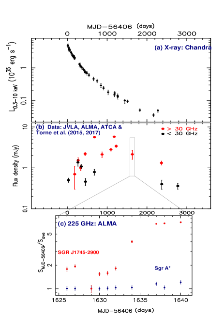
Figure 7: (a) The X-ray luminosity variation after the onset of outburst of SGR J1745-2900, observations by the Chandra X-ray observatory (Rea et al., 2020). (b) 100-MJD bin averaged radio light curve of the magnetar J1745-2900 for both the mm- (red dots) and cm- (black dots) components. In addition to the flux-density measurements from the JVLA and ALMA summarized in Table 3, other telescope data from literatures (Shannon & Johnston, 2013; Torne et al., 2015, 2017) are included. (c) Detail of ALMA observations in the interval between 2017-10-6 and 2017-10-20 (1626 days after the outburst of SGR 1745-2900 on 2013-4-23) show a day-to-day variability of the magnetar SGR J1745-2900 at 225 GHz displayed as normalized flux densities S_MJD-56406/S_min (red dots), where the minimum flux density S${}_{min}=$0.79$\pm$0.08 mJy for the magnetar on MJD 58035. The variability of SGR J1745-2900 during the two-week interval is compared with that of Sgr A* (dark-blue dots); Sgr A* (S_min=3.015$\pm$0.013 Jy and S_ave= 3.26$\pm$0.09 Jy) that is three orders in magnitude more luminous than the magnetar.

4.3.3 Radio variability of SGR J1745-2900

We inspected the radio variability of the GC magnetar SGR J1745-2900, including a total of 161 flux-density measurements since the onset of the 2013 outburst. The measurements by Torne et al. (2015, 2017) are also included in addition to the JVLA-ALMA (Table 3) and ATCA (Shannon & Johnston, 2013) data. The magnetar appears to be highly variable on all observed time scales and wavelengths (e.g. Shannon & Johnston, 2013; Yusef-Zadeh et al., 2015, and this paper). We utilized a bin-averaging algorithm similar to the analysis of the magnetar spectrum (Sec.4.3.2). We binned the MJD or the time axis with a constant interval of 100 days. The two spectral components $--$ low-frequency and high-frequency $--$ corresponding to the cm-component ($\nu<30$ GHz) and the mm-component ($\nu>30$ GHz), were examined separately. We then computed the weighted mean flux densities and the corresponding dispersions in each of the 56 MJD-bins for both mm- and cm-components. The results for the non-empty bins are tabulated in Table 5. Columns 1 and 2 show the bin ID (binID) and the corresponding central MJD. Columns 3 and 4 are the numbers of all the measurements ($n$) and the non-zero weight data ($m$) in the corresponding MJD-bins; as above, the measurements with only upper limits are zero-weighted. Column 5 is the mean MJD of the observing dates. Column 6 gives the mean flux-density ($\overline{S}_{\rm binID}$), weighted by the inverse variance on each of the measurements, along with the uncertainty of the mean $\sigma_{\overline{S}_{\rm binID}}=\sqrt{\sigma^{2}_{\rm binID}/{m}}$. And the standard deviation ($\sigma_{\rm binID}$), or the dispersion due mainly to the variation in flux density, is listed in column 7.

Fig. 7b plots the MJD-bin averaged radio light curves for the two spectral components, red for mm and black for cm. Unlike the X-ray light curve (Fig. 7a) observed by the Chandra X-ray observatory (Rea et al., 2020) that shows a smooth decrease in X-ray luminosity, both the cm- and mm-components varied significantly in the first 800 and 1700 days. Our two measurements of flux density based on the earlier JVLA observations at 5.5 GHz showed a significant variation from 4.50$\pm$0.24 mJy on 2014-05-17 to 3.90$\pm$0.09 mJy on 2014-05-26, on the time scale of a week, which is consistent with the large variability at 5 GHz observed during May 2013 (Shannon & Johnston, 2013).

The two most recent JVLA measurements at 9 GHz on 2020-11-27 (MJD 59180) and 2019-09-21 (MJD 58777) indicate that the flux density of the cm-component decreased to 0.4 mJy from 3.5 mJy in the JVLA observation on 2014-04-17 (MJD 56764). Also, we failed to detect the source at 5.5 GHz based on the JVLA observations on 2019-09-08 (58734), imposing a 3-$\sigma$ upper limit of 0.5 mJy while the flux density was 4.5 mJy based on our JVLA observation at 5.5 GHz on 2014-5-17 (MJD 56794). The mean flux density of the cm-component of the magnetar decreased by a factor of 3 over a period of 6.5 yr (Fig. 7b and Table 5).

The Chandra X-ray observations of SGR J1745-2900 following the outburst show a smooth decrease from 4.9$\times 10^{35}$ erg ^-1 at the onset of the X-ray outburst to 0.047$\times 10^{35}$ erg ^-1 at the most recent epoch (Fig. 7a). The X-ray luminosity therefore dropped by two orders in magnitude over 6 years. The general trend of decreasing radio flux density is consistent with the X-ray light curve, although the cm-component has a much slower decline, is much more variable, and shows a large range of variability on time scales from days to years.

The mm-component stayed at a relatively low level, with bin-averaged flux densities of 0.7$\pm$0.40 and 1.53$\pm$0.23 mJy during the second and third MJD-bins after the outburst (Table 5 and Fig. 7b). During the first 300 days, the mm-component was difficult to detect (only 5 detections out of 11 observations). We note that the JVLA Q-band data observed during 2013 fall and 2014 spring were reduced by two independent groups (Yusef-Zadeh et al., 2015; Gelfand et al., 2017). The mm-component reached a maximum of 5.63$\pm$0.19 mJy in the 7th MJD-bin (601-700 days after the outburst), based on 35 observations with a detection rate of 100%.

The 17th MJD bin of the mm-component (between 1600-1700 days) contains 10 individual ALMA observations at 225 GHz, all carried out within a two-week period during October 2017 with a high-resolution (0.02”) configuration (Tsuboi et al., 2019). The mean flux density for the mm-component in this bin was 2.25$\pm$0.56 mJy. With this configuration, the extended HII emission, as well as dust emission from the local medium, are well resolved out and only hyper-compact sources can be detected. The typical rms noise of the ALMA images is about 20-30 $\mu$Jy beam^-1, and the magnetar has S/N ratios of 50-100. At a distance of $\sim$3” from the magnetar, Sgr A*, with a flux density near 3 Jy, is an excellent reference source to examine the day-to-day variability of the magnetar. The ALMA data show the magnetar to be highly variable at 225 GHz on a time scale of days. The source started at 1.41$\pm$0.08 mJy on 2017-10-6, dropped to a minimum of 0.79$\pm$0.08 mJy three days later on 2017-10-9, and then increased by a factor 7 within 8 days reaching 5.34$\pm$0.09 mJy on 2017-10-17, staying at that level for the next several days. To compare the variability of SGR J1745-2900 with Sgr A*, we normalized the source flux densities by their own minimum flux densities during the observing period. Fig. 7c shows the relative variability for both the magnetar and Sgr A* during the two weeks in bin 17. We define a relative variability parameter, $\mathscr{RV}$, to quantitatively describe the magnitude of variability relative to a minimum flux density $S_{\rm min}$, given a maximum flux density $S_{\rm max}$ of a target source observed in a period:

$$\mathscr{RV}={\left[{\rm S_{\rm max}-S_{\rm min}}\right]\over{\rm S_{\rm min}}}.$$

The magnetar shows the relative variability $\mathscr{RV}\approx$ 6 while Sgr A* is observed to be only moderately variable in the same ALMA program, with $\mathscr{RV}\approx$ 0.2..

Finally, the latest available detections of the magnetar in 2019-2020, are 1.32$\pm$0.15 mJy at 318 GHz with ALMA on 2019-09-20 (MJD 58748) and 0.36$\pm 0.06$ mJy with the JVLA on 2020-11-27 (MJD 59180).

Table 5: Mean flux densities of SGR J1745-2900 in 100-day MJD bins

binID	MJD	$n$	$m$	$\overline{\rm MJD}$	$\overline{\rm S}_{\rm binID}\pm\sigma_{\overline{\rm S}_{\rm binID}}$	$\sigma_{\rm binID}$
	(day)			(day)	(mJy)	(mJy)
(1)	(2)	(3)	(4)	(5)	(6)	(7)
Centimeter-wave component
1	56456	16	16	56435.1	0.50$\pm$0.06	0.24
3	56656	5	3	56673.2	1.36$\pm$0.26	0.45
4	56756	10	10	56755.7	1.08$\pm$0.14	0.44
5	56856	12	12	56862.4	0.46$\pm$0.09	0.31
7	57056	10	10	57085.9	0.79$\pm$0.13	0.41
24	58756	2	1	58777.0	0.40$\pm$0.10	0.10
28	59156	1	1	59180.0	0.36$\pm$0.06	0.06
Millimeter-wave component
2	56556	3	1	56591.5	0.70$\pm$0.40	0.40
3	56656	9	5	56678.6	1.53$\pm$0.23	0.51
4	56756	10	10	56742.4	1.00$\pm$0.14	0.44
5	56856	26	21	56853.2	2.20$\pm$0.21	0.96
7	57056	37	37	57087.3	5.63$\pm$0.19	1.16
9	57256	2	2	57278.5	2.13$\pm$0.32	0.45
11	57456	1	1	57502.0	2.80$\pm$0.23	0.23
12	57556	2	2	57582.5	5.78$\pm$0.04	0.06
13	57656	3	3	57633.3	3.40$\pm$0.23	0.40
17	58056	10	10	58038.4	2.14$\pm$0.53	1.68
24	58756	1	1	58770.0	1.32$\pm$0.15	0.15

The 100-day-averaged data are derived from a total of 161 individual flux-density measurements with the JVLA, ALMA (Table 3), ATCA (Shannon & Johnston, 2013) and other single-dish telescopes (Torne et al., 2015, 2017) since the onset of the outburst at the epoch 2013-4-23 (MJD 56406).

5 Astrophysical implications

A population of hyper-compact radio sources (HCRs) are detected at 33 and 44.6 GHz with the JVLA in the vicinity of Sgr A* within a radius of 13 arcsec. The new survey was motivated by the previous JVLA detections of 110 Galactic center compact radio sources (GCCRs) at 5.5 GHz in the radio bright zone within a radius of 7.5 arcmin from Sgr A* but outside Sgr A West.

5.1 Spectral types of HCRs & their distribution in flux-density

Fig. 8 shows the flux-density distribution of the HCRs as compared with that of the GCCRs. The distribution of the GCCRs is similar to the high-luminosity tail of the pulsars’ distribution in the Galactic disk (Kramer et al., 1998; Manchester et al., 2005; Zhao, Morris & Goss, 2020). The HCRs have a relatively narrow distribution from $-1$ to 0.6 in Log(S [mJy]), or ranging from 0.1 to 4 mJy, peaked at $-0.4$ in Log(S [mJy]) or 0.4 mJy. We note that the flux density of the peak in the HCR distribution is close to the minimum value 0.32 mJy at the transition frequency observed in the band-averaged spectrum for the GC magnetar J1745-2900 (see Sec.4.3.2).

We divided the HCRs into three sub-types according to their spectral indices $\alpha_{44.6/33}$ ($S\propto\nu^{\alpha_{44.6/33}}$) derived between 44.6 and 33 GHz: flat ($0.2\geq\alpha_{44.6/33}>-0.5$), steep ($\alpha_{44.6/33}\leq-0.5$) and inverted ($\alpha_{44.6/33}>0.2$).

Of all the HCRs, 58% (38/65) are steep-spectrum sources, 26% (17/65) are inverted-spectrum sources, and 15% (10/65) have a flat spectrum. We note that HCR49 is a double; so a total of 65 HCR components are included in the spectral-index analysis. The inset of Fig. 8 shows the flux-density distributions for each of the three spectral types with a finer bin, $\Delta$Log(S [mJy]) = 0.2.

5.1.1 Flat-spectrum HCRs

The flux density distribution of the flat-spectrum HCRs appears to be uniform within the range from 0.16 to 1.6 mJy. Some fraction of the flat-spectrum HCRs might be unresolved peaks in the HII region components since a flat spectrum at Ka- and Q-bands is characteristic of free-free emission in optically thin HII regions.

5.1.2 Steep-spectrum HCRs

This sub-sample consists of 38 members, the largest sub-sample among the three, in which the flux densities are statistically well distributed. The distribution can be fitted with a Gaussian, with a mean value of $\mu=-0.35$ and a standard deviation of $\sigma=0.22$ in Log(S [mJy]). The mean value of the steep-spectrum HCRs corresponds to 0.45 mJy in flux density.

The spectral index $\alpha_{44.6/33}$ of the steep-spectrum HCRs is in the range between $-6.5$ and $-0.6$, giving a mean $\mu_{\alpha}=-1.8\pm 0.2$. The steep spectrum of this sub-sample differs distinctly from the HII components, suggesting the presence of a population of hyper-compact nonthermal radio sources in the central parsec. The nonthermal HCRs are likely associated with the massive stellar remnants that are expected to be distributed in the close vicinity of Sgr A* (Morris, 1993; Hailey et al., 2018; Generozov et al., 2018).

5.1.3 Inverted-spectrum HCRs

For this sub-sample, the mean flux density and standard deviation are $\mu=0.5$ mJy and $\sigma=0.25$ mJy, respectively. The spectral index $\alpha_{44.6/33}$ of the inverted-spectrum HCRs is in the range between 0.21 and 1.65, with a mean value of $\mu_{\alpha}=0.61\pm 0.08$. Among the three spectral sub-samples, the distribution of the inverted-spectrum HCRs appears to most closely follow the GCCR distribution, which matches the high-luminosity tail of the distribution that normal pulsars would have at the Galactic center (Zhao, Morris & Goss, 2020). Normal pulsars usually have a steep spectrum at centimeter wavelengths and are difficult to detect at high frequencies. However, the GC magnetar, emitting at the Ka- and Q-bands, falls into this sub-sample. As shown in Sec. 4.3.2, an inverted spectral component of SGR J1745-2900 is present at millimeter wavelengths in the averaged spectrum of a large sample of observations. The inverted spectrum cannot be simply attributed to time variability of the flux density. By analogy with SGR J1745-2900, the inverted spectral component could be indicative of an association of the HCRs with magnetars.

On the other hand, hyper-compact HII regions associated with a late-type massive star may also have a similar characteristics in spectral index, flux density level and compactness. For example, a group of compact components have been detected at mm-submm wavelengths in the IRS 21 complex (see Fig. 2b). The hyper-compact sources associated with IR emission more likely belong to hyper-compact HII or HC HII regions associated with young stellar objects rather than old massive stellar remnants. The hyper-compact radio components of IRS 21 are therefore not included in the HCR catalog (Table 2) in this paper. IRS 21 will be discussed in a separate paper.

From cross-correlation between the HCRs of this paper and the nine 7mm-IR sources that are found to be associated with strong stellar winds (Yusef-Zadeh et al., 2014), we find that six of the nine candidate IR stars have HCR counterparts. The spectral indices of the six HCRs – five with inverted spectra and one with a flat spectrum – are consistent with the radio emission produced by the ionized winds of hot, massive stars (Panagia & Felli, 1975). Thus, a large fraction of the 17 inverted-spectrum HCRs might consist of thermal free-free emission sources. Apparently, a significant portion of the inverted-spectrum HCRs is associated with late-type massive stars.

We speculate that more magnetars besides SGR J1745-2900 reside in our inverted-spectrum sample of HCRs. However, we must be able to distinguish such objects from compact radio sources associated with young massive stars. Further high-resolution ALMA observations of the variability and polarization characteristics of this subsample will be crucial for identifying the nonthermal nature of candidate magnetars and stellar-mass black holes.

Figure 8: Flux-density distribution of the HCRs at 33 GHz within the central 13”$\times$13” region versus the GCCRs (Zhao, Morris & Goss, 2020) detected in the GC radio bright zone (15’$\times$15’). The grey histogram represents the 110 GCCRs detected at 5.5 GHz outside Sgr A West. The 64 HCRs (65 components, HCR49 is double), shown by the hatched histograms, are divided into three types: flat $-0.5<\alpha\leq 0.2$ (red), steep $\alpha\leq-0.5$ (green) and inverted $\alpha\geq 0.2$ (blue), according to their radio spectral index determined between 44.6 and 33 GHz, except for three steep-spectrum sources – HCR22, HCR32 and HCR64 – which were not detected in the Q-band data used in this paper. The spectral indices for HCR22 and HCR32 are determined using X-band data discussed in this paper. The spectral index for HCR64, the micro-quasar, is determined using the K-band data of Zhao et al. (2009) assuming that the source was in a quiescent state during the 2015 observations. The inset panels on the right are the more finely binned individual distributions of the three spectral sub-samples. The distribution of the steep-spectrum HCRs is fitted with a Gaussian (red curve).

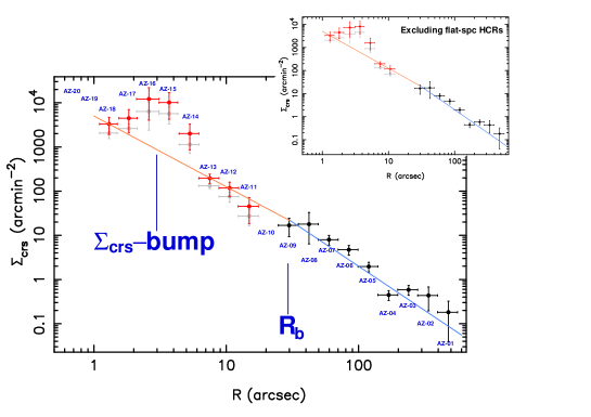
Figure 9: Radial distribution of the surface density of compact radio compact sources detected at the Galactic center. The red points are the surface density data $\Sigma^{*}_{\rm crs}$ corrected for a higher equivalent sensitivity cutoff at 5.5 GHz by multiplying the original 33-GHz surface density data, $\Sigma_{\rm crs}$ (light-grey points), by a correction factor, $\eta=2.4$, derived from the 33-GHz observations of the HCRs (see Appendix A of this paper). The black points mark the data of GCCRs observed at 5.5 GHz. In the annular zones around $R=3"$, a bump in $\Sigma_{\rm crs}$ is present. The orange line is the best fit using a power-law with an index $\Gamma=1.6\pm 0.2$ for the inner region outside of the bump at 1.5 - 7 arcsec; and the blue line indicates the least squares fitting to the steeper power law with $\beta=2.0\pm 0.2$ for the outer region. The break radius, $R_{b}$, is $\sim 30"$, or $\sim 1.2$ pc. The top-right inset shows the surface-density distribution of the HCRs excluding the flat-spectrum sources.

5.2 A dense group of HCRs and the radial distribution of their surface-density

The surface density of 110 GCCRs, located outside Sgr A West ($>1$ arcmin from Sgr A*) but within the RBZ ($<7.5$ arcmin from Sgr A*), is $\sim$0.6 counts arcmin^-2. This surface density is an order of magnitude greater than that of background extragalactic compact radio sources (e.g. Condon et al., 2012; Gim et al., 2019). The dense group of 64 HCRs, located within a radius of 13” from SgrA*, has a relatively higher surface density, with an average value of $\sim$500 counts arcmin^-2. We conclude that contamination of our sample by extragalactic background sources is very likely to be negligible.

In Appendix A, we developed a procedure to construct the surface-density ($\Sigma_{\rm crs}$) distribution of the radio compact sources (RCS) as function of the projected radial distance ($R$) from Sgr A*, including 64 HCRs at $R<13$” (this paper) and the 110 GCCRs outside Sgr A West (Zhao, Morris & Goss, 2020) as well as the Galactic center transient (GCT, see Zhao et al., 1992). Fig. 9 shows the radial distribution of the surface-density of the RCSs detected within the RBZ. Excluding the four data points related to a $\Sigma_{\rm crs}-$bump in the radial distance range between 1.5” and 7”, the surface-density distribution can be fitted with two power laws (see Fig. 8) as described by the “Nuker” law (Lauer et al., 1995; Genzel et al., 2003; Fritz et al., 2016; Schödel, 2018). In the inner region at $R<30$” but excluding the range between 1.5” and 7”, the surface-density distribution of the HCRs follows a power law:

$$\centering\Sigma_{\rm HCR}(R<30")\approx(5.0\pm 1.8)\times 10^{3}R_{\rm arcsec}^{-\Gamma}\leavevmode\nobreak\ \leavevmode\nobreak\ \leavevmode\nobreak\ \leavevmode\nobreak\ ({\rm arcmin^{-2}})\@add@centering$$ (1)

where the index $\Gamma=1.6\pm 0.2$. At large radii $R\geq 30$”, the surface-density distribution of the GCCRs shows a steeper power law:

$$\centering\Sigma_{\rm GCCR}(R\geq 30")\approx(2.0\pm 0.9)\times 10^{4}R_{\rm arcsec}^{-\beta}\leavevmode\nobreak\ \leavevmode\nobreak\ \leavevmode\nobreak\ \leavevmode\nobreak\ ({\rm arcmin^{-2}})\@add@centering$$ (2)

where $\beta=2.0\pm 0.1$. At $R\sim 30$”, the two power laws intersect. We note that the power-law distribution derived from HCRs is much steeper than that $\Gamma\sim 0.6$ of the stellar cusp determined with the $K_{\rm s}$ stars in magnitude range between 12.5 and 18.5 in the radial distance range between 1” and 50” (Gallego-Cano et al., 2018).

5.3 Candidate massive stellar remnants

5.3.1 Mass segregation

It has been known for several decades that the central parsec contains a large number of young massive stars (Krabbe et al., 1991, 1995; Paumard et al., 2001, 2006; Gillessen et al., 2009; Lu et al., 2009; Bartko et al., 2010; Lu et al., 2013), with $\sim$100 O and Wolf-Rayet (WR) stars confined within a radius of $\sim$0.4 pc (Genzel et al., 2003; Ghez et al., 2005). These stars are relatively young ($\leq 10$ Myr) and are orbiting Sgr A*, the supermassive black hole (SMBH) at the Galactic center. The early-type stars provide substantial UV photons to maintain the ionization of the gas within the central parsec (Zhao et al., 2010).

The stars in the central cusp apparently have a top-heavy present-day mass function (over-abundance of high-mass stars, see Bartko et al., 2010; Lu et al., 2013); and the fact that the orbits of many of them collectively define a coherent disk suggests that the young nuclear cluster may have originated via in situ star formation (Levin & Beloborodov, 2003; Levin, 2007; Nayakshin et al., 2007; Collin & Zahn, 2008). The process that formed the young nuclear cluster near the central black hole is likely to have been a recurring one. This process follows a limit cycle of activity wherein the star formation is a violent event coinciding with a heavy accretion episode onto the SMBH. Thus the inner disk is quickly disrupted and dissipated in the process. Following the disruption of the inner disk, continued migration of gas from the central molecular zone toward the center rebuilds the disk, eventually leading to the next star formation event (Morris, Ghez, & Becklin, 1999). With repeated instances of this cycle, the remnants of massive stars are produced and left in place to collect at the bottom of the Galaxy’s gravitational potential well. Furthermore, the more massive remnants, particularly stellar-mass black holes, will undergo mass segregation in the dense central star cluster, as a result of dynamical friction, and become even more concentrated toward the black hole (Bahcall & Wolf, 1976; Morris, 1993; Miralda-Escudé & Gould, 2000; Pfahl & Loeb, 2004; Freitag, Amaro-Seoane, & Kalogera, 2006; Alexander & Hopman, 2009; Merritt, 2010; Antonini & Merritt, 2012; Alexander et al., 2017; Generozov et al., 2018). The mass segregation may partially explain the intense flux of gamma rays and X-rays from the Galactic center caused by the possible presence of a large population of millisecond pulsars (MSPs) and cataclysmic variables (CVs), as suggested by (Arca-Sedda et al., 2018). The excess of GeV gamma rays toward the Galactic center may alternatively be explained by a high supernovae rate, leading to the production of neutron stars and ultimately to a MSP population (O’Leary et al., 2015, 2016; Calore et al., 2016).

In the case of stellar-mass BHs that are significantly more massive than the mean stellar mass expected for an evolved population, such heavier objects would migrate toward the center and be distributed in a compact cluster around the SMBH. The nature of the mass segregation depends on the relaxational coupling parameter $\Delta=4n_{\rm BH}M^{2}_{\rm BH}/\left[n_{\rm st}M^{2}_{\rm st}(3+M_{\rm BH}/M_{\rm st})\right]$ for black hole (BH) mass $M_{\rm BH}$ and spatial number density $n_{\rm BH}$ along with stellar (ST) mass $M_{\rm st}$ and spatial number density $n_{\rm st}$. The value of $\Delta$ is a measure of the importance of BH-BH scattering relative to BH-ST scattering for the dynamical friction process (Alexander & Hopman, 2009). Weak segregation occurs when $\Delta\gg 1$; and when $\Delta\ll 1$, the strong segregation applies. The latter case leads to a steeper slope in the 3D radial density distributions of BHs and a larger central concentration of BHs relative to that of stars: for power-law indices $\gamma_{\rm BH}$ and $\gamma_{\rm ST}$ for BHs and stars, respectively, $2\lesssim\gamma_{\rm BH}\lesssim 11/4$ and $3/2\lesssim\gamma_{\rm ST}\lesssim 7/4$ ($\gamma_{\rm BH}-\gamma_{\rm ST}\backsimeq 1$) (Alexander et al., 2017). Long-lived stellar populations usually have $\Delta<0.1$, and the Galactic center is expected to be strongly segregated (Morris, 1993). Alexander & Hopman (2009) have shown the effects of strong mass segregation on the density distribution of a model stellar population around Sgr A* (mass $M_{\rm SMBH}=4\times 10^{6}$ M_⊙); the modelled population includes main sequence stars (MS$\sim 1$ M_⊙) and stellar remnants, including white dwarfs (WD$\sim 0.6$ M_⊙), neutron stars (NS$\sim 1.4$ M_⊙) and black holes (BH$\sim 10$ M_⊙). Their study demonstrates that the heavier objects produce steeper density distributions via the mass segregation process.

We note that, in the radial range 0.04-1 pc, the power-law index of the 2D surface-density profile of the HCRs is $\Gamma_{\rm HCR}=1.6\pm 0.2$ (this paper) which is much greater than the corresponding value of $\Gamma_{K_{\rm s}}$ for the $K_{\rm s}$ stars in the same radial range (Gallego-Cano et al., 2018). The difference between the power-law indices ($\Gamma_{\rm HCR}-\Gamma_{K_{\rm s}}$) is $\sim$1. The flat power-law profile for $K_{\rm s}$ stars provides evidence for the presence of a dynamically relaxed stellar cusp at the Galactic center (Gallego-Cano et al., 2018; Schödel, 2018). On the other hand, with the arguments presented in the previous paragraph, the dense group of HCRs reported in this paper, with its much steeper radial distribution (see Fig. A2) than that of the faint $K_{\rm s}$ stars, could represent a population of massive stellar remnants that are mass-segregated in the nuclear star cluster at the Galactic center. The HCRs are associated with active massive stellar remnants having relatively higher radio luminosities. The surface density profile of the HCRs (see Fig. A2) may be subject to change when a deeper radio survey is carried out with a much lower flux density cutoff. Nevertheless, the results from our study of HCRs in the central parsec provides evidence consistent with the presence of a distribution of massive stellar remnants that is a steep function of the radial distance from Sgr A*.

In addition, if the massive stellar remnants associated with the HCRs had migrated inward via dynamical friction, the bump in surface density, $\Sigma_{\rm HCR}$, at 0.1-0.3 pc could be attributed to an accumulation in that radial range since the dynamical friction force acting on a massive object ceases at roughly half the radius of the stellar core ($\sim 0.25$ pc) (Merritt, 2010). A maximum in the density profile of massive remnants is also predicted to occure at $\sim 0.2$ pc at a time $>$1 Gyr in a dynamical evolution model, and the bump slowly grows and migrates inward due to the friction produced by fast-moving stars inside these radii (Antonini & Merritt, 2012). The $\Sigma_{\rm HCR}$-bump may serve as an additional observational signature of massive stellar remnants as a consequence of stellar dynamical processes in galactic nuclei.

5.3.2 Radiation spectrum

Hailey et al. (2018) recently reported the identifications of a dozen low-mass back hole X-ray binary candidates within the central parsec, implying the presence of a large population of X-ray binaries and isolated black holes residing within that volume (Generozov et al., 2018). Most of them are in a quiescent state. X-ray and radio flares and outbursts from these stellar remnants have been discovered over the past three decades, such as the magnetar SGR J1745-2900 (Kennea et al., 2013; Rea et al., 2020; Eatough et al., 2013; Shannon & Johnston, 2013; Torne et al., 2015, 2017), the microquasar of the X-ray transient XJ174540.0290031 (Muno et al., 2005; Bower et al., 2005; Zhao et al., 2009) and the Galactic center transient (GCT, see Zhao et al., 1992) as well as the X-ray PWN candidate G359.95-0.04 (Baganoff et al., 2003; Wang et al., 2006; Muno et al., 2008) which is likely powered by a neutron star.

With a flux-density range bewteen $\sim$0.1 and a few mJy at 33 and 44.6 GHz, the HCRs appear to be candidate radio counterparts of the old massive stellar remnants produced in the end of stellar evolution as expected. Most of them are in a quiescent state. Although their progenitors and ages are unknown, the 38 steep spectrum HCRs determined from the JVLA observation at Ka and Q bands provide important clues on the nature of the radio radiation, affirming nonthermal radiation with a steep power law in the distribution of relativistic electrons. The nonthermal emission could be produced by synchrotron jets or outflows that were launched from the compact stellar remnants powered by accretion from the dense, local medium.

As described above, one of the 17 inverted-spectrum HCRs is the GC magnetar, SGR J1745-2900, which shows high-frequency pulses up to 291 GHz (Torne et al., 2017). The continuum emission from this magnetar has been firmly detected at high radio frequencies up to 340 GHz (Tsuboi et al., 2017, and this paper). The inverted-spectrum of the mm-component of a magnetar towards the submillimeter appears to be a remarkable radio wavelength signature, as predicted by the dynamical model of Beloborodov (2013) using a persistent flow of electron-position plasma. The configuration of the magnetosphere of magnetars, created by enforced electric current and radiative drag together, is subject to two-stream instability. Consequently a relatively hard radio spectrum that is predicted to emerge, perhaps extending to IR/optical/UV wavelengths, and is expected to be generated because the instability leads to a large plasma density, and thus a large plasma frequency (Beloborodov, 2013). The theory also predicts a large electric current associated with the radio-submillimeter emission from magnetars (Beloborodov, 2013), producing a bright radiation beam much broader than the typical pulse width of normal pulsars with similar periods (Camilo et al., 2006, 2007). A valuable next step will be to use this theory to formulate predicted shapes of radio spectra and pulse profiles of magnetars for comparison with observations.

The suggestion has been made that pulsars formed at or near the Galactic center might mostly to be magnetars, given the rather highly magnetized interstellar medium of the GC region that could produce highly magnetized massive stars. Subsequently, strongly magnetized neutron star remnants form because of the collapse of stellar core and concentration of the flux-frozen magnetic field (Dexter & O’Leary, 2014; Morris, 2014). However, because the magnetic flux within the core of a massive star as well as within a neutron star can undergo considerable evolution owing, for example, to dynamo action occurring inside the star and the neutron star, (e.g., Duncan & Thompson, 1992; Thompson & Duncan, 1993), this scenario remains rather speculative. In any case, the discovery of SGR J1745-2900 makes the central parsec a potentially interesting region to search for new magnetars. Although the recent formation of a large number of massive stars there could have led to a population of neutron star remnants, if those remnants are predominantly highly magnetized, then, as with magnetars in general, they would have short lifetimes as pulsars ($\sim$ 10${}^{3}-10^{5}$ yrs) because of the powerful spindown torque associated with the interaction of the neutron star’s magnetic field with the plasma in its environment (Harding et al., 1999; Espinoza et al., 2011; Dexter & O’Leary, 2014; Kaspi & Beloborodov, 2017). The time period during which a magnetar is an observable pulsar is therefore more than two orders of magnitude shorter than the lifetime of the massive stars observed in the young nuclear cluster ($\sim$2 - 10 Myrs). So we might therefore expect only a few (or zero) magnetars to be found as pulsars at any one time in the central parsec if the above speculation that massive GC stars produce highly magnetized remnants is correct. Indeed, in addition to the scatter-broadening that occurs primarily at longer radio wavelengths, the short lifetime of strongly magnetized pulsars could be the main explanation for the rarity of pulsars at the Galactic center. The remaining open question is whether magnetars remain detectable as point radio continuum sources even after they have spun down to the point at which they can no longer be detectable as pulsars. If so, then we might consider that some of the HCRs are in that category.

The inverted spectrum towards short wavelengths found in 1E1547.0-5408 (Chu et al., 2021) in addition to SGR J1745-2900 is also consistent with the prediction of spectral hardening at short radio wavelengths from the two-stream instability model (Beloborodov, 2013). The combination of the inverted spectrum, high variability and high polarization – nearly 100% for the degree of linear polarization and 15% for circular polarization (Eatough et al., 2013) – appears to be unique to magnetars.

Of course, both the inverted and flat spectra of HCRs can also be interpreted as self-absorbed synchrotron emission from X-ray binaries in the hard state when the radiation is dominated by the emission from the corona of the compact object (Coriat et al., 2011).

6 Conclusion

Following our 5.5-GHz JVLA survey of the Galactic center compact radio sources (GCCRs) within the radio bright zone, we have continued to explore Sgr A West using Ka- and Q-band data obtained by the JVLA in its A-configuration. At an angular resolution of 0.05 arcsec, we detected a dense group of hyper-compact (¡0.1”) radio sources (HCRs) within the central parsec of the Galaxy. Based on a conservative 15$\sigma$ flux-density threshold, corresponding to 150 $\mu$Jy at 33 GHz, we cataloged 64 HCRs with their J2000 equatorial coordinates, flux densities at 33 and 44.6 GHz, angular sizes derived from 2D Gaussian fitting, and spectral index, $\alpha_{44.6/33}$. HCR49 is double.

The surface-density distribution, $\Sigma_{\rm HCR}(R),$ shows a local enhancement or a density bump in the projected radial distance ($R$) range 1.5”–7” superimposed on a power-law distribution with an index of $\Gamma=1.6\pm 0.2$. The steeper profile of the HCRs relative to that of the nuclear stellar cluster might result from the concentration of massive stellar remnants by mass segregation.

The 65 HCRs divide into three spectral sub-types: 38 steep-spectrum ($\alpha_{44.6/33}\leq-0.5$), 10 flat-spectrum ($-0.5$ ¡ $\alpha_{44.6/33}\leq$ 0.2), and 17 inverted-spectrum sources ($\alpha_{44.6/33}$ ¿ 0.2). Our statistical analysis shows that the distribution of the steep-spectrum HCRs in Log(S[mJy] can be fitted to a Gaussian with a mean of $\mu=-0.35$ (corresponding to 0.45 mJy) and a standard deviation of $\sigma=0.22$. We suggest that the steep-spectrum HCRs be regarded as candidates for a population of stellar remnants acting as nonthermal compact radio sources powered by accretion onto neutron stars and stellar-mass black holes, with the accreted matter supplied either by a binary companion or by a dense portion of the interstellar medium.

The inverted-spectrum HCRs show a rising spectrum towards high frequencies. Five of the 17 inverted-spectrum HCRs have compact IR counterparts, suggesting that they are associated with the ionized stellar wind outflows from hot, massive stars. A portion of the inverted-spectrum HCRs may consist of X-ray binaries in the hard state, when the self-absorbed synchrotron emission is dominated by the corona of the compact object. The GC magnetar, SGR J1745-2900, belongs to the inverted-spectrum sub-type. Based on our analysis of 91 flux-density measurements of SGR J1745-2900 observed with the JVLA, ALMA and ATCA, we find that two distinguishable spectral components contribute to the averaged spectrum, separated at the transition frequency $\nu_{t}\sim 30$ GHz. The cm-component is fitted to a power-law with a steep spectral index $\alpha_{\rm cm}=-1.5\pm 0.6$ while the mm-component shows the inverted spectrum $\alpha_{\rm mm}=1.1\pm 0.2$. Our consolidation of the spectrum from the interferometer array data is in good agreement with earlier results based on single-dish observations (Torne et al., 2017).

In addition, we reduced 225-GHz ALMA data observed with a FWHM beam of 0.024”$\times$0.017” on ten individual days within two weeks in October, 2017. SGR J1745-2900 was detected with a signal-to-noise ratio of $\sim$70 at flux densities varying widely between 0.79 and 5.60 mJy on day-to-day timescales. An index of relative variability $\mathscr{RV}\approx$ 6 is found for SGR J1745-2900, which compares with $\mathscr{RV}\approx$ 0.2 for the more moderately variable Sgr A*, derived from the same ALMA observations.

Collecting a total of 161 individual flux-density measurements of SGR J1745-2900 at radio wavelengths from prior published literature and this paper, we binned data into 100-day bins along the time axis for both cm- and mm-components separately, starting from the outburst on April 23, 2013 (MJD 56406). The radio light curves with bin-averaged flux density are compared with the X-ray light curve observed with Chandra (Rea et al., 2020). Except for the appreciable short-timescale variability at millimeter wavelengths, the long-term trend at both centimeter and millimeter wavelengths is a slow, but erratic, decrease in radio power, in contrast to the smoothly decreasing trend in X-ray luminosity.

Because many HCRs are candidates for being remnants of massive stars, we considered the origin and fate of such remnants, and speculated on the possible reasons for the difficulty of finding pulsars there. Neutron stars formed within the relatively highly magnetized central molecular zone of the Galaxy could themselves inherit sufficient magnetic flux that they are mostly born as magnetars. In that case, their ultra-strong magnetic fields (10¹⁴ - 10¹⁶ G), acting on plasma trapped in their magnetospheres, apply a spin-down torque that causes them to have relatively short lifetimes as detectable pulsars ($10^{3}\leavevmode\nobreak\ -\leavevmode\nobreak\ 10^{5}$ yr) compared to normal pulsars.

If the inverted spectrum towards high frequencies found in SGR J1745-2900 and 1E1547.0-5408 is a common characteristic of active magnetars, the high-frequency bands (Ka and Q) of the JVLA and all the ALMA and SMA bands open a practical window for studying magnetars. Also, dynamical information on the HCRs can be acquired with high-precision proper motion data that can be obtained with repeated JVLA and ALMA observations. Such measurements will supply strong constraints on the candidacy of the HCRs as massive stellar remnants at the Galactic center.

A Density distribution of HCRs and GCCRs

The stellar density distribution in the Galactic center can be fitted by two power laws (e.g., Genzel et al., 2003; Fritz et al., 2016), with a flat inner component and a steeper component at large projected radii (Schödel, 2014, 2018). Usually, the projected surface density can be described by the “Nuker” profile with two slopes (Lauer et al., 1995):

$$\centering\Sigma(R)=\Sigma(R_{b})2^{(\beta-\Gamma)/\alpha}\left(R_{b}\over\/R\right)^{\Gamma}\left[1+\left(R\over\/R_{b}\right)^{\alpha}\right]^{(\Gamma-\beta)/\alpha)}\@add@centering$$ (A1)

where $\Sigma(R_{b})$ is the surface density at the break radius $R_{b}$ that divides the profile into two power laws. At a small radius $R\ll R_{b}$, $\Sigma(R)\sim\/R^{-\Gamma}$, usually describing the cusp in the distribution of old stellar population. For $R\gg R_{b}$, $\Sigma(R)\sim\/R^{-\beta}$, fitting to the outer power law, which is usually steeper than that of the cusp (Lauer et al., 1995). The break radius $R_{b}$ corresponds both to the point at which the slope is the mean of $\beta$ and $\Gamma$ and to the radius of maximum curvature of the distribution in the log₁₀($R$)-log₁₀($\Sigma(R_{b})$) coordinate system.

In this section, we present the algorithm that we developed to derive the distribution of the surface density ($\rm\Sigma_{\rm crs}$) for the compact radio sources (CRS) as function of the projected radial distance from Sgr A*.

A.1 Algorithm

First, the radio bright zone (RBZ) is divided into 20 annular zones (AZ), each of them bounded by two rings at outer and inner radii, $R(i)$ and $R(i+1)$:

$$\centering R(i)=2^{-0.5i}R_{\rm RBZ},\@add@centering$$ (A2)

where $i=0,1,2...,19\leavevmode\nobreak\ {\rm and}\leavevmode\nobreak\ 20$ and $R_{\rm RBZ}$ is the outer radius of the radio bright zone (RBZ). Fig. A1 shows the 20 annular zones along with the distribution of GCCRs and HCRs in the RBZ (Fig. A1a), Sgr A West (Fig. A1b) and the central parsec (Fig. A1c). The radius of the outer ring, $R(0)=R_{\rm RBZ}$, corresponds to the largest radius within which we searched the GCCRs with a 10-$\sigma$ cutoff due to the JVLA primary beam at 5.5 GHz. The radius of the most inner ring, $R(20)=0.55"\approx\theta_{\rm FWHM}$, is approximately the size of FWHM beam at 5.5 GHz. The zone AZ-10 marks the boundary, within which we found 64 HCRs with the JVLA A-array observations at 33 and 44.6 GHz (this paper). Outside this boundary, 110 GCCRs are found from the JVLA A-array observations at 5.5 GHz (Zhao, Morris & Goss, 2020).

Then, we counted the CRS in each of the AZs by creating a grid function $crs(j,k)$ for each of the CRSs, where $k$ is the annular zone ID from 1 to 20 and $j$ is the CRS source ID within an AZ. For given a specific grid cell ($j,k$), a unit value is assigned, i.e. $crs(j,k)=1$. Given a $k$, the AZ-ID, the number of sources in an annular zone is then derived by summing over $j$:

$$\centering N(k)=\sum_{j}{crs(j,k)}.\@add@centering$$ (A3)

In addition, we also created grid functions of $s(j,k)$ and $\sigma(j,k)$ for flux-density and uncertainty, respectively. Corresponding to a specific source ID: ($j,k$), the values of flux density and 1-$\sigma$ uncertainty of the CRS are assigned to $s(j,k)$ and $\sigma(j,k)$. The accumulated flux density of CRS in an annular zone can be determined:

$$\centering S(k)=\sum_{i=1}^{N(k)}{s(j,k)},\@add@centering$$ (A4)

and

$$\centering\sigma(k)=\sqrt{\sum_{j=1}^{N(k)}{\sigma(j,k)^{2}}}.\@add@centering$$ (A5)

We note that, for the GCCRs, $s(j,k)$ and $\sigma(j,k)$ correspond to the mean and 1-$\sigma$ error of the mean, which are determined with the measurements from the three-epoch observations at 5.5 GHz (Zhao, Morris & Goss, 2020). For the HCRs, we used Ka-band flux density and 1-$\sigma$ error at 33 GHz (this paper). The area for the $k$-th AZ can be computed:

$$\centering A(k)=\pi\left[R(k)^{2}-R(k+1)^{2}\right].\@add@centering$$ (A6)

Furthermore, we also estimated a flux-density-based CRS counts $N_{S}(k)$:

$$\centering N_{S}(k)={S(k)\over S_{\mu,5.5\leavevmode\nobreak\ {\rm GHz}}},\@add@centering$$ (A7)

for $k<11$ and

$$\centering N_{S}(k)={S(k)\over S_{\mu,33\leavevmode\nobreak\ {\rm GHz}}}\@add@centering$$ (A8)

for $k\geq 11$. Here $S_{\mu,5.5\leavevmode\nobreak\ {\rm GHz}}$ and $S_{\mu,33\leavevmode\nobreak\ {\rm GHz}}$ are the mean flux-density values for the GCCRs at 5.5 GHz and HCRs at 33 GHz.

Given the sensitivity cutoff and the variability of the CRSs, the direct source counts $N(k)$ represents a lower limit of the $k$-th AZ. The flux-density-based CRS counts $N_{S}(k)$ is usually greater than the direct source counts, i.e., $N_{S}(k)>N(k)$. Thus, using the averaged values of $\displaystyle{\left[N_{S}(k)+N(k)\right]/2}$ we derived the surface density of CRSs as a function of radius from Sgr A*:

$$\centering\Sigma_{\rm crs}(k)=\displaystyle{\left[N_{S}(k)+N(k)\right]\over 2A(k)}.\@add@centering$$ (A9)

The uncertainty of surface density is estimated as well:

$$\centering\Delta_{\Sigma_{\rm crs}}(k)=\displaystyle{\left[N_{S}(k)-N(k)\right]\over 2A(k)}.\@add@centering$$ (A10)

where $k=1,2,3,$ … and 20. Thus, the upper and lower limits in surface density correspond to the flux-density-based density ($N_{S}(k)/A(k)$) and the actual-source-counted density ($N(k)/A(k)$), respectively.

We then calculated the mean radius given the $k$-th annular zone:

$$\centering R_{\rm AZ}(k)={{R(k)+R(k+1)}\over 2},\@add@centering$$ (A11)

and the uncertainty, or more properly half of the annular zone width:

$$\centering\Delta_{R_{\rm AZ}}(k)={{R(k)-R(k+1)}\over 2},\@add@centering$$ (A12)

where $R(k)$ is defined in Eq.(A1) and $k=1,2,3,$ … and 20.

Fig. A2 shows the distribution of the surface density of CRSs $\Sigma_{\rm crs}(R)$ as a function of radial distance ($R$) from Sgr A*. The black symbols represent the data at a large projected radius ($R>13$”), determined from the JVLA observations at 5.5 GHz (Zhao, Morris & Goss, 2020) while the symbols for the inner annular zones ($R\leq 13$”) mark the data derived from the Ka-band observations at 33 GHz. We note that the CRS counts, as well as the surface density $\Sigma_{\rm crs}$ (light-grey symbols in Fig. A2), may be underestimated within the inner annular zone (AZ=11 - 20) due to the fact that the data HCRs observed at 33 GHz corresponds to a higher effective cutoff limit at 5.5 GHz since most of the HCRs have a steep spectrum. With an averaged spectral index $\alpha_{\rm HCRs}=-0.42\pm 0.12$ using all 64 HCRs’ data, we converted the 33-GHz flux densities to 5.5-GHz. The equivalent cutoff limit for the inner AZs is about twice as high as the limit searched for GCCRs in the RBZ (Zhao, Morris & Goss, 2020). So, we multiplied the surface density of the inner AZ(k$\geq$11) by a correction factor:

$$\centering\eta=(5.5/33)^{\alpha_{\rm HCR}}\left(\sigma_{33}\over\sigma_{5.5}\right)\approx 2.4,\@add@centering$$ (A13)

assuming that the HCR counts are inversely proportional to the cutoff value in flux density. The corrected surface density is then computed:

$$\centering\Sigma^{*}_{\rm crs}=\eta\Sigma_{\rm crs}\@add@centering$$ (A14)

as indicated with the red symbols which appear to be aligned better with the surface density data of the outer radii obtained from the observations at 5.5 GHz.

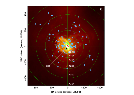
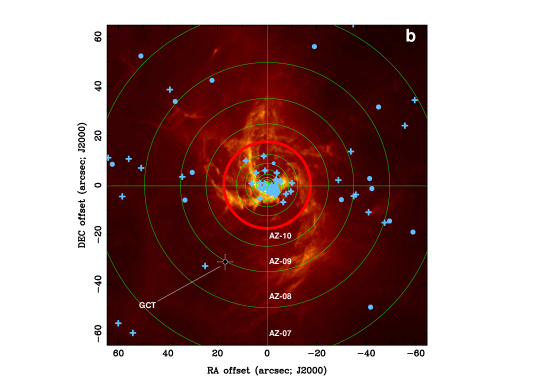
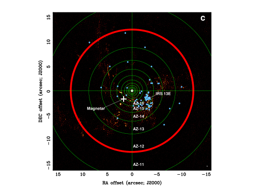
Figure A1: The radio bright zone (RBZ) is divided into 20 annular zones (AZ) along the radial direction from Sgr A*. Spatial distribution of GC compact radio sources or GCCRs (light blue symbols, crosses for variables and dots for non-variables) in annular zones is displayed over the RBZ (AZ 1 - 6) (top panel: Fig. A1a) and SgrA West (AZ 7-11) (middle panel: Fig. A1b). The HCRs (light blue dots) are distributed in the central parsec (AZ 12-20) (bottom panel: Fig. A1c). The thick red ring marks the 11-th ring (Eq. A2), $R(11)=13$”, $\sim 0.5$ pc. In Figs. A1a and A1b, the symbol of a black cross-dot marks the Galactic center transient, the GCT (Zhao et al., 1992). The magnetar J1745-2900 and IRS 13E are labelled in Fig. 1Ac.

A.2 Power-law fit to the $\Sigma_{\rm crs}$ distribution

The surface-density $\Sigma_{\rm crs}$ data at large radii (from AZ01 to AZ09) can be described by a power law while the data at small radii (from AZ10 to AZ18) show a bump ($\Sigma_{\rm crs}$-bump), indicating a locally enhanced source density $\Sigma_{\rm crs}$ at the radial distance range of $R=1.5$”$-7.0$” (from AZ-17 to AZ-14) superimposed on a slope. We made a linear regression fit to a function:

$$\centering Log_{10}(\Sigma_{\rm crs})=a_{\rm GCCR}-\beta\/Log_{10}(R),\@add@centering$$ (A15)

using the outer nine AZ’s data points (GCCRs) with a weight of $wt(i)=\Delta^{-2}_{\Sigma_{\rm crs}}(k)$. The best fit derived from the least squares regression (LSR), as indicated by a straight blue line in Fig. A2, gives a power law function $\Sigma_{\rm crs}\propto\/R^{-\beta}$ ($R>13$”) with $\beta=2.0\pm 0.1$ and $a_{\rm GCCR}=4.3\pm 0.2$.

For the inner eight annular-ring data (HCRs), we excluded the four data points that are involved in the $\Sigma_{\rm crs}$-bump (from AZ14 to AZ17) and fit the remaining four data points with a linear function:

$$\centering Log_{10}(\Sigma_{\rm crs})=a_{\rm HCR}-\Gamma\/Log_{10}(R).\@add@centering$$ (A16)

Based on a least-squares fitting, we derived $\Sigma_{\rm crs}\propto\/R^{-\Gamma}$ ($R\leq 13$”) with $\Gamma=1.6\pm 0.2$ and $a_{\rm HCR}=3.7\pm 0.2$, as indicated with the straight orange line in the logarithmic plot (Fig. A2a). The $\Sigma_{\rm crs}$-bump is characterized by the high surface-density zones AZ15 and AZ16; the former contains the GC magnetar J1745-2900 and the latter is associated with IRS 13E. We note that the surface brightness in the diffuse Br$\gamma$ narrow band filter image (Fig. 6a of Schödel (2018)) also shows a bump in the range of radius between $R=1.5$” and $7.0$”, suggesting that the counts of CRSs in the radial range may be partially caused by the local hyper compact HII sources associated with younger massive stellar objects. However, excluding the flat-spectrum HCRs, the $\Sigma_{\rm crs}-$bump is also present (see Fig. A2b). We further checked the distribution only with the steep-spectrum HCRs and found that the $\Sigma_{\rm crs}-$bump is still present in the radial range between $R=1.5$” and $7.0$” (see Fig. A2c).

Due to a small number of data points and at least four free parameters in the “Nuker” model of Eq(A1), we made no attempt to fit the entire curve for deriving the break radius $R_{b}$. However, from the intersection between the two straight lines of Eq(A15) and Eq(A16), we found an approximate break radius $R_{b}\approx 30$”, or 1.1 pc, which appears to correspond to the radius of the ionized region. Therefore, in the main text, we use $R_{b}=30$” as the break radius that separates the two distinctive power-law distributions.

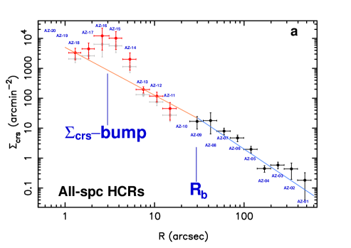
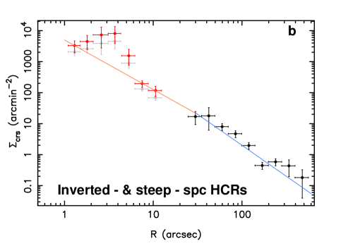
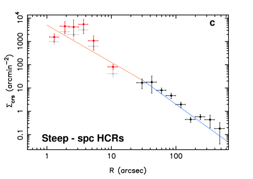
Figure A2: Radial distribution of surface density of radio compact sources detected at the Galactic center. The red points are the surface density data $\Sigma^{*}_{\rm crs}$ corrected for a higher equivalent sensitivity cutoff at 5.5 GHz by multiplying a correction factor $\eta=2.4$ (see Eqs. A13 and A14) to the original 33-GHz surface density data $\Sigma_{\rm crs}$ (light-grey points) derived from the 33-GHz observations of the HCRs (this paper). The black points mark the data of GCCRs observed at 5.5 GHz. In the annular zones around $R=3"$, a bump in $\Sigma_{\rm crs}$ is present. The orange line shows the best fitting to the power-law function with $\Gamma=1.6\pm 0.2$ for the inner region; and the blue line indicates the least squares fitting to the steeper power law with $\beta=2.0\pm 0.2$ for the outer region. The break radius $R_{b}$ is $\sim 30"$, or $\sim 1.2$ pc. Three panel show the surface-density distributions for the three combinations of spectrum classes of HCRs: (a) inclduing all the HCRs, (b) excluding the flat-spectrum HCRs, and (c) only including inverted HCRs.

References

- Alexander et al. (2017) Alexander, T. 2017, ARA&A, 55, 1
- Alexander & Hopman (2009) Alexander, T. & Hopman 2009, ApJ, 697, 1861
- Antonini & Merritt (2012) Antonini, F. & Merritt, D. 2012, ApJ, 745, 83
- Arca-Sedda et al. (2018) Arca-Sedda, M., Kocsis, B. & Brandt, T. D. 2018, MNRAS, 479, 900
- Bahcall & Wolf (1976) Bahcall, J. N. & Wolf, R. A. 1976, ApJ, 209, 214
- Baganoff et al. (2003) Baganoff, F. K. et al. 2003, ApJ, 591, 891
- Bartko et al. (2010) Bartko, H., Martins, F., Trippe, S. et al. 2010, ApJ 708, 834
- Beloborodov (2013) Beloborodov, A. M. 2013, ApJ, 777, 114
- Bonato et al. (2018) Bonato, M., Liuzzo, E., Giannetti, A. et al. 2018, MNRAS, 478, 1512
- Bower et al. (2005) Bower, G. C., Roberts, D. A., Yusef-Zadeh, F., Backer, D. C., Cotton, W. D., Goss, W. M., Lang, C. C., & Lithwick, Y. 2005, ApJ, 633, 218
- Bower et al. (2014) Bower, G. C., Deller, A., Demorest, P. et al. 2014, ApJ, 780, L2
- Bower et al. (2015/16) Bower, G. C. et al. 2015 ApJ, 798, 120 & 2016, ApJ 821, 133
- Briggs (1995) Briggs, D. S. 1995, PhD Thesis: “HIGH FIDELITY DECONVOLUTION OF MODERATELY RESOLVED SOURCES”, NRAO & NM Tech., https://casa.nrao.edu/Documents/Briggs-PhD.pdf
- Calore et al. (2016) Calore, F., Di Mauro, M., Donato, F., Hessels, J.W.T. & Weniger, C. 2016, ApJ 827, 143
- Camilo et al. (2006) Camilo, F., Ransom, S. M., Halpern, J. P., et al. 2006, Nature, 442, 892
- Camilo et al. (2007) Camilo, F., Ransom, S. M., Halpern, J. P., & Reynolds, J. 2007, ApJL, 666, L93
- Chu et al. (2021) Chu, Che-Yen, Ng, C. -Y., Kong, Albert K. H., Chang, Hsiang-Kuang 2021, NMRAS, 503, 1214
- Clark et al. (2021) Clark, J. S., Patrick, L. R., Najarro, F., Evans, C. J. & Lohr, M. 2021 å, 649, 43
- Collin & Zahn (2008) Collin, S. & Zahn, J.-P. 2007, A&A 477, 419
- Condon et al. (2012) Condon, J. J., Cotton, W. D., Fomalont, E. B., et al. 2012, ApJ, 758, 23
- Coriat et al. (2011) Coriat, M., Corbel, S., Prat, L. et al. 2011, MNRAS, 414, 677
- Dexter & O’Leary (2014) Dexter, J. & O’Leary, R. M. 2014, ApJL, 783, L7
- Dong, Wang & Morris. (2012) Dong, H., Wang, Q.D. & Morris, M.R. 2012, MNRAS 425, 884.
- Duncan & Thompson (1992) Duncan, R.C. & Thompson, C. 1992, ApJL 392, L9
- Eatough et al. (2013) Eatough, R. P., Falcke, H., Karuppusamy, R., et al. 2013a, Nature, 501, 391.
- Eatough et al. (2021) Eatough, R.P., Torne, P., Desvignes, G. et al. 2021, MNRAS, 507, 5053.
- Espinoza et al. (2011) Espinoza, C.M., Lyne, A.G., Kramer, M., Manchester, R.N. & Kaspi, V.M. 2011, ApJL, 741, L13
- Freitag, Amaro-Seoane, & Kalogera (2006) Freitag, M., Amaro-Seoane, Pau, & Kalogera, V. 2006, ApJ 649, 91
- Fritz et al. (2016) Fritz, T. K. et al. 2016, ApJ, 821, 44
- Gallego-Cano et al. (2018) Gallego-Cano, E., Schödel, R., Dong, H., et al. 2018, A&A 609, A26.
- Gelfand et al. (2017) Gelfand, J. D. et al. 2017, ApJ, 850, 53
- Generozov et al. (2018) Generozov, A., Stone, N. C., Metzger, B. D. & Ostriker, J. P. 2018, MNRAS 478, 4030
- Genzel et al. (2003) Genzel, R., Schödel, R., Ott, T. et al. 2003, ApJ, 594, 812
- Ghez et al. (2005) Ghez, A. M., Salim, S., Hornstein, S. D., et al. 2005, ApJ, 620, 744
- Gillessen et al. (2009) Gillessen, S., Eisenhauer, F., Trippe, S., et al. 2009, ApJ, 692, 1075
- Gim et al. (2019) Gim, H. B., Yun, M. S., Owen, F. N., et al. 2019, ApJ, 875, 80
- Hailey et al. (2018) Hailey, C. J., Mori, K., Bauer, F. E., et al. 2018, Nature 256, 70
- Harding et al. (1999) Harding, A.K., Contopoulos, I. & Demosthenes, K. 1999, ApJL 525, L125
- Kaspi & Beloborodov (2017) Kaspi, V.M. & Beloborodov, A.M. 2017, ARA&A55, 261
- Kennea et al. (2013) Kennea, J. A., Burrows, D. N., Kouveliotou, C., et al. 2013, ApJL, 770, L24
- Krabbe et al. (1991) Krabbe, A., Genzel, R., Drapatz, S. & Rotaciuc, V. 1991, ApJL 382, L19
- Krabbe et al. (1995) Krabbe, A., Genzel, R., Eckart, A. et al. 1995, ApJL 447, L95
- Kramer et al. (1998) Kramer, M., Xilouris, K. M., Lorimer, D. R., et al. 1998, ApJ, 501, 270
- Lauer et al. (1995) Lauer, T. R., Byun, Y.-I., Dresseler, A., et al. 1995, ApJ, 110, 2622
- Lazio & Cordes (1998) Lazio, T. & Cordes, J. 1998, ApJ 505, 715
- Levin & Beloborodov (2003) Levin, Y. & Beloborodov, A.M. 2003, ApJL 590, L33
- Levin (2007) Levin, Y. 2007, MNRAS, 374, 515
- Lu et al. (2009) Lu, J. R., Ghez, A. M., Hornstein, M., et al. 2009, ApJ, 690, 1463
- Lu et al. (2013) Lu, J. R., Do, T., Ghez, A. M., et al. 2013, ApJ, 764, 155
- Manchester et al. (2005) Manchester, R. N., Hobbs, G. B., Teoh, A. and Hobbs, M. 2005, AJ, 129, 1993
- Merritt (2010) Merritt D. 2010, ApJ, 718, 739
- Miralda-Escudé & Gould (2000) Miralda-Escudé, J. & Gould, A. 2000, ApJ, 545, 847
- Mori et al. (2013) Mori, K., Gotthelf, E. V., Zhang, S. et al. 2013, ApJL, 770, L23
- Morris (1993) Morris, M. R. 1993, ApJ, 408, 496
- Morris, Ghez, & Becklin (1999) Morris, M., Ghez, A.M. & Becklin, E.E. 1999, AdSpR 23, 959
- Morris (2014) Morris, M. R. 2014, in “Lessons from the Local Group”, Springer, p391 (arXiv 1406.7859)
- Morris et al. (2017) Morris, R. M., Zhao, Jun-Hui & Goss, W. M. 2017, ApJL, 850, L23
- Muno et al. (2005) Muno, M. P., Pfahl, E., Baganoff, F. K., Brandt, W. N., Ghez, A., Lu, J., & Morris, M. R. 2005, ApJ, 622, L113
- Muno et al. (2008) Muno, M. P., Baganoff, F. K., Brandt, W. N., et al. 2008, ApJ, 673, 251
- Nayakshin et al. (2007) Nayakshin, S., Cuadra, J. & Springel, V. 2007, MNRAS 379, 21
- O’Leary et al. (2015) O’Leary, R. M., Kistler, M. D., Kerr, M. & Dexter, J. 2015, arXiv:1504.02477v1
- O’Leary et al. (2016) O’Leary, R. M., Kistler, M. D., Kerr, M. & Dexter, J. 2016, arXiv:1601.05797v2
- Panagia & Felli (1975) Panagia, N. & Felli, M. 1975, A&A, 39, 1
- Paumard et al. (2001) Paumard, T., Maillard, J.P., Morris, M., & Rigaut, F. 2001, A&A, 366, 466
- Paumard et al. (2006) Paumard, T., Genzel, R., Martins, F., et al. 2006, ApJ, 643, 1011
- Perley & Butler (2017) Perley, R. A. & Bulter, B. J. 2017, ApJS, 230, 7
- Pfahl & Loeb (2004) Pfahl & Loeb 2004, ApJ, 615, 253
- Porquet et al. (2005) Porquet, D., Grosso, N., Belanger, G., Goldwurm, A., Yusef-Zadeh, F., Warwick, R. S., & Predehl, P. 2005, A&A, 443, 571
- Rau & Cornwell (2011) Rau, U. & Cornwell, T. J. 2011, AA, 532, A71
- Rea et al. (2020) Rea, N., et al. 2020, ApJ, 894, 159
- Rea et al. (2013) Rea, N., Esposito, P., Pons, J. A. et al. 2013, ApJL, 773, L34
- Reid & Brunthaler (2014) Reid, M. J. & Brunthaler, A. 2004, ApJ, 616, 872
- Schödel (2014) Schödel, R., Feldmeier, A., Kunneriath, D., et al. 2014, A&A, 566, A47
- Schödel (2018) Schödel, R., Gallego-Cano, E., Dong, H. et al. 2018, A&A, 609, A27
- Shannon & Johnston (2013) Shannon, R. M. & Johnston, S. 2013, MNRAS, 435, L29
- Spitler et al. (2014) Spitler, L. G., Lee, K. J., Eatough, R. P., et al. 2014, ApJ, 780, L3
- Thompson, Moran & Swenson (2017) Thompson, A. R., Moran, J. M. & Swenson Jr., G. W. 2017, Interferometry and Synthesis in Radio Astronomy, Third Edition, Springer, Switzerland
- Thompson & Duncan (1993) Thompson, C. & Duncan, R.C. 1993, ApJ 408, 194
- Torne et al. (2015) Torne, P., Eatough, R. P., Karuppusamy, R. et al. 2017, MNRAS, 451, L50
- Torne et al. (2017) Torne, P., Desvignes, G., Eatough, R. P. et al. 2017, MNRAS, 465, 242
- Tsuboi et al. (2017) Tsuboi, Masato, Kitamura, Yoshimi, Tsutsumi, Takahiro et al. 2017, ApJL, 850, L5
- Tsuboi et al. (2019) Tsuboi, Masato, Kitamura, Yoshimi, Tsutsumi, Takahiro et al. 2019, PASJ, 71, id.105
- Wang et al. (2006) Wang, Q. D., Lu, F. J. & Gotthelf, E. V. 2006, NMRAS 367, 937
- Yusef-Zadeh et al. (1990) Yusef-Zadeh, F., Morris, M. & Ekers, R. D. 1990, Nature, 348, 45
- Yusef-Zadeh & Morris (1991) Yusef-Zadeh, F. & Morris, M. 1991, ApJL, 391, L59
- Yusef-Zadeh et al. (1998) Yusef-Zadeh, F., Roberts, D. A. & Biretta, J. 1998, ApJL, 499, L159
- Yusef-Zadeh et al. (2014) Yusef-Zadeh, F. et al. 2014, ApJL, 792, L1
- Yusef-Zadeh et al. (2015) Yusef-Zadeh, F. et al. 2015, ApJL, 811, L35
- Yusef-Zadeh et al. (2016) Yusef-Zadeh, F. et al. 2016, ApJ, 819, 60
- Yusef-Zadeh et al. (2017) Yusef-Zadeh, F. et al. 2017, MNRAS, 470, 4209
- Zhao et al. (1991) Zhao, J.-H., Goss, W. M., Lo, K. Y. & Ekers, R. D. 1991, Nature, 354, 46
- Zhao et al. (1992) Zhao, J.-H., Roberts, D. A., Goss, W. M., et al. 1992, Science 255, 1538;
- Zhao & Goss (1998) Zhao, J.-H. & Goss, W. M. 1998, ApJL 499, L163
- Zhao et al. (2009) Zhao, J.-H., Morris, M. R. & Goss, W. M. & An, T. 2009, ApJ, 699, 186
- Zhao et al. (2010) Zhao, J.-H., Blundell, R., Moran, J. M., et al. 2010, ApJ, 723, 1097
- Zhao, Morris & Goss (2019) Zhao, J.-H., Morris, M. R. & Goss, W. M. 2019, ApJ, 875, 134
- Zhao, Morris & Goss (2020) Zhao, J.-H., Morris, M. R. & Goss, W. M. 2020, ApJ, 905, 173
- Zhu et al. (2018) Zhu, Z., Li, Z., Morris, M. R. 2018, ApJS, 235, 26
- Zhu et al. (2020) Zhu, Z., Li, Z., Ciurlo, A. et al. 2020, ApJ, 897, 135