On One-Bit Quantization

Abstract

We consider the one-bit quantizer that minimizes the mean squared error for a source living in a real Hilbert space. The optimal quantizer is a projection followed by a thresholding operation, and we provide methods for identifying the optimal direction along which to project. As an application of our methods, we characterize the optimal one-bit quantizer for a continuous-time random process that exhibits low-dimensional structure. We numerically show that this optimal quantizer is found by a neural-network-based compressor trained via stochastic gradient descent.

I Introduction

The classical theory of lossy compression is based on the analysis of stationary Gaussian sources with a mean-squared error distortion measure. Standard results stipulate that a near-optimal method for compressing such sources is to apply a linear whitening transform, followed by a uniform quantizer, follwed by entropy coding [1, Sec. 5.5]. This is indeed the approached adopted by various practical compression standards.

Recently, lossy compression methods based on Artificial Neural Networks have begun to outperform those that use the classical approach for images (e.g., [2]) and other sources . Since the classical approach is provably near-optimal for Gaussian sources, ANN-based methods are evidently able to exploit non-Gaussianity in practical sources of interest. This calls for a shift away from Gaussian sources toward ones that can better explain the performance of ANN-based codes (e.g. [3]).

Analyzing such models can be challenging (with [3] being a notable exception), leading one to focus on high-rate and low-rate regimes. In this paper, we focus on the latter, specifically the characterization of the optimal one-bit quantizer for a given source under mean squared error (MSE).

Despite the simplicitly with which this problem can be stated, relatively little is known about it. For log-concave densities, there exists a unique locally optimal quantizer, which can be found using the Lloyd-Max algorithm [4, 5, 6, 7, 8]. For sources with a density of the form $f(x)=g(x^{T}Kx)$, where $g(\cdot)$ is decreasing and $K$ is positive semidefinite, Magnani et al. [9] show that the optimal reconstructions lie on the major axis of the ellipsoid associated with $K$. On the other hand, it is known that the optimal quantizer is not necessarily symmetric about 0 even if the distribution itself is. Consider the distribution that is uniformly distributed across the three points $\{-1,0,1\}$. It is elementary to check that the best symmetric quantizer is outperformed by one that maps to the closest reconstruction among the set $\{-1,1/2\}$. See Abaya and Wise [10] for an earlier example that is continuous and monotonically decreasing (cf. [9]).

We develop results toward a general theory of optimal one-bit quantization. Any optimal one-bit quantizer can evidently be implemented via a projection operation followed by a thresholding. We follow Magnani et al. in the sense that we focus on identifying the best direction in which to project; once this is identified, the optimal threshold can be found by a one-dimensional sweep. The optimal direction is controlled by a tension between the variance of the projected source and its “amenability” to one-bit quantization. On the one hand, quantizing high-variance directions results in a larger variance drop, i.e., a lower MSE. On the other hand, for a given variance, some distributions result in a lower variance drop under one-bit quantization than others (consider, for example, a standard Normal versus the uniform distribution on $\{-1,1\}$; see [3] for a naturally-occurring example). We provide methods for resolving this tension, which we demonstrate on an example random process called the stationary sawbridge. For this infinite-dimensional process we characterize the optimal one-bit quantizer. Moreover, we show that it is found by an off-the-shelf ANN compressor trained via stochastic gradient descent (SGD).

Most of the prior work on optimal one-bit quantizers focuses on communication instead of compression [11, 12]. There the objective is to maximize mutual information or bit error rate instead of MSE. Nonetheless, the methods in this paper may have some utility in that application.

II Preliminaries

Let ${\cal H}$ be a real Hilbert space with a countable basis and let $X$ be a random variable in ${\cal H}$. Without loss of generality, we assume throughout that $\mathbb{E}\left[X\right]=0$ by which we mean $\mathbb{E}\left[\left\langle q,X\right\rangle\right]=0$ for all $q$ such that $\left\lvert q\right\rvert=1$, and $\mathbb{E}\left[\left\lVert X\right\rVert^{2}\right]<\infty$.

Definition 1.

A one-bit quantizer is an encoder $f:{\cal H}\mapsto\{0,1\}$ and a decoder $g:\{0,1\}\mapsto{\cal H}$. We denote the quantization cells by

$$A_{j}=f^{-1}(j)\hskip 14.22636ptj\in\{0,1\},$$

and the reconstructions by

$$\hat{x}_{j}=g(j)\hskip 14.22636ptj\in\{0,1\}.$$

We will use $Q$ to refer to both $(f,g)$ and $g\circ f$. $Q$ is said to be a symmetric one-bit quantizer if $\hat{x}_{0}=-\hat{x}_{1}$.

We focus on mean-squared error (MSE) as a performance metric. We define the difference between the variance and the infimum of the mean-squared error over all one-bit quantizers as the variance drop of a source.

Definition 2.

$$\text{Vardrop}_{X}\stackrel{{\scriptstyle\text{def}}}{{=}}\mathbb{E}\left[\left\lVert X\right\rVert^{2}\right]-\inf_{Q}\mathbb{E}\left[\left\lVert X-Q(X)\right\rVert^{2}\right].$$

We will require the notions of symmetric real-valued random variables and log-concave probability density functions (pdf) in the rest of the paper.

Definition 3.

A real-valued random variable $X$ is symmetric if $X$ and $-X$ have the same distribution.

Definition 4.

A probability density function $f:\mathbb{R}\mapsto\mathbb{R}_{+}$ is log-concave if there exists a concave function $\phi:\mathbb{R}\mapsto\left[-\infty,\infty\right)$ such that for all $x\in\mathbb{R}$, $f(x)=e^{\phi(x)}$.

III General Methods

The decision boundary of an optimal one-bit quantizer of a random vector is a hyperplane that is normal to the line joining the two reconstructions. Thus one-bit quantization of a random vector can be reduced to projecting the random vector along a direction and thresholding the projection. It would seem natural to project along the direction with the highest variance. Yet, as noted in the introduction, lower variance directions might be preferred if they are more amenable to one-bit quantization. We begin by making this tension precise.

Definition 5.

The amenability (to one-bit quantization) of a real-valued, zero-mean random variable $X$ is defined as $\zeta_{X}\stackrel{{\scriptstyle\text{def}}}{{=}}\frac{\mathbb{E}\left[\left\lvert X\right\rvert\right]^{2}}{\mathbb{E}\left[X^{2}\right]}$.

We note two formal properties of amenability before connecting the concept to quantization:

1. Scale-free: $\zeta_{X}=\zeta_{aX}$ for nonzero $a\in\mathbb{R}$.

2. Bounded: $0\leq\zeta_{X}\leq 1$ where the right hand side inequality follows from Cauchy Schwarz. Both extremes are approachable by distributions with uniformly bounded support. For $X\sim\text{Unif}\{-1,1\}$, $\zeta_{X}=1$. For the lower limit, consider $X_{\varepsilon,\delta}$ with probability mass function

   $$p_{X_{\varepsilon,\delta}}(\pm 1)=\delta,p_{X_{\varepsilon,\delta}}(\pm\varepsilon)=0.5-\delta.$$

   It can be verified that

   $$\zeta_{X_{\varepsilon,\delta}}=\frac{\mathbb{E}\left[\left\lvert X_{\varepsilon,\delta}\right\rvert\right]^{2}}{{\rm Var}_{X_{\varepsilon,\delta}}}=\frac{\left((1-2\delta)\varepsilon+2\delta\right)^{2}}{(1-2\delta)\varepsilon^{2}+2\delta}.$$

   Finally, $\lim\limits_{\delta\mapsto 0}\left(\lim\limits_{\varepsilon\mapsto 0}\zeta_{X_{\varepsilon,\delta}}\right)=0$.

The amenability of a few standard distributions whose mean is $0$ is given in Table I.

TABLE I: Amenability of some standard distributions.

Distribution	Amenability
Unif	$3/4$
Unif*Unif	$2/3$
Gaussian	$2/\pi$
Laplacian	$1/2$

A key stepping stone for our main theorem is the relation between the variance drop of any zero-mean random variable whose optimal one-bit quantizer is symmetric, to its amenability. Note that this relation holds in particular for a symmetric random variable whose pdf is log-concave, since its optimal one-bit quantizer is known to be symmetric [6].

Lemma 6.

Let $W$ be a zero-mean, real-valued random variable with a density. Then

1. $$\text{Vardrop}_{W}=\sup\limits_{w}\left(\mathbb{E}\left[W\mid W>w\right]\right)^{2}\frac{\Pr\left(W\geq w\right)}{\Pr\left(W<w\right)}.$$ (1)

2. Further if $\Pr\left(W\geq 0\right)=\Pr\left(W<0\right)=\frac{1}{2}$ and if an optimal one-bit quantizer is symmetric then

   $$\text{Vardrop}_{W}=\mathbb{E}\left[\left\lvert W\right\rvert\right]^{2}=\zeta_{W}{\rm Var}_{W}.$$

Proof.

Let the quantization cells be $\left(-\infty,w\right)$ and $\left[w,\infty\right)$ where $w\in\mathbb{R}$. By Lloyd’s conditions for local optimality the reconstructions are $\mathbb{E}\left[W\mid W<w\right]$ and $\mathbb{E}\left[W\mid W\geq w\right]$. Therefore the mean-squared error is

$$\Pr\left(W\geq w\right)\mathbb{E}\left[\left(W-\mathbb{E}\left[W\mid W\geq w\right]\right)^{2}\mid W\geq w\right]$$

$$+\Pr\left(W<w\right)\mathbb{E}\left[\left(W-\mathbb{E}\left[W\mid W<w\right]\right)^{2}\mid W<w\right]$$

$$=\mathbb{E}\left[W^{2}\right]-\Pr\left(W\geq w\right)\left(\mathbb{E}\left[W\mid W\geq w\right]\right)^{2}$$

$$\hskip 28.45274pt-\Pr\left(W<w\right)\left(\mathbb{E}\left[W\mid W<w\right]\right)^{2}$$ (2)

Since $W$ is zero-mean,

$$\Pr\left(W\geq w\right)\mathbb{E}\left[W\mid W\geq w\right]$$

$$\hskip 14.22636pt+\Pr\left(W<w\right)\mathbb{E}\left[W\mid W<w\right]=0.$$

$$\mathbb{E}\left[W\mid W<w\right]=-\frac{\Pr\left(W\geq w\right)\mathbb{E}\left[W\mid W\geq w\right]}{\Pr\left(W<w\right)}.$$

Substituting this in (2) and simplifying, we get

$$\text{Vardrop}_{W}=\sup\limits_{w}\left(\mathbb{E}\left[W\mid W\geq w\right]\right)^{2}\frac{\Pr\left(W\geq w\right)}{\Pr\left(W<w\right)}.$$

When an optimal quantizer is symmetric, we can choose $w=0$. Therefore,

$$\text{Vardrop}_{W}=\mathbb{E}\left[W\mid W\geq 0\right]^{2}=\mathbb{E}\left[\left\lvert W\right\rvert\right]^{2}=\zeta_{W}{\rm Var}_{W}.$$

∎

We now consider the general problem of one-bit quantization of random variables in Hilbert space. We first show that the variance drop of a random variable in Hilbert space is the supremum of the variance drop of its projection over all directions. If the projection is symmetric and log-concave for every direction then using Lemma 6, the variance drop of the projection can be related to its amenability.

Theorem 7.

Let ${\cal H}$ be a Hilbert space with a countable basis and let $X$ be a zero-mean, finite variance random variable in ${\cal H}$. The following are true.

1. $\text{Vardrop}_{X}=\sup\limits_{q\in{\cal H},\left\lVert q\right\rVert=1}\text{Vardrop}_{\left\langle X,q\right\rangle}$

2. If $\left\langle X,q\right\rangle$ is symmetric and log-concave for all $q$, then

   $$\text{Vardrop}_{X}=\sup\limits_{q\in{\cal H},\left\lVert q\right\rVert=1}\zeta_{\left\langle X,q\right\rangle}{\rm Var}_{\left\langle X,q\right\rangle}.$$

Proof.

(a) Let $Q$ be any one-bit quantizer. Define $q\stackrel{{\scriptstyle\text{def}}}{{=}}\frac{\hat{x}_{1}-\hat{x}_{0}}{\left\lVert\hat{x}_{1}-\hat{x}_{0}\right\rVert}$. Let $\left\{q,b_{1},b_{2}\cdots\right\}$ be an orthonormal basis for ${\cal H}$. Then

$$\mathbb{E}\left[\left\lVert X\right\rVert^{2}\right]-\mathbb{E}\left[\left\lVert X-Q(X)\right\rVert^{2}\right]$$

$$=\mathbb{E}\left[\left\langle X,q\right\rangle^{2}\right]+\sum\limits_{i=1}^{\infty}\mathbb{E}\left[\left\langle X,b_{i}\right\rangle^{2}\right]$$

$$\hskip 14.22636pt-\mathbb{E}\left[\left\lVert\left\langle X,q\right\rangle q+\sum\limits_{i=1}^{\infty}\left\langle X,b_{i}\right\rangle b_{i}\right.\right.$$

$$\hskip 28.45274pt\left.\left.-\left\langle Q(X),q\right\rangle q-\sum\limits_{i=1}^{\infty}\left\langle Q(X),b_{i}\right\rangle b_{i}\right\rVert^{2}\right].$$ (3)

Let $\overline{q}=\Pr\left(f(X)=0\right)x_{0}+\Pr\left(f(X)=1\right)x_{1}$. Then

$$\left\langle Q(X),b_{i}\right\rangle =\left\langle Q(X)+\overline{q}-\overline{q},b_{i}\right\rangle$$

$$=\left\langle Q(X)-\overline{q},b_{i}\right\rangle+\left\langle\overline{q},b_{i}\right\rangle=\left\langle\overline{q},b_{i}\right\rangle,$$

where the last equality is since $Q(X)-\overline{q}=cq$ for $c\in\mathbb{R}$ and is orthogonal to $b_{i}$. Substituting in (3),

$$\mathbb{E}\left[\left\lVert X\right\rVert^{2}\right]-\mathbb{E}\left[\left\lVert X-Q(X)\right\rVert^{2}\right]$$

$$=\mathbb{E}\left[\left\langle X,q\right\rangle^{2}\right]-\mathbb{E}\left[\left(\left\langle X,q\right\rangle-\left\langle Q(X),q\right\rangle\right)^{2}\right]$$

$$+\sum\limits_{i=1}^{\infty}\mathbb{E}\left[\left\langle X,b_{i}\right\rangle^{2}\right]-\sum\limits_{i=1}^{\infty}\mathbb{E}\left[\left(\left\langle X,b_{i}\right\rangle-\left\langle\overline{q},b_{i}\right\rangle\right)^{2}\right].$$

$$\leq\mathbb{E}\left[\left\langle X,q\right\rangle^{2}\right]-\mathbb{E}\left[\left(\left\langle X,q\right\rangle-\left\langle Q(X),q\right\rangle\right)^{2}\right]$$

$$\leq\text{Vardrop}_{\left\langle X,q\right\rangle}.$$ (4)

Since $Q(\cdot)$ was arbitrary,

$$\text{Vardrop}_{X}\leq\sup\limits_{q\in{\cal H},\left\lVert q\right\rVert=1}\text{Vardrop}_{\left\langle X,q\right\rangle}.$$

Conversely, take any $q\in{\cal H}$ such that $\left\lVert q\right\rVert=1$. Let $Q(\cdot)$ be a one-bit quantizer on $\mathbb{R}$ satisfying

$$\mathbb{E}\left[\left\langle X,q\right\rangle^{2}\right] -\mathbb{E}\left[\left(\left\langle X,q\right\rangle-Q\left(\left\langle X,q\right\rangle\right)\right)^{2}\right]$$

$$\geq\text{Vardrop}_{\left\langle X,q\right\rangle}-\varepsilon.$$ (5)

Construct a one-bit quantizer $Q^{*}(\cdot)$ on ${\cal H}$ where

$$g^{*}(0)=g(0)q,g^{*}(1)=g(1)q,$$

and $f^{*}(x)=f\left(\left\langle x,q\right\rangle\right)$. Then

$$\text{Vardrop}_{X}\geq\mathbb{E}\left[\left\lVert X\right\rVert^{2}\right]-\mathbb{E}\left[\left\lVert X-Q^{*}(X)\right\rVert^{2}\right].$$

Let $\left\{q,b_{1},b_{2}\cdots\right\}$ be an orthonormal basis in ${\cal H}$. Note that $\left\langle Q^{*}(x),b_{i}\right\rangle=0$ for all $i$ and $x$. Using the decomposition in (3), we have

$$\text{Vardrop}_{X} \geq\mathbb{E}\left[\left\langle X,q\right\rangle^{2}\right]+\sum\limits_{i=1}^{\infty}\mathbb{E}\left[\left\langle X,b_{i}\right\rangle^{2}\right]$$

$$\hskip 14.22636pt-\mathbb{E}\left[\left\lVert\left\langle X,q\right\rangle q+\sum\limits_{i=1}^{\infty}\left\langle X,b_{i}\right\rangle b_{i}\right.\right.$$

$$\hskip 28.45274pt\left.\left.-\left\langle Q^{*}(X),q\right\rangle q\right\rVert^{2}\right]$$

$$=\mathbb{E}\left[\left\langle X,q\right\rangle^{2}\right]-\mathbb{E}\left[\left(\left\langle X,q\right\rangle-\left\langle Q^{*}(X),q\right\rangle\right)^{2}\right]$$

$$=\mathbb{E}\left[\left\langle X,q\right\rangle^{2}\right]-\mathbb{E}\left[\left(\left\langle X,q\right\rangle-Q\left(\left\langle X,q\right\rangle\right)\right)^{2}\right]$$

$$\geq\text{Vardrop}_{\left\langle X,q\right\rangle}-\varepsilon.$$

But $\varepsilon$ and $q$ were arbitrary. Therefore,

$$\text{Vardrop}_{X}\geq\sup\limits_{q\in{\cal H},\left\lVert q\right\rVert=1}\text{Vardrop}_{\left\langle X,q\right\rangle}.$$

(b) From [6], we know that the unique optimal one-bit quantizer of a symmetric real-valued random variable with log-concave pdf is symmetric. Therefore, the result follows from (a) and Lemma 6.

∎

Since the optimal direction to project along requires that the product of amenability and variance of the projection be maximum, projecting along the direction of highest variance need not always be optimal. We now look at an example that illustrates this point.

Example: Let $\overline{S}=\begin{bmatrix}S_{1},S_{2}\end{bmatrix}$ where $S_{1}$ and $S_{2}$ are independent Laplace random variables with mean zero and variance 2. We will show that projecting along $\begin{bmatrix}\frac{1}{\sqrt{2}},\frac{1}{\sqrt{2}}\end{bmatrix}$ results in a higher variance drop compared to projecting along either of the coordinate vectors. First note that since $\overline{S}$ is a symmetric, log-concave random vector, Theorem 7 holds. Therefore, it is sufficient to prove that $\mathbb{E}\left[\left\lvert\frac{S_{1}+S_{2}}{\sqrt{2}}\right\rvert\right]>\mathbb{E}\left[\left\lvert S_{1}\right\rvert\right]=\mathbb{E}\left[\left\lvert S_{2}\right\rvert\right]$. The pdf of $S_{1}+S_{2}$ is $\frac{1}{4}e^{-\left\lvert z\right\rvert}\left(|z|+1\right)$. Therefore,

$$\mathbb{E}\left[\left\lvert\frac{S_{1}+S_{2}}{\sqrt{2}}\right\rvert\right] =\frac{1}{\sqrt{2}}\left[2\int_{0}^{\infty}z\cdot\frac{(z+1)e^{-z}}{4}dz\right]$$

$$=\frac{3}{2\sqrt{2}}>\mathbb{E}\left[\left\lvert S_{1}\right\rvert\right]=\mathbb{E}\left[\left\lvert S_{2}\right\rvert\right]=1.$$

IV The Stationary Sawbridge

We now consider an application of the previous setup to find the optimal one-bit quantizer of the stationary sawbridge. Wagner and Ballé [3] studied the sawbridge process, which is defined as

$$X_{t}\stackrel{{\scriptstyle\text{def}}}{{=}}t-\bm{1}\left(t\geq U\right)\hskip 14.22636ptt\in\left[0,1\right],$$

where $U\sim\text{Unif}\left[0,1\right]$. We denote the entire process $\left\{X_{t}\right\}_{t=0}^{1}$ by $X$ and call it the nonstationary sawbridge to distinguish it from the stationary sawbridge

$$Y_{t}\stackrel{{\scriptstyle\text{def}}}{{=}}X_{\left(t+V\right)\text{mod }1}\hskip 14.22636ptt\in\left[0,1\right],$$ (6)

where $U,V\sim\text{Unif}\left[0,1\right]$ and $U\perp\!\!\!\perp V$. We denote the entire process $\left\{Y_{t}\right\}_{t=0}^{1}$ by $Y$.

Since the stationary sawbridge is a rotation of the nonstationary sawbridge in time, both the processes have the same average value or DC, $\int_{0}^{1}X_{t}dt=\int_{0}^{1}Y_{t}dt=U-0.5$. For the nonstationary sawbridge, it is known from Corollary 2 in [3] that an optimal one-bit quantizer is the sign of the DC. From Theorem 7 we know that finding an optimal one-bit quantizer is equivalent to finding an optimal direction to project upon and then quantizing the projection. It should be noted that the constant function equal to 1 is not the highest variance eigenfunction of $X$ providing another instance where projecting along a direction different from the highest variance direction is optimal. As we shall see below, this is not the case for stationary sawbridge. Our main result in this section is that the optimal direction to project upon is the constant function equal to $1$ and therefore, the sign of the DC is an optimal one-bit quantizer for the stationary sawbridge. We now specify the eigenfunctions and eigenvalues of the stationary sawbridge.

Lemma 8.

The functions $\psi_{1,t}=1,\psi_{2k,t}=\sqrt{2}\sin\left(2\pi kt\right),{\psi_{2k+1,t}=\sqrt{2}\cos\left(2\pi kt\right)}$ for ${k\geq 1}$ form an orthonormal basis of $L^{2}\left[0,1\right]$ and are the eigenfunctions of the stationary sawbridge with eigenvalues $\lambda_{1}=\frac{1}{12},\lambda_{2k}=\lambda_{2k+1}=\frac{1}{4\pi^{2}k^{2}}$.

The proof of Lemma 8 is in section IV-A.

Theorem 9.

Let $f^{*}:L^{2}\left[0,1\right]\mapsto\left\{0,1\right\}$ be defined as $f^{*}(Y)=1$ if $\int_{0}^{1}Y_{t}dt>0$ and $f^{*}(Y)=0$ otherwise. Define $g^{*}:\left\{0,1\right\}\mapsto L^{2}\left[0,1\right]$ as $g^{*}(0)=-0.25,g^{*}(1)=0.25$. Then $g^{*}\circ f^{*}$ is an optimal one-bit quantizer of $Y$.

Proof.

From Theorem 7, we know that

$$\text{Vardrop}_{Y}=\sup\limits_{q\in L^{2}\left[0,1\right],\left\lVert q\right\rVert=1}\text{Vardrop}_{\int_{0}^{1}q_{t}Y_{t}dt}$$

Therefore, finding the unit norm function $q$ that maximizes the variance drop of the projection is sufficient to obtain an optimal one-bit quantizer of $Y$. Define the projection of $Y_{t}$ on $q_{t}$ as $Z\stackrel{{\scriptstyle\text{def}}}{{=}}\int_{0}^{1}q_{t}Y_{t}dt$. Then for $T\in\mathbb{R}$, an optimal decision rule for quantizing $Z$ can be written as

$$Z\stackrel{{\scriptstyle[}}{{1}}]{0}{\lessgtr}T.$$

We prove that $q^{*}_{t}=1$ is optimal and that the quantizer for this choice is symmetric, $T^{*}=0$. The proofs of Lemmas 10, 11, 12 are in section IV-A.

Lemma 10.

For a unit norm $q$, define $Z\stackrel{{\scriptstyle\text{def}}}{{=}}\int_{0}^{1}q_{t}Y_{t}dt$. Let $\theta\stackrel{{\scriptstyle\text{def}}}{{=}}\left(\int_{0}^{1}q_{t}dt\right)^{2}$. Then,

1. $Z=\sqrt{\theta}Z_{DC}+\sqrt{1-\theta}Z_{AC}$, where $Z_{DC}\stackrel{{\scriptstyle\text{def}}}{{=}}\text{sgn}\left(\int_{0}^{1}q_{t}dt\right)\int_{0}^{1}Y_{t}dt$ and $Z_{AC}\stackrel{{\scriptstyle\text{def}}}{{=}}\int_{0}^{1}g_{t}Y_{t}dt$ where $g_{t}$ is unit norm and $\int_{0}^{1}g_{t}dt=0$.

2. $Z_{AC}$ and $Z_{DC}$ are independent.

Since $q$ is arbitrary, it suffices to show that $\text{Vardrop}_{Z_{DC}}=\max_{\theta\in\left[0,1\right]}\text{Vardrop}_{Z}$. Consider two cases a) $\theta\leq\frac{5}{8}$ and b) $\frac{5}{8}<\theta<1$. The following lemma proves that the optimal $\theta$ cannot be smaller than $\frac{5}{8}$.

Lemma 11.

If $\theta\leq\frac{5}{8}$, $\text{Vardrop}_{Z}\leq{\rm Var}_{Z}<\text{Vardrop}_{Z_{DC}}$.

For large $\theta$, a variance argument like before does not work because the variance of the DC is high. We use the structure of the probability density function of $Z$, $f_{Z}$, to show that the optimal quantizer of $Z$ is symmetric.

Let the support of $\sqrt{\theta}Z_{DC}$ be $\left[-a,a\right]$, and that of $\sqrt{1-\theta}Z_{AC}$ be $\left[-b,c\right]$ where $c\leq b$ without loss of generality. Note that for $\theta>\frac{5}{8}$, $a>\frac{\sqrt{5}}{4\sqrt{2}}$ and $b<\frac{1}{4\sqrt{2}}$. Also, the support of $Z$ is $\left[-\left(a+b\right),a+c\right]$ with $f_{Z}(z)=\frac{1}{2a}$ for $z\in\left[-\left(a-c\right),a-b\right]$. Note that $\frac{a}{2}<a-b$.

We now construct a random variable $\widetilde{Z}=\sqrt{\theta}Z_{DC}+\sqrt{1-\theta}\widetilde{Z_{AC}}$, where $\sqrt{1-\theta}\widetilde{Z_{AC}}=-b$ with probability $\frac{c}{c+b}$ and $c$ with probability $\frac{b}{c+b}$. We show that $\text{Vardrop}_{Z_{DC}}\geq\text{Vardrop}_{\widetilde{Z}}\geq\text{Vardrop}_{Z}$ with equality holding for $\theta=1$.

Lemma 12.

For $\theta>\frac{5}{8}$, $\text{Vardrop}_{Z_{DC}}\geq\text{Vardrop}_{\widetilde{Z}}\geq\text{Vardrop}_{Z}$, where equality holds for $\theta=1$.

Therefore, the optimal direction to quantize is $q^{*}_{t}=1$ and the optimal quantizer of the projection is symmetric because the uniform distribution is log-concave. This corresponds to the encoder $f^{*}(Y)=1$ if $Z_{DC}>0$ and $f^{*}(Y)=0$ otherwise. By the Lloyd-Max conditions, the reconstructions are given by $g^{*}(1)=\mathbb{E}\left[Y_{t}\mid f^{*}(Y)=1\right]=0.25$ and $g^{*}(0)=\mathbb{E}\left[Y_{t}\mid f^{*}(Y)=0\right]=-0.25$.

∎

IV-A Proofs of Lemmas

We list the proofs of unproven lemmas here.

Proof of Lemma 8.

Define $R_{t}\stackrel{{\scriptstyle\text{def}}}{{=}}\left(t+V\right)\text{mod}1$. The autocorrelation of $Y_{t}$ is

$$K(s,t) =\mathbb{E}\left[Y_{s}Y_{t}\right]$$

$$=\mathbb{E}\left[\left(R_{s}-\bm{1}\left(R_{s}\geq U\right)\right)\left(R_{t}-\bm{1}\left(R_{t}\geq U\right)\right)\right]$$

$$=\mathbb{E}\left[R_{s}R_{t}\right]+\mathbb{E}\left[\bm{1}\left(\min\left(R_{s},R_{t}\right)\geq U\right)\right]$$

$$\hskip 14.22636pt-\mathbb{E}\left[R_{s}\bm{1}\left(R_{t}\geq U\right)\right]-\mathbb{E}\left[R_{t}\bm{1}\left(R_{s}\geq U\right)\right]$$

$$=\frac{\left(s-t\right)^{2}}{2}-\frac{|s-t|}{2}+\frac{1}{6}.$$

If $\{\psi_{k,t}\}_{k=1}^{\infty}$ and $\{\lambda_{k}\}_{k=1}^{\infty}$ are the eigenfunctions and eigenvalues of $K$, then for all $k$ and $s\in\left[0,1\right]$,

$$\int_{0}^{1}K(s,t)\psi_{k,t}dt=\lambda_{k}\psi_{k,s}.$$

By differentiating both sides w.r.t $s$ and solving the resultant differential equation, it can be shown that the eigenfunctions are $\psi_{1,t}=1,\psi_{2k,t}=\sqrt{2}\sin\left(2\pi kt\right),\psi_{2k+1,t}=\sqrt{2}\cos\left(2\pi kt\right)$ for $k\geq 1$. The corresponding eigenvalues are $\lambda_{1}=\frac{1}{12},\lambda_{2k}=\lambda_{2k+1}=\frac{1}{4\pi^{2}k^{2}}$. ∎

Proof of Lemma 10.

Since $q$ is unit norm, $\theta\in\left[0,1\right]$. We can decompose $q_{t}$ into its DC and AC,

$$q_{t}=\text{sgn}\left(\int_{0}^{1}q_{t}dt\right)\sqrt{\theta}+\sqrt{1-\theta}g_{t},$$ (7)

where $g_{t}$ is unit norm and because of orthogonality, $\int_{0}^{1}g_{t}dt=0$. Therefore

$$Z=\sqrt{\theta}Z_{DC}+\sqrt{1-\theta}Z_{AC}.$$

The nonstationary sawbridge can be written as

$$X_{t}=\left(t-U_{DC}-\frac{1}{2}\right)\text{mod}1-\frac{1}{2}+U_{DC}$$

where $U_{DC}\sim\text{Unif}\left[-0.5,0.5\right]$. Thus

$$Y_{t} =\left(\left(t+V\right)\text{mod }1-U_{DC}-\frac{1}{2}\right)\text{mod }1-\frac{1}{2}+U_{DC}$$

$$=\left(t+V-U_{DC}-\frac{1}{2}\right)\text{mod }1-\frac{1}{2}+U_{DC}$$

$$=\left(t+\left(V-U_{DC}\right)\text{mod }1-\frac{1}{2}\right)\text{mod }1-\frac{1}{2}+U_{DC}.$$

Since $\left(V-U_{DC}\right)\text{mod }1$ is independent of $U_{DC}$ and since $Z_{DC}$ depends only on $U_{DC}$ and $Z_{AC}$ depends only on $\left(V-U_{DC}\right)\text{mod }1$, $Z_{DC}$ and $Z_{AC}$ are independent.

∎

Proof of Lemma 11.

$\text{Var}\left(Z_{DC}\right)=\frac{1}{12}$. By the Karhunen-Loève theorem, we can express $Y$ as

$$Y_{t}=G_{1}\psi_{1,t}+\sum\limits_{k=2}^{\infty}G_{k}\psi_{k,t},$$ (8)

where $\{\psi_{k,t}\}_{k=1}^{\infty}$ are eigenfunctions of $K$, and $G_{k}\stackrel{{\scriptstyle\text{def}}}{{=}}\int_{0}^{1}Y_{t}\psi_{k,t}dt$ for $k\geq 1$. By Lemma 8, since $\{\psi_{k,t}\}_{k=1}^{\infty}$ is an orthonormal basis for $L^{2}\left[0,1\right]$, for $\{c_{k}\}_{k=1}^{\infty}\in\mathbb{R}$, we can represent $g$ as

$$g_{t}=c_{1}\psi_{1,t}+\sum\limits_{k=2}^{\infty}c_{k}\psi_{k,t}.$$ (9)

Since $\int_{0}^{1}g_{t}dt=0$ and $\psi_{k,t}$ is orthogonal to $\psi_{1,t}=1$ for $k\geq 2$, $c_{1}=0$. This implies

$$Z_{AC}=\int_{0}^{1}g_{t}Y_{t}dt=\sum\limits_{k=2}^{\infty}G_{k}c_{k}.$$ (10)

Since $Z_{AC}=\sum\limits_{k=2}^{\infty}G_{k}c_{k}$,

$$\text{Var}\left(Z_{AC}\right)=\sum\limits_{k=2}^{\infty}\text{Var}\left(G_{k}\right)c_{k}^{2}=\sum\limits_{k=2}^{\infty}\lambda_{k}c_{k}^{2}.$$

Further, since $g$ is unit norm, $\sum\limits_{k=2}^{\infty}c^{2}_{k}=1$. Therefore,

$$\text{Var}\left(Z_{AC}\right)\leq\max_{k\geq 2}\lambda_{k}=\frac{1}{4\pi^{2}}.$$

For $U_{DC}=U-0.5$,

$$Z_{AC} =\int_{0}^{1}g_{t}Y_{t}dt$$

$$=\int_{0}^{1}g_{t}\left(Y_{t}-U_{DC}+U_{DC}\right)dt$$

$$=\int_{0}^{1}g_{t}\left(Y_{t}-U_{DC}\right)dt$$

$$\leq\sqrt{\int_{0}^{1}\left(Y_{t}-U_{DC}\right)^{2}dt}\leq\frac{1}{\sqrt{12}}.$$

Therefore, $Z_{AC}$ lies within $\left[-\sqrt{\frac{1}{12}},\sqrt{\frac{1}{12}}\right]$ almost surely.

For $\theta\leq\frac{5}{8}$,

$$\text{Var}\left(Z\right) =\theta\text{Var}\left(Z_{DC}\right)+\left(1-\theta\right)\text{Var}\left(Z_{AC}\right)$$

$$\leq\frac{1}{4\pi^{2}}+\frac{5}{8}\left(\frac{1}{12}-\frac{1}{4\pi^{2}}\right)\leq\frac{1}{16}.$$

∎

Proof of Lemma 12.

We first prove that for both $Z$ and $\widetilde{Z}$ the median is $0$.

$$\Pr\left(Z\geq 0\right) =\int_{0}^{a+c}f_{Z}(z)dz$$

$$=\int_{0}^{a-b}\frac{1}{2a}dz+\int_{a-b}^{a+c}f_{Z}(z)dz$$

$$=\frac{1}{2}-\frac{b}{2a}+\int_{a-b}^{a+c}f_{Z}(z)dz,$$ (11)

where $f_{Z}$ is the pdf of $Z$. Since $Z$ is the sum of independent random variables, $f_{Z}$ can be written as a convolution of $f_{\sqrt{\theta}Z_{DC}}$ and $f_{\sqrt{1-\theta}Z_{AC}}$. For simplicity of notation we denote the pdf of $\sqrt{1-\theta}Z_{AC}$ as $f_{AC}$ and denote its cumulative distribution function (cdf) as $F_{AC}$.

$$\int_{a-b}^{a+c}f_{Z}(z)dz =\int_{a-b}^{a+c}\left(\int_{a}^{z-c}\frac{1}{2a}f_{AC}\left(z-\tau\right)d\tau\right)dz$$

$$=\frac{1}{2a}\int_{a-b}^{a+c}\left(\int_{a}^{z-c}f_{AC}\left(\gamma\right)d\gamma\right)dz$$

$$=\frac{1}{2a}\int_{a-b}^{a+c}1-F_{AC}\left(z-a\right)dz$$

$$=\frac{b}{2a},$$ (12)

where in the last equality we use the identity $\int_{\ell}^{u}F(x)dx=u-\mathbb{E}\left[X\right]$ for a random variable $X$ with cdf $F$ whose support is $\left[\ell,u\right]$ where $\ell,u\in\mathbb{R}$. Substituting (11) in (12), we get $\Pr\left(Z\geq 0\right)=\Pr\left(Z<0\right)=\frac{1}{2}$. Note that for the proof above we only require that $\sqrt{1-\theta}Z_{AC}$ is supported on $\left[-b,c\right]$ and its mean is $0$. Therefore, $\Pr\left(\widetilde{Z}\geq 0\right)=\Pr\left(\widetilde{Z}<0\right)=\frac{1}{2}$.

We now compute $\text{Vardrop}_{\widetilde{Z}}$ using Lemma 6. The optimal $w$ in (1) lies in $\left[-\frac{a}{2},\frac{a}{2}\right]$. For $w\in\left[-\frac{a}{2},\frac{a}{2}\right]$, $\Pr\left(\widetilde{Z}\geq w\right)=\frac{1}{2}-\frac{w}{2a}$ and

$$\mathbb{E}\left[\widetilde{Z}\mid\widetilde{Z}\geq w\right] =\frac{1}{\frac{1}{2}-\frac{w}{2a}}\left[\int_{w}^{a-b}\frac{z}{2a}dz\right.$$

$$\left.\hskip 14.22636pt+\int_{a-b}^{a+c}z\frac{1}{2a}\frac{b}{\left(c+b\right)}\right]$$

$$=\frac{1}{4a\left(\frac{1}{2}-\frac{w}{2a}\right)}\left(a^{2}+bc-w^{2}\right).$$

It can be shown that

$$\operatorname*{arg\,max}\limits_{w\in\left[-\frac{a}{2},\frac{a}{2}\right]}\mathbb{E}\left[\widetilde{Z}\mid\widetilde{Z}\geq w\right]^{2}\frac{\Pr\left(\widetilde{Z}\geq w\right)}{\Pr\left(\widetilde{Z}<w\right)}$$

$$=\operatorname*{arg\,max}\limits_{w\in\left[-\frac{a}{2},\frac{a}{2}\right]}\frac{\left(\frac{a^{2}+bc-w^{2}}{2a}\right)^{2}}{1-\frac{w^{2}}{a^{2}}}=0.$$

Therefore,

$$\text{Vardrop}_{\widetilde{Z}}=\left(\frac{a^{2}+bc}{2a}\right)^{2}\leq\text{Vardrop}_{Z_{DC}}=\frac{1}{16}$$ (13)

for $a=\frac{\sqrt{\theta}}{2}$ and $b=\frac{\sqrt{1-\theta}}{\sqrt{12}}$. Equality holds for $\theta=1$.

We now show that $\text{Vardrop}_{Z}\leq\text{Vardrop}_{\widetilde{Z}}$. We again note that for the optimal quantizer of $Z$, $w\in\left[-\frac{a}{2},\frac{a}{2}\right]$. Therefore, since $\Pr\left(Z\geq 0\right)=\Pr\left(Z<0\right)=\frac{1}{2}$,

$$\mathbb{E}\left[Z\mid Z\geq w\right]^{2}\frac{\Pr\left(Z\geq w\right)}{\Pr\left(Z<w\right)}=\frac{\left(\int_{w}^{a+c}zf_{Z}\left(z\right)dz\right)^{2}}{\frac{1}{4}-\frac{w^{2}}{4a^{2}}}.$$ (14)

$$\int_{m}^{a+c}zf_{Z}\left(z\right)dz=\int_{w}^{a-b}\frac{z}{2a}dz+\int_{a-b}^{a+c}zf_{Z}\left(z\right)dz.$$ (15)

Note that from (12),

$$\int_{a-b}^{a+c}zf_{Z}\left(z\right)dz =\int_{a-b}^{a+c}\frac{z}{2a}\left(1-F_{AC}\left(z-a\right)\right)dz$$

$$=\frac{1}{2a}\int_{-b}^{c}\left(a+\tau\right)\left(1-F_{AC}\left(\tau\right)\right)d\tau.$$ (16)

Integrating by parts, we have

$$\int_{-b}^{c}\left(a+\tau\right)\left(1-F_{AC}\left(\tau\right)\right)d\tau$$

$$=ab-\frac{b^{2}}{2}+\int_{-b}^{c}\left(a\tau+\frac{\tau^{2}}{2}\right)f_{AC}\left(\tau\right)d\tau$$

$$=ab-\frac{b^{2}}{2}+\frac{\int_{-b}^{c}\tau^{2}f_{AC}(\tau)d\tau}{2}.$$ (17)

We now prove that the last term is bounded by $\frac{bc}{2}$. Since $\tau^{2}$ is convex, by Jensen’s inequality we have

$$\tau^{2}\leq b^{2}\left(1-\frac{\tau+b}{b+c}\right)+c^{2}\left(\frac{\tau+b}{b+c}\right)$$

Thus we have

$$\frac{\int_{-b}^{c}\tau^{2}f_{AC}(\tau)d\tau}{2}\leq\frac{b^{2}\frac{c}{b+c}+c^{2}\frac{b}{b+c}}{2}=\frac{bc}{2}$$ (18)

where we use the fact that the mean of $\sqrt{1-\theta}Z_{AC}$ is $0$. Substituting (18) in (17),

$$\int_{-b}^{c}\left(a+\tau\right)\left(1-F_{AC}\left(\tau\right)\right)\leq ab-\frac{b^{2}}{2}+\frac{bc}{2}.$$ (19)

Substituting (19) in (16),

$$\int_{a-b}^{a+c}zf_{Z}\left(z\right)dz \leq ab-\frac{b^{2}}{2}+\frac{bc}{2}$$

$$=\int_{a-b}^{a+c}z\frac{b}{b+c}dz.$$

Therefore,

$$\int_{w}^{a+c}zf_{Z}\left(z\right)dz \leq\int_{w}^{a-b}\frac{z}{2a}dz+\int_{a-b}^{a+c}\frac{z}{2a}\cdot\frac{b}{b+c}dz$$

$$=\int_{w}^{a+c}zf_{\widetilde{Z}}\left(z\right)dz.$$ (20)

Substituting (20) in (14),

$$\mathbb{E}\left[Z\mid Z\geq w\right]^{2}\frac{\Pr\left(Z\geq w\right)}{\Pr\left(Z<w\right)}$$

$$\hskip 14.22636pt\leq\mathbb{E}\left[\widetilde{Z}\mid\widetilde{Z}\geq w\right]^{2}\frac{\Pr\left(\widetilde{Z}\geq w\right)}{\Pr\left(\widetilde{Z}<w\right)}.$$

Therefore,

$$\text{Vardrop}_{Z}\leq\text{Vardrop}_{\widetilde{Z}}\leq\text{Vardrop}_{Z_{DC}}.$$

∎

V Numerical Results

We experimentally verify that the optimal one-bit quantizer of the stationary sawbridge is found by neural-network-based variable-rate compressors trained using stochastic gradient descent (SGD). A neural-network-based compressor consists of an encoder-decoder pair and a factorized entropy model for entropy coding of the latent components. All three components are implemented using fully connected neural networks as in [3] and are trained using the nonlinear transform coding approach in [2]. A single realization of the stationary sawbridge is a vector of 1024 equally spaced points between $0$ and $1$. At train time, this vector is passed through the encoder and the output of the encoder is quantized using a differentiable approximation of rounding by soft-rounding and adding uniform noise [14]. The soft-quantized latents are then fed to the decoder to obtain the reconstruction. At test time, the latents are quantized by rounding to the nearest integer. The objective function is the rate-distortion Lagrangian where the rate is computed by the entropy model, and the distortion is the mean-squared error between the inputs and the reconstructions. The encoder, decoder and the entropy model are trained using SGD until convergence.

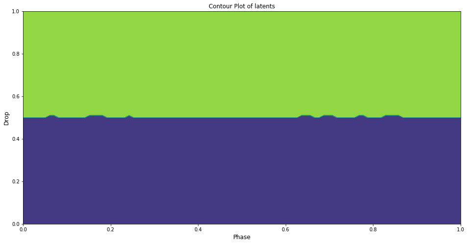
Figure 1: Contour plot for stationary sawbridge.

Fig 1 is a contour plot of the quantized latent as we vary the drop and phase parameter corresponding to variables $U$ and $V$ in (6). Note that the quantized latents are the quantized encoder outputs that are then fed to the decoder. Each of the two shaded regions of Fig 1 correspond to a single quantized latent vector that differ only in a single latent component. Since the regions correspond to whether the drop is greater than 0.5 or not, neural-network-based compressors trained using SGD converge to an optimal one-bit quantizer.

References

• [1] W. A. Pearlman and A. Said, Digital Signal Compression: Principles and Practice.   Cambridge University Press, 2011.
• [2] J. Ballé, P. A. Chou, D. Minnen, S. Singh, N. Johnston, E. Agustsson, S. J. Hwang, and G. Toderici, “Nonlinear transform coding,” IEEE Journal of Selected Topics in Signal Processing, vol. 15, no. 2, pp. 339–353, 2020.
• [3] A. B. Wagner and J. Ballé, “Neural networks optimally compress the sawbridge,” in 2021 Data Compression Conference (DCC), 2021, pp. 143–152.
• [4] P. Fleischer, “Sufficient conditions for achieving minimum distortion in a quantizer,” IEEE International Convention Record, vol. 12, no. 1, pp. 104–111, 1964.
• [5] A. Trushkin, “Sufficient conditions for uniqueness of a locally optimal quantizer for a class of convex error weighting functions,” IEEE Transactions on Information Theory, vol. 28, no. 2, pp. 187–198, 1982.
• [6] J. Kieffer, “Uniqueness of locally optimal quantizer for log-concave density and convex error weighting function,” IEEE Transactions on Information Theory, vol. 29, no. 1, pp. 42–47, 1983.
• [7] J. Max, “Quantizing for minimum distortion,” IRE Transactions on Information Theory, vol. 6, no. 1, pp. 7–12, 1960.
• [8] S. Lloyd, “Least squares quantization in PCM,” IEEE Transactions on Information Theory, vol. 28, no. 2, pp. 129–137, 1982.
• [9] A. Magnani, A. Ghosh, and R. M. Gray, “Optimal one-bit quantization,” in 2005 Data Compression Conference (DCC), 2005, pp. 270–278.
• [10] E. Abaya and G. Wise, “Some remarks on optimal quantization,” in Proc. Conf. on Inf. Sci. and Sys., Mar. 1982.
• [11] F. Wang, J. Fang, H. Li, Z. Chen, and S. Li, “One-bit quantization design and channel estimation for massive mimo systems,” IEEE Transactions on Vehicular Technology, vol. 67, no. 11, pp. 10 921–10 934, 2018.
• [12] J. Mo and R. W. Heath, “Capacity analysis of one-bit quantized mimo systems with transmitter channel state information,” IEEE Transactions on Signal Processing, vol. 63, no. 20, pp. 5498–5512, 2015.
• [13] S. Bhadane and A. B. Wagner, “On one-bit quantization,” to appear in arXiv.
• [14] E. Agustsson and L. Theis, “Universally quantized neural compression,” in Advances in Neural Information Processing Systems 33, 2020, pp. 12 367–12 376.