Sensitive Chandra coverage of a representative sample of weak-line quasars: revealing the full range of X-ray properties

Abstract

We present deeper Chandra observations for weak-line quasars (WLQs) in a representative sample that previously had limited X-ray constraints, and perform X-ray photometric analyses to reveal the full range of X-ray properties of WLQs. Only 5 of the 32 WLQs included in this representative sample remain X-ray undetected after these observations, and a stacking analysis shows that these 5 have an average X-ray weakness factor of $>85$. One of the WLQs in the sample that was known to have extreme X-ray variability, SDSS J1539+3954, exhibited dramatic X-ray variability again: it changed from an X-ray normal state to an X-ray weak state within $\approx$ 3 months in the rest frame. This short timescale for an X-ray flux variation by a factor of $\gtrsim 9$ further supports the thick disk and outflow (TDO) model proposed to explain the X-ray and multiwavelength properties of WLQs. The overall distribution of the X-ray-to-optical properties of WLQs suggests that the TDO has an average covering factor of the X-ray emitting region of $\sim$ 0.5, and the column density of the TDO can range from $N_{\rm H}$ $\sim 10^{23-24}~{}{\rm cm}^{-2}$ to $N_{\rm H}$ $\gtrsim 10^{24}~{}{\rm cm}^{-2}$, which leads to different levels of absorption and Compton reflection (and/or scattering) among WLQs.

1 Introduction

Investigations of the type 1 quasar sub-class of weak-line quasars (WLQs) have recently provided valuable insights into quasar structure and accretion physics. While WLQs are luminous blue quasars which are believed to be viewed generally face-on according to the standard unification model (e.g. Antonucci 1993; Netzer 2015), they have weak or no high-ionization emission lines (e.g. Fan et al., 1999; Diamond-Stanic et al., 2009; Plotkin et al., 2010; Wu et al., 2012), which marks how they differ from typical blue quasars. For example, their C iv rest-frame equivalent widths (REWs) are $\lesssim 10$–15 Å, corresponding to $\gtrsim 3\sigma$ negative deviations from the mean. Their C iv lines also often show very large blueshifts of 1000–10000 km s^-1. The majority of these WLQs are radio quiet.

X-ray studies of WLQs have proved particularly revealing for understanding their nature. A number of remarkable WLQ X-ray properties have been identified:

1. WLQs show a wide range of X-ray luminosities compared to expectations from their optical/UV luminosities or overall spectral energy distributions (SEDs), when considering, e.g. $\alpha_{\rm ox}$ and $\Delta\alpha_{\rm ox}$ (e.g. Wu et al. 2011, 2012; Luo et al. 2015; Ni et al. 2018). $\alpha_{\rm ox}$ is the slope of a nominal power law connecting the rest-frame 2500 Å and 2 keV monochromatic luminosities; i.e., $\alpha_{\rm ox}=0.3838\log(L_{\rm 2~{}keV}/L_{2500~{}\mathring{\rm{A}}})$ (e.g. Tananbaum et al. 1979; Strateva et al. 2005). $\alpha_{\rm ox}$ reflects the relative strength of a quasar’s X-ray emission to its UV emission, indicating a strong connection between the corona and the disk. This quantity is correlated with $L_{2500~{}\mathring{\rm{A}}}$. We also define $\Delta\alpha_{\rm ox}=\alpha_{\rm ox}({\rm Observed})-\alpha_{\rm ox}(L_{2500~{}\mathring{\rm{A}}})$, which quantifies the deviation of the observed X-ray luminosity relative to that expected from the $\alpha_{\rm ox}$-$L_{2500~{}\mathring{\rm{A}}}$ relation (e.g. Gallagher et al. 2006). $\Delta\alpha_{\rm ox}$ can thus serve as an indicator of a quasar’s X-ray emission strength compared to the expectation from its UV emission.

   About half of the WLQ population shows weak X-ray emission, often by notable factors of 10 or more; this fraction is much higher than present among the general quasar population (e.g. Pu et al., 2020; Timlin et al., 2020a). Typical blue quasars with weak X-ray emission are mostly broad absorption line (BAL) quasars with high levels of intrinsic X-ray absorption (e.g. Brandt et al. 2000; Gallagher et al. 2002, 2006; Fan et al. 2009), but the blue WLQs targeted in X-ray observations have been selected not to have BALs, mini-BALs, or other strong rest-frame UV absorption, which makes the high X-ray weak fraction among WLQs intriguing. However, owing to a high fraction of X-ray non-detections among X-ray weak WLQs, the X-ray weakness distribution remains poorly defined for large values of X-ray weakness. The other half of the WLQ population generally shows nominal-strength X-ray emission.

2. X-ray spectral analyses of the members of the WLQ population with nominal-strength X-ray emission, utilizing both individual-object and spectral-stacking approaches, show notably steep power-law spectra typically with photon indices of $\Gamma=2.1$–2.3 (Luo et al., 2015; Marlar et al., 2018). Among the general quasar population, such steep power-law spectra indicate accretion onto the supermassive black hole (SMBH) with high Eddington ratio ($L/L_{\rm Edd}$; e.g. Shemmer et al. 2008; Brightman et al. 2013), and thus it seems likely that WLQs generally have high $L/L_{\rm Edd}$. This conclusion is also supported by the C iv REWs and blueshifts of WLQs (e.g. Luo et al. 2015; Ni et al. 2018), as well as rough single-epoch estimates of $L/L_{\rm Edd}$ $\approx 0.3$–1.3 (e.g. Luo et al. 2015; Plotkin et al. 2015).

3. X-ray spectral analyses of the X-ray weak members of the WLQ population are more challenging, owing to limited numbers of detected counts in the available observations. Stacking analyses of the X-ray weak WLQs generally show hard X-ray spectra, on average, with effective power-law photon indices of $\langle\Gamma\rangle\approx 1.2$–1.4 (Luo et al., 2015; Ni et al., 2018). These hard X-ray spectra suggest high levels of intrinsic X-ray absorption ($N_{\rm H}\gtrsim 10^{23}$ cm^-2), which is somewhat surprising given these quasars’ type 1 nature and blue optical/UV continua without BAL (or other UV absoprtion) features. When such heavy X-ray absorption is present, Compton reflection and/or scattering may also play significant roles in shaping the X-ray spectrum. The presence of heavy X-ray absorption is further supported by an individual Chandra spectrum of SDSS J1521+5202, an extraordinarily luminous WLQ (Luo et al., 2015), and studies of some local WLQ analogs (e.g. Reeves et al. 2020).

4. The current limited multi-epoch X-ray observations of WLQs suggest that they show extreme large-amplitude X-ray variability events (e.g. Miniutti et al., 2012; Ni et al., 2020) more frequently than the general radio-quiet quasar population of comparable luminosity (e.g. Timlin et al., 2020b). The observed large-amplitude X-ray variability events are associated with changes between X-ray normal-strength and X-ray weak states, and they do not appear to have corresponding extreme optical/UV continuum or emission-line variations.

The above X-ray and multiwavelength results for WLQs have been used to construct a basic scenario that appears able to explain consistently their weak high-ionization lines, their X-ray properties, and some of their other multiwavelength properties (e.g. Lane et al., 2011; Wu et al., 2011, 2012; Luo et al., 2015; Ni et al., 2018). This scenario, depicted in Fig. 1 of Ni et al. (2018), proposes that, owing to high $L/L_{\rm Edd}$ ($\gtrsim 0.3$), WLQs have geometrically and optically thick inner accretion disks and associated outflows (e.g. Jiang et al., 2014, 2019; Wang et al., 2014; Dai et al., 2018). The thick disk and its outflow (hereafter, TDO), which lie near the central supermassive black hole, prevent ionizing EUV/X-ray photons from reaching much of the (substantially equatorial) high-ionization broad emission-line region (BLR), leading to the weak high-ionization lines. The TDO is also responsible for the X-ray weakness/absorption seen in about half of WLQs; X-ray weak WLQs arise for systems viewed at large inclinations, so that our line of sight intercepts the TDO. The large-amplitude X-ray variability events of some WLQs may arise from slight variations in the thickness of the TDO (e.g. rotation of an inner TDO that is somewhat azimuthally asymmetric) or internal motions of the TDO.

Our primary approach to investigating the X-ray properties of WLQs has involved Chandra “snapshot” (typically 2–5 ks) observations of luminous (typically $M_{i}\lesssim-27$), blue WLQs. While this approach has been successful for gaining a broad overview of basic WLQ X-ray properties, it has provided only limited insight into the X-ray properties of individual WLQs, especially for the most interesting X-ray weak members of this class. We know that many of these objects must be remarkably X-ray weak from X-ray stacking analyses, having $\Delta\alpha_{\rm ox}$ of $-0.4$ to $-0.7$, corresponding to X-ray weakness by factors of $\approx 11$–67 relative to a typical radio-quiet quasar. For comparison, our constraints on individual X-ray undetected objects typically can only show they have $\Delta\alpha_{\rm ox}\lesssim-0.3$, corresponding to X-ray weakness by a factor of $\gtrsim 6$. We thus currently lack useful information on the full distribution of $\Delta\alpha_{\rm ox}$ for WLQs, which should provide information about the nature of the TDO. Moreover, the limited individual-object X-ray constraints have hindered our ability to assess UV continuum and emission-line properties that may correlate with X-ray weakness, thereby serving as useful tracers of this behavior.

We have therefore performed additional, deeper (typically 5–23 ks) Chandra observations for a set of WLQs previously having limited X-ray constraints, and in this paper we present the observational results and their implications. With these observations, we now have complete, sensitive X-ray coverage for the well-defined sample of 32 WLQs with C iv REW $\lesssim 15$ Å defined by Ni et al. (2018). In addition to setting tighter X-ray constraints upon the properties of individual WLQs, these new observations add significantly to the number of WLQs with sensitive multi-epoch X-ray observations. They therefore also allow a search for additional examples of extreme large-amplitude X-ray variability events.

The layout of this paper is as follows. We describe the sample selection and Chandra observations in Section 2. In Section 3, we detail the X-ray photometric measurements and the derived X-ray-to-optical properties, and in Section 4 we briefly present relevant emission-line measurements. Section 5 presents our overall analysis results and discussion, and Section 6 presents a summary of our results. In Appendix A, we briefly present the results from new XMM-Newton observations of the extraordinarily luminous WLQ SDSS J1521+5202.

Throughout this paper, we use J2000 coordinates and a cosmology with $H_{0}=67.4$ km s^-1 Mpc^-1, $\Omega_{\rm M}=0.315$, and $\Omega_{\Lambda}=0.685$ (Planck Collaboration et al., 2020).

2 Sample selection and Chandra observations

In Ni et al. (2018), a sample of 32 WLQs with C iv REW $\lesssim$ 15 Å was constructed. These WLQs were selected from radio-quiet quasars in the SDSS Data Release 7 (DR7) quasar-properties catalog of Shen et al. (2011), including 10 of the most “extreme” (i.e. lowest C iv REW) WLQs with C iv REW $\lesssim$ 5 Å. They have $i$-band magnitude $m_{i}<$ 18.6 and a redshift satisfying $1.5<z<2.5$. As we want to avoid any potentially confusing X-ray absorption associated with, e.g. BAL winds, objects with BAL or mini-BAL features, narrow absorption features around C iv, or very red spectra with $\Delta(g-i)$ > 0.45 were excluded. Compared to other WLQ samples utilized in previous studies (e.g. Wu et al. 2011, 2012; Luo et al. 2015), this sample of WLQs has been selected in a relatively unbiased manner (no additional selection criteria such as high C iv blueshift and/or strong Fe ii/Fe iii emission were applied) and has a relatively large sample size. Thus, it can serve as a representative sample to study the WLQ population over the full range of C iv REW values seen among WLQs. WLQs in this representative sample have similar IR-to-UV SEDs (obtained from WISE, 2MASS, SDSS, and GALEX photometry) compared with typical quasars (see Luo et al. 2015; Ni et al. 2018 for details).

Among these 32 WLQs included in the representative sample of Ni et al. (2018), 12 WLQs were X-ray undetected (we note that these objects were only observed with 2–5 ks Chandra “snapshot” observations at that time; e.g. see Table 2 of Ni et al. 2018). Also, 2 WLQs need more secure X-ray measurements from Chandra; previously, their X-ray properties were adopted from the XMM-Newton slew-survey catalogue (Saxton et al., 2008) and the ROSAT all-sky survey catalogue (Boller et al., 2016) that have relatively large uncertainties compared to on-axis Chandra detections.

Chandra observations for these 14 WLQs were performed between 2019 December and 2020 August, using the Advanced CCD Imaging Spectrometer (Garmire et al., 2003) spectroscopic array (ACIS-S) with VF mode (which is also the mode adopted by the previous Chandra observations of these objects). For the 12 WLQs that were previously X-ray undetected, the exposure times were set to reach $\Delta\alpha_{\rm ox}$ upper limits of $\approx$ $-$0.5, if the objects remain X-ray undetected.

3 X-ray photometric measurements and X-ray-to optical properties

3.1 X-ray aperture-photometry analyses

Following the method described in Ni et al. (2018), we used Chandra Interactive Analysis of Observations (CIAO) tools (Fruscione et al., 2006) to process the new Chandra observations. We ran the CHANDRA_REPRO script to reprocess the observations, and then ran the DEFLARE script to remove background flares above a 3$\sigma$ level (see Table 1 for the flare-cleaned exposure times for each WLQ).

From the flare-cleaned event files, we produced images for each WLQ in the 0.5–8 keV (full), 0.5–2 keV (soft), and 2–8 keV (hard) bands with the standard ASCA grade set. In each band, we ran WAVDETECT on the image to detect sources with a false-positive probability threshold of 10^-6. If a source is detected in at least one band, we adopted the detected position closest to the SDSS position as the source position. If WAVDETECT does not detect any source within 1^′′ from the SDSS position, the SDSS position is adopted as the X-ray source position.

We performed aperture photometry in the soft band and the hard band for each observation. Source counts are extracted in the central 2^′′-radius region (which corresponds to an encircled-energy fraction of 0.959/0.907 in the soft/hard band for on-axis observations; e.g. Luo et al. 2015. Background counts are extracted from the annular region between the 10^′′-radius circle and the 40^′′-radius circle centered on the source position.

For each object in each band, we calculated a binomial no-source probability ($P_{B}$) from the source counts and background counts, which represents the probability of detecting the source counts by chance when no real source is present (e.g. Broos et al., 2007; Xue et al., 2011; Luo et al., 2015). For a certain band, when $P_{B}\leqslant 0.01$, the source is considered to be detected. We thus expect $<1$ false detection in our sample. The 1$\sigma$ errors of the source/background counts were obtained following Gehrels (1986) that is based on Poisson and binomial statistics. For sources considered to be undetected with $P_{B}>0.01$, the source counts upper limits at a 90% confidence level are derived following Kraft et al. (1991). We also calculated the band ratio (the ratio of hard-band counts to soft-band counts) and its uncertainty (or upper limit) utilizing the code BEHR (Park et al., 2006). From the band ratio, we derived the 0.5–8 keV effective power-law photon index ($\Gamma_{\rm eff}$) or its lower limit for each source with modelflux. The intrinsic X-ray photon spectra of quasars can typically be characterized by a power-law model, $N(E)\propto E^{-\Gamma}$, and $\Gamma_{\rm eff}$ derived here can serve as a good estimate of $\Gamma$ in the absence X-ray absorption; when X-ray absorption is present, $\Gamma_{\rm eff}$ provides a basic estimate of spectral hardening due to the absorption. The results are shown in Table 1. For sources that are undetected in both the soft and hard bands, we are unable constrain $\Gamma_{\rm eff}$. A nominal $\Gamma_{\rm eff}=1.4$ (which is the stacked $\Gamma_{\rm eff}$ of 30 X-ray weak WLQs in Luo et al. 2015) is assumed for these sources.

We also performed the above aperture-photometry analyses when stacking all archival Chandra observations available and the new Chandra observation together for each object. The stacked count rates are obtained with the CIAO command srcflux. Since WLQs may exhibit extreme X-ray variability (e.g. Ni et al., 2020), we first ensure that the count rates in all the epochs are consistent. As can be seen in Table 2, most of the WLQs do not show significant variations in count rate between the available Chandra epochs except for the object SDSS J153913.47+395423.4 (hereafter SDSS J1539+3954). SDSS J1539+3954 turned from an X-ray weak WLQ to an X-ray normal WLQ between 2013 and 2019, showing an extreme X-ray flux rise by a factor of $\gtrsim 20$ (Ni et al., 2020). According to our latest Chandra observation of this WLQ in 2020 June, it has now returned to being an X-ray weak WLQ (see Section 5.4). We perform stacked aperture-photometry analyses of this object utilizing only the two X-ray weak epochs.

3.2 X-ray to optical properties

We measured $\alpha_{\rm ox}$ values for the 12 WLQs that were previously Chandra undetected as well as the 2 WLQs that previously lacked high-quality Chandra detections. For previously X-ray undetected WLQs, the X-ray information utilized for calculating $\alpha_{\rm ox}$ is obtained from the stacked Chandra photometry (see Section 3.1).

The X-ray-to-optical power-law slope, $\alpha_{\rm ox}$, is defined as $0.3838\log(L_{\rm 2~{}keV}/L_{2500~{}\mathring{\rm{A}}})$, which is equal to $0.3838\log(f_{\rm 2~{}keV}/f_{2500~{}\mathring{\rm{A}}})$. In this formula, the observed flux density at rest-frame 2500 Å, $f_{\rm 2500~{}\mathring{\rm{A}}}$, is directly taken from the Shen et al. (2011) SDSS DR7 quasar-properties catalog. The Galactic-absorption corrected soft-band flux (which covers 2 keV in the rest frame for all our sources) is calculated from the net count rate in the soft band with srcflux to derive the 2 keV flux density, $f_{\rm 2~{}keV}$, assuming a power-law spectrum (with $\Gamma_{\rm eff}$ measured in Section 3.1) modified by Galactic absorption. If the source is undetected in the soft band, we calculate an upper limit for $f_{2{\rm keV}}$ following the same method from the upper limit on the soft-band net count rate. The $f_{\rm 2500~{}\mathring{\rm{A}}}$, $f_{\rm 2~{}keV}$, and calculated $\alpha_{\rm OX}$ values are all listed in Table 3.

We also derive the expected value of $\alpha_{\rm ox}$, $\alpha_{\rm OX}(L_{2500~{}\mathring{\rm{A}}})$, from the empirical $\alpha_{\rm OX}$–$L_{\rm 2500~{}{\textup{\AA}}}$ relation reported in Timlin et al. (2020a) for typical optically-selected quasars. We then calculate $\Delta\alpha_{\rm OX}$ from the observed $\alpha_{\rm ox}$ and the derived $\alpha_{\rm OX}(L_{2500~{}\mathring{\rm{A}}})$ to measure X-ray weakness relative to the expected X-ray luminosity (see Table 3).

With these updated X-ray-to-optical properties for 14 WLQs that were previously either X-ray undetected with loose X-ray upper limits or lacking high-quality Chandra detections, we have better constrained the X-ray-to-optical properties of the 32 WLQs in the Ni et al. (2018) WLQ representative sample. For the 12 WLQs that were previously X-ray undetected, 7 of them of are now X-ray detected as a result of the deeper observations. We note that the X-ray flux values of these detected objects are consistent with the flux upper limits previously obtained (see Table 2). For the five X-ray weak WLQs that still remain X-ray undetected (including SDSS J1539+3954, which has transitioned into an X-ray weak state; see Section 5.4 for details), we perform X-ray stacking analyses to assess their average properties, by adding the extracted source and background counts of these objects together. These X-ray stacking analyses (with 71.3 ks stacked exposure) show that the stacked source is still X-ray undetected, with $\Delta\alpha_{\rm ox}$ $<-0.74$, which corresponds to average X-ray weakness by a large factor of $>85$.

The distributions of $\alpha_{\rm OX}$ and $\Delta\alpha_{\rm OX}$ for this representative sample that consists of 32 objects are shown in Figures 1 and 2. We also compare the $\Delta\alpha_{\rm ox}$ distribution of WLQs with the $\Delta\alpha_{\rm ox}$ distribution of typical quasars from Appendix A of Timlin et al. (2020a) with the Anderson-Darling test. This Timlin et al. (2020a) “high X-ray detection fraction” quasar sample consists of 304 SDSS quasars (which are unobscured, broad-line AGNs) at $z=1.7$–2.7 with $i$-band magnitude $<$ 20.2 that have serendipitous sensitive Chandra X-ray observations (the detection fraction is $\approx 99.3\%$), with BAL and red quasars removed.

Since the Anderson-Darling test cannot properly utilize censored data, for 2 out of 304 quasars in the Timlin et al. (2020a) high-detection-fraction sample that only have $\Delta\alpha_{\rm ox}$ upper limits, their $\Delta\alpha_{\rm ox}$ values utilized in the analyses are drawn from the probability density function of the $\Delta\alpha_{\rm ox}$ values of other X-ray detected objects in the sample (the maximum value allowed to be drawn is set at the upper-limit value). For the 5 WLQs that are X-ray undetected, their $\Delta\alpha_{\rm ox}$ values are drawn from a normal distribution centered at their stacked $\Delta\alpha_{\rm ox}$ limit with a scatter of 0.1, with the maximum value allowed to be drawn as the upper-limit value. This procedure is repeated 1000 times to obtain an average test result, and this Monte Carlo approach is adopted throughout this work to account for the $\Delta\alpha_{\rm ox}$ upper limits of typical quasars/WLQs when performing statistical tests (see Section 5.2). We found that the $\Delta\alpha_{\rm ox}$ distributions of WLQs and typical quasars are different at a $\approx 4.5\sigma$ level. As we have already taken luminosity effects into account by converting $\alpha_{\rm ox}$ to $\Delta\alpha_{\rm ox}$, our comparison should be valid between samples with different luminosity ranges. We also note that this test result does not change materially when we limit our analyses to the bright objects in the Timlin et al. (2020a) high-detection-fraction sample with luminosities similar to those of WLQs in the representative sample. Among X-ray normal (or X-ray strong; $\Delta\alpha_{\rm OX}\geqslant-0.2$) objects, the $\Delta\alpha_{\rm ox}$ distributions of WLQs and typical quasars are not significantly different ($P_{\rm null}=0.26$). Among X-ray weak ($\Delta\alpha_{\rm OX}<-0.2$) objects, the $\Delta\alpha_{\rm ox}$ distributions of WLQs and typical quasars are different at a $\approx 2.9\sigma$ level. This indicates that WLQs differ from typical quasars mainly in having a strong tail toward X-ray weakness, as expected from the TDO model for WLQs.

We also use X-ray stacking analyses to derive the average spectral properties of X-ray weak WLQs and X-ray normal WLQs in the representative sample. The stacked $\Gamma_{\rm eff}$ is $1.1^{+0.2}_{-0.1}$ for X-ray weak WLQs, and $1.8^{+0.1}_{-0.1}$ for X-ray normal WLQs. These results further support the high apparent levels of intrinsic X-ray absorption, Compton reflection, and/or scattering among X-ray weak WLQs, supporting the existence of shielding materials with large column densities along our line sight, which we proposed to be the TDO (e.g. Luo et al. 2015; Ni et al. 2018).

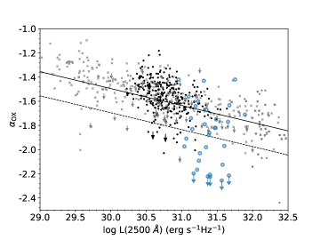
Figure 1: X-ray-to-optical power-law slope ($\alpha_{\rm ox}$) vs. $L_{\rm 2500~{}\mathring{\rm{A}}}$ for WLQs (blue symbols). In cases of X-ray non-detections, the 90% confidence upper limits of $\alpha_{\rm ox}$ are represented by the downward arrows. For comparison, the Timlin et al. (2020a) quasar sample that has a $\approx 99.3\%$ detection fraction (see Appendix A of Timlin et al. 2020a) is indicated by the black dots and downward arrows. Quasars from Steffen et al. (2006) and Just et al. (2007) are indicated by the gray crosses and downward arrows. The solid line shows the $\alpha_{\rm OX}$–$L_{\rm 2500~{}{\textup{\AA}}}$ relation from Timlin et al. (2020a); the dashed line ($\Delta\alpha_{\rm OX}=-0.2$) represents the adopted division between X-ray normal and X-ray weak quasars in this study, which corresponds to a $\approx 1.3\sigma$ ($\approx 90\%$ single-sided confidence level) offset given the $\Delta\alpha_{\rm ox}$ distribution (e.g. Steffen et al. 2006; Luo et al. 2015).

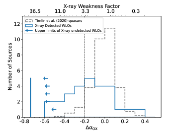
Figure 2: Distribution of $\Delta\alpha_{\rm OX}$ values. The solid histogram represents the $\Delta\alpha_{\rm ox}$ distribution of the 27 WLQs in the representative sample that are X-ray detected. The leftward arrows show the 90% confidence $\Delta\alpha_{\rm OX}$ upper limits for five X-ray non-detected WLQs. The vertical bar represents the stacked $\Delta\alpha_{\rm ox}$ upper limit for these X-ray non-detected WLQs. The dashed histogram represents the $\Delta\alpha_{\rm OX}$ distribution for the Timlin et al. (2020a) quasar sample that has a $\approx 99.3\%$ detection fraction, which is plotted for comparison (scaled to have the same apparent number of sources as the WLQ sample). The vertical dashed line (at $\Delta\alpha_{\rm OX}=-0.2$) represents the adopted threshold for defining X-ray weakness in this study.

4 Emission-line measurements

The C iv REWs of WLQs in the representative sample have been measured in Section 4.3 of Ni et al. (2018); C iv REW has been widely adopted to indicate the number of ionizing EUV photons reaching the high-ionization BLR. Since the strength of He ii $\lambda$1640 emission has also been shown to be an effective tracer of the number of EUV photons available (and it is a “cleaner” tracer compared to the C iv emission strength; e.g. Timlin et al. 2021 and references therein), we also measure the REWs of He ii emission for WLQs in the representative sample following the method of Timlin et al. (2021). The local continuum in the He ii emission region was obtained by fitting a linear model to the median values in the continuum windows 1420–1460 Å and 1680–1700 Å. The He ii REW was then measured by integrating directly the continuum-normalized flux in the window 1620–1650 Å. The errors of He ii REW are measured by perturbing the fluxes using the flux errors (see Timlin et al. 2021 for details). The median He ii REW error of WLQs in our sample is $\approx 0.6$ Å. If the He ii emission line is not detected significantly, an upper limit was estimated. The results can be seen in Table 4. We note that most of the WLQs do not have He ii emission detected; only upper limits for He ii REW are obtained. We also note that, as WLQs have weak and sometimes blueshifted high-ionization emission lines, there might be uncertainties associated with their redshift measurements. We verified that our He ii measurement results do not change materially when different redshift measurements are adopted (e.g. Hewett & Wild 2010; Schneider et al. 2010).

We also measure the He ii REW limits in the stacked spectrum of X-ray weak/normal WLQs in our sample. Each WLQ spectrum is normalized to its median flux value in the range 1700–1705 Å before being stacked together (see Timlin et al. 2021 for details about the stacking process). For the 16 X-ray weak WLQs in the representative sample, the stacked He ii REW upper limit is 0.12 Å. For the 16 X-ray normal WLQs, the stacked He ii REW upper limit is 0.29 Å.

5 Analysis results and discussion

5.1 Assessing and refining the TDO model for WLQs

The X-ray-to-optical properties of the representative WLQ sample as presented in Section 3.2 can give us some basic constraints on the nature of the TDO we proposed to explain the X-ray and multiwavelength properties of WLQs. From the $\Delta\alpha_{\rm ox}$ distribution of WLQs in our sample, we can infer that the TDO, if present, has an average global covering factor of $\approx 0.5$ among WLQs. The TDO should also be able to produce X-ray weakness by an average factor of $>85$ for $\approx 15\%$ of the WLQs, and by an average factor of $\approx$ 9 for $\approx 35\%$ of the WLQs, suggesting that the shielding column density could range from $N_{\rm H}$ $\sim 10^{23-24}~{}{\rm cm}^{-2}$ to $N_{\rm H}$ $\gtrsim 10^{24}~{}{\rm cm}^{-2}$. The X-ray weak WLQs in our sample have a stacked $\Gamma_{\rm eff}\approx 1.1$ and a stacked X-ray weakness factor of $\approx$ 13. To produce this level of X-ray weakness with a simple intrinsic absorption model, a TDO with $N_{\rm H}$ $\sim 5\times 10^{23}~{}{\rm cm}^{-2}$ is required. However, such a TDO will produce an X-ray spectrum with $\Gamma_{\rm eff}\sim 0.3$, which is not consistent with the stacked $\Gamma_{\rm eff}$ $\approx 1.1$ we obtained, suggesting that more complex absorption (and/or Compton reflection/scattering or a soft-excess component) is present, and that how the TDO modifies the X-ray properties varies from object-to-object. The complex absorption (and/or Compton-reflection/scattering) effects caused by the TDO are also indicated by the lack of bimodality in the $\Delta\alpha_{\rm ox}$ distribution of WLQs. If the TDO had a rather simple nature so that similar X-ray “blocking” effects were present among all X-ray weak WLQs, we should be able to observe a “clustering” of $\Delta\alpha_{\rm ox}$ on the X-ray weak side, rather than the long tail toward X-ray weakness observed in Figure 2.

We note that there are also other possible explanations for the distinctive X-ray properties of WLQs listed in Section 1, such as intrinsic differences/variations in the coronal emission, or gravitational light-bending that leads to different amounts of X-ray emission reaching the observer when the distances between the corona and the central black hole are different (e.g. Miniutti & Fabian 2004). However, neither of these scenarios can explain why the distinctive X-ray properties are only observed among WLQs rather than quasars with typical optical/UV emission-line properties – the link between these scenarios and weak emission lines is not clear. These scenarios also cannot explain the high apparent level of X-ray absorption we observed among X-ray weak WLQs.

Furthermore, while shielding materials located on a much larger (by a factor of $\gtrsim$ 100) scale might explain the X-ray properties of WLQs (e.g. “clumps” near the torus region), the cause for the defining weak high-ionization emission lines would remain unexplained. WLQs have IR-to-UV SEDs similar to those of typical quasars (e.g. Luo et al., 2015; Ni et al., 2018), so the weak high-ionization emission lines cannot be attributed to any obvious difference in the continuum level. As only shielding materials located between the central X-ray source and the high-ionization BLR can naturally explain all the multiwavelength properties of WLQs, the TDO model (which includes both a thick disk and an outflow component) seems to be the most viable available solution.

5.2 $\Delta\alpha_{\rm ox}$-C iv REW and $\Delta\alpha_{\rm ox}$-He ii REW distributions of WLQs vs. typical quasars

The relations between $\Delta\alpha_{\rm ox}$ and C iv REW or He ii REW among typical quasars reflect the link between the X-ray emission strength and the strength of the ionizing EUV continuum (e.g. Timlin et al. 2021 and references therein). While EUV photons may be generated from a “warm corona" in the inner-disk region via Comptonization (e.g. Petrucci et al. 2018) and X-ray photons are thought to be produced by the “hot corona” in the vicinity of the central black hole, these relations indicate that there is a strong coupling between the X-ray emission and EUV emission. The unusual X-ray properties of WLQs and their weak emission lines naturally lead one to wonder whether the relation between $\Delta\alpha_{\rm ox}$ and C iv or He ii REW also applies to WLQs, and whether this may challenge the universal existence of the coupling between the X-ray emission and the EUV emission among quasars.

In the $\Delta\alpha_{\rm ox}$ vs. log C iv REW space, WLQs appear to show relatively larger scatter compared to typical quasars in Timlin et al. (2020a) (see the left panel of Figure 3). To test whether the deviations of WLQs from the $\Delta\alpha_{\rm ox}$-C iv REW relation are statistically different compared to those of typical quasars, we use the Anderson-Darling test with the Monte Carlo procedure as described in Section 3.2. All 32 WLQs and 637 quasars in the Timlin et al. (2020a) sample that have C iv detections are utilized in the Anderson-Darling test, including 5 WLQs and 18 quasars in the Timlin et al. (2020a) sample that only have $\Delta\alpha_{\rm ox}$ upper limits.

We found that the difference in the distributions of $\Delta\alpha_{\rm ox}$ residuals from the best-fit $\Delta\alpha_{\rm ox}$-log C iv REW relation reported in Timlin et al. (2020a) (as can be seen in the left panel of Figure 3) among WLQs and typical quasars is significant at a $\approx 4.0~{}\sigma$ level.

To test whether the observed phenomenon is influenced by the Baldwin effect (which shows that C iv REW is strongly linked with $L_{\rm 2500~{}\mathring{\rm{A}}}$; e.g. Baldwin 1977), we perform the above analyses for $\Delta\alpha_{\rm ox}$ and $\Delta$log C iv REW (which is calculated as log C iv REW minus the expected log C iv REW value from the C iv REW-$L_{\rm 2500~{}\mathring{\rm{A}}}$ relation reported in Timlin et al. 2020a). The best-fit $\Delta\alpha_{\rm ox}$-$\Delta$log C iv REW relation is derived utilizing the Python package linmix (Kelly, 2007). We found that the difference in the distributions of $\Delta\alpha_{\rm ox}$ residuals from the $\Delta\alpha_{\rm ox}$-$\Delta$log C iv REW relation (as can be seen in the right panel of Figure 3) between WLQs and typical quasars is still significant at a $\approx 4.0~{}\sigma$ level according to the Anderson-Darling test. The above analysis results do not change qualitatively when we limit our comparisons to WLQs and the brightest 64 objects among the Timlin et al. (2020a) quasars with C iv detections, which have similar luminosities to the WLQs in our representative sample and are all X-ray detected. The above analysis results also do not change qualitatively when we perturb the $\Delta\alpha_{\rm ox}$ values with the measurement errors.

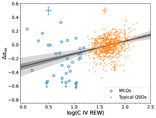
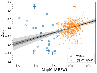
Figure 3: Left: $\Delta\alpha_{\rm ox}$ vs. log C iv REW (in units of Å) for WLQs in the representative sample as well as typical quasars in Timlin et al. (2020a). Right: $\Delta\alpha_{\rm ox}$ vs. $\Delta$log C iv REW for WLQs in the representative sample as well as typical quasars in Timlin et al. (2020a). The best-fit $\Delta\alpha_{\rm ox}$-C iv REW ($\Delta\alpha_{\rm ox}$-$\Delta$log C iv REW) relation (Timlin et al., 2020a) is shown as the black solid line, with its 1$\sigma$/3$\sigma$ confidence intervals shown as the dark/light gray-shaded region in the left (right) panel. The median measurement errors of $\Delta\alpha_{\rm ox}$ and C iv REW for WLQs and typical quasars are shown as error bars at the top of each panel.

We also use the Peto-Prentice test with a Monte Carlo approach to assess if the deviations of WLQs and typical quasars from the $\Delta\alpha_{\rm ox}$-He ii REW relation derived in Timlin et al. (2021) are different (see the left panel of Figure 4); the Peto-Prentice test can incorporate the censored measurements of He ii into the analyses. For 5 WLQs and 21 out of 206 quasars in the Timlin et al. (2021) sample that only have $\Delta\alpha_{\rm ox}$ upper limits, their $\Delta\alpha_{\rm ox}$ values utilized in the analysis are drawn following the method described in Section 3.2. We can see that in the $\Delta\alpha_{\rm ox}$ vs. log He ii REW space, WLQs exhibit obviously larger scatter compared to typical quasars. We found that the difference in the distributions of residuals from the $\Delta\alpha_{\rm ox}$-He ii REW relation between WLQs and typical quasars is significant at $\approx 5.6\sigma$ according to the Peto-Prentice test.

It has also been found that for typical quasars, $\Delta\alpha_{\rm ox}$ follows a tight correlation with the difference between log values of measured He ii REWs and expected He ii REWs from the He ii REW-$L_{\rm 2500~{}\mathring{\rm{A}}}$ relation ($\Delta$log He ii REW; Timlin et al. 2021), as shown by the black line in the right panel of Figure 4. However, WLQs in our representative sample do not follow this relation in a similar pattern as that of typical quasars, again showing larger scatter. We also use the Peto-Prentice test to assess statistically the difference in the residuals of $\Delta\alpha_{\rm ox}$ values compared to the expectation from the $\Delta\alpha_{\rm ox}$-$\Delta$log He ii REW relation between WLQs and typical quasars. We found that this difference is significant at $\approx 7.8\sigma$. The above analysis results do not change qualitatively when we limit our comparisons to WLQs and the brightest 64 objects among the Timlin et al. (2021) quasars, which have similar luminosities to the WLQs in our representative sample with an X-ray detection fraction of $\approx 92\%$. The above analysis results also do not change qualitatively when we perturb the $\Delta\alpha_{\rm ox}$ values with the measurement errors.

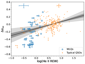
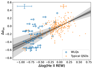
Figure 4: Left: $\Delta\alpha_{\rm ox}$ vs. log He ii REW (in units of Å) for WLQs in the representative sample as well as typical quasars in Timlin et al. (2021). Right: $\Delta\alpha_{\rm ox}$ vs. $\Delta$log He ii REW for WLQs in the representative sample as well as typical quasars in Timlin et al. (2021). The best-fit $\Delta\alpha_{\rm ox}$-He ii REW ($\Delta\alpha_{\rm ox}$-$\Delta$log He ii REW) relation reported in Timlin et al. (2021) is shown as the black solid line, with its 1$\sigma$/3$\sigma$ confidence intervals shown as the dark/light gray-shaded region in the left (right) panel. The median measurement errors of $\Delta\alpha_{\rm ox}$ and He ii REW for WLQs and typical quasars are shown as error bars at the top of each panel.

The statistical test results above clearly indicate that, in the $\Delta\alpha_{\rm ox}$ vs. high-ionization emission-line strength space, WLQs do not behave in a manner similar to that of typical quasars (WLQs have larger scatter). However, this does not necessarily mean that the link between X-ray emission and EUV emission that exists among the general quasar population is not applicable to WLQs, as C iv REW or He ii REW can only serve as an indicator of the number of EUV photons that reach the high-ionization BLR (where the relevant emission lines are produced) rather than the total number of EUV photons emitted, and $\Delta\alpha_{\rm ox}$ can only measure the relative strength of the X-ray emission that has successfully reached the observer.

The TDO model is plausibly able to explain why the distribution of WLQs’ deviations from the $\Delta\alpha_{\rm ox}$-C iv (or He ii) REW relation is broader than that of typical quasars, while the coupling between intrinsic X-ray emission and EUV emission still holds. In the context of the TDO model, the ionizing EUV photons produced are largely prevented from reaching the BLR due to shielding by the TDO (e.g. see Figure 1 of Ni et al. 2018). For X-ray normal WLQs, if their EUV emission were not heavily shielded by the TDO, their C iv/He ii REWs should not be as small as observed. According to the correlation between $\Delta\alpha_{\rm ox}$ and C iv (or He ii) REW, we expect them to have $\Delta\alpha_{\rm ox}$ values similar to those of typical quasars, which is consistent with their observed X-ray emission strength (see Section 3.2). For X-ray weak WLQs, not only is their EUV emission strength not represented by their C iv/He ii REWs, but also their $\Delta\alpha_{\rm ox}$ values cannot serve as measurements of the intrinsic X-ray emission strength. The $\Delta\alpha_{\rm ox}$ values of X-ray weak WLQs reflect the observed X-ray emission strength with the presence of the TDO along the line of sight, which blocks the intrinsic X-ray emission with heavy absorption. Thus, these X-ray weak WLQs fall below the $\Delta\alpha_{\rm ox}$-C iv REW (or He ii REW) relation when we “relocate” them to have C iv/He ii REWs similar to those of typical quasars. When we consider the WLQ population altogether, the significantly larger scatter of WLQs compared to that of typical quasars in Figures 3 and 4 is expected, as the X-ray weak WLQs are “moved” downward along the $\Delta\alpha_{\rm ox}$ axis by the TDO. The larger scatters of WLQs compared to typical quasars in the $\Delta\alpha_{\rm ox}$ vs. C iv (or He ii) REW space lead to the significant test results when comparing the deviations of these two samples from the best-fit relation. As the He ii REW serves as a better tracer of EUV ionizing photons (e.g. see Timlin et al. 2021 and references therein), typical quasars have a smaller scatter in the $\Delta\alpha_{\rm ox}$ vs. He ii REW space compared to the $\Delta\alpha_{\rm ox}$ vs. C iv REW space. Thus, the test results are more significant in the $\Delta\alpha_{\rm ox}$ vs. He ii REW space.

5.3 Spectral tracers of X-ray weakness among WLQs

In Ni et al. (2018), we identified $\Delta(g-i)$ and Fe ii REW as potential tracers of X-ray weakness among WLQs. With 7 additional X-ray detections and the improved $\Delta\alpha_{\rm ox}$ constraints for objects that remain X-ray undetected, these conclusions still hold, with test statistics roughly unchanged compared to Ni et al. (2018). The significance levels of the correlations between $\Delta\alpha_{\rm ox}$ and $\Delta(g-i)$ or Fe ii REW are close to, but below, 3$\sigma$ for the WLQ representative sample. The details are shown in Figures 5 and 6. Both relations have considerable scatter. We also note that the combination of $\Delta(g-i)$ and Fe ii is not able to give a significantly better prediction of $\Delta\alpha_{\rm ox}$ than either of these quantities individually.

We note that for the Full sample in Ni et al. (2018) that has 63 WLQs, both $\Delta(g-i)$ and Fe ii REW correlate with $\Delta\alpha_{\rm ox}$ significantly. However, around half of the objects in the Full sample were not selected in an unbiased manner; they were selected for Chandra observations with additional requirements such as large C iv blueshifts and strong Fe ii/Fe iii emission. Thus, while both $\Delta(g-i)$ and Fe ii REW have the potential to predict X-ray weakness, we still need a larger sample of WLQs that have been selected in an unbiased manner to confirm it. This will help to clarify the nature of the shielding material among WLQs, which we propose to be the TDO. In the context of the TDO model, whether a WLQ is observed as X-ray weak or X-ray normal is largely determined by its inclination angle. If the relation between $\Delta\alpha_{\rm ox}$ and $\Delta(g-i)$ is confirmed, it might be explained if the amount of dust tends to increase toward the equatorial plane (e.g. see Elvis 2012; Luo et al. 2015 for details). This would cause mild excess reddening when quasars are viewed at large inclination angles, so that X-ray weak WLQs have redder colors compared to those of X-ray normal WLQs. If the relation between $\Delta\alpha_{\rm ox}$ and Fe ii REW is confirmed, it may be a consequence of aspect-dependent effects of the disk emission (e.g. Wang et al. 2014).

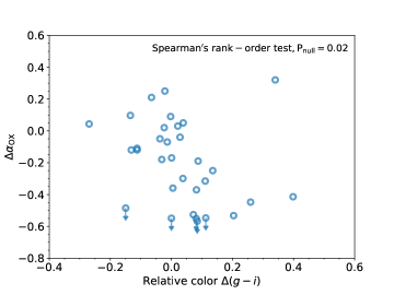
Figure 5: $\Delta\alpha_{\rm ox}$ vs. relative color for WLQs in the representative sample. For X-ray non-detections, the 90% confidence upper limits of $\Delta\alpha_{\rm OX}$ are marked as the downward arrows.

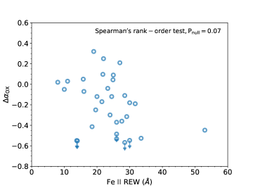
Figure 6: $\Delta\alpha_{\rm ox}$ vs. Fe ii REW for WLQs in the representative sample. For X-ray non-detections, the 90% confidence upper limits of $\Delta\alpha_{\rm OX}$ are marked as the downward arrows.

5.4 X-ray variability of WLQs

Among 12 WLQs in our sample that have been observed by Chandra at least twice, SDSS J1539+3954 is the only WLQ that has so far shown extreme X-ray variability. Particularly, it has experienced two extreme X-ray state changes within 7 years (see Figure 7). We note that the 2020 Chandra observation of SDSS J1539+3954 was taken with Chandra Director’s Discretionary Time, aiming to investigate further the X-ray variability of this object. We did observe an extreme X-ray flux change again within nine months (which is $\approx 3$ months in the rest frame); specifically, the flux dropped by a factor of $\gtrsim 9$ between 2019 September and 2020 June to return this quasar to an X-ray weak level. As stated in Ni et al. (2020), the Hobby-Eberly Telescope (HET) observation taken contemporaneously with the 2019 September Chandra observation shows that the UV continuum level of this object remains generally unchanged despite the dramatic increase in the X-ray flux, and its emission lines remain weak. Our new HET observation in 2020 June taken contemporaneously with the latest Chandra observation further confirms this (see Figure 8), considering the $\approx 20\%$ uncertainty of HET flux calibration. The photometric data collected by the Zwicky Transient Facility (ZTF; Bellm et al. 2019), displayed in Figure 9, also show the variation of the $g$/$r$-band magnitude of SDSS J1539+3954 between 2018 and 2021 (when compared to the median magnitude value in this time range) is $\lesssim 0.2/0.1$ mag, consistent with the expectations for typical quasars (e.g. see figure 3 of MacLeod et al. 2012).

This extreme X-ray variability of SDSS J1539+3954 could be explained in the context of the TDO model. We naturally expect the transition between an X-ray weak state and an X-ray normal state when there is a slight change in the thickness of the TDO that moved across our line of sight, and the observed UV continuum/emission-line properties will not be significantly affected. While a significant change in the global TDO structure could take up to years, if the extreme X-ray variability is caused by slight variations in the height of the TDO, such as due to the rotation of an azimuthally asymmetric TDO, the timescale of an X-ray state transition could be small (e.g., weeks-to-months in the rest frame), which could explain the small timescale ($\approx 3$ months) of the X-ray state transition we recently observed for SDSS J1539+3954.

In Ni et al. (2020), we noted that the extreme X-ray variability of SDSS J1539+3954 is reminiscent of that previously found for another WLQ, PHL 1092 at $z=0.39$, which showed a flux dimming and then re-brightening by a factor of $\approx 260$ during 2003–2010 (e.g. Miniutti et al. 2012). This similarity suggests that weak UV emission lines may be an effective indicator for finding extreme X-ray variability among luminous quasars, especially when considering the limited X-ray monitoring performed thus far for WLQs. Moreover, the $z=0.18$ quasar PDS 456 has similar C iv properties to WLQs (e.g. O’Brien et al. 2005) and shows notably large-amplitude X-ray variability (e.g. Reeves et al. 2020 and references therein), further strengthening the likely connection. Additional X-ray monitoring of WLQs is thus warranted. We also note that local Narrow-Line Seyfert 1 galaxies (NLS1s), generally thought to have high Eddington ratios, have been proposed to follow a physical model with broad similarities to our TDO scenario for WLQs (e.g. Done & Jin 2016; Hagino et al. 2016) and that some NLS1s show extraordinary X-ray variability (e.g. Boller et al. 1997; Boller et al. 2021; Leighly 1999; Parker et al. 2021). Some of this X-ray variability may also be caused by motions of a TDO across the line of sight.

In addition to confirming the link between weak UV emission lines and extreme X-ray variability to support the TDO model, X-ray monitoring of WLQs can also help reveal whether the TDO wind varies dramatically itself (e.g. via the motions of internal clumps), and is able to cause X-ray state transitions as well. If a large fraction of WLQs exhibit extreme variability during long-term X-ray monitoring, it would suggest that their X-ray state transitions are not purely the results of slight changes in the height of a TDO that moved across our line of sight, as we should only observe such extreme X-ray variability events among WLQs where our line of slight roughly skims the “surface” of the TDO according to the model. Alternatively, if only a small fraction (though this fraction should still be considerably larger compared to that among typical quasars) of WLQs show extreme X-ray variability, it would suggest that the internal motion of the TDO is unlikely to be strong enough to lead to X-ray state transitions. Currently, multi-epoch ($\approx 2$) Chandra observations have been obtained for 12 WLQs in our sample, and SDSS J1539+3954 is the only one showing extreme X-ray variability. We will be able to obtain more information after further monitoring these WLQs.

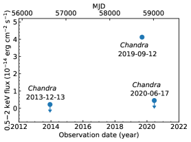
Figure 7: The historical 0.5–2 keV X-ray flux of SDSS J1539+3954. The solid circle represents the detected flux; downward arrows represent the upper limits on flux obtained from a non-detection. This quasar rose in X-ray flux by a factor of $\gtrsim 20$ (Ni et al., 2020) and then declined by a factor of $\gtrsim 9$.

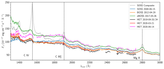
Figure 8: Spectra of SDSS J1539+3954 taken at different epochs. For HET spectra, we mask the areas suffering from channel discontinuities and telluric absorption (G. Zeimann 2019, private communication). The SDSS quasar composite spectrum from Vanden Berk et al. (2001) is scaled to the 2004 SDSS spectrum of SDSS J1539+3954 at rest-frame 2240 Å and plotted in the background for comparison. Note that the emission lines (e.g. C iv) remained weak despite the strong X-ray flux variations occurring contemporaneously.

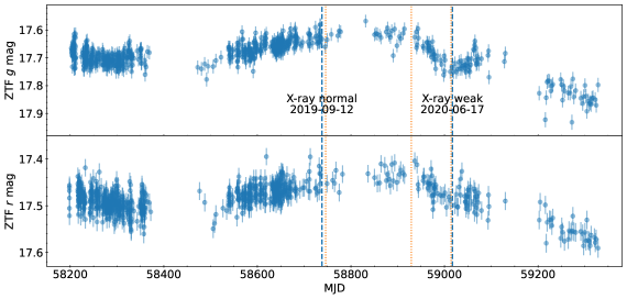
Figure 9: The $g$/$r$-band lightcurves of SDSS J1539+3954 from ZTF. The blue dashed lines mark the dates of the Chandra observations, and the orange dotted lines mark the dates of the HET observations. Note that the observed variation in the $g$/$r$-band magnitude between the X-ray normal state and the X-ray weak state is typical among luminous quasars.

6 Conclusions and Future Work

In this work, we present the observational results for a set of WLQs in a representative WLQ sample that only had limited X-ray constraints previously, and perform statistical analyses to study this representative sample. The key points are listed below:

1. We observed 12 X-ray undetected WLQs in the Ni et al. (2018) representative sample with deeper Chandra observations, and detected 7 of these WLQs. We also re-observed 2 WLQs in the Ni et al. (2018) sample with Chandra that required more secure X-ray data (see Section 2).

2. We performed photometric analyses to estimate the X-ray fluxes of the WLQs with new Chandra observations (see Section 3.1). For WLQs that are still undetected, tight X-ray flux upper limits are obtained. For one of the WLQs in our sample, SDSS J1539+3954, we found that after an observed X-ray flux rise by a factor of $\gtrsim 20$ reported in Ni et al. (2020), it changed from an X-ray normal state back to an X-ray weak state within $\approx$ 3 months in the rest frame, with a downward variation in the X-ray flux by a factor of $\gtrsim$ 9. The TDO model proposed for WLQs can explain these dramatic X-ray flux variations (see Section 5.4).

3. We updated the X-ray-to-optical properties of the Ni et al. (2018) representative WLQ sample, and compared the $\Delta\alpha_{\rm ox}$ distribution of this WLQ sample with that of typical quasars. We found that the $\Delta\alpha_{\rm ox}$ values of WLQs differ from those of typical quasars significantly, mainly because of a strong tail toward X-ray weakness. X-ray stacking analyses show that for 5 out of 32 WLQs that are still X-ray undetected, they are X-ray weak by an average factor of $>85$ (see Section 3.2).

4. The $\Delta\alpha_{\rm ox}$ distribution of WLQs in our representative sample suggests that the TDO, if responsible for the X-ray properties of WLQs, has an average global covering factor of $\sim$ 0.5. The column density of the TDO among different objects may range from $N_{\rm H}$ $\sim 10^{23-24}~{}{\rm cm}^{-2}$ to $N_{\rm H}$ $\gtrsim 10^{24}~{}{\rm cm}^{-2}$, causing different levels of absorption and Compton reflection (and/or scattering). This is also broadly supported by the non-bimodal nature of the $\Delta\alpha_{\rm ox}$ distribution (see Section 5.1).

5. We found that the scatter of WLQs around the $\Delta\alpha_{\rm ox}$ vs. C iv REW and the $\Delta\alpha_{\rm ox}$ vs. He ii REW relations for typical quasars are significantly larger than those of typical quasars. The differences are consistent with expectations from the TDO model (see Section 5.2).

6. We found that after obtaining a better characterization of the X-ray-to-optical properties of the Ni et al. (2018) representative WLQ sample, the significance levels of the correlations between $\Delta\alpha_{\rm ox}$ and $\Delta(g-i)$ or Fe ii REW (which are regarded as potential tracers of X-ray weakness among WLQs) are still below $3\sigma$ (see Section 5.3).

   In the future, a larger sample of WLQs with X-ray detections that are selected in an unbiased manner will help us to investigate further the potential tracers of X-ray weakness, which will ultimately enable us to probe the nature of WLQs and test the TDO model. Long-term X-ray monitoring of a sample of WLQs as well as X-ray spectral observations of SDSS J1539+3954 will also enable us to examine further the TDO model, as the TDO model predicts a certain fraction of WLQs with extreme X-ray variability (this fraction is expected to be considerably larger compared to that among typical quasars) and a high apparent level of absorption in the X-ray weak state of SDSS J1539+3954. Comparisons between WLQs and other objects known to have high Eddington ratios such as NLS1s will also help to reveal the underlying physics of these objects.

DATA AVAILABILITY

The data used in this investigation are available in the article.

Table 1: New X-ray Observations and Photometric Properties of WLQs

Object Name	RA	Dec	Redshift	Observation	Observation	Exposure	Soft Band	Hard Band	Band	$\Gamma_{\rm eff}$	Ref.
(J2000)	(deg)	(deg)		ID	Start Date	Time (ks)	(0.5–2 keV)	(2–8 keV)	Ratio
(1)	(2)	(3)	(4)	(5)	(6)	(7)	(8)	(9)	(10)	(11)	(12)
Previously X-ray undetected objects in the representative sample
$082508.75+115536.3$	126.286476	11.926766	1.992	22527	2020-09-29	6.6	$<4.0$	$<2.5$	…	…	Luo et al. (2015)
$082722.73+032755.9$	126.844727	3.465551	2.031	22533	2019-09-30	10.1	$3.0^{+3.1}_{-1.7}$	$<5.9$	$<2.37$	> 0.4	Luo et al. (2015)
				22865	2019-10-01	10.0	$2.0^{+2.8}_{-1.3}$	$<5.9$	$<3.89$	> 0.1	Luo et al. (2015)
$094533.98+100950.1$	146.391617	10.163917	1.672	22529	2019-10-27	12.0	$4.1^{+3.3}_{-2.0}$	$5.3^{+3.7}_{-2.4}$	$1.3^{+1.4}_{-0.9}$	$0.9^{+0.8}_{-0.6}$	Wu et al. (2012)
$095023.19+024651.7$	147.596664	2.781048	1.882	22532	2020-01-25	15.7	< 5.6	< 5.9	…	…	Ni et al. (2018)
$100517.54+331202.8$	151.323105	33.200783	1.802	22535	2020-01-17	23.3	$13.3^{+4.9}_{-3.7}$	$9.4^{+4.5}_{-3.2}$	$0.8^{+0.5}_{-0.3}$	$1.2^{+0.3}_{-0.4}$	Luo et al. (2015)
$110409.96+434507.0$	166.041519	43.751972	1.804	22708	2020-02-10	15.1	< 2.4	$2.9^{+3.2}_{-1.8}$	> 2.80	< 0.3	Ni et al. (2018)
$122311.28+124153.9$	185.797028	12.698329	2.068	22709	2020-03-22	15.6	$10.3^{+4.5}_{-3.2}$	$8.4^{+4.4}_{-3.0}$	$0.8^{+0.6}_{-0.4}$	$1.2^{+0.5}_{-0.4}$	Ni et al. (2018)
$122855.90+341436.9$	187.232941	34.243595	2.147	22530	2020-02-26	14.7	$4.1^{+3.3}_{-2.0}$	$<5.9$	$<1.74$	> 0.6	Ni et al. (2018)
$134601.28+585820.2$	206.505341	58.972279	1.664	22531	2020-04-09	12.4	< 2.4	< 4.2	…	…	Luo et al. (2015)
$140710.26+241853.6$	211.792786	24.314896	1.668	22534	2020-08-23	17.5	$7.1^{+3.9}_{-2.7}$	$4.0^{+3.5}_{-2.1}$	$0.6^{+0.6}_{-0.4}$	$1.5^{+0.7}_{-0.5}$	Luo et al. (2015)
$153913.47+395423.4$	234.806137	39.906513	1.930	23132	2020-06-17	5.0	< 2.4	< 2.5	…	…	Luo et al. (2015); Ni et al. (2020)
$163810.07+115103.9$	249.541992	11.851092	1.983	22710	2020-01-04	13.1	< 2.4	< 4.2	…	…	Ni et al. (2018)
Objects in the representative sample that previously lacked Chandra observations
$113949.39+460012.9$	174.955795	46.003604	1.859	22712	2020-07-22	4.5	$16.7^{+5.3}_{-4.1}$	$7.6^{+4.2}_{-2.8}$	$0.5^{+0.3}_{-0.2}$	$1.6^{+0.3}_{-0.4}$	Ni et al. (2018)
$123326.03+451223.0$	188.358459	45.206402	1.966	22711	2020-08-15	2.7	$25.0^{+6.2}_{-5.1}$	$18.7^{+5.7}_{-4.5}$	$0.7^{+0.3}_{-0.2}$	$1.2^{+0.3}_{-0.2}$	Ni et al. (2018)

Note. — Col. (1): Object name in the J2000 coordinate format. Cols. (2)–(3): The SDSS position in decimal degrees. Col. (4): Redshift adopted from Hewett & Wild (2010). Cols. (5)–(6): The ID and start date of the Chandra observations. Col. (7): Effective exposure time in the full band (0.5–8 keV) with background flares cleaned. Cols. (8)–(9): Source counts (aperture-corrected) in the soft band (0.5–2 keV) and hard band (2–8 keV). If the source is undetected in a band, an upper limit of counts at a 90% confidence level is listed. Col. (10): Ratio of the hard-band and soft-band counts. “…” indicates that the source is not detected in both bands. Col. (11): Effective power-law photon index in the 0.5–8 keV band. “…” indicates that $\Gamma_{\rm eff}$ cannot be constrained. Col. (12): Reference paper for the object where its previous Chandra observations are presented.

Table 2: Stacked X-ray Photometric Properties of Previously X-ray Undetected WLQs

Object Name	Observation	Single-epoch Count	Total Exposure	Stacked Soft Band	Stacked Hard Band	Band	$\Gamma_{\rm eff}$	Ref.
(J2000)	IDs	Rate (0.5–2 keV)	Time (ks)	(0.5–2 keV) Counts	(2–8 keV) Counts	Ratio
(1)	(2)	(3)	(4)	(5)	(6)	(7)	(8)	(9)
$082508.75+115536.3$	14951, 22527	$<0.47$, $<0.60$	11.7	$<4.0$	$<2.5$	…	…	Luo et al. (2015)
$082722.73+032755.9$	15342, 22533, 22865	$<0.97$, 0.30, 0.20	22.5	$5.1^{+2.7}_{-2.1}$	$3.8^{+2.5}_{-1.8}$	$0.7^{+0.6}_{-0.5}$	$1.3^{+0.7}_{-0.5}$	Luo et al. (2015)
$094533.98+100950.1$	12706, 22529	$<1.04$, 0.45	12.0	$4.1^{+2.6}_{-1.8}$	$5.1^{+2.8}_{-2.1}$	$1.2^{+1.0}_{-0.7}$	$0.9^{+0.7}_{-0.4}$	Wu et al. (2012)
$095023.19+024651.7$	18118, 22532	$<0.85$, $<0.36$	20.5	$3.0^{+2.3}_{-1.5}$	< 7.6	$<3.2$	$>0.2$	Ni et al. (2018)
$100517.54+331202.8$	15351, 22535	$<1.38$, 0.60	23.3	$13.6^{+4.2}_{-3.5}$	$9.1^{+3.6}_{-2.9}$	$0.7^{+0.3}_{-0.3}$	$1.3^{+0.4}_{-0.3}$	Luo et al. (2015)
$110409.96+434507.0$	18119, 22708	$<0.53$, $<0.16$	19.7	$<2.4$	< 7.6	…	…	Ni et al. (2018)
$122311.28+124153.9$	18115, 22709	$<0.89$, 0.66	20.1	$11.5^{+3.9}_{-3.2}$	$9.1^{+3.6}_{-2.9}$	$0.8^{+0.4}_{-0.3}$	$1.2^{+0.4}_{-0.3}$	Ni et al. (2018)
$122855.90+341436.9$	18111, 22530	$<1.05$, 0.37	14.7	$5.0^{+2.7}_{-2.0}$	< 5.9	< 1.4	> 0.8	Ni et al. (2018)
$134601.28+585820.2$	15336, 22531	$<1.57$, $<0.22$	12.4	< 2.4	< 4.2	…	…	Luo et al. (2015)
$140710.26+241853.6$	15345, 22534	$<0.97$, 0.41	20.0	$7.3^{+3.2}_{-2.5}$	$3.8^{+2.6}_{-1.8}$	$0.5^{+0.4}_{-0.3}$	$1.5^{+0.7}_{-0.4}$	Luo et al. (2015)
$153913.47+395423.4^{*}$	14948, 22528, 23132	$<0.45$, 3.98,$<0.48$	10.3	< 2.4	< 2.5	…	…	Luo et al. (2015); Ni et al. (2020)
$163810.07+115103.9$	18116, 22710	$<0.59$, $<0.18$	17.2	< 2.4	< 4.2	…	…	Ni et al. (2018)

Note. — Col. (1): Object name in the J2000 coordinate format. Col. (2): The IDs of all Chandra observations of this object. Col. (3): The 0.5–2 keV Chandra count rate in each Chandra observation. Col. (4): Total effective exposure time in the full band (0.5–8 keV) with background flares cleaned of all the available Chandra observations. Cols. (5)–(6): Stacked source counts (aperture-corrected) in the soft band (0.5–2 keV) and hard band (2–8 keV) of all the available Chandra observations. If the source is undetected in this band, an upper limit of counts at a 90% confidence level is listed. Col. (7): Ratio of the hard-band and soft-band counts. “…” indicates that the source is not detected in both bands. Col. (8): Effective power-law photon index in the 0.5–8 keV band. “…” indicates that $\Gamma_{\rm eff}$ cannot be constrained. Col. (9): Reference paper of the object where its previous Chandra observations are presented.
^∗SDSS J153913.47+395423.4 is a WLQ that has shown extreme X-ray variability, as can be seen from Col. (3). The X-ray stacking analyses of this object are performed only with Chandra observations that are consistent with an X-ray weak state.

Table 3: X-ray and Optical Properties of WLQs with New Chandra Observations

Object Name	$M_{i}$	$N_{\rm H,Gal}$	Count Rate	$F_{\rm X}$	$f_{\rm 2~{}keV}$	$\log L_{\rm X}$	$f_{\rm 2500~{}\textup{\AA}}$	$\log L_{\rm 2500~{}\textup{\AA}}$	$\alpha_{\rm OX}$	$\Delta\alpha_{\rm OX}(\sigma)$	$f_{\rm weak}$
(J2000)			(0.5–2 keV)	(0.5–2 keV)		(2–10 keV)
(1)	(2)	(3)	(4)	(5)	(6)	(7)	(8)	(9)	(10)	(11)	(12)
X-ray undetected objects in the representative sample
$082508.75+115536.3$	$-28.70$	$3.67$	$<0.34$	$<0.23$	$<0.78$	$<43.89$	$4.62$	$31.66$	$<-2.21$	$<-0.49(3.38)$	$>18.4$
$082722.73+032755.9$	$-27.62$	$3.73$	$0.23$	$0.18$	$0.59$	$43.93$	$1.68$	$31.24$	$-2.09$	$-0.45(2.77)$	$14.7$
$094533.98+100950.1$	$-27.80$	$2.90$	$0.34$	$0.23$	$0.60$	$43.94$	$3.42$	$31.40$	$-2.05$	$-0.53(3.46)$	$24.4$
$095023.19+024651.7$	$-27.48$	$3.66$	$0.15$	$0.12$	$0.41$	$43.75$	$1.82$	$31.22$	$-2.17$	$-0.53(3.23)$	$23.6$
$100517.54+331202.8$	$-26.96$	$1.45$	$0.58$	$0.46$	$1.47$	$44.22$	$1.38$	$31.07$	$-1.87$	$-0.30(1.75)$	$6.0$
$110409.96+434507.0$	$-27.29$	$1.21$	$<0.12$	$<0.10$	$<0.33$	$<43.68$	$1.75$	$31.17$	$<-2.19$	$<-0.57(3.43)$	$>30.2$
$122311.28+124153.9$	$-27.81$	$2.52$	$0.57$	$0.46$	$1.42$	$44.46$	$2.05$	$31.34$	$-1.98$	$-0.32(2.01)$	$6.6$
$122855.90+341436.9$	$-28.45$	$1.33$	$0.34$	$0.28$	$0.96$	$44.10$	$3.29$	$31.58$	$-2.12$	$-0.41(2.85)$	$12.0$
$134601.28+585820.2$	$-27.60$	$1.63$	$<0.19$	$<0.16$	$<0.52$	$<43.69$	$3.22$	$31.37$	$<-2.22$	$<-0.55(3.55)$	$>27.4$
$140701.59+190417.9$	$-26.96$	$1.65$	$0.36$	$0.32$	$1.07$	$43.96$	$1.50$	$31.04$	$-1.97$	$-0.37(2.15)$	$9.2$
$153913.47+395423.4^{*}$	$-28.29$	$1.70$	$<0.23$	$<0.15$	$<0.51$	$<43.68$	$3.86$	$31.56$	$<-2.26$	$<-0.55(3.76)$	$>26.7$
$163810.07+115103.9$	$-27.73$	$4.56$	$<0.14$	$<0.12$	$<0.40$	$<43.56$	$2.52$	$31.40$	$<-2.23$	$<-0.55(3.57)$	$>27.0$
Objects in the representative sample that previously lacked Chandra observations
$113949.39+460012.9$	$-27.38$	$3.85$	$3.80$	$3.75$	$13.11$	$45.04$	$1.92$	$31.23$	$-1.60$	$0.04(0.27)$	$0.8$
$123326.03+451223.0$	$-28.53$	$4.56$	$9.54$	$8.69$	$26.66$	$45.56$	$4.80$	$31.67$	$-1.63$	$0.10(0.68)$	$0.6$

Note. — Col. (1): Object SDSS name. Col. (2): Absolute $i$-band magnitude. Col. (3): The column density of Galactic neutral hydrogen (Dickey & Lockman, 1990). Col. (4): Soft-band (0.5–2 keV) count rate in units of 10^-3 s^-1. Col. (5): Observed-frame 0.5–2 keV flux (corrected for Galactic absorption) in units of $10^{-14}$ erg cm^-2 s^-1, assuming a power-law spectrum with $\Gamma_{\rm eff}$ derived in Section 3.1. Col. (6): Flux density at rest-frame 2 keV in units of $10^{-32}$ erg cm^-2 s^-1 Hz^-1. Col. (7): Logarithm of the rest-frame 2–10 keV luminosity in units of erg s^-1, derived from $\Gamma_{\rm eff}$ and the observed-frame 0.5–2 keV flux. Col. (8): Flux density at rest-frame 2500 Å in units of $10^{-27}$ erg cm^-2 s^-1 Hz^-1 (from Shen et al. 2011). Col. (9): Logarithm of the rest-frame 2500 Å monochromic luminosity in units of erg s^-1 Hz^-1. Col. (10): Observed $\alpha_{\rm OX}$. Col. (11): The difference between the observed $\alpha_{\rm OX}$ and the expectation from the $\alpha_{\rm OX}$–$L_{\rm 2500~{}{\textup{\AA}}}$ relation (Timlin et al., 2020a). In the parentheses, the statistical significance of this difference is presented in units of the $\alpha_{\rm OX}$ rms scatter from Table 5 of Steffen et al. (2006). Col. (12): The factor of X-ray weakness.
^∗SDSS J153913.47+395423.4 is a WLQ that has shown extreme X-ray variability (Ni et al. 2020 and Section 5.4). The listed X-ray properties of this WLQ are obtained from Chandra observations that are consistent with an X-ray weak state.

Table 4: He ii measurements of WLQs

Object Name	MJD	He ii REW
		(Å)
080040.77+391700.4	52201	< 0.3
082508.75+115536.3	54149	< 0.7
082722.73+032755.9	52642	< 0.6
084424.24+124546.5	53801	1.8 ($\pm 3.0$)
090312.22+070832.4	52674	< 0.5
094533.98+100950.1	52757	< 0.7
095023.19+024651.7	51908	< 0.6
100517.54+331202.8	53378	< 1.2
101209.62+324421.4	53442	< 0.7
101945.26+211911.0	53741	1.4 ($\pm 0.7$)
110409.96+434507.0	53053	< 0.6
113949.39+460012.9	53054	< 0.7
115637.02+184856.5	54180	< 1.2
122048.52+044047.6	52378	< 0.6
122311.28+124153.9	53120	< 0.6
122855.90+341436.9	53819	< 0.4
123326.03+451223.0	53062	1.7 ($\pm 0.5$)
124516.46+015641.1	52024	< 0.9
132809.59+545452.7	52724	< 0.3
134601.28+585820.2	52425	< 0.5
140701.59+190417.9	54523	< 0.4
140710.26+241853.6	53770	< 0.7
141141.96+140233.9	53442	< 0.8
141730.92+073320.7	53499	< 0.6
150921.68+030452.7	52057	0.6 ($\pm 0.5$)
153913.47+395423.4	53171	< 0.3
155621.31+112433.2	54572	1.6 ($\pm 0.6$)
161245.68+511816.9	52051	< 0.7
163810.07+115103.9	54585	< 0.7
172858.16+603512.7	51792	< 1.1
215954.45-002150.1	52173	0.9 ($\pm 0.3$)
232519.33+011147.8	51818	< 0.6

Col. (1): Object name. Col. (2): Modified Julian date of the SDSS observation used for measurements. Col. (3): REWs (in units of Å) of the He ii emission feature.

Appendix A XMM-Newton observations of SDSS J1521+5202

Previous studies of WLQs have stacked the counts from the X-ray weak sources, and revealed that they have hard X-ray spectra, on average. These hard X-ray spectra suggest high levels of intrinsic X-ray absorption ($N_{\rm H}$ of at least $10^{23}$ cm^-2, and perhaps much greater), which is surprising given these quasars’ typical blue UV/optical continua and broad, although weak, emission lines. The presence of such X-ray absorption is further supported by a Chandra spectrum of an extremely luminous $z=2.238$ WLQ, SDSS J1521+5202 (see Section 3.2 of Luo et al. 2015). However, the limited quality of the available X-ray spectral information remains a key barrier to further understanding. The current 37 ks Chandra spectrum we obtained for J1521+5202 has 92 counts in total. When we fit the spectrum, we are not able to distinguish between a power-law model with an intrinsic column density of $N_{\rm H}$ $\approx 1.3\times 10^{23}$ cm^-2 and a Compton-reflection dominated spectral solution where the column density is $N_{\rm H}$ $\gg 10^{24}$ cm^-2.

Thus, we proposed an XMM-Newton observation of SDSS J1521+5202 to further study whether its X-ray spectrum could be better fit with a Compton-thick reflection model or a simple absorbed power-law model. The XMM-Newton observation was split into two epochs: one observation (Observation ID: 0840440101) was conducted in July 2019, with an exposure time of 81 ks, and the other observation (Observation ID: 0840440201) was conducted in September 2019, with an exposure time of 80 ks. After using a 3$\sigma$-clipping algorithm to remove background flaring in the MOS and removing energy ranges that are significantly affected by instrumental lines (see Chen et al. 2018 for details), the total effective exposure times are 88.6 ks for PN, 99.5 ks for MOS1, and 137.5 ks for MOS2. In PN, MOS1, and MOS2, we find $73.0\pm 18.3$, $43.1\pm 12.4$, and $44.1\pm 12.0$ background-subtracted counts in the 0.5–10 keV energy range. The total number of source counts is $160.3\pm 25.1$.

We created spectra of SDSS J1521+5202 from each instrument in each XMM-Newton observation, with the XMM-Newton Science Analysis System (SAS) routine evselect. Each spectrum was grouped individually, such that each bin contained a minimum of 3 counts. Each of the individual spectra (6 in total for the 3 detectors and 2 epochs) were then combined using the SAS routine epicspeccombine. We fit the stacked spectrum with XSPEC (Arnaud, 1996), utilizing a power-law model modified by Galactic absorption. The best-fit model has $\Gamma=0.5\pm 0.3$ (see Figure 10), consistent with the findings in Luo et al. (2015). The unabsorbed 0.5–2.0 keV flux value of SDSS J1521+5202 at the time of XMM-Newton observation is $8.7\times 10^{-16}$ erg cm^-2 s^-1, which is $\approx$ 5 times smaller compared to the X-ray flux level reported in Luo et al. (2015). Due to this strong flux decrease, we are not able to perform more detailed fitting to probe further the nature of the absorbing material. As can be seen in Figure 10, there might also be a line emission feature at observed-frame $\approx 2.0$–2.5 keV, corresponding to rest-frame 6.4–8.0 keV. However, due to the data quality, the signal-to-noise ratio of this potential line is $<2\sigma$, calling for further observations. We note that similar suggestive evidence for such X-ray line emission was found in Luo et al. (2015).

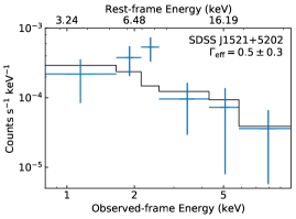
Figure 10: The stacked XMM-Newton EPIC spectrum of SDSS J1521+5202, shown with a folded phabs*powerlaw model in XSPEC.

References

- Antonucci (1993) Antonucci R., 1993, ARA&A, 31, 473
- Arnaud (1996) Arnaud K. A., 1996, XSPEC: The First Ten Years. p. 17
- Baldwin (1977) Baldwin J. A., 1977, ApJ, 214, 679
- Bellm et al. (2019) Bellm E. C., et al., 2019, PASP, 131, 018002
- Boller et al. (1997) Boller T., Brandt W. N., Fabian A. C., Fink H. H., 1997, MNRAS, 289, 393
- Boller et al. (2016) Boller T., Freyberg M. J., Trümper J., Haberl F., Voges W., Nandra K., 2016, A&A, 588, A103
- Boller et al. (2021) Boller T., et al., 2021, A&A, 647, A6
- Brandt et al. (2000) Brandt W. N., Laor A., Wills B. J., 2000, ApJ, 528, 637
- Brightman et al. (2013) Brightman M., et al., 2013, MNRAS, 433, 2485
- Broos et al. (2007) Broos P. S., Feigelson E. D., Townsley L. K., Getman K. V., Wang J., Garmire G. P., Jiang Z., Tsuboi Y., 2007, ApJS, 169, 353
- Chen et al. (2018) Chen C. T. J., et al., 2018, MNRAS, 478, 2132
- Dai et al. (2018) Dai L., McKinney J. C., Roth N., Ramirez-Ruiz E., Miller M. C., 2018, ApJ, 859, L20
- Diamond-Stanic et al. (2009) Diamond-Stanic A. M., et al., 2009, ApJ, 699, 782
- Dickey & Lockman (1990) Dickey J. M., Lockman F. J., 1990, ARA&A, 28, 215
- Done & Jin (2016) Done C., Jin C., 2016, MNRAS, 460, 1716
- Elvis (2012) Elvis M., 2012, in Chartas G., Hamann F., Leighly K. M., eds, Astronomical Society of the Pacific Conference Series Vol. 460, AGN Winds in Charleston. p. 186 (arXiv:1201.3520)
- Fan et al. (1999) Fan X., et al., 1999, ApJ, 526, L57
- Fan et al. (2009) Fan L. L., Wang H. Y., Wang T., Wang J., Dong X., Zhang K., Cheng F., 2009, ApJ, 690, 1006
- Feigelson & Nelson (1985) Feigelson E. D., Nelson P. I., 1985, ApJ, 293, 192
- Fruscione et al. (2006) Fruscione A., et al., 2006, CIAO: Chandra’s data analysis system. p. 62701V, doi:10.1117/12.671760
- Gallagher et al. (2002) Gallagher S. C., Brandt W. N., Chartas G., Garmire G. P., Sambruna R. M., 2002, ApJ, 569, 655
- Gallagher et al. (2006) Gallagher S. C., Brandt W. N., Chartas G., Priddey R., Garmire G. P., Sambruna R. M., 2006, ApJ, 644, 709
- Garmire et al. (2003) Garmire G. P., Bautz M. W., Ford P. G., Nousek J. A., Ricker George R. J., 2003, Advanced CCD imaging spectrometer (ACIS) instrument on the Chandra X-ray Observatory. pp 28–44, doi:10.1117/12.461599
- Gehrels (1986) Gehrels N., 1986, ApJ, 303, 336
- Hagino et al. (2016) Hagino K., Odaka H., Done C., Tomaru R., Watanabe S., Takahashi T., 2016, MNRAS, 461, 3954
- Hamann et al. (2018) Hamann F., Chartas G., Reeves J., Nardini E., 2018, MNRAS, 476, 943
- Hewett & Wild (2010) Hewett P. C., Wild V., 2010, MNRAS, 405, 2302
- Jiang et al. (2014) Jiang Y.-F., Stone J. M., Davis S. W., 2014, ApJ, 796, 106
- Jiang et al. (2019) Jiang Y.-F., Stone J. M., Davis S. W., 2019, ApJ, 880, 67
- Just et al. (2007) Just D. W., Brandt W. N., Shemmer O., Steffen A. T., Schneider D. P., Chartas G., Garmire G. P., 2007, ApJ, 665, 1004
- Kelly (2007) Kelly B. C., 2007, ApJ, 665, 1489
- Kraft et al. (1991) Kraft R. P., Burrows D. N., Nousek J. A., 1991, ApJ, 374, 344
- Lane et al. (2011) Lane R. A., et al., 2011, ApJ, 743, 163
- Lavalley et al. (1992) Lavalley M., Isobe T., Feigelson E., 1992, ASURV: Astronomy Survival Analysis Package. p. 245
- Leighly (1999) Leighly K. M., 1999, ApJS, 125, 297
- Luo et al. (2015) Luo B., et al., 2015, ApJ, 805, 122
- MacLeod et al. (2012) MacLeod C. L., et al., 2012, ApJ, 753, 106
- Marlar et al. (2018) Marlar A., et al., 2018, ApJ, 865, 92
- Miniutti & Fabian (2004) Miniutti G., Fabian A. C., 2004, MNRAS, 349, 1435
- Miniutti et al. (2012) Miniutti G., Brandt W. N., Schneider D. P., Fabian A. C., Gallo L. C., Boller T., 2012, MNRAS, 425, 1718
- Netzer (2015) Netzer H., 2015, ARA&A, 53, 365
- Ni et al. (2018) Ni Q., et al., 2018, MNRAS, 480, 5184
- Ni et al. (2020) Ni Q., et al., 2020, ApJ, 889, L37
- O’Brien et al. (2005) O’Brien P. T., Reeves J. N., Simpson C., Ward M. J., 2005, MNRAS, 360, L25
- Park et al. (2006) Park T., Kashyap V. L., Siemiginowska A., van Dyk D. A., Zezas A., Heinke C., Wargelin B. J., 2006, ApJ, 652, 610
- Parker et al. (2021) Parker M. L., et al., 2021, MNRAS,
- Petrucci et al. (2018) Petrucci P. O., Ursini F., De Rosa A., Bianchi S., Cappi M., Matt G., Dadina M., Malzac J., 2018, A&A, 611, A59
- Planck Collaboration et al. (2020) Planck Collaboration et al., 2020, A&A, 641, A6
- Plotkin et al. (2010) Plotkin R. M., et al., 2010, AJ, 139, 390
- Plotkin et al. (2015) Plotkin R. M., et al., 2015, ApJ, 805, 123
- Pu et al. (2020) Pu X., Luo B., Brandt W. N., Timlin J. D., Liu H., Ni Q., Wu J., 2020, ApJ, 900, 141
- Reeves et al. (2020) Reeves J. N., Braito V., Chartas G., Hamann F., Laha S., Nardini E., 2020, ApJ, 895, 37
- Richards et al. (2003) Richards G. T., et al., 2003, AJ, 126, 1131
- Saxton et al. (2008) Saxton R. D., Read A. M., Esquej P., Freyberg M. J., Altieri B., Bermejo D., 2008, A&A, 480, 611
- Schneider et al. (2010) Schneider D. P., et al., 2010, AJ, 139, 2360
- Shemmer et al. (2008) Shemmer O., Brandt W. N., Netzer H., Maiolino R., Kaspi S., 2008, ApJ, 682, 81
- Shen et al. (2011) Shen Y., et al., 2011, ApJS, 194, 45
- Steffen et al. (2006) Steffen A. T., Strateva I., Brandt W. N., Alexand er D. M., Koekemoer A. M., Lehmer B. D., Schneider D. P., Vignali C., 2006, AJ, 131, 2826
- Strateva et al. (2005) Strateva I. V., Brandt W. N., Schneider D. P., Vanden Berk D. G., Vignali C., 2005, AJ, 130, 387
- Tananbaum et al. (1979) Tananbaum H., et al., 1979, ApJ, 234, L9
- Timlin et al. (2020a) Timlin J. D., Brandt W. N., Ni Q., Luo B., Pu X., Schneider D. P., Vivek M., Yi W., 2020a, MNRAS, 492, 719
- Timlin et al. (2020b) Timlin John D. I., Brandt W. N., Zhu S., Liu H., Luo B., Ni Q., 2020b, MNRAS, 498, 4033
- Timlin et al. (2021) Timlin John D. I., Brandt W. N., Laor A., 2021, MNRAS, 504, 5556
- Vanden Berk et al. (2001) Vanden Berk D. E., et al., 2001, AJ, 122, 549
- Wang et al. (2014) Wang J.-M., Qiu J., Du P., Ho L. C., 2014, ApJ, 797, 65
- Welsh et al. (2011) Welsh B. Y., Wheatley J. M., Neil J. D., 2011, A&A, 527, A15
- Wu et al. (2011) Wu J., et al., 2011, ApJ, 736, 28
- Wu et al. (2012) Wu J., Brandt W. N., Anderson S. F., Diamond-Stanic A. M., Hall P. B., Plotkin R. M., Schneider D. P., Shemmer O., 2012, ApJ, 747, 10
- Xue et al. (2011) Xue Y. Q., et al., 2011, ApJS, 195, 10