TTP22-009, P3H-22-016

Massive vector form factors to three loops

Abstract

We compute the three-loop non-singlet corrections to the photon-quark form factors taking into account the full dependence on the virtuality of the photon and the quark mass. We combine the method of differential equations in an effective way with expansions around regular and singular points. This allows us to obtain results for the form factors with an accuracy of about eight to twelve digits in the whole kinematic range.

Introduction. Form factors are fundamental objects in Quantum Chromodynamics (QCD) with a variety of applications. On the one hand, they are the simplest objects which show a non-trivial infrared struture and thus form factors are often used to develop and test all-order theorems about the infrared singularities of scattering amplitudes in QCD (see, e.g., Refs. Mitov:2006xs ; Becher:2009kw ; Beneke:2009rj ). On the other hand, form factors play a crucial role as building blocks in a number of observables which range from low energies to cross sections at the Large Hadron Collider (LHC) at CERN. They describe the universal structure of the $(Z^{\star},\gamma^{\star})\to\bar{Q}Q$ vertex function, involving two on-shell quarks $Q$ and vector or axial-vector couplings of the vector bosons. Massive form factors enter several processes involving heavy quarks at hadron and $e^{+}e^{-}$ colliders, such as $\bar{t}t$ production Moch:2008qy ; Kidonakis:2008mu ; Moortgat-Pick:2015lbx and gauge and Higgs boson decays Bernreuther:2005gw ; Bernreuther:2018ynm ; Behring:2019oci , which clearly require the inclusion of mass effects. Such processes can probe deviations of the quark couplings from their values in the Standard Model. Form factors contribute to the all-virtual corrections to cross sections.

In Quantum Electrodynamics (QED) lepton masses are often kept to regulate collinear singularities. Therefore massive form factors take part also in the differential cross section of low-energy lepton scatterings as for instance the elastic $e$-$p$ scattering Bucoveanu:2018soy ; Banerjee:2020rww , one of the main avenues for proton radius measurements A1:2010nsl ; Xiong:2019umf , or the $\mu$-$e$ scattering CarloniCalame:2020yoz ; Banerjee:2020rww , a process able to determine the leading hadronic contribution to the muon anomalous magnetic moment CarloniCalame:2015obs ; Abbiendi:2016xup ; loimuone ; Banerjee:2020tdt .

For massless quarks three-loop corrections to the photon-quark form factor have been computed more than 10 years ago Baikov:2009bg (see also Refs. Lee:2010ik ; Gehrmann:2010ue ; Gehrmann:2010tu ; vonManteuffel:2015gxa ) and only very recently the complete four loop results became available Lee:2021uqq ; LMSSSS22 . Massive quark form factors are known at two-loop order from Refs. Mastrolia:2003yz ; Bonciani:2003ai ; Bernreuther:2004ih ; Gluza:2009yy ; Henn:2016tyf ; Ahmed:2017gyt ; Ablinger:2017hst ; Lee:2018nxa . At three loops only partial results are available, namely all planar contributions needed for the large-$N_{c}$ limit (where $N_{c}$ is the number of colours in QCD) Henn:2016tyf ; Ablinger:2018yae and the fermionic contributions with closed massless quark loops Lee:2018nxa . For the contribution involving massive closed fermion loops a deep expansion with at least 2000 terms around the on-shell photon limit has been computed in Ref. Blumlein:2019oas .

The available results show an involved analytic structure containing iterated integrals with the letters $x$, $1-x$, $1+x$ and $x-e^{i\pi/3}$, where the relation between $x$ and the photon virtuality $s=q^{2}$ is given by

$$\frac{q^{2}}{m^{2}} = -\frac{(1-x)^{2}}{x}\,,$$ (1)

with $m$ the mass of the heavy quark. A numerical evaluation of the analytic expressions is possible using, e.g., ginac Bauer:2000cp ; Vollinga:2004sn . However, depending on the phase space point it might be time consuming and/or its numerical accuracy is limited to a few digits only. Thus, in practice, one often resolves to the construction of approximations which enable a fast numerical evaluation. Moreover, the three-loop results for the colour structures which are not yet available in analytic form cannot be expressed in terms of simple iterated integrals. Rather, so-called elliptic integrals are present as the fundamental building blocks. Currently there is no ready-to-use approach for the numerical evaluation of the corresponding mathematical functions and thus especially here numerical approximations are needed.

In this Letter we present results for the three-loop form factor with an external vector current. We consider QCD with one massive and $n_{l}$ massless flavours and compute the non-singlet contribution, where the external quarks directly couple to the current, see also the sample Feynman diagrams in Fig. 1. We perform the reduction to master integrals and establish the differential equations for the latter. They are used in order to construct expansions around singular and regular points using analytic results at $s=0$ as initial condition. In our calculation we keep the symbols for the Casimir operators of SU$(N_{c})$ and thus obtain results for each individual colour factor.

There are other methods which are based on difference or differential equations accompanied by expansions Laporta:2001dd ; Boughezal:2007ny ; Blumlein:2017dxp ; Liu:2017jxz ; Lee:2017qql ; Moriello:2019yhu ; Hidding:2020ytt ; Dubovyk:2022frj . However, some of them have only been applied to individual master integrals and they are still lacking the proof that they can handle non-trivial physical problems with a few hundred master integrals. In this paper we apply the method of Ref. Fael:2021kyg to a non-trivial physical quantity and show that numerically precise results can be obtained in the whole parameter space.

Calculation. We consider the photon-quark vertex and define the Dirac and Pauli form factors as

$$\Gamma_{\mu}(q_{1},q_{2}) = F_{1}(q^{2})\gamma_{\mu}-\frac{i}{2m}F_{2}(q^{2})\sigma_{\mu\nu}q^{\nu}\,,$$ (2)

with incoming momentum $q_{1}$, outgoing momentum $q_{2}$ and $q=q_{1}-q_{2}$. The external quarks are on-shell and we have $\sigma^{\mu\nu}=i[\gamma^{\mu},\gamma^{\nu}]/2$. The colour factor is a simple Kronecker delta in the fundamental colour indices of the external quarks and it is suppressed for convenience. $F_{1}$ and $F_{2}$ can easily be obtained by applying appropriate projectors.

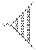
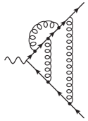
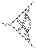
(a)	(b)	(c)

Figure 1: Sample Feynman diagrams for the vector form factors at three loops. Solid and curly lines denote quarks and gluons, respectively. The external photon is represented by a wavy line.

Sample Feynman diagrams are shown in Fig. 1. We generate the amplitudes with qgraf Nogueira:1991ex and use q2e and exp Harlander:1997zb ; Seidensticker:1999bb ; q2eexp to rewrite the output to FORM Kuipers:2012rf notation and map each diagram to a predefined integral family. In this way we can express $F_{1}$ and $F_{2}$ as a linear combination of scalar functions with twelve indices where nine correspond to the exponents of propagators and the remaining three to the exponents of irreducible numerators.

For each integral family we use Kira Maierhofer:2017gsa ; Klappert:2020nbg with Fermat fermat to reduce the scalar functions to master integrals. In this step we take care to choose a good basis such that for each entry in our integral tables the dependence on the space-time dimension $d=4-2\epsilon$ and the kinematic variables $s$ and $m^{2}$ factorizes in the denominators. This is done with the help of an improved version of the program developed in Ref. Smirnov:2020quc . Kira is also used to minimize the number of master integrals over all families. This allows us to express $F_{1}$ and $F_{2}$ in terms of 422 master integrals.

In a next step we establish differential equations for the master integrals using LiteRed Lee:2012cn ; Lee:2013mka and Kira and use the results for $s\to 0$ as initial conditions. In fact, the construction of the solution can be organized such that the naive limit $s=0$ of a subset of the 422 master integrals is sufficient to fix all unknown constants.

In the limit $s=0$ the vertex integrals reduce to two-point on-shell integrals, which have been studied in Refs. Laporta:1996mq ; Melnikov:2000qh . We use the results for the corresponding master integrals from Ref. Lee:2010ik which are available up to weight 7. Due to spurious poles in $\epsilon$ some of the on-shell master integrals are needed to higher weight which can be constructed with the help of Ref. Lee:2015eva and PSLQ PSLQ (see also Ref. Blumlein:2019oas ). For the current calculation a subset of integrals was needed up to weight 9.

After fixing the initial conditions we can use the differential equations to obtain for each master integral an expansion in $s/m^{2}$ up to $(s/m^{2})^{75}$. For all other expansions described below we have computed 50 expansion terms. In this context the use of finite fields with a special version of Kira and FireFly Klappert:2019emp ; Klappert:2020aqs was essential for our calculation. Starting from $s=0$ we move both to negative and positive values of $s$. To do so we choose values $s_{0}/m^{2}=1$ and $s_{0}/m^{2}=-4$ and construct generic expansions with the help of the differential equations. They are matched to the $s=0$ expansion by evaluating the latter numerically at $s/m^{2}=1/2$ and $s/m^{2}=-2$, respectively. This provides initial conditions for the $s_{0}$ expansions. In total we construct expansions around the following 30 values

$$\frac{s_{0}}{m^{2}}\!\in\!\{-\infty,-32,-28,-24,-16,-12,-8,-4,0,1,2,5/2,$$

$$\!\!3,7/2,4,9/2,5,6,7,8,10,12,14,15,16,17,19,22,28,40\}$$

(3)

and perform the matching step-by-step starting from $s=0$. In this way we can cover the whole $s/m^{2}$ plane. For more details on the “expansion and matching” method we refer to Ref. Fael:2021kyg .

At first sight it seems that the variable $x$ introduced in Eq. (1) is the proper variable to perform the expansions, since the characteristic points $s/m^{2}=0,4,\infty$ correspond to $x=1,-1,0$. However, in practice it is more advantageous to work in $s/m^{2}$. This is also connected to the new threshold at $s/m^{2}=16$ which appears for the first time at three loops. It is mapped to $x=4\sqrt{3}-7\approx-0.072$ which limits the radius of convergence of the variable $x$.

Let us in the following comment on the choice of $s_{0}$ in Eq. (3). Some values correspond to a particular kinematic situation: $s/m^{2}=4$ and $16$ correspond to the two- and four-particle thresholds and $m^{2}/s=0$ to the high energy limit. Furthermore, as mentioned above, we compute the initial conditions for $s=0$. To guarantee sufficient accuracy over the whole $s/m^{2}$ range we have introduced further expansions for positive and negative values of $s$. In the differential equations we observe further singularities for $s/m^{2}\in\{-4,-2,-1,-1/2,1/2,1,2,3,16/3\}$. However, they are spurious since the form factors are regular for these values of $s$. Nevertheless, for some of them we have constructed an expansion of the master integrals.

For all expansions the convergence around a given value $s_{0}$ is only guaranteed up to the next singular point in the complex $s$ plane. For example for $s_{0}/m^{2}=22$ we have convergence for $16<s/m^{2}<28$ and for $s_{0}/m^{2}=-4$ for $-12<s/m^{2}<4$. Note that $s/m^{2}=4,16$ and $\infty$ are singular points of the differential equation which require a power-log expansion. Furthermore, for $s/m^{2}=4$ and $16$ we have an expansion in $\sqrt{4-s/m^{2}}$ and $\sqrt{16-s/m^{2}}$, respectively. For all other points simple Taylor expansions are sufficient.

Often the convergence of a series expansion can be enhanced by switching to a different expansion parameter. One powerful method is based on Möbius transformations as has already been discussed in Ref. Lee:2017qql . Assume, we want to expand around the point $x_{k}$ and there are singular points of the differential equations at $x_{k-1}$ and $x_{k+1}$ with $x_{k-1}<x_{k}<x_{k+1}$. Naively the radius of convergence is limited by the distance to the closer singular point. However, the variable transformation

$$y_{k}=\frac{(x-x_{k})(x_{k+1}-x_{k-1})}{(x-x_{k+1})(x_{k-1}-x_{k})+(x-x_{k-1})(x_{k+1}-x_{k})}$$ (4)

maps the points $x_{k-1}$, $x_{k}$, $x_{k+1}$ to $-1$, $0$, $1$. The reach of the series expansion is therefore extended in the direction of the farthest singularity although the convergence at the boundaries can be quite slow. We find this mapping indispensable when constructing regular series expansions close to singular points.

The form factors $F_{1}$ and $F_{2}$ develop both ultraviolet and infrared divergences. The former are taken care of by counterterms for the wave functions and mass of the heavy quarks, which we renormalize on-shell. Furthermore, the strong coupling constant is renormalized in the $\overline{\rm MS}$ scheme. The remaining infrared poles are described by a universal function independent of the external current, the cusp anomalous dimension $\Gamma_{\rm cusp}$, which has been computed to three-loop accuracy in Refs. Grozin:2014hna ; Grozin:2015kna . It is used to construct a $Z$ factor (see, e.g., Ref. Lee:2018rgs ) such that the combination

$$F_{1,2}=ZF_{1,2}^{f}$$ (5)

leads to the ultraviolet and infrared finite form factors $F_{1,2}^{f}$. We introduce their perturbative expansion as

$$F_{1,2}^{f} = \sum_{n\geq 0}F_{1,2}^{f,(n)}\left(\frac{\alpha_{s}}{\pi}\right)^{n}\,,$$ (6)

where $F_{1}^{f,(0)}=1$ and $F_{2}^{f,(0)}=0$. Since $Z$ is expressed in terms of the strong coupling in the effective $n_{l}$-flavour theory we have $\alpha_{s}\equiv\alpha_{s}^{(n_{l})}(\mu)$ in Eq. (6). In the next Section we discuss results for $F_{1}^{f,(3)}$ and $F_{2}^{f,(3)}$.

Results. The results from our calculation are expansions around the values $s_{0}$ in Eq. (3). Thus, we can define the form factors $F_{1}$ and $F_{2}$ piecewise by these expansions. We choose for the renormalization scale $\mu^{2}=m^{2}$.

In the following we concentrate on $F_{1}$ and present results for the renormalized and infrared-subtracted form factor. In Fig. 2 we illustrate the results for the three non-fermionic colour structures $C_{F}^{3}$, $C_{F}^{2}C_{A}$, $C_{F}C_{A}^{2}$, where $C_{F}$ and $C_{A}$ are the Casimir operators of the fundamental and the adjoint representation, respectively, and present results for $s<0$ and $s>4m^{2}$. For $s=0$ we have $F_{1}=0$ as can be seen in plot (a). In plot (b) one observes the influence of the Coulomb singularity even for $s/m^{2}\approx 10$. The four-particle threshold is much less pronounced. In the high-energy region, both for $s>0$ and $s<0$ the form factor contains logarithms up to sixth order.

We estimate the accuracy of our result from the numerical pole cancellations of the renormalized and infrared subtracted form factor. For $s>4m^{2}$ the quadratic and linear $1/\epsilon$ poles cancel with a relative precision of $10^{-12}$ and $10^{-10}$, respectively. Assuming a similar progression we estimate that for the finite term we have at least eight significant digits for the coefficients of each colour factor. In the regions $0<s<4m^{2}$ and $s<0$ the accuracy is significantly higher and in general exeeds twelve significant digits. Also for the fermionic colour structures a notably higher accuracy is reached.

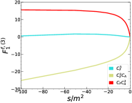
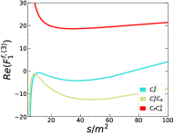
(a)	(b)

Figure 2: The colour structures $C_{F}^{3}$, $C_{F}^{2}C_{A}$, $C_{F}C_{A}^{2}$ of $F_{1}^{f}$ as a function of $s$. We show results for $s<0$ (a) and $s>4m^{2}$ (b).

In a next step we consider the special kinematic points $s=0,4m^{2},16m^{2}$ and $\pm\infty$ and present (numerical) expansions using the genuine results of our approximation methods. In this Letter we restrict ourselves to the non-fermionic colour factors. In the supplemenatry material we present results for the contributions which contain a closed heavy quark loop. The remaining fermionic contributions are available in the literature Lee:2018nxa ; Lee:2018rgs .

In the static limit we construct an analytic expansion up to $s^{67}$ from the boundary values at $s=0$. The first two expansion terms are given by

$$F_{1}^{f,(3)}\Big{|}_{s\to 0}=\Bigg{\{}C_{A}C_{F}^{2}\Bigg{[}\frac{19a_{4}}{2}-\frac{\pi^{2}\zeta_{3}}{9}+\frac{17725\zeta_{3}}{3456}-\frac{55\zeta_{5}}{32}+\frac{19l_{2}^{4}}{48}-\frac{97}{720}\pi^{2}l_{2}^{2}+\frac{29\pi^{2}l_{2}}{240}-\frac{347\pi^{4}}{17280}-\frac{4829\pi^{2}}{10368}+\frac{707}{288}\Bigg{]}$$ (7)

$$\mbox{}+C_{A}^{2}C_{F}\Bigg{[}-a_{4}+\frac{7\pi^{2}\zeta_{3}}{96}+\frac{4045\zeta_{3}}{5184}-\frac{5\zeta_{5}}{64}-\frac{l_{2}^{4}}{24}+\frac{67}{360}\pi^{2}l_{2}^{2}-\frac{5131\pi^{2}l_{2}}{2880}+\frac{67\pi^{4}}{8640}+\frac{172285\pi^{2}}{186624}-\frac{7876}{2187}\Bigg{]}$$

$$\mbox{}+C_{F}^{3}\Bigg{[}-15a_{4}-\frac{17\pi^{2}\zeta_{3}}{24}-\frac{18367\zeta_{3}}{1728}+\frac{25\zeta_{5}}{8}-\frac{5l_{2}^{4}}{8}-\frac{19}{40}\pi^{2}l_{2}^{2}+\frac{4957\pi^{2}l_{2}}{720}+\frac{3037\pi^{4}}{25920}-\frac{24463\pi^{2}}{7776}+\frac{13135}{20736}\Bigg{]}\Bigg{\}}\frac{s}{m^{2}}$$

$$\mbox{}+{\cal O}\left(\frac{s^{2}}{m^{4}}\right)+\mbox{fermionic contributions}\,,$$

where $l_{2}=\log(2)$, $a_{4}=\mbox{Li}_{4}(1/2)$ and $\zeta_{n}$ is Riemann’s zeta function evaluated at $n$.

The first two terms for the high-energy expansion of the non-fermionic colour structures read

$$F_{1}^{f,(3)}\Big{|}_{s\to-\infty}=4.7318C_{F}^{3}-20.762C_{F}^{2}C_{A}+8.3501C_{F}C_{A}^{2}+\Big{[}3.4586C_{F}^{3}-4.0082C_{F}^{2}C_{A}-6.3561C_{F}C_{A}^{2}\Big{]}l_{s}$$ (8)

$$\mbox{}+\Big{[}1.4025C_{F}^{3}+0.51078C_{F}^{2}C_{A}-2.2488C_{F}C_{A}^{2}\Big{]}l_{s}^{2}+\Big{[}0.062184C_{F}^{3}+0.90267C_{F}^{2}C_{A}-0.42778C_{F}C_{A}^{2}\Big{]}l_{s}^{3}$$

$$\mbox{}+\Big{[}-0.075860C_{F}^{3}+0.20814C_{F}^{2}C_{A}-0.035011C_{F}C_{A}^{2}\Big{]}l_{s}^{4}+\Big{[}{-0.023438}C_{F}^{3}+0.019097C_{F}^{2}C_{A}\Big{]}l_{s}^{5}$$

$$\mbox{}+\Big{[}{-0.0026042}C_{F}^{3}\Big{]}l_{s}^{6}+\Big{\{}-92.918C_{F}^{3}+123.65C_{F}^{2}C_{A}-47.821C_{F}C_{A}^{2}+\Big{[}-10.381C_{F}^{3}+2.3223C_{F}^{2}C_{A}$$

$$\mbox{}+17.305C_{F}C_{A}^{2}\Big{]}l_{s}+\Big{[}4.9856C_{F}^{3}-19.097C_{F}^{2}C_{A}+8.0183C_{F}C_{A}^{2}\Big{]}l_{s}^{2}+\Big{[}{3.0499}C_{F}^{3}{-6.8519}C_{F}^{2}C_{A}+1.9149C_{F}C_{A}^{2}\Big{]}l_{s}^{3}$$

$$\mbox{}+\Big{[}0.67172C_{F}^{3}-0.91213C_{F}^{2}C_{A}+0.24069C_{F}C_{A}^{2}\Big{]}l_{s}^{4}+\Big{[}0.13229C_{F}^{3}-0.051389C_{F}^{2}C_{A}+0.0043403C_{F}C_{A}^{2}\Big{]}l_{s}^{5}$$

$$\mbox{}+\Big{[}0.0041667C_{F}^{3}-0.0010417C_{F}^{2}C_{A}-0.00052083C_{F}C_{A}^{2}\Big{]}l_{s}^{6}\Big{\}}\frac{m^{2}}{s}+{\cal O}\left(\frac{m^{4}}{s^{2}}\right)+\mbox{fermionic contributions}\,,$$

with $l_{s}=\log(m^{2}/(-s-i\delta))$. The leading logarithmic contributions of the order $\alpha_{s}^{n}\log^{2n}(m^{2}/s)$ are given by the Sudakov exponent Sudakov:1954sw ; Frenkel:1976bj $\mbox{exp}[-C_{F}\alpha_{s}/(4\pi)\times\log^{2}(m^{2}/s)]$ which is reproduced by our expansions. In fact, in our calculation we can even reconstruct the analytic results of the coefficients which are given by

$$F_{1}^{f,{(3)}}\!\!=\!-\frac{C_{F}^{3}}{384}l_{s}^{6}+\frac{m^{2}}{s}\left(\frac{C_{F}^{3}}{240}-\frac{C_{F}^{2}C_{A}}{960}-\frac{C_{F}C_{A}^{2}}{1920}\right)l_{s}^{6}\!+\ldots$$

(9)

In Eq. (8) they are shown in numeric form. Note that also the leading logarithms of the mass corrections $m^{2}/s$ perfectly agree with Ref. Liu:2017axv where the results in Eq. (9) have been obtained using an involved asymptotic expansion of the three-loop vertex diagrams. Our approach provides the whole tower of logarithms and also higher order $m^{2}/s$ contributions. We estimate the accuracy of the non-logarithmic term in Eq. (8) to ten digits. For the subleading terms the accuracy decreases. Note, however, that we use the $s\to\infty$ expansion only for $|s/m^{2}|\gtrsim 45$ and that $1/45^{3}\approx{\cal O}(10^{-5})$.

Let us next discuss the thresholds at $s=4m^{2}$ and $s=16m^{2}$. Close to the two-particle threshold $F_{1}$ develops the famous Coulomb singularity with negative powers in the velocity of the produced quarks, $\beta=\sqrt{1-4m^{2}/s}$, up to third order multiplied by $\log(\beta)$ terms. Close to threshold it is interesting to consider the combination of $F_{1}$ and $F_{2}$

$$\frac{3}{2}\Delta = |F_{1}+F_{2}|^{2}+\frac{|(1-\beta^{2})F_{1}+F_{2}|^{2}}{2(1-\beta^{2})}\,,$$ (10)

which is closely related to the cross section of heavy quark production in electron positron annihilation via $\sigma(e^{+}e^{-}\to Q\bar{Q})=\sigma_{0}\beta 3\Delta/2$ with $\sigma_{0}=4\pi\alpha^{2}Q_{Q}^{2}/(3s)$, where $\alpha$ is the fine structure constant and $Q_{Q}$ is the fractional charge of the massive quark $Q$. For $\beta\to 0$ real radiation is suppressed by two powers of $\beta$ which allows us to provide the first two terms in the expansion for each colour factor. Our result for the third order correction $\Delta^{(3)}$ reads

$$\Delta^{(3)}=C_{F}^{3}\bigl{[}-\frac{32.470}{\beta^{2}}+\frac{1}{\beta}\bigl{(}14.998-32.470l_{2\beta}\bigr{)}\bigr{]}+C_{A}^{2}C_{F}\frac{1}{\beta}\bigl{[}16.586l^{2}_{2\beta}-22.572l_{2\beta}+42.936\bigr{]}$$

$$+C_{A}C_{F}^{2}\bigl{[}\frac{1}{\beta^{2}}\bigl{(}-29.764l_{2\beta}-7.770339\bigr{)}+\frac{1}{\beta}\bigl{(}-12.516l_{2\beta}-11.435\bigr{)}\bigr{]}+\mathcal{O}(\beta^{0})+\mbox{fermionic contributions}\,,$$ (11)

with $l_{2\beta}=\log(2\beta)$. Our numerical results reproduce the analytic expressions from Ref. Kiyo:2009gb (see also Refs. Pineda:2006ri ; Hoang:2008qy ) with at least 13 digits accuracy.

Four-particle thresholds are present in diagrams which contain a closed heavy quark loop but also in purely gluonic diagrams like the one in Fig. 1(b). Interestingly it has a smooth behaviour. In fact, we observe the first non-analytic terms at order $(\beta_{4})^{9}$ with $\beta_{4}=\sqrt{1-16m^{2}/s}$. Note that the massive four-particle phase-space, which is one of our master integrals, already provides a factor $(\beta_{4})^{7}$. Furthermore, our expansions of $F_{1}$ and $F_{2}$ up to $(\beta_{4})^{50}$ do not contain any $\log\beta_{4}$ terms although many of the master integrals contain such terms.

Finally, we want to mention that we have performed the calculation for general QCD gauge parameter $\xi$ and have checked that $\xi$ cancels in the renormalized form factors. Note that both the bare three-loop expressions and the quark mass counterterm contributions depend on $\xi$. Furthermore, we can specify our result to the large-$N_{c}$ limit and compare against the exact results from Ref. Henn:2016tyf . In this limit only about 90 planar master integrals contribute and we observe a significantly increased precision of our result. In fact, in the whole $s/m^{2}$ region we can reproduce the exact result with at least 14 digits.

Conclusions. In this Letter we present for the first time results for the non-singlet three-loop massive photon-quark form factors taking into account all colour structures. We use the methods based on “expansion and matching” as introduced in Ref. Fael:2021kyg and obtain numerical approximations in the whole $s/m^{2}$ range. Based on the comparison to the partially known exact results and on internal cross checks of the method we estimate the accuracy to at least eight significant digits above the $s=4m^{2}$ threshold and to about twelve digits below. Note that, if required, a systematic improvement is possible by adding more intermediate matching points. The application to a physical quantity with a non-trivial analytic structure shows the effectiveness of our method.

Acknowledgements. We thank Roman Lee for discussions about the Möbius transformations and Alexander Smirnov and Vladimir Smirnov for discussions about the basis change for the master integrals and providing an improved version of the Mathematica code from Ref. Smirnov:2020quc . This research was supported by the Deutsche Forschungsgemeinschaft (DFG, German Research Foundation) under grant 396021762 — TRR 257 “Particle Physics Phenomenology after the Higgs Discovery”. The Feynman diagrams were drawn with the help of Axodraw Vermaseren:1994je and JaxoDraw Binosi:2003yf .

Supplementary material

To complete the presentation of the main part of the Letter we provide in the following results for $F_{1}$ involving a closed heavy quark for $s\to 0$, $s\to-\infty$ and $s\to 4m^{2}$. For such contributions one often introduces the tag $n_{h}$, which means that we present result for the colour factors $C_{F}^{2}T_{F}n_{h}$, $C_{F}C_{A}T_{F}n_{h}$, $C_{F}T_{F}^{2}n_{h}^{2}$ and $C_{F}T_{F}^{2}n_{h}n_{l}$.

For $s\to 0$ we have

$$F_{1}^{f,(3),n_{h}}\Big{|}_{s\to 0}=\Bigg{\{}C_{A}C_{F}T_{F}n_{h}\Bigg{(}\frac{17a_{4}}{6}-\frac{\pi^{2}\zeta_{3}}{18}+\frac{1775\zeta_{3}}{864}+\frac{5\zeta_{5}}{12}+\frac{17l_{2}^{4}}{144}-\frac{17}{144}\pi^{2}l_{2}^{2}-\frac{149\pi^{2}l_{2}}{108}+\frac{803\pi^{4}}{51840}$$ (12)

$$\mbox{}+\frac{4813\pi^{2}}{5184}-\frac{23089}{5184}\Bigg{)}+C_{F}^{2}T_{F}n_{h}\Bigg{(}-\frac{32a_{4}}{9}+\frac{1441\zeta_{3}}{1728}-\frac{4l_{2}^{4}}{27}+\frac{4}{27}\pi^{2}l_{2}^{2}-\frac{2\pi^{2}l_{2}}{9}-\frac{13\pi^{4}}{1620}+\frac{1057\pi^{2}}{2430}-\frac{2273}{1296}\Bigg{)}$$

$$\mbox{}+C_{F}T_{F}^{2}n_{h}n_{l}\Bigg{(}\frac{7\zeta_{3}}{48}-\frac{1}{24}\pi^{2}l_{2}-\frac{71\pi^{2}}{1296}+\frac{1261}{1944}\Bigg{)}+C_{F}T_{F}^{2}n_{h}^{2}\Bigg{(}-\frac{28\zeta_{3}}{27}+\frac{4\pi^{2}}{135}+\frac{11257}{11664}\Bigg{)}\Bigg{\}}\frac{s}{m^{2}}+{\cal O}\left(\frac{s^{2}}{m^{4}}\right)\,.$$

In the high-energy limit the $n_{h}$ contributions are given by

$$F_{1}^{f,(3),n_{h}}\Big{|}_{s\to-\infty}=-1.54208C_{F}T_{F}^{2}n_{h}^{2}-4.1144C_{F}T_{F}^{2}n_{h}n_{l}-3.2872C_{F}^{2}T_{F}n_{h}+10.425C_{F}C_{A}T_{F}n_{h}$$ (13)

$$\mbox{}+\Big{[}-1.2844C_{F}T_{F}^{2}n_{h}^{2}-2.8537C_{F}T_{F}^{2}n_{h}n_{l}-2.8785C_{F}^{2}T_{F}n_{h}+7.6917C_{F}C_{A}T_{F}n_{h}\Big{]}l_{s}$$

$$\mbox{}+\Big{[}-0.40466C_{F}T_{F}^{2}n_{h}^{2}-0.80931C_{F}T_{F}^{2}n_{h}n_{l}-1.8900C_{F}^{2}T_{F}n_{h}+2.2962C_{F}C_{A}T_{F}n_{h}\Big{]}l_{s}^{2}$$

$$\mbox{}+\Big{[}-0.058642C_{F}T_{F}^{2}n_{h}^{2}-0.11728C_{F}T_{F}^{2}n_{h}n_{l}-0.55727C_{F}^{2}T_{F}n_{h}+0.33008C_{F}C_{A}T_{F}n_{h}\Big{]}l_{s}^{3}$$

$$\mbox{}+\Big{[}-0.0046296C_{F}T_{F}^{2}n_{h}^{2}-0.0092593C_{F}T_{F}^{2}n_{h}n_{l}-0.086806C_{F}^{2}T_{F}n_{h}+0.025463C_{F}C_{A}T_{F}n_{h}\Big{]}l_{s}^{4}$$

$$\mbox{}+\Big{[}-0.0069444C_{F}^{2}T_{F}n_{h}\Big{]}l_{s}^{5}+\Big{\{}11.898C_{F}T_{F}^{2}n_{h}^{2}+18.981C_{F}T_{F}^{2}n_{h}n_{l}-5.2612C_{F}^{2}T_{F}n_{h}+-52.115C_{F}C_{A}T_{F}n_{h}$$

$$\mbox{}+\Big{[}7.2323C_{F}T_{F}^{2}n_{h}^{2}+8.7158C_{F}T_{F}^{2}n_{h}n_{l}+3.3633C_{F}^{2}T_{F}n_{h}+-25.912C_{F}C_{A}T_{F}n_{h}\Big{]}l_{s}$$

$$\mbox{}+\Big{[}1.8056C_{F}T_{F}^{2}n_{h}^{2}+2.5000C_{F}T_{F}^{2}n_{h}n_{l}+8.4570C_{F}^{2}T_{F}n_{h}-7.8739C_{F}C_{A}T_{F}n_{h}\Big{]}l_{s}^{2}+\Big{[}0.27778C_{F}T_{F}^{2}n_{h}^{2}$$

$$\mbox{}+0.33333C_{F}T_{F}^{2}n_{h}n_{l}+2.3758C_{F}^{2}T_{F}n_{h}-1.4464C_{F}C_{A}T_{F}n_{h}\Big{]}l_{s}^{3}+\Big{[}0.48843C_{F}^{2}T_{F}n_{h}$$

$$\mbox{}-0.067130C_{F}C_{A}T_{F}n_{h}\Big{]}l_{s}^{4}+\Big{[}0.0069444C_{F}^{2}T_{F}n_{h}-0.0034722C_{F}C_{A}T_{F}n_{h}\Big{]}l_{s}^{5}\Big{\}}\frac{m^{2}}{s}+{\cal O}\left(\frac{m^{4}}{s^{2}}\right)\,.$$

For $\beta\to 0$ the results read

$$\Delta^{(3),n_{h}} = C_{F}^{2}T_{F}n_{h}\bigl{[}\frac{2.4792}{\beta}-1.3159l_{2\beta}-2.0339\bigr{]}-C_{A}C_{F}T_{F}n_{h}\bigl{[}0.082247\beta+0.20495\bigr{]}+0.10248C_{F}T_{F}^{2}n_{h}^{2}$$ (14)

$$\mbox{}+C_{F}T_{F}^{2}n_{h}n_{l}\bigl{[}0.87730\beta-0.54050\bigr{]}+\ldots\,,$$

where the ellipses denote higher order terms in $\beta$.

References

- (1) A. Mitov and S.-O. Moch, JHEP 05 (2007), 001 [arXiv:hep-ph/0612149].
- (2) T. Becher and M. Neubert, Phys. Rev. D 79 (2009), 125004 [erratum: Phys. Rev. D 80 (2009), 109901] [arXiv:0904.1021 [hep-ph]].
- (3) M. Beneke, P. Falgari and C. Schwinn, Nucl. Phys. B 828 (2010), 69-101 [arXiv:0907.1443 [hep-ph]].
- (4) S.-O. Moch and P. Uwer, Phys. Rev. D 78 (2008), 034003 [arXiv:0804.1476 [hep-ph]].
- (5) N. Kidonakis and R. Vogt, Phys. Rev. D 78 (2008), 074005 [arXiv:0805.3844 [hep-ph]].
- (6) G. Moortgat-Pick, H. Baer, M. Battaglia, G. Belanger, K. Fujii, J. Kalinowski, S. Heinemeyer, Y. Kiyo, K. Olive, F. Simon et al., Eur. Phys. J. C 75 (2015), 371 [arXiv:1504.01726 [hep-ph]].
- (7) W. Bernreuther, R. Bonciani, T. Gehrmann, R. Heinesch, P. Mastrolia and E. Remiddi, Phys. Rev. D 72 (2005), 096002 [arXiv:hep-ph/0508254].
- (8) W. Bernreuther, L. Chen and Z.-G. Si, JHEP 07 (2018), 159 [arXiv:1805.06658 [hep-ph]].
- (9) A. Behring and W. Bizoń, JHEP 01 (2020), 189 [arXiv:1911.11524 [hep-ph]].
- (10) R.-D. Bucoveanu and H. Spiesberger, Eur. Phys. J. A 55 (2019), 57 [arXiv:1811.04970 [hep-ph]].
- (11) P. Banerjee, T. Engel, A. Signer and Y. Ulrich, SciPost Phys. 9 (2020), 027 [arXiv:2007.01654 [hep-ph]].
- (12) J. C. Bernauer et al. [A1], Phys. Rev. Lett. 105 (2010), 242001 [arXiv:1007.5076 [nucl-ex]].
- (13) W. Xiong, A. Gasparian, H. Gao, D. Dutta, M. Khandaker, N. Liyanage, E. Pasyuk, C. Peng, X. Bai, L. Ye et al., Nature 575 (2019), 147-150.
- (14) C. M. Carloni Calame, M. Chiesa, S. M. Hasan, G. Montagna, O. Nicrosini and F. Piccinini, JHEP 11 (2020), 028 [arXiv:2007.01586 [hep-ph]].
- (15) C. M. Carloni Calame, M. Passera, L. Trentadue and G. Venanzoni, Phys. Lett. B 746 (2015), 325-329 [arXiv:1504.02228 [hep-ph]].
- (16) G. Abbiendi, C. M. Carloni Calame, U. Marconi, C. Matteuzzi, G. Montagna, O. Nicrosini, M. Passera, F. Piccinini, R. Tenchini, L. Trentadue et al., Eur. Phys. J. C 77 (2017), 139 [arXiv:1609.08987 [hep-ex]].
- (17) G. Abbiendi et al., Letter of Intent: The MUonE Project, CERN-SPSC-2019-026 / SPSC-I-252, 2019.
- (18) P. Banerjee, C. M. Carloni Calame, M. Chiesa, S. Di Vita, T. Engel, M. Fael, S. Laporta, P. Mastrolia, G. Montagna, O. Nicrosini et al., Eur. Phys. J. C 80 (2020), 591 [arXiv:2004.13663 [hep-ph]].
- (19) P. A. Baikov, K. G. Chetyrkin, A. V. Smirnov, V. A. Smirnov and M. Steinhauser, Phys. Rev. Lett. 102 (2009), 212002 [arXiv:0902.3519 [hep-ph]].
- (20) R. N. Lee and V. A. Smirnov, JHEP 02 (2011), 102 [arXiv:1010.1334 [hep-ph]].
- (21) T. Gehrmann, E. W. N. Glover, T. Huber, N. Ikizlerli and C. Studerus, JHEP 06 (2010), 094 [arXiv:1004.3653 [hep-ph]].
- (22) T. Gehrmann, E. W. N. Glover, T. Huber, N. Ikizlerli and C. Studerus, JHEP 11 (2010), 102 [arXiv:1010.4478 [hep-ph]].
- (23) A. von Manteuffel, E. Panzer and R. M. Schabinger, Phys. Rev. D 93 (2016), 125014 [arXiv:1510.06758 [hep-ph]].
- (24) R. N. Lee, A. von Manteuffel, R. M. Schabinger, A. V. Smirnov, V. A. Smirnov and M. Steinhauser, Phys. Rev. D 104 (2021), 074008 [arXiv:2105.11504 [hep-ph]].
- (25) R. N. Lee, A. von Manteuffel, R. M. Schabinger, A. V. Smirnov, V. A. Smirnov and M. Steinhauser, MSUHEP-22-003, P3H-22-014, TTP22-008.
- (26) P. Mastrolia and E. Remiddi, Nucl. Phys. B 664 (2003), 341-356 [arXiv:hep-ph/0302162].
- (27) R. Bonciani, P. Mastrolia and E. Remiddi, Nucl. Phys. B 676 (2004), 399-452 [arXiv:hep-ph/0307295].
- (28) W. Bernreuther, R. Bonciani, T. Gehrmann, R. Heinesch, T. Leineweber, P. Mastrolia and E. Remiddi, Nucl. Phys. B 706 (2005), 245-324 [arXiv:hep-ph/0406046].
- (29) J. Gluza, A. Mitov, S. Moch and T. Riemann, JHEP 07 (2009), 001 [arXiv:0905.1137 [hep-ph]].
- (30) J. Henn, A. V. Smirnov, V. A. Smirnov and M. Steinhauser, JHEP 01 (2017), 074 [arXiv:1611.07535 [hep-ph]].
- (31) T. Ahmed, J. M. Henn and M. Steinhauser, JHEP 06 (2017), 125 [arXiv:1704.07846 [hep-ph]].
- (32) J. Ablinger, A. Behring, J. Blümlein, G. Falcioni, A. De Freitas, P. Marquard, N. Rana and C. Schneider, Phys. Rev. D 97 (2018), 094022 [arXiv:1712.09889 [hep-ph]].
- (33) R. N. Lee, A. V. Smirnov, V. A. Smirnov and M. Steinhauser, JHEP 03 (2018), 136 [arXiv:1801.08151 [hep-ph]].
- (34) J. Ablinger, J. Blümlein, P. Marquard, N. Rana and C. Schneider, Phys. Lett. B 782 (2018), 528-532 [arXiv:1804.07313 [hep-ph]].
- (35) J. Blümlein, P. Marquard, N. Rana and C. Schneider, Nucl. Phys. B 949 (2019), 114751 [arXiv:1908.00357 [hep-ph]].
- (36) C. Bauer, A. Frink and R. Kreckel, J. Symb. Comput. 33 (2000), 1-12 [arXiv:cs/0004015].
- (37) J. Vollinga and S. Weinzierl, Comput. Phys. Commun. 167 (2005), 177-194 [arXiv:hep-ph/0410259].
- (38) S. Laporta, Int. J. Mod. Phys. A 15 (2000), 5087-5159 [arXiv:hep-ph/0102033].
- (39) R. Boughezal, M. Czakon and T. Schutzmeier, JHEP 09 (2007), 072 [arXiv:0707.3090 [hep-ph]].
- (40) J. Blümlein and C. Schneider, Phys. Lett. B 771 (2017), 31-36 [arXiv:1701.04614 [hep-ph]].
- (41) X. Liu, Y.-Q. Ma and C.-Y. Wang, Phys. Lett. B 779 (2018), 353-357 [arXiv:1711.09572 [hep-ph]].
- (42) R. N. Lee, A. V. Smirnov and V. A. Smirnov, JHEP 03 (2018), 008 [arXiv:1709.07525 [hep-ph]].
- (43) F. Moriello, JHEP 01 (2020), 150 [arXiv:1907.13234 [hep-ph]].
- (44) M. Hidding, Comput. Phys. Commun. 269 (2021), 108125 [arXiv:2006.05510 [hep-ph]].
- (45) I. Dubovyk, A. Freitas, J. Gluza, K. Grzanka, M. Hidding and J. Usovitsch, arXiv:2201.02576 [hep-ph].
- (46) M. Fael, F. Lange, K. Schönwald and M. Steinhauser, JHEP 09 (2021), 152 [arXiv:2106.05296 [hep-ph]].
-
(47)
P. Nogueira,
J. Comput. Phys. 105 (1993), 279-289;
http://cfif.ist.utl.pt/~paulo/qgraf.html. - (48) R. Harlander, T. Seidensticker and M. Steinhauser, Phys. Lett. B 426 (1998), 125-132 [arXiv:hep-ph/9712228].
- (49) T. Seidensticker, arXiv:hep-ph/9905298.
-
(50)
http://sfb-tr9.ttp.kit.edu/software/html/q2eexp.html. - (51) J. Kuipers, T. Ueda, J. A. M. Vermaseren and J. Vollinga, Comput. Phys. Commun. 184 (2013), 1453-1467 [arXiv:1203.6543 [cs.SC]].
- (52) P. Maierhöfer, J. Usovitsch and P. Uwer, Comput. Phys. Commun. 230 (2018), 99-112 [arXiv:1705.05610 [hep-ph]].
- (53) J. Klappert, F. Lange, P. Maierhöfer and J. Usovitsch, Comput. Phys. Commun. 266 (2021), 108024 [arXiv:2008.06494 [hep-ph]].
-
(54)
R. H. Lewis, Fermat’s User Guide,
http://home.bway.net/lewis. - (55) A. V. Smirnov and V. A. Smirnov, Nucl. Phys. B 960 (2020), 115213 [arXiv:2002.08042 [hep-ph]].
- (56) R. N. Lee, arXiv:1212.2685 [hep-ph].
- (57) R. N. Lee, J. Phys. Conf. Ser. 523 (2014), 012059 [arXiv:1310.1145 [hep-ph]].
- (58) S. Laporta and E. Remiddi, Phys. Lett. B 379 (1996), 283-291 [arXiv:hep-ph/9602417].
- (59) K. Melnikov and T. van Ritbergen, Phys. Lett. B 482 (2000), 99-108 [arXiv:hep-ph/9912391].
- (60) R. N. Lee and K. T. Mingulov, Comput. Phys. Commun. 203 (2016), 255-267 [arXiv:1507.04256 [hep-ph]].
- (61) H. R. P. Ferguson, D. H. Bailey and S. Arno, Math. Comp. 68 (1999), 351-369.
- (62) J. Klappert and F. Lange, Comput. Phys. Commun. 247 (2020), 106951 [arXiv:1904.00009 [cs.SC]].
- (63) J. Klappert, S. Y. Klein and F. Lange, Comput. Phys. Commun. 264 (2021), 107968 [arXiv:2004.01463 [cs.MS]].
- (64) A. Grozin, J. M. Henn, G. P. Korchemsky and P. Marquard, Phys. Rev. Lett. 114 (2015), 062006 [arXiv:1409.0023 [hep-ph]].
- (65) A. G. Grozin, J. M. Henn, G. P. Korchemsky and P. Marquard, JHEP 01 (2016), 140 [arXiv:1510.07803 [hep-ph]].
- (66) R. N. Lee, A. V. Smirnov, V. A. Smirnov and M. Steinhauser, JHEP 05 (2018), 187 [arXiv:1804.07310 [hep-ph]].
- (67) V. V. Sudakov, Sov. Phys. JETP 3 (1956), 65-71.
- (68) J. Frenkel and J. C. Taylor, Nucl. Phys. B 116 (1976), 185-194.
- (69) T. Liu, A. A. Penin and N. Zerf, Phys. Lett. B 771 (2017), 492-496 [arXiv:1705.07910 [hep-ph]].
- (70) Y. Kiyo, A. Maier, P. Maierhöfer and P. Marquard, Nucl. Phys. B 823 (2009), 269-287 [arXiv:0907.2120 [hep-ph]].
- (71) A. Pineda and A. Signer, Nucl. Phys. B 762 (2007), 67-94 [arXiv:hep-ph/0607239].
- (72) A. H. Hoang, V. Mateu and S. Mohammad Zebarjad, Nucl. Phys. B 813 (2009), 349-369 [arXiv:0807.4173 [hep-ph]].
- (73) J. A. M. Vermaseren, Comput. Phys. Commun. 83 (1994), 45-58.
- (74) D. Binosi and L. Theußl, Comput. Phys. Commun. 161 (2004), 76-86 [arXiv:hep-ph/0309015].