Inverse Design in Nanoscale Heat Transport via Interpolating Interfacial Phonon Transmission

Abstract

We introduce a methodology for density-based topology optimization of non-Fourier thermal transport in nanostructures, based upon adjoint-based sensitivity analysis of the phonon Boltzmann transport equation (BTE) and a novel material interpolation technique, the “transmission interpolation model” (TIM). The key challenge in BTE optimization is handling the interplay between real- and momentum-resolved material properties. By parameterizing the material density with an interfacial transmission coefficient, TIM is able to recover the hard-wall and no-interface limits, while guaranteeing a smooth transition between void and solid regions. We first use our approach to tailor the effective thermal-conductivity tensor of a periodic nanomaterial; then, we maximize classical phonon size effects under constrained diffusive transport, identifying a promising new thermoelectric material design. Our method enables the systematic optimization of materials for heat management and conversion and, more broadly, the design of devices where diffusive transport is not valid.

1 Introduction

Designing a nanomaterial with prescribed thermal properties is critical to many applications, such as heat management and thermoelectrics Vineis; cahill2003nanoscale. However, heat-conduction optimization in nanostructures remains challenging: Fourier’s law breaks down chen2021non, heat transport becomes nonlocal, and standard topology-optimization methods sigmund2013topology for diffusive theories dede2009multiphysics; haertel2015topology are not readily applicable. An early study evgrafov2009topology developed the adjoint phonon Boltzmann transport equation (BTE) to design a material with a prescribed difference of temperature between two given points; in Ref. evgrafov2009topology, the local material density was related to the bulk phonon mean-free-path (MFP), a method that was proven successful for boundary conditions applied to influx phonon flux. However, such an approach is not suitable when shape optimization includes arbitrary adiabatic boundaries, a scenario that presents a challenge on its own: How to interpolate a material so that phonons are scattered back isotropically at adiabatic walls (assuming diffuse boundaries), while also recovering the no-interface limit for uniform densities? We tackle this challenge by introducing the “transmission interpolation model” (TIM). The key concept behind TIM is that instead of relating the local density to volume-based parameters, such as the MFP, TIM paremetrized the material density in terms of phonon interfacial transmission.

In our implementation, we combine a BTE solver (Sec. 2) with TIM (Sec. 3), and chained them into a reverse-mode automatic differentiation pipeline jax2018github, which also includes density filtering and projection sigmund2013topology (Sec. 4). We apply our methodology to obtain new solutions to two exemplary problems: designing an anisotropic thermal-conductivity tensor in a periodic nanomaterial (Sec. 5) and, for thermoelectric applications Vineis, minimizing thermal transport while simultaneously maintaining high electrical conductivity (Sec. LABEL:case2). (To the latter end, we assume charge transport to be diffusive and thus implement a differentiable Fourier solver.) Several technical aspects, including the matrix-free solution of the BTE solver and the relationship between its forward and adjoint counterparts, are reported in the Appendices. The code developed for this work will be released in the OpenBTE package romano2021openbte.

Nondiffusive thermal transport, investigated from both theoretical Ziman2001 and experimental Lee2015BallisticSilicon; hochbaum2008enhanced; song2004thermal standpoints, has opened up exciting engineering opportunities; however, it has also made modeling heat transport computationally challenging. One key departure from familiar Fourier diffusion is that phonons must be tracked in momentum as well as position space, dramatically increasing the number of unknowns Ziman2001. If forward modeling is challenging, inverse design is even more difficult. In addition to Ref. evgrafov2009topology, mentioned above, there have only been a few studies aiming at gradient-based optimization of nanoscale thermal transport. For example, in a recent preprint chen2022panoramic, the adjoint BTE was used in conjunction with experiments to estimate phonon-related material properties. However, none of these works focus on systems with arbitrary adiabatic boundaries. In the simpler diffusive regime, density-based topology optimization has been routinely applied to macroscopic heat-transport problems gersborg2006topology; zhang2008design; haertel2015topology; imediegwu2022multiscale; song2006evaluation. The basic idea of density-based topology optimization sigmund2013topology is that each point in space, or each “pixel” in a discretized solver, is linked to a fictitious density $\rho(\mathbf{r})$ which is continuously varied between 0 and 1, representing two physical materials at the extremes, to optimize some figure of merit such as thermal conductivity. Filtering and projection regularization steps sigmund2013topology ensure that the structure eventually converges to a physical material everywhere in the design domain, and a variety of methods are available to impose manufacturing constraints such as minimum lengthscales zhou2015minimum; lazarov2016length. Adjoint-based sensitivity analysis allows such huge parameter spaces to be efficiently explored Sigmund2011, enabling the computational discovery of surprising non-intuitive geometries. For instance, in Ref. gersborg2006topology, a heat-conducting material was designed to generate the least amount of heat under volume constraints. In that work, which mirrored the search for minimum-compliance materials for mechanical problems sigmund200199, the material density at each pixel could be directly related to the local bulk thermal conductivity. In contrast, such a local relationship does not hold for the BTE. However, the BTE supports the use of transmission coefficients associated with the interfaces between dissimilar materials chenbook. In our work, therefore, we turn these coefficients into intermediate variables linking the material density to the phonon distributions using our TIM approach.

2 The 2D single-MFP BTE

We are interested in computing the effective thermal conductivity tensor $\kappa$ of a periodic nanostructure. To this end, we consider a simulation domain composed of a square with side $L$, to which periodic boundary conditions are applied along both axes (see Fig. 1-a). To calculate, for example, $\kappa_{xx}$, we apply a temperature jump of $\Delta T_{\mathrm{ext}}$ = 1 K across the $x$-axis, and average the $x$-component of heat flux,

$$\kappa_{xx}=-\frac{1}{\Delta T_{\mathrm{ext}}}\int_{-L/2}^{L/2}\mathbf{J}(L/2,y)\cdot\mathbf{\hat{x}}dy.$$ (1)

To calculate the heat flux, we note that, at the nanoscales, heat conduction deviates from the standard Fourier law because the mean-free-path (MFP) of heat carriers, i.e. phonons, becomes comparable with the material’s feature size. This phenomenon, commonly known as classical phonon size effects chenbook, can be captured by the phonon Boltzmann transport equation (BTE) chenbook; peierls1929kinetischen; romano2021efficient. There are different flavors of the BTE, depending on the needed accuracy. In this work, we use the single-MFP version of the BTE, a textbook-case also known as the gray model chenbook; within this approximation, a bulk material is simply parameterized by its thermal conductivity $\kappa_{\mathrm{bulk}}$ and MFP $\Lambda$. We consider two-dimensional (2D) transport, i.e. phonon directions are parameterized by the polar angle $\phi$. With these assumptions, the gray BTE reads as

$$\Lambda\mathbf{\hat{s}}(\phi)\cdot\nabla\tilde{T}(x,y,\phi)+\tilde{T}(x,y,\phi)=\frac{1}{2\pi}\int_{-\pi}^{\pi}\tilde{T}(x,y,\phi^{\prime})d\phi^{\prime},$$ (2)

where $\tilde{T}(x,y,\phi)=\left[T(x,y,\phi)-T_{0}\right]/\Delta T_{\mathrm{ext}}$ is a deviational pseudo phonon temperature, normalized by $\Delta T_{\mathrm{ext}}$ (in short, “phonon temperatures” throughout the text), the unknown of our problem; $T_{0}$ is a reference temperature. The vector $\mathbf{\hat{s}}(\phi)=\sin{\phi}\mathbf{\hat{x}}+\cos{\phi}\mathbf{\hat{y}}$ is the phonon direction, illustrated in Fig. 1a. Note that the BTE is often formulated in terms of distribution functions or energy density chenbook; Majumdar1993am; murthy1998finite. The temperature formulation used here is simply obtained by a change of variables romano2015. Lastly, the angular-resolved heat flux is given by

$$\mathbf{J}(x,y,\phi)=\frac{2\kappa_{\mathrm{bulk}}}{\Lambda}\tilde{T}(x,y,\phi)\hat{\mathbf{s}}(\phi),$$ (3)

with the total heat flux being $\mathbf{J}(x,y)=\left(2\pi\right)^{-1}\int_{-\pi}^{\pi}\mathbf{J}(x,y,\phi)d\phi$. Although here we employ a simplified version of the BTE, the developed methodology can be readily applied to more sophisticated versions. Combining Eqs. (1)and (3), we define the normalized effective thermal conductivity tensor, $\bar{\kappa}_{xx}=\kappa_{xx}/\kappa_{\mathrm{bulk}}$, as

$$\bar{\kappa}_{xx}=-\frac{1}{\Lambda\pi}\int_{-\pi}^{\pi}\int_{-L/2}^{L/2}\tilde{T}(L/2,y,\phi)\mathbf{\hat{s}}(\phi)\cdot\mathbf{\hat{x}}dyd\phi.$$ (4)

Similarly, $\bar{\kappa}_{yy}$ is evaluated by applying a temperature gradient along the $y$-axis. Throughout this work we use $\Lambda=L$, thus neither of these two values need to be specified in absolute values. (Note that this simplification does not hold for nongray materials, where $L$ needs to be specified in physical units.) Analogously, thanks to linearity, we don’t need to provide explicit values for $\kappa_{\mathrm{bulk}}$ and $T_{0}$. Internal boundaries of the simulation domain are modeled as diffuse hard-walls, i.e. phonons approaching the surface are scattering back isotropically Ziman2001; murthy2002numerical. In Sec. 3, we will describe this boundary condition as the hard-wall limit of interpolation method used to account for phonon transport in arbitrary material distribution. Equation (2) is discretized using the finite-volume approach both in real- and angular-space. The resulting linear system reads

$$\sum_{\mu^{\prime}c^{\prime}}G_{\mu c}^{\mu^{\prime}c^{\prime}}\tilde{T}_{\mu^{\prime}c^{\prime}}=P_{\mu c},$$ (5)

where $\mu$ and $c$ label angular and real-space, respectively. Equation (5) is solved using a matrix-free Krylov subspace method. The expressions for the terms $G_{\mu c}^{\mu^{\prime}c^{\prime}}$ and $P_{\mu c}$, as well as details on the iterative solution of Eq. (5), are provided in Sec. LABEL:sec:bte_solver.

Lastly, we note that in this work a Fourier solver is also used, where the temperature is only described in real-space. We will refer to the corresponding normalized effective thermal conductivity as $\bar{\kappa}^{\mathrm{F}}$. In this case, the linear system to solve is $\sum_{c^{\prime}}A_{cc^{\prime}}\tilde{T}_{c^{\prime}}=b_{c}$. The expressions for $A_{cc^{\prime}}$ and $b_{c}$, as all as details on gradient calculations of the Fourier solver are reported in Sec. LABEL:sec:fourier_solver.

3 The Transmission Interpolation Model

Density-based topology optimization requires a differentiable transition between material properties sigmund2013topology; that is, one must be able to deal with arbitrary material distributions described by a fictitious density $\boldsymbol{\rho}\in[0,1]^{N}$, where $N$ is the number of “pixels” (design degrees of freedom) in the material bendsoe1999material. Following Fig. 1-b, we begin by considering an interface between two pixels, with different densities, $\rho_{1}$ and $\rho_{2}$. The interface between them has normal $\mathbf{\hat{n}}$ pointing toward pixel 2. Furthermore, we define the phonon temperatures in those two pixels as $\tilde{T}_{1}(\phi)$ and $\tilde{T}_{2}(\phi)$. Note that while we have discretized the real space, in this section we use a continuous representation for $\phi$. In our case, a material interpolation model must satisfy two limit cases: When $\rho_{1}=\rho_{2}$, there should be no extra phonon scattering across their interface; on the other side, when $\rho_{1}=0$ and $\rho_{2}=1$, phonons must scattered back isotropically toward region 1.

A possible material interpolation model is given in Ref. evgrafov2009topology, where the MFP depends on the material density through $\Lambda^{-1}(\rho)=\Lambda_{a}^{-1}\rho+(1-\rho)\Lambda_{b}^{-1}$, with $\Lambda_{a}$ and $\Lambda_{b}$ associated to two different phases. This approach was successfully applied for boundary conditions on incoming phonon flux. However, it may be problematic for the adiabatic hard-wall limit, as explained in the following. Adopting the approach from Ref. evgrafov2009topology, the heat flux at the interface between the two pixels is

$$\mathbf{J}(\mathbf{r})\cdot\mathbf{\hat{n}} = \frac{2\kappa}{\pi}\left[\frac{\rho_{1}}{\Lambda_{a}}+\frac{(1-\rho_{1})}{\Lambda_{b}}\right]\int_{\mathbf{\hat{s}}(\phi)\cdot\mathbf{\hat{n}}\geq 0}\tilde{T}_{1}(\phi)\mathbf{\hat{s}}(\phi)\cdot\mathbf{\hat{n}}d\phi+$$ (6)

$$+ \frac{2\kappa}{\pi}\left[\frac{\rho_{2}}{\Lambda_{a}}+\frac{(1-\rho_{2})}{\Lambda_{b}}\right]\int_{\mathbf{\hat{s}}(\phi)\cdot\mathbf{\hat{n}}<0}\tilde{T}_{2}(\phi)\mathbf{\hat{s}}(\phi)\cdot\mathbf{\hat{n}}d\phi.$$

For adiabatic boundaries, we may assign $\Lambda_{a}$ to the solid phase and a fictitious $\Lambda_{b}=\infty$ to the void one; in this case, the second part of Eq. (6) will be zero because $\rho_{2}$ = 0 but the first part (which has $\rho_{1}=1$) will be different than zero. Consequently, such an approach would lead to a nonzero net thermal current, while we wish to have an adiabatic surface. Note that this conclusion applies to generic adiabatic surfaces within the context of the BTE and is not tied to our choice of diffuse scattering.

To lift these limitations, we attack the problem from a different angle: We parameterize the material density via a phonon transmission coefficient $t$. In doing so, we borrow a methodology developed for thermal transport across dissimilar materials, where the transmission coefficient is used to impose the distributions leaving the interface singh2011effect. Specifically, we introduce the boundary conditions

$$\tilde{T}_{1}(\phi)=t\tilde{T}_{2}(\phi)+(1-t)\tilde{T}^{B}_{12},\,\,\,\,\,\mathrm{for}\,\,\phi:\mathbf{\hat{s}}(\phi)\cdot\mathbf{\hat{n}}<0$$

$$\tilde{T}_{2}(\phi)=t\tilde{T}_{1}(\phi)+(1-t)\tilde{T}^{B}_{21},\,\,\,\,\,\mathrm{for}\,\,\phi:\mathbf{\hat{s}}(\phi)\cdot\mathbf{\hat{n}}\geq 0,$$ (7)

where $\tilde{T}^{B}_{ij}$ is the boundary temperature at the interface between pixels i and j, thermalizing phonons traveling into pixel i. Its expression is given by

$$\tilde{T}^{B}_{12} = \frac{1}{2}\int_{\mathbf{\hat{s}}(\phi)\cdot\mathbf{\hat{n}}\geq 0}\tilde{T}_{1}(\phi)\mathbf{\hat{s}}(\phi)\cdot\mathbf{\hat{n}}d\phi$$

$$\tilde{T}^{B}_{21} = -\frac{1}{2}\int_{\mathbf{\hat{s}}(\phi)\cdot\mathbf{\hat{n}}<0}\tilde{T}_{2}(\phi)\mathbf{\hat{s}}(\phi)\cdot\mathbf{\hat{n}}d\phi,$$ (8)

where we used $\int_{\mathbf{\hat{s}}(\phi)\cdot\mathbf{\hat{n}}\geq 0}\mathbf{\hat{s}}(\phi)\cdot\mathbf{\hat{n}}d\phi=-\int_{\mathbf{\hat{s}}(\phi)\cdot\mathbf{\hat{n}}<0}\mathbf{\hat{s}}(\phi)\cdot\mathbf{\hat{n}}d\phi=2$. The term $t$ in Eq. 3 is a transmission coefficient, which we define as

$$t=2\frac{\rho_{1}\rho_{2}}{\rho_{1}+\rho_{2}}.$$ (9)

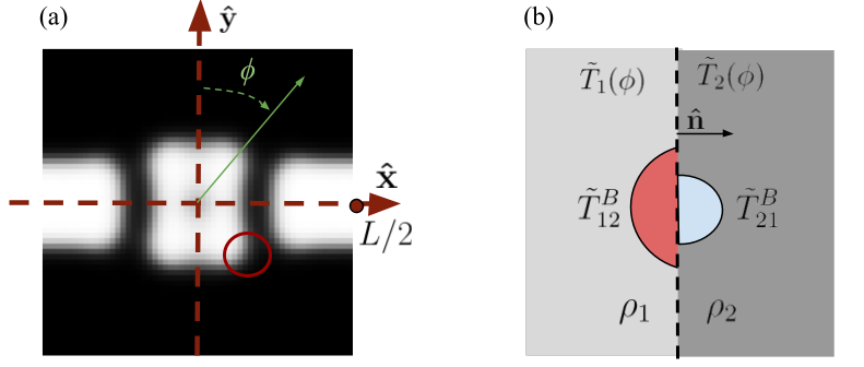
Figure 1: a) The simulation domain: a square centered in (0,0) and with side $L$. b) An example of interface between two regions with different densities, where the impinging, transmitted and isotropically reflected phonon temperatures are also shown.

It is straightforward to show that if either $\rho_{1}$ or $\rho_{2}$ is zero, then the RHS of Eq. 3 reduces to the hard-wall case. On the other side, if $\rho_{1}=\rho_{2}$, there will be no interface. To summarize, our parametrization does not relate the material density to a bulk-like property (such as the MFP from Ref. evgrafov2009topology), but rather to the amount of incoming flux. To distinguish this approach from traditional material interpolation methods, we name it the “Transmission Interpolation Model” (TIM). In passing, we note that transmission coefficients of the form $t^{\gamma}$, with $\gamma>1$ would also be a suitable interpolation approach. However, investigating this more general case is outside the scope of our work. Details on the angular discretization of TIM is reported in Sec. LABEL:sec:bte_solver.

4 The optimization pipeline

In this section, we outline the method for computing $\nabla_{\boldsymbol{\rho}}\bar{\kappa}$, which will be used in our optimization algorithm. We begin by noting that density-based topology optimization presents two major challenges: The emergence of rapidly oscillating “checkerboard” patterns that fail to converge with increasing spatial resolution; and gray ($0<\rho<1$) pixels, to which no physical material can be associated bendsoe2003topology.

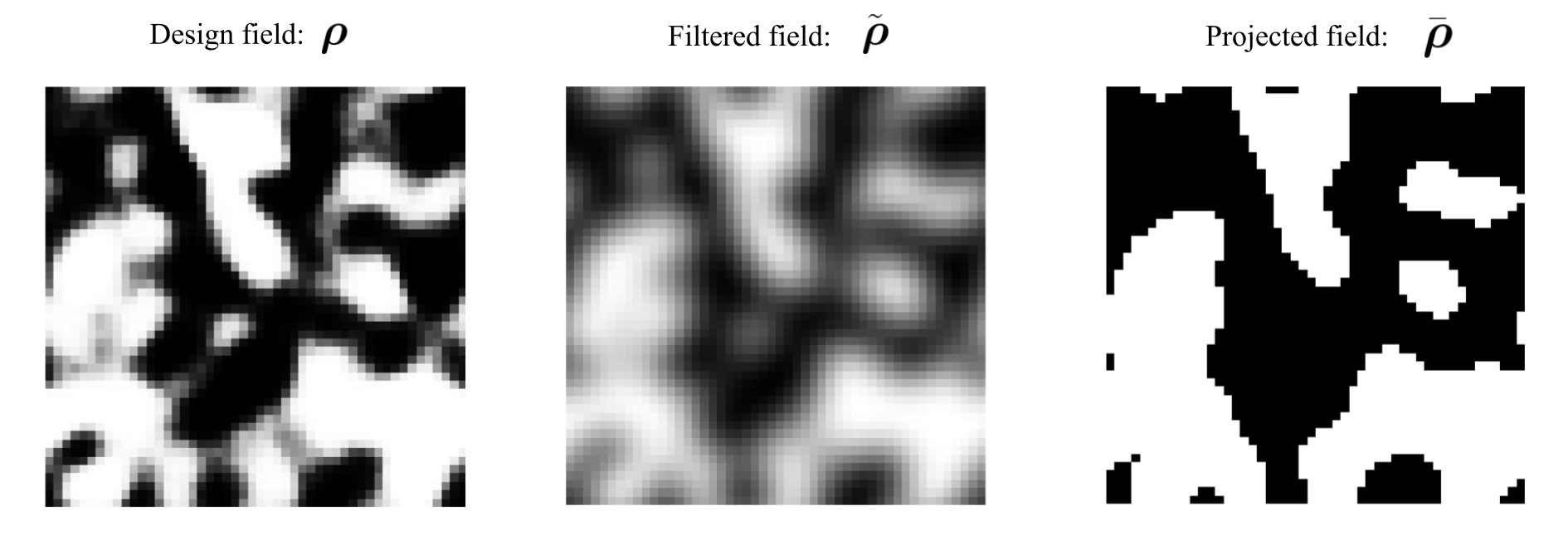
Figure 2: The design field $\boldsymbol{\rho}$ (in the left panel) is the optimization parameter. The filtered field $\tilde{\boldsymbol{\rho}}$, in the middle panel, is computed after the convolution with a conic filter, with Kernel defined in Eq. 10. The projected filter $\bar{\boldsymbol{\rho}}$, in the right panel, obtained with Eq. 11, is the input to the BTE.

These two issues are commonly resolved using filtering and thresholding, respectively sigmund2013topology. As shown in Fig. 2, given a design density $\boldsymbol{\rho}$ (for convenience, from now on, we will work with a discretized domain), we first filter it, $\tilde{\boldsymbol{\rho}}=\mathbf{w}*\boldsymbol{\rho}$, where, in this case, $\mathbf{w}$ is a conic filter with radius $R$,

$$w_{c}=\begin{cases}\frac{1}{a}\left(1-\frac{\mid\mathbf{r}_{c}\mid}{R}\right),&\mid\mathbf{r}\mid<R\\ 0,&\text{otherwise}.\end{cases}$$ (10)

In Eq. (10), $a$ is a normalization factor ($=\pi R^{2}/3$ in the continuum limit), $\mathbf{r}_{c}$ is the centroid of the grid point $c$, and $R$ is the radius of our filter. In this work, $R=L/10$. The thresholding, $\bar{\boldsymbol{\rho}}=f_{p}(\tilde{\boldsymbol{\rho}})$, is then carried out using the following function wang2011projection

$$\bar{\boldsymbol{\rho}}=\frac{\tanh{\beta\eta}+\tanh(\beta(\tilde{\boldsymbol{\rho}}-\eta))}{\tanh{\beta\eta}+\tanh(\beta(1-\eta))},$$ (11)

where $\eta$ and $\beta$ are threshold parameters. The resulting field, referred here as “projected” is, therefore, used directly by the BTE solver; in this work, we use $\eta=0.5$; the term $\beta$, on the other side, is increased during the optimization procedure hammond2021photonic, in order to guarantee a good degree of topology variability (especially early on in the optimization process) while ensuring a final binary structure. In this work, we start with $\beta=2$ and double it every 20 iterations, until convergence is reached.

Once the relationship $\bar{\boldsymbol{\rho}}(\boldsymbol{\rho})$ is implemented, we can use the chain rule

$$\frac{d\bar{\kappa}}{d\rho_{p}}=\sum_{\mu cp^{\prime}}\frac{\partial\bar{\kappa}}{\partial\tilde{T}_{\mu c}}\frac{\partial\tilde{T}_{\mu c}}{\partial\bar{\rho}_{p^{\prime}}}\frac{\partial\bar{\rho}_{p^{\prime}}}{\partial\rho_{p}}+\sum_{p^{\prime}}\frac{\partial\bar{\kappa}}{\partial\bar{\rho}_{p^{\prime}}}\frac{\partial\bar{\rho}_{p^{\prime}}}{\partial\rho_{p}},$$ (12)

which is evaluated using reverse-mode automatic differentiation, implemented in JAX jax2018github. Specifically, for $\partial\bar{\kappa}/\partial\bar{\rho}_{p}$ we use the adjoint method strang2007computational, which allows to compute such a gradient by solving the linear system

$$\sum_{\mu^{\prime}c^{\prime}}G_{\mu^{\prime}c^{\prime}}^{\mu c}\tilde{T}_{\mu^{\prime}c^{\prime}}^{\mathrm{adj}}=P^{\mathrm{adj}}_{\mu c},$$ (13)

with $P^{\mathrm{adj}}_{\mu c}$ defined in Sec. LABEL:sec:bte_solver. In practice, we use the relationship

$$\tilde{T}^{\mathrm{adj}}_{\mu c}=-\tilde{T}_{-\mu c},$$ (14)

derived in Sec. LABEL:sec:bte_solver. Therefore, the adjoint solution is computed by post-processing the solution of Eq. (5), achieving a significant boost in computational efficiency.

Furthermore, as $\nabla_{\bar{\boldsymbol{\rho}}}\bar{\kappa}$ is available at each iteration while solving the forward problem, we adopt an early termination criteria, based on $\bar{\kappa}$ and $\mid\nabla_{\bar{\boldsymbol{\rho}}}\bar{\kappa}\mid$. This approach extends Ref. amir2010efficient, where early termination strategies were based on the error on the objective function alone. The sensitivity of $\bar{\kappa}$ with respect to the projected density is provided through the custom vector-Jacobian-product $\mathrm{vJp}(a)=a\partial\bar{\kappa}/\partial\rho_{p}$. Lastly, we note that for the Fourier solver, the forward and adjoint solutions are related $\tilde{T}_{c}^{\mathrm{adj}}=-\tilde{T}_{c}$, as derived in Sec. LABEL:sec:fourier_solver Similarly to the BTE case, we use this relationship to avoid solving the adjoint problem.

5 Case I: Tailoring the Effective Thermal Conductivity Tensor

In this section, we show an example of how topology optimization may be employed to design a periodic material with a prescribed effective thermal conductivity tensor, $\tilde{\kappa}$, and with a porosity larger than $\tilde{\varphi}$. To this end, we define the objective function

$$g(\boldsymbol{\rho})=\mid\bar{\kappa}(\boldsymbol{\rho})-\tilde{\kappa}\mid_{\mathrm{Fro}}=\sqrt{\Delta\kappa_{xx}(\boldsymbol{\rho})^{2}+\Delta\kappa_{yy}(\boldsymbol{\rho})^{2}},$$ (15)

where $\text{.}\text{\_Fro}istheFrobeniusnorm,and\text{Δ}\text{κ}\text{\_ii(}\text{ρ}\text{) = }\overline{\text{κ}}\text{\_ii(}\text{ρ}\text{)-}\widetilde{\text{κ}}\text{\_ii}.Theeffectivethermalconductivitytensor,\text{(16)Equation 1616¯κ(ρ)=(¯κxx(ρ)00¯κyy(ρ)),}isevaluatedbysolvingEq.(\text{<a href="\#S2.E2" title="In 2 The 2D single-MFP BTE ‣ Inverse Design in Nanoscale Heat Transport via Interpolating Interfacial Phonon Transmission" class="ltx\_ref ltx\_font\_italic"><span class="ltx\_text ltx\_ref\_tag">2</span></a>}),foreachperturbationdirection,\text{after}filteringandprojecting.Thesensitivityoftheobjectivefunctionis\text{(17)Equation 1717∇ρg(ρ)=g(ρ)-1[Δκxx(ρ)∇¯ρ¯κxx(ρ)+Δκyy(ρ)∇ρ¯κyy(ρ)],}wheretheterms\text{∇\_}\text{ρ}\overline{\text{κ}}\text{\_ii(}\text{ρ}\text{)}arecomputedusingEq.\text{<a href="\#S4.E12" title="In 4 The optimization pipeline ‣ Inverse Design in Nanoscale Heat Transport via Interpolating Interfacial Phonon Transmission" class="ltx\_ref ltx\_font\_italic"><span class="ltx\_text ltx\_ref\_tag">12</span></a>}.Theabovediscussionallowsustolayouttheoptimizationalgorithm\text{(18)Equation 1818}where\text{N}isthenumberofpixels.Inthissection,thechosenporosityis\widetilde{\text{φ}}\text{= 0.25}.Astheoptimizer,weuseanopen-sourceimplementation\text{<cite class="ltx\_cite ltx\_citemacro\_cite"><span class="ltx\_ref ltx\_missing\_citation ltx\_ref\_self">johnson2014nlopt</span></cite>}ofthemethodofmovingasymptotes(MMA)\text{<cite class="ltx\_cite ltx\_citemacro\_cite"><span class="ltx\_ref ltx\_missing\_citation ltx\_ref\_self">svanberg2002class</span></cite>},whichconvergesglobally(i.e.itguaranteestofindalocalminimumfromeverystartingpoint).Asafirstexample,wechoose\widetilde{\text{κ}}\text{\_xx=}\widetilde{\text{κ}}\text{\_yy = 0.15}.Toensuremeshconvergenceonaparticularlocalminimum,weusethefollowingalgorithm:\text{1. Optimize a structure at a coarse resolution using a random configuration as the initial structure.2. Upsample the optimal structure by doubling the resolution.3. Optimize a structure using the configuration created in step 2 as the first guess. Note that the filter’s radius does not change in physical units, but doubles in pixel units.4. Repeat from step 2.}Figure\text{<span class="ltx\_ref ltx\_missing\_label ltx\_font\_italic ltx\_ref\_self">LABEL:fig:fig00</span>}illustratestheoptimizedstructuresforgridsizes\text{N=10×10, 20×20,40×40}and\text{80×80}.ForboththeFourierandBTEcases,ashapeconvergenceisachieved.Fortherestofthisstudyweadoptagridof\text{60×60},usingarandomconfigurationasafirstguess.AstrikingdifferencesbetweenthetwosolversisthatfortheBTEcasethepatterniscoarser.Infact,phononsizeeffectsareknowntobemoreeffectivethanmacroscopicreductionwiththesamegeometricconstraints\text{<cite class="ltx\_cite ltx\_citemacro\_cite"><span class="ltx\_ref ltx\_missing\_citation ltx\_ref\_self">sharvin1965possible</span></cite>}.Wenowturntothedesignananisotropicmaterial.Thermalanisotropymaybeinducedbyboundaryengineering,eventhoughthebasematerialisisotropic.Symmetry-breakingboundariesareeffectiveatallscales,althoughithasbeenshownnumericallythatnanostructuringmayenhanceanisotropywithrespecttothemacroscopiccounterpart\text{<cite class="ltx\_cite ltx\_citemacro\_cite"><span class="ltx\_ref ltx\_missing\_citation ltx\_ref\_self">romano2017thermal</span></cite>}.Inthisexample,wechoose\overline{\text{κ}}\text{\_xx = 0.3}and\overline{\text{κ}}\text{\_yy = 0.1},withtheresultinganisotropy\overline{\text{κ}}\text{\_xx/}\overline{\text{κ}}\text{\_yy= 3}.\text{Figure 3Figure 33Figure 33Theoptimizedstructuresusi}$