Spin supersolidity in nearly ideal easy-axis triangular quantum antiferromagnet Na₂BaCo(PO₄)₂

Abstract

Prototypical models and their material incarnations are cornerstones to the understanding of quantum magnetism. Here we show theoretically that the recently synthesized magnetic compound Na₂BaCo(PO₄)₂ (NBCP) is a rare, nearly ideal material realization of the $S=1/2$ triangular-lattice antiferromagnet with significant easy-axis spin exchange anisotropy. By combining the automatic parameter searching and tensor-network simulations, we establish a microscopic model description of this material with realistic model parameters, which can not only fit well the experimental thermodynamic data but also reproduce the measured magnetization curves without further adjustment of parameters. According to the established model, the NBCP hosts a spin supersolid state that breaks both the lattice translation symmetry and the spin rotational symmetry. Such a state is a spin analogue of the long-sought supersolid state, thought to exist in solid Helium and optical lattice systems, and share similar traits. The NBCP therefore represents an ideal material-based platform to explore the physics of supersolidity as well as its quantum and thermal melting.

Introduction
Quantum magnets are fertile ground for unconventional quantum phases and phase transitions. A prominent example is the $S=1/2$ triangular lattice antiferromagnet (TLAF). Crucial to the conception of the quantum spin liquid state [1], its inherent geometric frustration and strong quantum fluctuations give rise to exceedingly rich physics. In the presence of an external magnetic field, spin anisotropy, and/or spatial anisotropy, the system exhibits a cornucopia of magnetic orders and phase transitions [2, 3, 4]. In particular, introducing an easy-axis spin exchange anisotropy to the TLAF results in the spin supersolid [5, 6, 7, 8, 9, 10, 11] in zero magnetic field. Applying a magnetic field along the easy-axis drives the system through a sequence of quantum phase transitions by which the spin supersolidity disappears and then reemerges [12], whereas applying the field in the perpendicular direction yields distinct, even richer behaviors [13]. The $S=1/2$ easy-axis TLAF therefore constitutes a special platform for exploring intriguing quantum phases and quantum phase transitions.

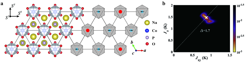
Fig. 1: Crystallographic structure of NBCP and fitting loss landscape. a Top view of the crystallographic structure of the NBCP. Each Co²⁺ ion carries an effective $S=1/2$ spin owing to the octahedral crystal environment and the spin-orbital coupling. The spins form a triangular network. Its magnetic ground state is a spin supersolid: the red (blue) circles represent the positive (negative) $S^{z}$ component, and the black arrows show the direction of the $S^{x,y}$ component. The crystallographic ${a}$-, ${b}$-, and ${c}$-axes and the spin frame $S^{x,y,z}$ are shown in the bottom right and the top left insets, respectively. b shows the projection of the fitting loss function onto the $J_{xy}$-$J_{z}$ plane (with $J_{\rm PD,\Gamma}$ fixed as zero), where brighter color represents less fitting loss and therefore better fit. The white cross marks the optimal parameter set, which corresponds to an $S=1/2$ TLAF with anisotropy parameter $\Delta=J_{z}/J_{xy}\simeq 1.7$ (dashed line).

Lately, a cobalt-based compound Na₂BaCo(PO₄)₂ (NBCP) has been brought to light [14, 15, 16, 17]. This material features an ideal triangular lattice of Co²⁺ ions, each carrying an effective $S=1/2$ spin owing to the crystal field environment and the significant spin-orbital coupling [18, 17] (Fig. 1a). Early thermodynamic measurements show that NBCP does not order down to $\sim 300$ mK with a large magnetic entropy ($\sim 2$ J mol^-1 K^-1) hidden below that temperature scale [14]. A later thermodynamic measurement reveals a specific heat peak at $\sim 150$ mK, which accounts for the missing entropy and points to a possible magnetic ordering in zero magnetic field [15]. However, the muon spin resonance ($\mu$SR) experiment finds strong dynamical fluctuation down to 80 mK [16] which may suggest a spin-liquid like state. The multitude of experimental results call for a theoretical assessment.

Previous works have attempted at establishing the spin exchange interactions in this compound. The authors in Ref. 15 suggest an exchange coupling $\sim 2$ K based on an analysis of the magnetic susceptibility data, which is an order of magnitude smaller than an earlier estimate of 21.4 K in Ref. 14. Meanwhile, a first-principle calculation suggests potentially significant Kitaev-type exchange interaction [17]. Despite these efforts, the precise spin Hamiltonian, its magnetic ground states, as well as the connection to experimental data, are yet to be established.

In this work, we show theoretically that NBCP can be well-described by a $S=1/2$ easy-axis TLAF with negligible perturbations. We establish the microscopic description of NBCP with realistic model parameters by fitting the model to intermediate- and high-temperature experimental thermal data. We expedite the fitting process by using the Bayesian optimization [19] equipped with an efficient quantum many-body thermodynamic solver — exponential tensor renormalization group (XTRG) [20, 21]. Our model is corroborated by reproducing quantitatively the experimental low-temperature magnetization curves by density matrix renormalization group (DMRG) [22] calculations. Furthermore, we are able to put the various experimental results into a coherent picture and connect them to the physics of the spin supersolid state. Therefore, the NBCP represents a rare material realization of this prototypical model system and thereby the spin supersolidity. The small exchange energy scale in this material ($\sim 1$ K) implies that the phases of the NBCP can be readily tuned by weak or moderate magnetic fields. Our results also highlight the strength of the many-body computation-based, experimental data-driven approach as a methodology for studying quantum magnets.

Results
Crystal symmetry and the spin-1/2 model. Figure 1a shows the lattice structure of NBCP and the crystallographic $a$-, $b$-, and $c$-axes. Due to the octahedral crystal field environment and the spin-orbital coupling, each Co²⁺ ion forms an effective $S=1/2$ doublet in the ground state, which is separated from higher energy multiplets by a gap of $\sim 71$ meV (see Supplementary Note 1). Super-super-exchange path through two intermediate oxygen ions produces exchange interactions between two nearest-neighbor (NN) spins, thereby connecting them into a triangular network (see density functional theory calculations in the Supplementary Note 2). Further neighbor spin exchange interactions are suppressed by the long distance. Meanwhile, the inter-layer exchange interactions are expected to be much smaller than the intra-layer couplings owing to the non-magnetic BaO layer separating the adjacent cobalt layers. Therefore, we model the NBCP in the experimentally relevant temperature window as a $S=1/2$ TLAF with dominant NN exchange interactions. This hypothesis will be justified a posteriori.

The crystal symmetry constrains the NN exchange interactions as follows [23]. The three-fold symmetry axis $\parallel c$ passing through each lattice site relates the exchange interactions on the 6 bonds emanating from that site. On a given bond, there is a 2-fold symmetry axis passing through that bond and a center of inversion. The former symmetry forbids certain components of the off-diagonal symmetric exchange interaction, whereas the latter forbids Dzyaloshinskii-Moriya interactions. We obtain

$$H_{ij}=\sum_{\alpha,\beta}J^{\alpha\beta}S_{i}^{\alpha}S_{j}^{\beta},$$ (1)

with

$$J^{\alpha\beta}=\begin{pmatrix}J_{xy}+2J_{\rm PD}\cos\varphi&-2J_{\rm PD}\sin\varphi&-J_{\Gamma}\sin\varphi\\ -2J_{\rm PD}\sin\varphi&J_{xy}-2J_{\rm PD}\cos\varphi&J_{\Gamma}\cos\varphi\\ -J_{\Gamma}\sin\varphi&J_{\Gamma}\cos\varphi&J_{z}\end{pmatrix},$$ (2)

where $i,j$ are a pair of neighboring lattice sites, and $\alpha,\beta$ label the spin $x,y,z$ components [24, 25, 26]. We choose the spin frame such that $x\parallel a$, $z\parallel c$. $\varphi=\{0,\frac{2\pi}{3},-\frac{2\pi}{3}\}$ for three different types of NN bonds parallel to $a$, $b$, and $-({a}+{b})$, respectively. $J_{xy}$, $J_{z}$, $J_{\Gamma}$, and $J_{\rm PD}$ are respectively the XY, Ising, off-diagonal symmetric, and pseudo-dipolar exchange couplings (see more details in Supplementary Note 3). The entire model parameter space is thus spanned by the four exchange constants, two Landé factors ($g_{ab}$ and $g_{c}$, for perpendicular and parallel to the $c$-axis, respectively), as well as two van Vleck paramagnetic susceptibilities ($\chi_{ab}^{\rm vv},\chi_{c}^{\rm vv}$), all of which are taken to be constants in the experimentally relevant temperature/magnetic field window.

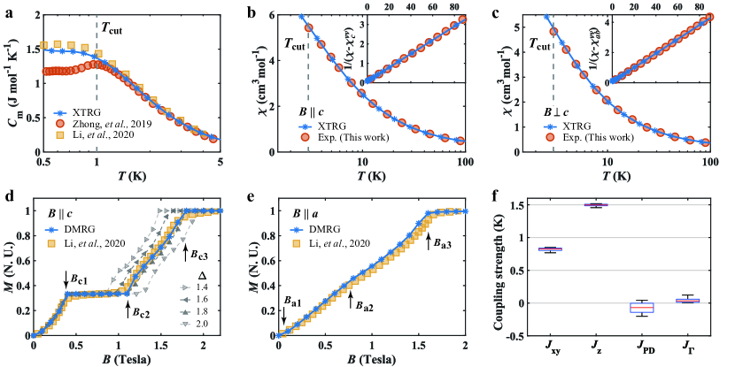
Fig. 2: Thermodynamic data fittings, magnetization curves, and the optimal model parameters. a shows the magnetic specific heat $C_{\rm m}$ of the NBCP as a function of temperature $T$, reported by two independent measurements (Zhong et al. 2019 [14] and Li et al. 2020 [15]) as well as the best fit. The gray dashed line marks $T_{\rm cut}$. The XTRG fitting is performed for experimental data at $T>T_{\mathrm{cut}}$. b, c show respectively parallel and perpendicular to the $c$-axis magnetic susceptibilities with the experimental data measured in this work (see Methods) and the best fit. d, e show the magnetization as a function of the magnetic field in the ${c}$ and ${a}$ directions, respectively. The experimental data were obtained from Li et al. 2020 [15] with the van Vleck paramagnetic contributions subtracted off. The model prediction is obtained from DMRG, which agrees quantitatively with experiment. The grey lines show magnetization curves obtained from models with various anisotropy parameters $\Delta$, with $J_{xy}$ tuned to the optimal value. f shows the standard box plot of the optimal parameters, with the red line indicating the median value, the top(bottom) edge of the box representing the upper(lower) quartile of the best 20 model parameter sets found in 450 Bayesian optimization runs.

Determination of the model parameters. We determine the model parameters in Eq. (1) by fitting the experimental magnetic specific heat ($C_{\rm m}$) and magnetic susceptibility ($\chi$) data at temperature $T\geq T_{\rm cut}$, where $T_{\rm cut}=1$ K for $C_{\rm m}$ and 3 K for $\chi$. Note the magnetic susceptibilities are remeasured in this work with high quality samples. For each trial parameter set, we compute the same thermodynamic quantities from the model by using the XTRG solver [27, 21]. We search for the parameter set that minimizes the total loss function through an unbiased and efficient Bayesian optimization process [19]. See Methods for more details.

We set the cutoff temperature $T_{\mathrm{cut}}$ based on the following considerations. The experimental data from independent measurements agree with each other at $T>T_{\mathrm{cut}}$, and our XTRG solver does not exhibit significant finite-size effects above $T_{\mathrm{cut}}$. Meanwhile, the $T_{\mathrm{cut}}$ has to be less than or comparable with the characteristic energy scale of the material. These constraints fix $T_{\mathrm{cut}}$ to our present choices.

The searching process yields the following optimal parameter set: $J_{xy}=0.88$ K, $J_{z}=1.48$ K, and $J_{\Gamma,\rm PD}$ are negligible. The Landé factors $g_{ab}=4.24$, and $g_{c}=4.89$. The van Vleck susceptibilities $\chi^{\rm vv}_{ab}=0.149$ cm³ mol^-1 and $\chi^{\rm vv}_{c}=0.186$ cm³ mol^-1. To ensure that the algorithm does converge to the global minimum, we project the loss function onto the $(J_{xy},J_{z})$ plane in Fig. 1b, where, for fixing values of $J_{xy},J_{z}$, the loss function is minimized over the remaining parameters. The fitting landscape reveals a single minimum. The estimated value of exchange parameters and their bounds of uncertainty are shown in Fig. 2f.

The small uncertainties in $J_{xy}$ and $J_{z}$, as well as the small loss, indicate that the experimental data are well captured by our parameters. Indeed, Fig. 2a-c show respectively the specific heat and the magnetic susceptibility as functions of temperature. We find excellent agreement between the model calculations and the experiments within the fitting temperature range $T\geq T_{\rm cut}$. Reassuringly, the Landé factors obtained by us are in excellent agreement with the latest electron-spin resonance measurement ($g_{ab}=4.24$ and $g_{c}=4.83$) [17]. We have also calculated the magnetic specific heat $C_{\rm m}$ in non-zero magnetic fields and find good agreement with the experiments whenever the two independent measurements [14, 15] mutually agree (Supplementary Note 4). Note in Fig. 2a the two experimental data sets of specific heat differ at $T<T_{\rm cut}$. Our model’s behavior below $T_{\rm cut}$ is in agreement with one of them. The discrepancy in the experimental data calls for further investigation.

Our model parameters pinpoint to an almost ideal $S=1/2$ TLAF with significant easy-axis anisotropy $\Delta=J_{z}/J_{xy}\approx 1.68$. In particular, the negligible off-diagonal exchange interactions imply that the NBCP features an approximate U(1) spin rotational symmetry with respect to $c$ axis. As a result, the magnetization curve with field $B\parallel c$ in Fig. 2d has a couple of idiosyncratic features: It shows a $1/3$-magnetization plateau in an intermediate field range $[B_{c1},B_{c2}]$, and another fully magnetized plateau above the saturation field $B_{c3}$. As an independent estimate of $\Delta$, we note the semi-classical analysis shows that $B_{c2}/B_{c1}=\Delta-1/2+\sqrt{\Delta^{2}+\Delta-7/4}$ and $B_{c3}/B_{c1}=2\Delta+1$ (Supplementary Note 5). Using the experimental values $B_{c1}\approx 0.35$ T and $B_{c3}\approx 1.62$ T [15], we estimate $\Delta\approx 1.81$, which is consistent with the Bayesian search result. Meanwhile, using these numbers, we can estimate $B_{c2}\approx 1.10$ T, which is fairly close to the experimental value of $1.16$ T [15].

As a corroboration of our model, we perform DMRG calculations of the zero-temperature magnetization curves and find quantitative agreement with the experimental results (Fig. 2d, e). With no further adjustment of the parameters, the model can not only produce the correct transition fields but also the details of the magnetization curve between the transitions. We find that the magnetization curve $\parallel c$ is a sensitive diagnostic for the anisotropy parameter $\Delta$. The agreement between the model and the experiments is quickly lost when $\Delta$ deviates slightly from the optimal value in Fig. 2d.

Taken together, the broad agreements between the semi-classical estimates, the quantum many-body calculations, and experimental data strongly support the $S=1/2$ easy-axis TLAF as an effective model description for the NBCP.

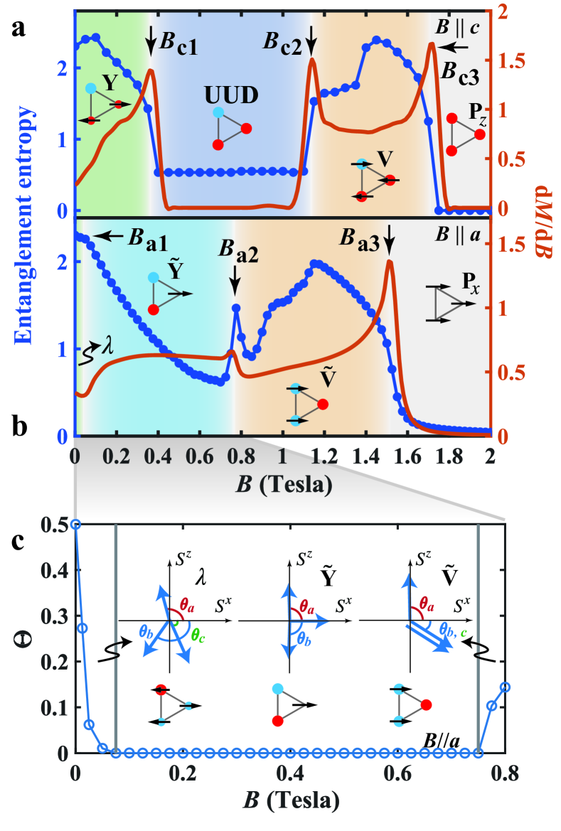
Fig. 3: Zero-temperature phase diagrams under in- and out-of-plane fields. a shows the entanglement entropy and differential magnetic susceptibility $dM/dB$ as functions of field $B$ in the ${c}$ direction. The Y, UUD, V, and P_z phases are shaded in different colors. $B_{c1,c2,c3}$ are the three critical fields separating these phases. The corresponding spin configurations are also shown. Red (blue) circles represent the positive (negative) $S^{z}$ component. Black arrows show the direction of the in-plane ($S^{x,y}$) component. b is similar to a but for field $B\parallel a$. The $\lambda$ phase, $\widetilde{\mathrm{Y}}$ phase, $\tilde{\rm V}$ phase, and P_x phase are separated by three critical fields $B_{a1,a2,a3}$. c is a zoom-in of b, showing the side view of the spin configurations, as well as the evolution of the order parameter $\Theta$ as a function of the field (see main text for definition).

Field-tuning of the spin supersolid state. The $S=1/2$ easy-axis TLAF exhibits a sequence of magnetic phases and quantum phase transitions driven by magnetic fields [12, 28, 29]. The experimentally measured differential susceptibilities ($dM/dB$) show a few anomalies when the field is $\parallel c$ and $\parallel a$ and are attributed to quantum phase transitions [15]. Here, we clarify the nature of the magnetic orders of NBCP based on the $S=1/2$ easy-axis TLAF model.

Figure 3a shows the theoretical zero-temperature phase diagram of our model in field $\parallel c$, obtained from DMRG calculations. The system goes through successively the Y, Up-Up-Down (UUD), V, and the polarized (P_z) phases with increasing field. These phases are separated by three critical fields $B_{c1,c2,c3}$ = 0.36 T, 1.14 T, 1.71 T discussed in the previous section, which are manifested as peaks in $dM/dB$. The Y phase, as well as the V phase, spontaneously break both the lattice translation symmetry and the U(1) symmetry, thereby constituting the supersolid state analogous to that of the Bose atoms. The UUD phase, on the other hand, restores the U(1) symmetry but breaks the lattice translation symmetry. This state is analogous to a Bose Mott insulator state. The magnetic plateau associated with the UUD state reflects the incompressibility of the Mott insulator.

Fig. 4: Finite-temperature phase diagram of the NBCP under magnetic fields $\parallel c$. a shows $C_{\text{m}}/T$, calculated from XTRG, as a function of temperature $T$ and magnetic field $\parallel c$. The open squares mark the peaks of the experimental $C_{\text{m}}/T$ data (Li et al. 2020 [15]). b shows $C_{\rm m}/T$ under zero field, and the magnetic entropy $S_{\rm m}$, as functions of temperature. The experimental $S_{\rm m}$ data are obtained by integrating numerically the $C_{\rm m}/T$ data. The experimental entropy curve is shifted by $0.55~{}\text{J}~{}\text{mol}^{-1}~{}\text{K}^{-1}$ to match the saturation value $R\ln(2)$ at sufficiently high temperature. c shows the temperature-field phase diagram constructed from the classical Monte Carlo (MC) simulation. The blue triangles mark the three-state Potts transitions determined by using the Binder cumulants. Red solid circles mark the BKT transitions determined from the spin stiffness (see Methods). The zero field BKT transition temperatures are reported by Ref. [30]. The red solid line along the vertical axis under zero field indicates the regime with algebraic spin correlation in the $S^{z}$ spin component. d shows the specific heat as a function of temperature for various representative magnetic field $\parallel c$, obtained from the classical MC simulation.

The situation is yet more intricate when the field $\parallel a$. DMRG calculations show that the system goes through the $\lambda$, $\tilde{\rm Y}$, $\tilde{\rm V}$ (see Fig. 3c for an illustration), and the quasi-polarized ${\rm P}_{x}$ phases, which are separated by three critical fields $B_{a1}$ = 0.075 T, $B_{a2}$ = 0.75 T, and $B_{a3}$ = 1.51 T. The presence of a field $\parallel a$ breaks the U(1)-rotational symmetry with respect to the $S^{z}$ axis but preserves the $\pi$-rotational ($Z_{2}$) symmetry with respect to the $S^{x}$ axis. The $\lambda$ phase, where the spins sitting on three magnetic sublattices form the greek letter “$\lambda$”, spontaneously breaks both the $Z_{2}$ symmetry and the lattice translation symmetry. The $Z_{2}$ symmetry is restored in the $\tilde{\rm Y}$ phase, and spontaneously broken again in the $\tilde{\rm V}$ phase.

Comparing to the field-induced transitions in $B\parallel c$ case, the transitions at $B_{a1,a2}$ show much weaker anomalies in $dM/dB$ when $B\parallel{a}$. Numerically, we detect these two transitions using an order parameter $\Theta=\frac{1}{\pi}|(\theta_{a}-\theta_{b}-\theta_{c})|$, where $\theta_{a,b,c}$ measure the angle between the spin moments on three sublattice and the $S^{x}$ axis. $\Theta=0$ when the $Z_{2}$ symmetry is respected and $\Theta\neq 0$ when it is broken. Figure. 3c shows $\Theta$ as a function of field, from which we can delineate the boundaries between $\lambda$, $\tilde{\rm Y}$, and $\tilde{\rm V}$ phases, with the critical fields $B_{a1}\approx 0.07$ T and $B_{a2}\approx 0.75$ T. The small value of $B_{a1}$ implies it could be easily missed in experiments. Meanwhile, the weak anomalies in $dM/dB$ associated with $B_{a1,a2}$ make them difficult to detect in thermodynamic measurements. We note that $dM/dB$ shows a broad peak in the $\tilde{\rm Y}$ phase at $\sim$ 0.4-0.5 T [15]. This peak appears in the experimental data and was previously interpreted as a transition. The true transitions ($B_{a1,a2}$) are in fact above and/or below the said peak. We also note that, despite of the weak anomaly observed numerically at $B_{a2}$, the quantum phase transition there is likely of first-order from symmetry analysis: the $\tilde{\rm Y}$ and $\tilde{\rm V}$ phases both have a 6-fold ground-state degeneracy and they have incompatible symmetry breaking; thus the transition cannot be continuous according to Landau’s paradigm.

Strong spin fluctuations and phase diagram at finite temperature. Having established the zero-temperature phase diagram of the NBCP, we now move on to its physics at finite temperature. Figure 4a shows the contour plot of $C_{\rm m}/T$ as a function of temperature and field $B\parallel c$. In the temperature window accessible to the XTRG, we find a broad peak near zero field, which moves to higher temperature and becomes sharper as field increases. These features are in qualitative agreement with the experimental findings.

Figure 4b shows a cross-section of the contour plot at zero field. The model produces a peak in $C_{\rm m}/T$ at $\approx 150$ mK, which is in excellent agreement with the experimental data from Ref. [15]. Note this temperature is well below the temperature window (above $T_{\rm cut}$) used for fitting, the difference between theory and experiment at very low temperatures may be ascribed to the finite-size effect inherent in the XTRG calculations (see Methods). The magnetic entropy also shows quantitative agreement with the experimental data. In particular, there is still a considerable amount of magnetic entropy to be released at 300 mK (and even down to 150 mK). The missing entropy at 300 mK reported in Ref. [14] can be ascribed to the small spin interaction energy scale and high degrees of frustration in the NBCP.

To understand the finite-temperature phase diagram of the NBCP, we perform a Monte Carlo (MC) simulation of the classical TLAF model with appropriate rescaling of temperature and magnetic field [31, 30, 32, 33]. This approximation is amount to neglecting fluctuations in the imaginary time direction in the coherent-state path integral of the $S=1/2$ TLAF. As the finite-temperature phase transitions are driven by thermal fluctuations, we expect that the salient features produced by the classical MC simulations are robust. Meanwhile, the MC simulation allows for accessing much larger system sizes and lower temperatures comparing to the XTRG for quantum model simulations.

The physics of the classical TLAF model is well documented; here, we focus on the features that can be directly compared with available experimental data. Figure. 4c shows the MC-constructed $T$-$B$ phase diagram with $B\parallel{c}$. Figure. 4d shows the specific heat as a function of temperature for various representative fields. The phase diagram shows a broad dome of UUD phase, beneath which lie the Y phase at low field and the V phase at high field. The UUD phase and the paramagnetic phase are separated by a transition of three-state Potts universality; the Y and V phases and the UUD phase are seperated by the Berezinskii-Kosterlitz-Thoueless (BKT) transitions. Note the MC simulation may seem to suggest the onset of the V phase precedes that of the UUD phase at high field; this is an finite-size effect. On symmetry ground, we expect that the onset of the UUD phase either precedes that of the V phase through two continuous transitions, or the system enters the V phase directly through a first-order transition.

At zero field, the specific heat shows two broad peaks, which are related to the two BKT transitions accompanying the onset of the algebraic long-range order in $S^{z}$ and $S^{x}$ components, respectively [31, 30]. The experimentally observed specific heat peak $\sim 150$ mK may be related to the higher-temperature BKT transition; the lower-temperature BKT transition (around 54 mK as estimated by classical MC simulations) is yet to be detected as they lie below the temperature window probed by the previous experiments. The strong dynamical spin fluctuations found in $\mu$SR experiment at 80 mK is naturally attributed to the algebraic long-range order in the $S^{z}$ component. Note there exists arguments for a third BKT transition [32] although it is not observed in classical MC simulations [30].

When the magnetic field is switched on, the specific heat shows a sharp peak signaling the three-state Potts transition from the high temperature paramagnetic phase to the UUD phase, corresponding to onset of the long-range order in the $S^{z}$ component. This is consistent with the experimentally observed sharp specific heat peak at finite fields [15]. At lower temperature, the specific heat shows a much weaker peak related to the BKT transition into either the Y phase or the V phase, corresponding to the onset of the algebraic long-range order in $S^{x}$. The lower temperature BKT transitions are yet to be detected by experiments.

Discussion
The supersolid, a spatially ordered system that exhibits superfluid behavior, is a long-pursued quantum state of matter. The question of whether such a fascinating phase of matter exists in nature has spurred intense research activity, and the search for supersolidity has become a multidisciplinary endeavour [34, 35, 36, 37, 38, 39]. The early claim of observation in He-4 [34] turned out to be an experimental artifact [35]. Nevertheless, it has inspired new lines of research in ultracold quantum gases [36, 37, 38, 39]. Meanwhile, it has been proposed theoretically that the ultracold Bose atoms in a triangular optical lattice can host a supersolid state [5, 6, 7, 8]. Yet, the realization of such a proposal has not been reported up to date.

An equivalent, yet microscopically different route to the triangular lattice supersolidity is via the easy-axis $S=1/2$ TLAF magnet. The spin up/down state of a magnetic ion can be viewed as the occupied/empty state of the lattice site by a Bose atom, and the spin rotational symmetry with respect to the easy axis is mapped to the U(1) phase rotation symmetry. By virtue of this mapping, the spin ground state in the easy-axis TLAF, which spontaneously breaks both lattice translation symmetry and spin rotational symmetry, is equivalent to the supersolid state of Bose atoms.

Despite its simple setting, ideal $S=1/2$ TLAF has rarely been found in real materials. Although TLAFs with higher spin ($S>1/2$) are known [3], $S=1/2$ systems with equilateral triangular lattice geometry, such as Ba₃CoSb₂O₉ [40, 41, 42, 43, 44, 45, 46, 47] and Ba₈CoNb₆O₂₄ [48, 49], were synthesized and characterized not until recently. The former shows easy-plane anisotropy [28, 47], whereas the latter material is thought to be nearly spin isotropic [48, 49, 50]. To the best of our knowledge, ideal $S=1/2$ easy-axis TLAFs are yet to be found. In this work, we show that the NBCP is an almost ideal material realization of such an $S=1/2$ easy-axis TLAF with the anisotropy parameter $\Delta\approx 1.7$.

Our model arranges the various pieces of available experimental data into a coherent picture by connecting them to the rich physics of the TLAF model. It permits a quantitative fit of the thermodynamic data, including specific heat $C_{\rm m}$ and magnetic susceptibility $\chi$ down to intermediate and even low temperatures. In particular, we obtain the $C_{\rm m}/T$ peak at around 150 mK observed in experiments [15], which we associate to the BKT transition. Furthermore, we are able to accurately reproduce the spin state transition fields observed in previous AC susceptibility measurements along both $a$ and $c$ axes and clarify their nature.

The obtained spin exchange interactions are on similar orders of magnitude as previous estimation based on the Curie-Weiss fitting of the magnetic susceptibility [15] and first-principle calculation [17]. However, the first-principle calculation suggests a significant Kitaev-type exchange interaction (in a rotated spin frame) [17], whereas our model, being directly fitted from the experimental data, possesses a nearly ideal U(1) symmetry and negligible Kitaev-type interaction (see more discussions in Supplementary Note 3). The nearly ideal U(1) symmetry in this material is indicated by the well-quantized magnetization plateau (Fig. 2d), which would be absent without the U(1) symmetry.

In our fitting procedure, we have omitted at the outset all further-neighbor exchange interactions on the ground that their magnitude must be suppressed by the large distance between further-neighbor Co²⁺ ions. This can be verified by including in the model a second-neighbor spin-isotropic exchange interaction $J_{2}$. To verify it, we have performed addtional 400 Bayesian iterations and find $J_{2}$ with the median value $\sim 0.1$ K amongst the best 20 parameter sets, which are negligibly small. We thus conclude the obtained optimal parameters in the simulations are robust.

Despite the essential challenge in the first-principle calculations of the strongly correlated materials, we may nevertheless employ the density functional theory (DFT) + U approach to justify certain aspects of the microscopic spin model that are accessible to this approach. First of all, we find the charge density distributions of 3$d$ electrons of Co²⁺ ions are well separated from one triangular plane to another (see Supplementary Note 2), which ensures two-dimensionality of the compound. Moreover, the in-plane charge density distribution reveals clearly a super-super-exchange path between the two NN Co²⁺ ions. We construct the Wannier functions of $d$-orbitals of Co²⁺ ions and extract the hopping amplitude $t$ between two NN Co²⁺ ions. From the second-order perturbation theory in $t/U$, the NN exchange coupling can be estimated to be on the order of $2\sim 3$ K for moderate and typical $U_{\rm eff}=4\sim 6$ eV in this Co-based compound [17], which is consistent with the energy scales of the spin model.

The accurate model for the NBCP also points to future directions for the experimentalists to explore. The model hosts a very rich phase diagram in both temperature and magnetic field, which are yet to be fully uncovered by experiments. In particular, the model shows a second BKT transition at $\sim 50$ mK in zero field; in finite field $B\parallel a$, the model shows two subtle transitions at $B_{a1}\approx 0.07$ T and $B_{a2}\approx 0.75$ T. These transitions may be detected by nuclear magnetic resonance [51], magneto-torque measurements [52], and magnetocaloric measurements [53, 54, 55]. Neutron scattering experiments can also be employed to detect the simultaneous breaking of discrete lattice symmetry and spin U(1) rotational symmetry, as well as the behaviors of spin stiffness, so as to observe spin supersolidity in this triangular quantum magnet. On the theory front, while the $S=1/2$ easy-axis TLAF and its classical counterpart share similar features in their finite-temperature phase diagrams, it was realized early on that the quantum model also possess peculiar traits that are not fully captured by the classical model [32]. Clarifying these subtleties in the context of NBCP would also presents an interesting problem for the future.

Methods
Exponential tensor renormalization group. The thermodynamic quantities including the magnetic specific heat $C_{\rm m}$, and magnetic susceptibility $\chi$ can be computed with the exponential tensor renormalization group (XTRG) method [27, 21]. In practice, we perform XTRG calculations on the Y-type cylinders with width $W=6$ and length up to $L=9$ (denoted as YC6$\times$9, see Supplementary Note 4), and retain up to $D=400$ states with truncation errors $\epsilon\lesssim 1\times 10^{-4}$ (down to 1 K) and $\lesssim 1\times 10^{-3}$ (down to about 100 mK). The XTRG truncation provides faithful estimate of error in the computed free energy, and the small $\epsilon$ value thus guarantee high accuracy of computed thermal data down to low temperature.

The XTRG simulations start from the initial density matrix $\rho_{0}(\tau)$ at a very high temperature $T\equiv 1/\tau$ (with the inverse temperature $\tau\ll 1$), represented in a matrix product operator (MPO) form [56]. The series of density matrices $\rho_{n}(2^{n}\tau)$ ($n\geq 1$) at lower temperatures are obtained by iteratively multiplying and compressing the MPOs $\rho_{n}=\rho_{n-1}\cdot\rho_{n-1}$. As a powerful thermodynamic solver, XTRG has been successfully applied in solving triangular-lattice spin models [50] and related compounds [57, 51], Kitaev model [58] and materials [59], correlated fermions in ultra-cold quantum gas [60], and even moiré quantum materials [61].

Automatic parameter searching. By combining the thermodynamic solver XTRG and efficient Bayesian optimization approach, the optimal model parameters can be determined automatically via minimizing the fitting loss function between the experimental and simulated data, i.e.,

$$\mathcal{L}(\mathbf{x})=\frac{1}{N_{\alpha}}\sum_{\alpha}\frac{(O^{\mathrm{exp}}_{\alpha}-O^{\rm sim,\mathbf{x}}_{\alpha})^{2}}{(O^{\rm exp}_{\alpha})^{2}}.$$ (3)

$O^{\rm exp}_{\alpha}$ and $O^{\rm sim,\mathbf{x}}_{\alpha}$ are respectively the experimental and simulated quantities with given model parameters $\mathbf{x}\equiv\{J_{xy},J_{z},J_{\rm PD},J_{\Gamma},g_{ab,c},\chi^{\rm vv}_{ab,c}\}$. The index $\alpha$ labels different physical quantities, e.g., magnetic specific heat and susceptibilities, and $N_{\alpha}$ counts the number of data points in $O_{\alpha}$. The optimization of $\mathcal{L}$ over the parameter space spanned by $\{J_{xy},J_{z},J_{\rm PD},J_{\Gamma}\}$ is conducted via the Bayesian optimization [19]. The Landé factor $g_{ab,c}$ and the Van Vleck paramagnetic susceptibilities $\chi^{\rm vv}_{ab,c}$ are optimized via the Nelder-Mead algorithm for each fixing $\{J_{xy},J_{z},J_{\rm PD},J_{\Gamma}\}$. In practice, we perform the automatic parameter searching using the package QMagen developed by some of the authors [19, 62], and the results shown in the main text are obtained via over 450 Bayesian iterations. After that, we introduce an additional parameter, the next-nearest-neighbor Heisenberg term $J_{2}$, and perform another 400 searching iterations. We find $J_{2}$ is indeed negligibly small and the obtained optimal parameters are robust.

Density matrix renormalization group. The ground state magnetization curves of the easy-axis TLAF model for NBCP are computed by the density matrix renormalization group (DMRG) method [22], which is a powerful variational algorithm based on the matrix product state ansatz. The DMRG simulations are performed on YC6$\times$15 lattice, and we retain bond dimension up to $D=1024$ with truncation error $\epsilon<3\times 10^{-5}$, which guarantees well converged DMRG data.

Classical Monte Carlo simulations. We replace the $S=1/2$ operators by classical vectors, $S^{x,y,z}_{i}\to S\hat{n}_{i}$, where $\hat{n}_{i}$ is a unit vector, and $S=1/2$ is the spin quantum number. We use the standard Metropolis algorithm with single spin update. The largest system size is 48$\times$48. We compute the Binder ratio associated with the UUD-phase order parameter $\psi=m_{1}+m_{2}\exp(i2\pi/3)+m_{3}\exp(-i2\pi/3)$, where $m_{1,2,3}$ are respectively the $S^{z}$-axis magnetization of the three sublattices, as well as the in-plane spin stiffness $\rho$ [30]. We locate the three-state Potts transition by examining the crossing of the Binder ratio, and the BKT transition by the criterion $\rho_{c}=(2/\pi)T_{c}$.

In the simulations, we use the natural unit in the calculation and thus the following process is required for comparing the model calculation results in the natural unit to experimental data in SI units:

• The value of temperature $T$ in natural unit should be multiplied by a factor of $J_{xy}$, and change it thus to the unit of Kelvin, where $J_{xy}=0.88~{}{\rm K}$ is taken as the energy scale in the calculation.

• Multiply the value of specific heat $C_{\rm m}$ in natural unit by a factor of $R$, i.e., the ideal gas constant, and change it to the unit of J mol^-1 K^-1.

• Multiply the magnetic field $h$ in natural unit by a factor of ${J_{xy}k_{B}}/{(g_{z}\mu_{B})}$ and it is now in unit of Tesla, where $g_{z}$ is the Landé factor along $S_{z}$ direction and $\mu_{B}$ the Bohr magneton.

Sample preparation and susceptibility measurements. Single crystals of Na₂BaCo(PO₄)₂ were prepared by the flux method starting from Na₂CO₃ (99.9%), BaCO₃ (99.95%), CoO (99.9%), (NH₄)₂HPO₄ (99.5%), and NaCl (99%), mixed in the ratio 2:1:1:4:5. Details of the heating procedure were given in Ref. [14]. The flux generated after the reaction is removed by ultrasonic washing. The anisotropic magnetic susceptibility measurements in this work were performed using a SQUID magnetometer (Quantum Design MPMS 3). The magnetic susceptibility as a function of temperature was measured in zero field cooled runs. During the measurements, magnetic field of 0.1 T was applied either parallel or perpendicular to the ${c}$ axis. In the latter (in-plane) measurements, no anisotropy is observed in the obtained susceptibility data.

Data availability
The data that support the findings of this study are available from the corresponding author upon reasonable request.

Code availability
All numerical codes in this paper are available upon request to the authors.

 
Acknowledgements

W.L. and Y.G. are indebted to Tao Shi for stimulating discussions, W.L. would also thank Xue-Feng Sun and Jie Ma for valuable discussions on the experiments. This work was supported by the National Natural Science Foundation of China (Grant Nos. 12222412, 11834014, 11874115, 11974036, 11974396, 12047503, and 12174068), the Strategic Priority Research Program of the Chinese Academy of Sciences (Grant No. XDB33020300), and CAS Project for Young Scientists in Basic Research (Grant Nos. YSBR-057 and YSBR-059). We thank the HPC-ITP for the technical support and generous allocation of CPU time.

 
Competing interests
The authors declare no competing interests.

 
Author contributions
W.L., Y.Q., and Y.W. initiated this work. Y.G. and H.L. performed XTRG and DMRG calculations of the TLAF model. Y.W. conducted the symmetry and semi-classical analyses. X.T.Z., F.Y., and X.L.S. did the CEF point charge model analysis and DFT calculations. Y.C.F. undertook the MC simulations. R.Z. prepared the sample and performed the susceptibility measurements. All authors contributed to the analysis of the results and the preparation of the draft. Y.W. and W.L. supervised the project.

 
Additional information
Supplementary Information is available in the online version of the paper.
Correspondence and requests for materials should be addressed to Y.W. or W.L.

Supplementary Note 1 Crystal electric field calculations of Na₂BaCo(PO₄)₂

According to the Hund’s rule, the lowest-energy electron structure of a free Co²⁺ ion is ${}^{4}F(L=3,S=3/2)$ with the high-spin state. We consider the energy spectrum of ${}^{4}F$ state under CEF and spin-orbit coupling with the effective Hamiltonian

$$H=H_{\rm SOC}+H_{\rm CEF}=\lambda S\cdot L+\sum_{n,m}B_{n}^{m}O_{n}^{m},$$ (1)

where $S$ is the spin angular momentum, $L$ is the orbital angular momentum, and $O_{n}^{m}$’s are the Stevens’ operators with multiplicative CEF parameters $B_{n}^{m}$. Due to the time-reversal symmetry constraint, the operator degree $n$ is required to be even, and $m$ is the operator order which satisfies $-n\leq m\leq n$. It is necessary to treat both CEF and spin-orbit coupling non-perturbatively, namely the intermediate coupling scheme, where $H_{\rm CEF}$ acts only on the orbital angular momentum $L$ [63].

Supplementary Tabel 1: The two lowest CEF states in the Kramers doublet.

J = 9/2
$L_{z}$	-3		-2			-1			0		1			2			3
$S_{z}$	-1/2	1/2	-3/2	-1/2	3/2	-3/2	1/2	3/2	-1/2	1/2	-3/2	-1/2	3/2	-3/2	1/2	3/2	-1/2	1/2
1	-0.41	-0.02	-0.71	-0.03	-0.04	-0.01	-0.19	-0.02	-0.32	-0.04	-0.21	-0.02	0.10	-0.01	0.29	0.08	0.19	0.05
2	0.05	-0.19	0.08	-0.29	0.01	-0.10	0.02	-0.21	0.04	-0.32	0.02	-0.19	-0.01	-0.05	-0.03	0.71	-0.02	0.41

Constructing a point charge model directly from Na₂BaCo(PO₄)₂ structure and perform the calculations with the open-source package PyCrystalField [64], we obtain the three CEF constants $B_{2}^{0}=-3.75$ meV, $B_{4}^{0}=0.45$ meV, and $B_{4}^{3}=11.51$ meV. Considering the spin-orbit coupling constant $\lambda=-65.34$ meV from experiments [65, 66], the obtained CEF levels are shown in Supplementary Figure 1, where the two lowest levels constitute a Kramers doublet, i.e., the effective spin-1/2 degree of freedom in the spin-orbit magnet. We further show the wavefuctions of the two CEF states with coefficients of each $(L_{z},S_{z})$ components listed in Supplementary Table 1, where the components with large $J_{z}$, like $\pm 9/2$, $\pm 7/2$, etc., have relatively large weights. This suggests an easy-axis anisotropy of the compound from the single-ion physics. Meanwhile, the CEF splitting between the lowest Kramers doublet to the higher levels is about 900 K ($\sim$ 71 meV), rendering clearly an effective spin-1/2 magnet at relevant temperature in the study of spin supersolidity in this work.

Supplementary Figure 1: The electronic state of Co²⁺ ion in the compound Na₂BaCo(PO₄)₂, where the two degenerate lowest levels form an effective spin-1/2 doublet.

Supplementary Note 2 DFT+U calculations of Na₂BaCo(PO₄)₂

Here we employ the density functional theory (DFT)+U approach to estimate the spin exchange between Co²⁺ ions. We use the experimental lattice constants [14] in our DFT+U calculations [67, 68, 69] with the Perdew-Burke-Ernzerhof [70] functional to evaluate the spin couplings.

First we construct a series of magnetic configurations on the three sublattices formed by Co²⁺ ions in Supplementary Figure 2. We compute their total energies in different sizes of supercells and list the results in Supplementary Table 2. From the results, we find the ferromagnetic and interlayer antiferromagnetic (AFM) states have very close energies, suggesting a very weak interlayer coupling (estimated as $J_{\perp}\simeq 0.05$ K). In the calculations with $2\times 2\times 1$ supercell, the total energy of the ferrimagnetic state is about 0.3 eV lower than that of ferromagnetic state, and the corresponding nearest neighbor (NN) coupling $J_{1}$ is estimated to be about 30 K, which is clearly larger than the results in the main text (and also certain previous estimation [15]). In addition, the three stripe states have almost the same energy, as determined from computing the energy difference between the stripe and ferromagnetic states. These so-obtained exchange coupling is much stronger than the model in the main text, such inconsistency reflects the essential challenges of determining spin couplings between 3$d$ ions from DFT+U calculations.

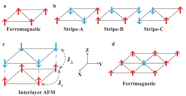
Supplementary Figure 2: a-d show the sketches of different magnetic configurations. The energies of a ferromagnetic and b stripe states are also calculated in enlarged supercells in order to compare with other states in c and d directly (see Supplementary Table 2).

Supplementary Tabel 2: Magnetic space group (MSG) numbers and energies of different configurations, calculated by DFT+U method.

Magnetic Configuration	MSG Number	Supercell Size	Energy/eV	Difference/eV
Ferromagnetic	164.89	$1\times 1\times 2$	-184.90846	—–
Interlayer-AFM	165.96	$1\times 1\times 2$	-184.90828	0.00018
Ferromagnetic	164.89	$2\times 2\times 1$	-368.29838	0.00000
Ferrimagnetic	164.89	$2\times 2\times 1$	-368.59576	-0.29738
AFM stripe-A	14.83	$2\times 2\times 1$	-368.30225	-0.00387
AFM stripe-B	14.83	$2\times 2\times 1$	-368.30227	-0.00389
AFM stripe-C	14.83	$2\times 2\times 1$	-368.30226	-0.00388

In Supplementary Figure 3 we adopt an alternative way to estimate the spin exchange couplings [71, 17]. In Supplementary Figure 3a the orbital projected band structure of Na₂BaCo(PO₄)₂ with Hubbard $U_{\rm eff}=2$ eV is shown. We see near the Fermi energy are mainly 3$d$ electron bands, well separated from the other bands. We choose the 3$d$ orbitals as the bases of Wannier functions to compute the major hopping amplitudes between the near neighboring Wannier centers, and the exchange coupling $J_{1}$ between a pair of Co²⁺ ions can be estimated as $J_{1}=(16/81)t^{2}/U$ [17]. The resulting $J_{1}$ with $U_{\rm eff}$ values below 2.5 eV are plotted in Supplementary Figure 3b, from which we find that $J_{1}$ decreases rapidly as $U_{\rm eff}$ increases. For $U_{\rm eff}$ above 2.5 eV, the Co 3$d$-orbitals are mixed with the oxygen 2$p$-orbitals, and the simple formula for $J_{1}$ estimation becomes no longer applicable. Therefore we perform a (second-order) polynomial fit of the DFT results up to $2.5$ eV, and extrapolate to large $U_{\rm eff}$. We find $J_{1}$ becomes about 2.4 K for $U_{\rm eff}=5$ eV, in agreement with the energy scales of determined spin exchange in the main text.

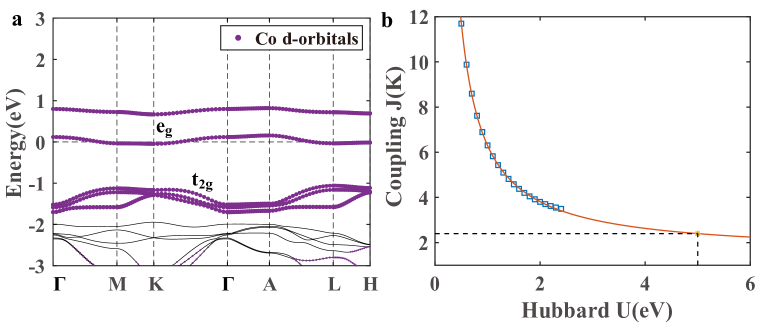
Supplementary Figure 3: a The Co 3$d$-orbital projected band structure of Na₂BaCo(PO₄)₂. b The estimated exchange strengths $J_{1}$ drawn from the Wannier functions are plotted vs. the Hubbard $U$. The blue dots are the Wannier functions results, and the red line represent the second-order polynomial extrapolation.

Nevertheless, note the true exchange path is a super-super exchange through the Co-O-O-Co path shown below instead of the direct Co-Co exchange. In Supplementary Figure 4 we provide the charge density contour obtained by DFT+U calculations, which visualize the spin exchange path. The minimum charge density in the Co-O-O-Co path in Supplementary Figure 4a is about $0.03~{}{\rm e}~{}{\rm Bohr}^{-3}$. The out-of-plane contour map in Supplementary Figure 4b shows the very weak overlap of charge density distributions between two adjacent triangular planes, and the minimum charge density is about $0.004~{}{\rm e}~{}{\rm Bohr}^{-3}$ in the supposed super-super-super exchange path indicated by the dash line.

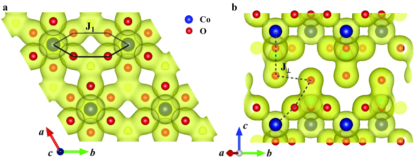
Supplementary Figure 4: The intra- and inter-plane charge density contour maps. The red and blue dots represent respectively the O and Co ions. The solid lines in a denote the super-super exchange path between a pair of near neighbor Co ions within the same triangular plane. The dashed lines in b denote the possible super-super-super exchange path of two Co ions in adjacent planes.

Supplementary Note 3 Crystal symmetry analysis and the effective spin Hamiltonian

In this section, we use the symmetries of the material to constrain the possible exchange interactions between two neighbor Co²⁺ ions.

• The Co²⁺ ions occupy the Wychoff position $1b$ of the space group $P\bar{3}m1$. Its site symmetry group is $\bar{3}m$ (see, Supplementary Figure 1a of the main text), which is generated by a 3-fold rotation w.r.t. the crystallographic ${c}$ axis, a two-fold rotation w.r.t. the nearest neighbor (NN) bond, and the inversion.

• The center of two neighboring Co²⁺ ions in the same basal planes corresponds to the Wyckoff position $3f$ with site symmetry group $2/m$. The site symmetry group is generated by a two-fold rotation w.r.t. the NN bond and the inversion.

We consider the exchange interactions between magnetic ions in the same basal plane. There are three translation-inequivalent NN bonds, which are related by the three-fold rotations. Therefore it is sufficient to determine the exchange interaction on one bond and obtain the interactions on the other two by rotations.

Let $i$, $j$ denote two NN sites of Co²⁺. Let $\hat{n}_{ij}$ be the unit vector that points form site $i$ to site $j$ and $\hat{\epsilon}_{ij}\equiv{c}\times\hat{n}_{ij}$. The most general bilinear exchange interaction between these two sites reads: $H_{ij}=\sum_{\alpha\beta}J^{\alpha\beta}S_{i}^{\alpha}S_{j}^{\beta}$, where $\alpha,~{}\beta$ run over $\{\hat{n}_{ij},\hat{\epsilon}_{ij},{c}\}$. Now consider all the symmetries that preserve the bond $ij$. The inversion symmetry w.r.t. the center of the bond implies that $J^{\alpha\beta}=J^{\beta\alpha}$. Furthermore, the 2-fold rotation w.r.t. the bond itself implies $J_{n\epsilon}=J_{nc}=0$. We are left with four independent, symmetry-allowed interactions $H_{ij}=J_{H}\textbf{S}_{i}\cdot\textbf{S}_{j}+J_{I}({c}\cdot\textbf{S}_{i})({c}\cdot\textbf{S}_{j})+J_{nn}(\hat{n}_{ij}\cdot\textbf{S}_{i})(\hat{n}_{ij}\cdot\textbf{S}_{j})+J_{\epsilon c}[({c}\cdot\textbf{S}_{i})(\hat{\epsilon}_{ij}\cdot\textbf{S}_{j})+({c}\cdot\textbf{S}_{j})(\hat{\epsilon}_{ij}\cdot\textbf{S}_{i})]$. We recognize the first term as the Heisenberg exchange, the second Ising, the third pseudo-dipolar, and the last “symmetric off-diagonal” exchange interaction.

To align with the convention in previous works [24, 25, 26], we recast the Hamiltonian via the following transformation: $J_{xy}=J_{H}+\frac{1}{2}J_{nn}$, $J_{z}=J_{H}+J_{I}$, $J_{\rm PD}=\frac{1}{4}J_{nn}$, $J_{\Gamma}=J_{n\epsilon}$. We note, through such transformation, the parameters become $J_{\pm\pm}\equiv J_{\rm PD}$ and $J_{z\pm}\equiv J_{\Gamma}$ as adopted in Refs. [24, 25, 26]. Here we define $S^{x}$ and $S^{z}$, i.e., respectively spin (1,0,0) and (0,0,1) directions, as along the $a-$ and $c-$ axes, and arrive at the Hamiltonian in Eq. (1) of the main text.

Another way to set up the coordinate system is taking the spin $(1,1,1)$ direction parallel to $c$-axis, and spin $(-1,-1,2)$ direction parallel to $a$-axis. Thus the 3-fold rotation operation is a cyclic permutation of three components of the spin operator. For $\hat{n}_{ij}=\frac{1}{\sqrt{6}}(-1,-1,2)$, i.e., along the $a$-axis, one has

$$\begin{split}H_{ij}=&J_{H}\textbf{S}_{i}\cdot\textbf{S}_{j}+\frac{J_{I}}{3}(S_{i}^{x}+S_{i}^{y}+S_{i}^{z})(S_{j}^{x}+S_{j}^{y}+S_{j}^{z})+\frac{J_{nn}}{6}(-S_{i}^{x}-S_{i}^{y}+2S_{i}^{z})(-S_{j}^{x}-S_{j}^{y}+2S_{j}^{z})\\ &+\frac{J_{\epsilon c}}{6}\{(S_{i}^{x}+S_{i}^{y}+S_{i}^{z})(S_{j}^{x}-S_{j}^{y})+(S_{i}^{x}-S_{i}^{y})(S_{j}^{x}+S_{j}^{y}+S_{j}^{z})\}.\end{split}$$ (2)

The $J_{nn}$ and $J_{\epsilon c}$ terms can lead to a bond-dependent, Kitaev-type, interaction in the system, which, however, are found to be negligible in our spin model established in the main text.

Supplementary Note 4 XTRG results of TLAF model under nonzero fields

Besides the zero-field magnetic specific heat $C_{\rm m}$ presented in the main text, here we present comparisons between the simulated $C_{\rm m}$ under various magnetic fields along the $c$ axis with the experimental results. As shown in Supplementary Figure 5, the model calculations and experiments are in very good agreement whenever the two experimental curves [14, 15] coincide. In the lower temperature range, our simulated data can well reproduce the peak positions in quantitative agreement with experiment (c.f., Supplementary Figure 5a, b).

In practical calculations, we perform XTRG calculations on two different lattice geometries (c.f. Fig 6), i.e., YC$4\times 6$ (used mainly in the automatic parameter searching) and YC$6\times 9$ (larger-size calculations for validation). As shown in Fig 5a, above $T_{\text{cut}}=1$ K, no significant difference between the two simulated data with Lattice 1 and 2 can be observed.

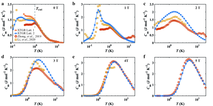
Supplementary Figure 5: a-f The magnetic specific heat of XTRG simulations under various fields along the $c$ axis, and comparisons to the experimental data (Zhong, et al., 2019 [14], and Li, et al., 2020 [15]). The simulations are performed on YC$4\times 6$ (Lattice 1) and YC$6\times 9$ (Lattice 2, see Supplementary Figure 6).

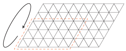
Supplementary Figure 6: The YC$6\times 9$ and YC$4\times 6$ (within the orange dash line) lattice geometries that are used in XTRG simulations. The arrow indicates the periodic boundary condition along the circumference of the cylinder.

Supplementary Note 5 Semi-Classical analysis of the TLH model under out-of-plane fields

It is known that the classical ground state of the TLAF model shows a three-sub-lattice structure. In the presence of a magnetic field, the model shows a sequence of phase transitions. Nevertheless, the said three-sub-lattice structure is preserved.

Suppose the interactions $J_{xy}$ and $J_{z}$ are dominant. It is then natural to assume the subdominant interactions $J_{\rm PD}$ and $J_{\Gamma}$ do not change the three-sub-lattice structure — in other words, the magnetic unit cell remains to be $\sqrt{3}\times\sqrt{3}$. We now show that the classical magnetic phase diagram will be independent of $J_{\rm PD}$ and $J_{\Gamma}$.

Let $\bf{S}_{A,B,C}$ donate the classical spin vector in the sub-lattices A, B, and C, respectively. The classical energy reads:

$$\begin{split}H=&\frac{N}{3}(J_{a}^{\alpha\beta}+J_{b}^{\alpha\beta}+J_{c}^{\alpha\beta})S_{A}^{\alpha}S_{B}^{\beta}+(B,C)+(C,A)-\frac{N\mu_{0}}{3}g_{\alpha\beta}B^{\alpha}(S_{A}^{\beta}+S_{B}^{\beta}+S_{C}^{\beta})\\ =&N(J_{xy}S_{A}^{x}S_{B}^{x}+J_{xy}S_{A}^{y}S_{B}^{y}+J_{z}S_{A}^{z}S_{B}^{z})+(B,C)+(C,A)-\frac{N\mu_{0}}{3}g_{\alpha\beta}B^{\alpha}(S_{A}^{\beta}+S_{B}^{\beta}+S_{C}^{\beta}),\end{split}$$ (3)

where $N$ is the number of lattice sites, $g_{\alpha\beta}$ is the general Landé factor, and $B^{\alpha}$ is the magnetic field along $\alpha$ direction. We see that the contributions form $J_{\rm PD}$ and $J_{\Gamma}$ cancel. An immediate consequence is that the classical ground states show an accidental U(1) symmetry w.r.t. the $z$ axis, which will be lifted by quantum fluctuations through the order by disorder mechanism.

We now review the classical magnetic ground states of the TLAF model with easy-axis anisotropy, i.e., $J_{z}>J_{xy}>0$. As the out-of-plane field $B\parallel c$ increases, the model shows a sequence of four magnetic phases: the Y state, the up-up-down state, the V state, and the fully polarized state. These phase are separated by three critical fields, which we label $B_{c1}$, $B_{c2}$, and $B_{c3}$,

We would like to determine the values of these critical fields. Beginning with $B_{c3}$, let us consider the stability of the polarized phase. We write:

$$S_{A}^{x}=\sqrt{S}x_{A},~{}~{}~{}S_{A}^{y}=\sqrt{S}y_{A},~{}~{}~{}S_{A}^{z}=S-\frac{x_{A}^{2}+y_{A}^{2}}{2}.$$ (4)

The other two spins are written in the same manner. Substituting Eq. (4) above into the expression of energy [Eq. (3)] and expand to the quadratic order:

$$H=\frac{N}{2}(x^{\text{T}}M_{x}x+y^{\text{T}}M_{y}y),$$ (5)

where $x=(x_{A},x_{B},x_{C})^{\text{T}}$ and $y=(y_{A},y_{B},y_{C})^{\text{T}}$ . The Hessian matrix:

$$M_{x}=M_{y}=\left(\begin{matrix}\frac{g_{z}\mu_{0}B}{3}-2J_{z}S&J_{xy}S&J_{xy}S\\ J_{xy}S&\frac{g_{z}\mu_{0}B}{3}-2J_{z}S&J_{xy}S\\ J_{xy}S&J_{xy}S&\frac{g_{z}\mu_{0}B}{3}-2J_{z}S\end{matrix}\right)$$ (6)

The three eigenvalues are:

$$\lambda_{1,2}=\frac{g_{z}\mu_{0}B}{3}-2J_{z}S-J_{xy}S,~{}~{}~{}\lambda_{3}=\frac{g_{z}\mu_{0}B}{3}-2J_{z}S+2J_{xy}S.$$ (7)

The stability of polarized state requires $\lambda_{1,2}\geq 0$, which implies:

$$g_{z}\mu_{0}B_{c3}=3(J_{xy}+2J_{z})S.$$ (8)

We then determine $B_{c1}$ and $B_{c2}$. To this end, consider the stability of the UUD phase. We write:

$$\begin{split}S_{A}^{x}=\sqrt{S}x_{A},~{}~{}~{}S_{A}^{y}&=-\sqrt{S}y_{A},~{}~{}~{}S_{A}^{z}=-S+\frac{x_{A}^{2}+y_{A}^{2}}{2};\\ S_{B,C}^{x}=\sqrt{S}x_{B,C},~{}~{}~{}S_{B,C}^{y}&=\sqrt{S}y_{B,C},~{}~{}~{}S_{B,C}^{z}=S-\frac{x_{B,C}^{2}+y_{B,C}^{2}}{2}.\end{split}$$ (9)

The energy is given by:

$$H=\frac{N}{2}(x^{\text{T}}M_{x}x+y^{\text{T}}M_{y}y),$$ (10)

where the Hessian matrices:

$$M_{x}=\left(\begin{matrix}2J_{z}S-\frac{g_{z}\mu_{0}B}{3}&J_{xy}S&J_{xy}S\\ J_{xy}S&\frac{g_{z}\mu_{0}B}{3}&J_{xy}S\\ J_{xy}S&J_{xy}S&\frac{g_{z}\mu_{0}B}{3}\end{matrix}\right),M_{y}=\left(\begin{matrix}2J_{z}S-\frac{g_{z}\mu_{0}B}{3}&-J_{xy}S&-J_{xy}S\\ -J_{xy}S&\frac{g_{z}\mu_{0}B}{3}&J_{xy}S\\ -J_{xy}S&J_{xy}S&\frac{g_{z}\mu_{0}B}{3}\end{matrix}\right).$$ (11)

The eigenvalues of $M_{x}$ and $M_{y}$ are identical. They are given by:

$$\lambda_{1}=\frac{g_{z}\mu_{0}B}{3}-J_{xy},~{}~{}~{}\lambda_{2,3}=J_{z}S+\frac{J_{xy}S}{2}\pm\sqrt{(J_{z}S-\frac{g_{z}\mu_{0}B}{3}-\frac{J_{xy}S}{2})^{2}+2(J_{xy}S)^{2}}.$$ (12)

The stability condition requires:

$$\frac{g_{z}\mu_{0}B}{3}-J_{xy}\geq 0,~{}~{}~{}(J_{z}S+\frac{J_{xy}S}{2})^{2}\geq(J_{z}S-\frac{g_{z}\mu_{0}B}{3}-\frac{J_{xy}S}{2})^{2}+2(J_{xy}S)^{2}$$ (13)

We deduce:

$$g_{z}\mu_{0}B_{c1}=3J_{xy}S,$$ (14)

$$g_{z}\mu_{0}B_{c2}=3(J_{z}-\frac{J_{xy}}{2}+\sqrt{J_{z}^{2}+J_{z}J_{xy}-\frac{7}{4}J_{xy}^{2}})S.$$ (15)

References

- Anderson [1973] P. W. Anderson, Resonating valence bonds: A new kind of insulator?, Mater. Res. Bull. 8, 153 (1973).
- Chubukov and Golosov [1991] A. V. Chubukov and D. I. Golosov, Quantum theory of an antiferromagnet on a triangular lattice in a magnetic field, J. Phys.: Condens. Matter 3, 69 (1991).
- Collins and Petrenko [1997] M. F. Collins and O. A. Petrenko, Review/synthèse: Triangular antiferromagnets, Can. J. Phys. 75, 605 (1997).
- Starykh [2015] O. A. Starykh, Unusual ordered phases of highly frustrated magnets: a review, Rep. Prog. Phys. 78, 052502 (2015).
- Wessel and Troyer [2005] S. Wessel and M. Troyer, Supersolid hard-core Bosons on the triangular lattice, Phys. Rev. Lett. 95, 127205 (2005).
- Melko et al. [2005] R. G. Melko, A. Paramekanti, A. A. Burkov, A. Vishwanath, D. N. Sheng, and L. Balents, Supersolid order from disorder: Hard-core Bosons on the triangular lattice, Phys. Rev. Lett. 95, 127207 (2005).
- Heidarian and Damle [2005] D. Heidarian and K. Damle, Persistent supersolid phase of hard-core Bosons on the triangular lattice, Phys. Rev. Lett. 95, 127206 (2005).
- Boninsegni and Prokof’ev [2005] M. Boninsegni and N. Prokof’ev, Supersolid phase of hard-core Bosons on a triangular lattice, Phys. Rev. Lett. 95, 237204 (2005).
- Heidarian and Paramekanti [2010] D. Heidarian and A. Paramekanti, Supersolidity in the triangular lattice spin- XXZ model: A variational perspective, Phys. Rev. Lett. 104, 015301 (2010).
- Wang et al. [2009] F. Wang, F. Pollmann, and A. Vishwanath, Extended supersolid phase of frustrated hard-core Bosons on a triangular lattice, Phys. Rev. Lett. 102, 017203 (2009).
- Jiang et al. [2009] H. C. Jiang, M. Q. Weng, Z. Y. Weng, D. N. Sheng, and L. Balents, Supersolid order of frustrated hard-core Bosons in a triangular lattice system, Phys. Rev. B 79, 020409 (2009).
- Yamamoto et al. [2014] D. Yamamoto, G. Marmorini, and I. Danshita, Quantum phase diagram of the triangular-lattice XXZ model in a magnetic field, Phys. Rev. Lett. 112, 127203 (2014).
- Yamamoto et al. [2019] D. Yamamoto, G. Marmorini, M. Tabata, K. Sakakura, and I. Danshita, Magnetism driven by the interplay of fluctuations and frustration in the easy-axis triangular XXZ model with transverse fields, Phys. Rev. B 100, 140410 (2019).
- Zhong et al. [2019] R. Zhong, S. Guo, G. Xu, Z. Xu, and R. J. Cava, Strong quantum fluctuations in a quantum spin liquid candidate with a Co-based triangular lattice, Proc. Natl Acad. Sci. USA 116, 14505 (2019).
- Li et al. [2020a] N. Li, Q. Huang, X. Y. Yue, W. J. Chu, Q. Chen, E. S. Choi, X. Zhao, H. D. Zhou, and X. F. Sun, Possible itinerant excitations and quantum spin state transitions in the effective spin-1/2 triangular-lattice antiferromagnet Na2BaCo(PO4)2, Nat. Commun. 11, 4216 (2020a).
- Lee et al. [2021] S. Lee, C. H. Lee, A. Berlie, A. D. Hillier, D. T. Adroja, R. Zhong, R. J. Cava, Z. H. Jang, and K.-Y. Choi, Temporal and field evolution of spin excitations in the disorder-free triangular antiferromagnet 2, Phys. Rev. B 103, 024413 (2021).
- Wellm et al. [2021] C. Wellm, W. Roscher, J. Zeisner, A. Alfonsov, R. Zhong, R. J. Cava, A. Savoyant, R. Hayn, J. van den Brink, B. Büchner, O. Janson, and V. Kataev, Frustration enhanced by Kitaev exchange in a triangular antiferromagnet, Phys. Rev. B 104, L100420 (2021).
- Liu and Khaliullin [2018a] H. Liu and G. Khaliullin, Pseudospin exchange interactions in cobalt compounds: Possible realization of the Kitaev model, Phys. Rev. B 97, 014407 (2018a).
- Yu et al. [2021a] S. Yu, Y. Gao, B.-B. Chen, and W. Li, Learning the effective spin Hamiltonian of a quantum magnet, Chin. Phys. Lett. 38, 097502 (2021a).
- Chen et al. [2019a] L. Chen, D.-W. Qu, H. Li, B.-B. Chen, S.-S. Gong, J. von Delft, A. Weichselbaum, and W. Li, Two temperature scales in the triangular lattice Heisenberg antiferromagnet, Phys. Rev. B 99, 140404(R) (2019a).
- Li et al. [2019] H. Li, B.-B. Chen, Z. Chen, J. von Delft, A. Weichselbaum, and W. Li, Thermal tensor renormalization group simulations of square-lattice quantum spin models, Phys. Rev. B 100, 045110 (2019).
- White [1992] S. R. White, Density matrix formulation for quantum renormalization groups, Phys. Rev. Lett. 69, 2863 (1992).
- Tinkham [2003] M. Tinkham, Group theory and quantum mechanic (Mineola, N.Y.: Dover Publications, 2003).
- Li et al. [2015] Y. Li, G. Chen, W. Tong, L. Pi, J. Liu, Z. Yang, X. Wang, and Q. Zhang, Rare-earth triangular lattice spin liquid: A single-crystal study of , Phys. Rev. Lett. 115, 167203 (2015).
- Li et al. [2016] Y.-D. Li, X. Wang, and G. Chen, Anisotropic spin model of strong spin-orbit-coupled triangular antiferromagnets, Phys. Rev. B 94, 035107 (2016).
- Zhu et al. [2018] Z. Zhu, P. A. Maksimov, S. R. White, and A. L. Chernyshev, Topography of spin liquids on a triangular lattice, Phys. Rev. Lett. 120, 207203 (2018).
- Chen et al. [2018] B.-B. Chen, L. Chen, Z. Chen, W. Li, and A. Weichselbaum, Exponential thermal tensor network approach for quantum lattice models, Phys. Rev. X 8, 031082 (2018).
- Yamamoto et al. [2015] D. Yamamoto, G. Marmorini, and I. Danshita, Microscopic model calculations for the magnetization process of layered triangular-lattice quantum antiferromagnets, Phys. Rev. Lett. 114, 027201 (2015).
- Sellmann et al. [2015] D. Sellmann, X.-F. Zhang, and S. Eggert, Phase diagram of the antiferromagnetic XXZ model on the triangular lattice, Phys. Rev. B 91, 081104 (2015).
- Stephan and Southern [2000] W. Stephan and B. W. Southern, Monte Carlo study of the anisotropic Heisenberg antiferromagnet on the triangular lattice, Phys. Rev. B 61, 11514 (2000).
- Miyashita and Kawamura [1985] S. Miyashita and H. Kawamura, Phase transitions of anisotropic Heisenberg antiferromagnets on the triangular lattice, J. Phys. Soc. Jpn. 54, 3385 (1985).
- Sheng and Henley [1992] Q. Sheng and C. L. Henley, Ordering due to disorder in a triangular Heisenberg antiferromagnet with exchange anisotropy, J. Phys.: Condens. Matter 4, 2937 (1992).
- Seabra and Shannon [2011] L. Seabra and N. Shannon, Competition between supersolid phases and magnetization plateaus in the frustrated easy-axis antiferromagnet on a triangular lattice, Phys. Rev. B 83, 134412 (2011).
- Kim and Chan [2004] E. Kim and M. H. W. Chan, Probable observation of a supersolid helium phase, Nature 427, 225 (2004).
- Kim and Chan [2012] D. Y. Kim and M. H. W. Chan, Absence of supersolidity in solid helium in porous vycor glass, Phys. Rev. Lett. 109, 155301 (2012).
- Li et al. [2017] J.-R. Li, J. Lee, W. Huang, S. Burchesky, B. Shteynas, F. Ç. Top, A. O. Jamison, and W. Ketterle, A stripe phase with supersolid properties in spin–orbit-coupled bose–einstein condensates, Nature 543, 91 (2017).
- Léonard et al. [2017] J. Léonard, A. Morales, P. Zupancic, T. Donner, and T. Esslinger, Monitoring and manipulating higgs and goldstone modes in a supersolid quantum gas, Science 358, 1415 (2017).
- Tanzi et al. [2019] L. Tanzi, S. M. Roccuzzo, E. Lucioni, F. Famà, A. Fioretti, C. Gabbanini, G. Modugno, A. Recati, and S. Stringari, Supersolid symmetry breaking from compressional oscillations in a dipolar quantum gas, Nature 574, 382 (2019).
- Norcia et al. [2021] M. A. Norcia, C. Politi, L. Klaus, E. Poli, M. Sohmen, M. J. Mark, R. N. Bisset, L. Santos, and F. Ferlaino, Two-dimensional supersolidity in a dipolar quantum gas, Nature 596, 357 (2021).
- Doi et al. [2004] Y. Doi, Y. Hinatsu, and K. Ohoyama, Structural and magnetic properties of pseudo-two-dimensional triangular antiferromagnets Ba3MSb2O9 (M = Mn, Co, and Ni), J. Phys.: Condens. Matter 16, 8923 (2004).
- Shirata et al. [2012] Y. Shirata, H. Tanaka, A. Matsuo, and K. Kindo, Experimental realization of a spin- triangular-lattice Heisenberg antiferromagnet, Phys. Rev. Lett. 108, 057205 (2012).
- Zhou et al. [2012] H. D. Zhou, C. Xu, A. M. Hallas, H. J. Silverstein, C. R. Wiebe, I. Umegaki, J. Q. Yan, T. P. Murphy, J.-H. Park, Y. Qiu, J. R. D. Copley, J. S. Gardner, and Y. Takano, Successive phase transitions and extended spin-excitation continuum in the triangular-lattice antiferromagnet Ba3CoSb2O9, Phys. Rev. Lett. 109, 267206 (2012).
- Susuki et al. [2013] T. Susuki, N. Kurita, T. Tanaka, H. Nojiri, A. Matsuo, K. Kindo, and H. Tanaka, Magnetization process and collective excitations in the triangular-lattice Heisenberg antiferromagnet Ba3CoSb2O9, Phys. Rev. Lett. 110, 267201 (2013).
- Ma et al. [2016] J. Ma, Y. Kamiya, T. Hong, H. B. Cao, G. Ehlers, W. Tian, C. D. Batista, Z. L. Dun, H. D. Zhou, and M. Matsuda, Static and dynamical properties of the spin- equilateral triangular-lattice antiferromagnet Ba3CoSb2O9, Phys. Rev. Lett. 116, 087201 (2016).
- Sera et al. [2016] A. Sera, Y. Kousaka, J. Akimitsu, M. Sera, T. Kawamata, Y. Koike, and K. Inoue, triangular-lattice antiferromagnets O9 and : Role of spin-orbit coupling, crystalline electric field effect, and Dzyaloshinskii-Moriya interaction, Phys. Rev. B 94, 214408 (2016).
- Ito et al. [2017] S. Ito, N. Kurita, H. Tanaka, S. Ohira-Kawamura, K. Nakajima, S. Itoh, K. Kuwahara, and K. Kakurai, Structure of the magnetic excitations in the spin-1/2 triangular-lattice Heisenberg antiferromagnet Ba3CoSb2O9, Nat. Commun. 8, 235 (2017).
- Kamiya et al. [2018] Y. Kamiya, L. Ge, T. Hong, Y. Qiu, D. L. Quintero-Castro, Z. Lu, H. B. Cao, M. Matsuda, E. S. Choi, C. D. Batista, M. Mourigal, H. D. Zhou, and J. Ma, The nature of spin excitations in the one-third magnetization plateau phase of , Nat. Commun. 9, 2666 (2018).
- Rawl et al. [2017] R. Rawl, L. Ge, H. Agrawal, Y. Kamiya, C. R. Dela Cruz, N. P. Butch, X. F. Sun, M. Lee, E. S. Choi, J. Oitmaa, C. D. Batista, M. Mourigal, H. D. Zhou, and J. Ma, : A spin- triangular-lattice Heisenberg antiferromagnet in the two-dimensional limit, Phys. Rev. B 95, 060412(R) (2017).
- Cui et al. [2018] Y. Cui, J. Dai, P. Zhou, P. S. Wang, T. R. Li, W. H. Song, J. C. Wang, L. Ma, Z. Zhang, S. Y. Li, G. M. Luke, B. Normand, T. Xiang, and W. Yu, Mermin-Wagner physics, phase diagram, and candidate quantum spin-liquid phase in the spin- triangular-lattice antiferromagnet , Phys. Rev. Materials 2, 044403 (2018).
- Chen et al. [2019b] L. Chen, D.-W. Qu, H. Li, B.-B. Chen, S.-S. Gong, J. von Delft, A. Weichselbaum, and W. Li, Two-temperature scales in the triangular-lattice Heisenberg antiferromagnet, Phys. Rev. B 99, 140404 (2019b).
- Hu et al. [2020] Z. Hu, Z. Ma, Y.-D. Liao, H. Li, C. Ma, Y. Cui, Y. Shangguan, Z. Huang, Y. Qi, W. Li, Z. Y. Meng, J. Wen, and W. Yu, Evidence of the Berezinskii-Kosterlitz-Thouless phase in a frustrated magnet, Nat. Commun. 11, 5631 (2020).
- Modic et al. [2021] K. A. Modic, R. D. McDonald, J. P. C. Ruff, M. D. Bachmann, Y. Lai, J. C. Palmstrom, D. Graf, M. K. Chan, F. F. Balakirev, J. B. Betts, G. S. Boebinger, M. Schmidt, M. J. Lawler, D. A. Sokolov, P. J. W. Moll, B. J. Ramshaw, and A. Shekhter, Scale-invariant magnetic anisotropy in RuCl3 at high magnetic fields, Nat. Phys. 17, 240 (2021).
- Rost et al. [2009] A. W. Rost, R. S. Perry, J.-F. Mercure, A. P. Mackenzie, and S. A. Grigera, Entropy landscape of phase formation associated with quantum criticality in Sr3Ru2O7, Science 325, 1360 (2009).
- Fortune et al. [2009] N. A. Fortune, S. T. Hannahs, Y. Yoshida, T. E. Sherline, T. Ono, H. Tanaka, and Y. Takano, Cascade of magnetic-field-induced quantum phase transitions in a spin- triangular-lattice antiferromagnet, Phys. Rev. Lett. 102, 257201 (2009).
- Bachus et al. [2020] S. Bachus, D. A. S. Kaib, Y. Tokiwa, A. Jesche, V. Tsurkan, A. Loidl, S. M. Winter, A. A. Tsirlin, R. Valentí, and P. Gegenwart, Thermodynamic perspective on field-induced behavior of -RuCl3, Phys. Rev. Lett. 125, 097203 (2020).
- Chen et al. [2017] B.-B. Chen, Y.-J. Liu, Z. Chen, and W. Li, Series-expansion thermal tensor network approach for quantum lattice models, Phys. Rev. B 95, 161104(R) (2017).
- Li et al. [2020b] H. Li, Y.-D. Liao, B.-B. Chen, X.-T. Zeng, X.-L. Sheng, Y. Qi, Z. Y. Meng, and W. Li, Kosterlitz-Thouless melting of magnetic order in the triangular quantum Ising material TmMgGaO4, Nat. Commun. 11, 1111 (2020b).
- Li et al. [2020c] H. Li, D.-W. Qu, H.-K. Zhang, Y.-Z. Jia, S.-S. Gong, Y. Qi, and W. Li, Universal thermodynamics in the Kitaev fractional liquid, Phys. Rev. Research 2, 043015 (2020c).
- Li et al. [2021] H. Li, H.-K. Zhang, J. Wang, H.-Q. Wu, Y. Gao, D.-W. Qu, Z.-X. Liu, S.-S. Gong, and W. Li, Identification of magnetic interactions and high-field quantum spin liquid in -RuCl3, Nat. Commun. 12, 4007 (2021).
- Chen et al. [2021] B.-B. Chen, C. Chen, Z. Chen, J. Cui, Y. Zhai, A. Weichselbaum, J. von Delft, Z. Y. Meng, and W. Li, Quantum many-body simulations of the two-dimensional Fermi-Hubbard model in ultracold optical lattices, Phys. Rev. B 103, L041107 (2021).
- Lin et al. [2022] X. Lin, B.-B. Chen, W. Li, Z. Y. Meng, and T. Shi, Exciton proliferation and fate of the topological mott insulator in a twisted bilayer graphene lattice model, Phys. Rev. Lett. 128, 157201 (2022).
- Yu et al. [2021b] S. Yu, Y. Gao, B.-B. Chen, and W. Li, QMagen (2021b), https://github.com/QMagen.
- Abragam and Bleaney [1970] A. Abragam and B. Bleaney, Electron paramagnetic resonance of transition ions (Oxford: Clarendon P, 1970).
- Scheie [2021] A. Scheie, PyCrystalField: software for calculation, analysis and fitting of crystal electric field Hamiltonians, J. Appl. Cryst. 54, 356 (2021).
- Koseki et al. [2019] S. Koseki, N. Matsunaga, T. Asada, M. W. Schmidt, and M. S. Gordon, Spin–orbit coupling constants in atoms and ions of transition elements: Comparison of effective core potentials, model core potentials, and all-electron methods, J. Phys. Chem. A 123, 2325 (2019).
- ato [2020] National institute of standards and technology, atomic spectra data base (2020).
- Anisimov et al. [1991] V. I. Anisimov, J. Zaanen, and O. K. Andersen, Band theory and mott insulators: Hubbard U instead of stoner I, Phys. Rev. B 44, 943 (1991).
- Anisimov et al. [1993] V. I. Anisimov, I. V. Solovyev, M. A. Korotin, M. T. Czyżyk, and G. A. Sawatzky, Density-functional theory and NiO photoemission spectra, Phys. Rev. B 48, 16929 (1993).
- Dudarev et al. [1998] S. L. Dudarev, G. A. Botton, S. Y. Savrasov, C. J. Humphreys, and A. P. Sutton, Electron-energy-loss spectra and the structural stability of nickel oxide: An LSDA+U study, Phys. Rev. B 57, 1505 (1998).
- Perdew et al. [1996] J. P. Perdew, K. Burke, and M. Ernzerhof, Generalized gradient approximation made simple, Phys. Rev. Lett. 77, 3865 (1996).
- Liu and Khaliullin [2018b] H. Liu and G. Khaliullin, Pseudospin exchange interactions in cobalt compounds: Possible realization of the kitaev model, Phys. Rev. B 97, 014407 (2018b).