Precision study of the continuum SU(3) Yang-Mills theory: how to use parallel tempering to improve on supercritical slowing down for first order phase transitions

Abstract

We perform large scale simulations to characterize the transition in quenched QCD. It is shown by a rigorous finite size scaling that the transition is of first order. After this qualitative feature quantitative results are obtained with unprecedented precision: we calculate the transition temperature $w_{0}T_{c}$=0.25384(23) – which is the first per-mill accurate result in QCD thermodynamics – and the latent heat $\Delta E/T_{c}^{4}$=1.025(21)(27), in both cases carrying out controlled continuum and infinite volume extrapolations. As it is well known the cost of lattice simulations explodes in the vicinity of phase transitions, a phenomenon called critical slowing down for second order phase transitions and supercritical slowing down for first order phase transitions. We show that a generalization of the parallel tempering algorithm of Marinari and Parisi [Europhys. Lett. 19, 451 (1992)] originally for spin systems can efficiently overcome these difficulties even if the transition is of first order, like in the case of QCD without quarks, or with very heavy quarks. We also report on our investigations on the autocorrelation times and other details.

I Introduction

There is no doubt in the theoretical physics community that the SU(3) Yang-Mills theory, or QCD without quarks, features a first order phase transition. The transition takes place at a temperature around 290 MeV, the precise value strongly depending on the choice of the variable to set the scale. It separates the cold confining phase from a hot phase with spontaneously broken center symmetry.

In the context of full QCD this transition was expected to happen as a consequence of Hagedorn’s exponential spectrum [1], and a first phase diagram was drawn in Ref. [2]. Later, the necessity of a transition was derived from the underlying quantum field theory and linked to the center of the gauge group [3]. In contrast to the well known crossover transition in full QCD [4], the order of the transition between the confining and weak-coupling phases was argued to be first order in the quarkless SU(3) theory [5, 6]. The main argument relies on the $Z(3)$ symmetry of the three-dimensional effective theory, and that no stable renormalization group fixed point is known with that symmetry. Such an effective theory has already been studied extensively in the context of the Potts model [7].

Our main motivation to study the transition of the SU(3) Yang-Mills theory is the exploration of the so-called “Columbia plot”, a diagram showing the nature of the QCD transition as a function of the light and strange quark masses $m_{u}=m_{d}=m_{l},m_{s}$. Because of the absence of an exact $Z(3)$ symmetry for finite quark mass the transition will turn into crossover below a certain critical mass [6]. This mass was estimated using Dyson-Schwinger equations [8] and in effective models [9]. In the opposing corner of the Columbia plot, referred to as the “chiral limit”, one again expects a first order transition for three or more massless flavors, following from the $\epsilon$ expansion of a linear $\sigma$ model [10]. This diagram was first studied in lattice QCD by the Columbia group [11] and has been a subject of intense research ever since. In terms of simulation costs the study of the upper right corner is considerably simpler than working close to the chiral limit, partly because of the slow convergence of the iterative solvers, partly because of the more elaborate fermion formulations that the chiral limit requires. However, simulations are in progress even near the chiral corner, and recent results challenge the theoretical assumptions on the phase diagram [12].

But even the upper right corner is non-trivial to simulate. It has been addressed using reweighting from quenched QCD [13, 14], reweighting from a leading order hopping-term expansion [15] or a three-dimensional effective theory for the Polyakov loop [16], or with direct simulations [17, 18]. While these results are promising and appear to be consistent with matrix models [9], a continuum extrapolation could not be achieved, yet.

The main difficulty in pinpointing the critical mass is not simply coming from the presence of quarks, as the iterative solvers converge very quickly in these studies. The problem is more general: the critical slowing down becomes severe as the critical mass is approached. But even at a safe distance from the critical mass, simulations on the first order side of the phase transition line can be difficult [17], the exploration of both phases with the proper statistical weight turns out to be extremely challenging.

Even in the quarkless SU(3) Yang-Mills theory, the clear evidence of the expected first order nature of the transition was quite challenging to obtain. Followed by the pioneering papers [19, 20] to observe the transition in a gauge theory Kajantie et. al. observed a hysteresis in the Polyakov loop, the first numerical hint for a first order transition [21]. The initial two-state signal [22, 23] was followed by first estimates of the latent heat [24, 25]. To determine the nature of a transition from finite-box simulations, a finite size scaling is necessary. This was done for fixed (coarse) lattice spacing in Refs. [26, 27]. However, not all works agreed with this: Refs.[28, 29] proposed a second order transition. In fact, the SU(3) transition is weak. In comparison to other SU(N) theories [30], the latent heat in SU(3) falls short of the linear $1/N^{2}$ scaling [31].

While spin model simulations underwent great progress thanks to cluster algorithms [32], the gauge theory studies cited here mostly relied on local update algorithms. In such cases the only tool at hand is the reweighting method of Ferrenberg and Swendsen [33, 34], which allows combination and interpolation between simulation results. Ref. [35] introduced a tempering algorithm to circumvent “freezing simulations” in spin models. In a nutshell, the algorithm treats temperature (or any other control parameter) as a dynamical variable, that walks around in the region of interest. The strong dependence of the order parameter on the dynamical control parameter fosters a quick decorrelation. Parallel tempering is a variant of this idea where a simulation is started for each possible parameter value. This has been applied succesfully to e.g. various spin models [36, 37], adjoint SU(2) Wilson action modified by a $Z_{2}$ monopole suppression term [38, 39], and to lattice QCD [40, 41, 42, 43], though in the latter case not for the study of phase transitions.

In this work we advocate the use of parallel tempering in lattice QCD thermodynamics and demonstrate its virtues by presenting a precise description of the phase transition in the SU(3) gauge theory, calculating the transition temperature and the latent heat. We do this to lay the foundations of a longer term work with dynamical fermions [18]. Although there have been many studies on this transition, a complete infinite volume limit of continuum extrapolated observables has not been calculated, yet. In Section II we describe the parallel tempering algorithm and show the resulting improvement in the autocorrelation times and simulation precision. In Section III we present our determination of the critical couplings for the tree-level Symanzik improved gauge action used in this study, the continuum extrapolated transition temperature and its infinite volume limit. We confirm the first order nature of the transition by performing a finite volume analysis of the continuum extrapolated susceptibilities in Section IV. Finally, we calculate the latent heat and compare this to the latest result in the literature [44] in Section IV.2, then conclude.

II Tempered simulations of the transition

II.1 The parallel tempering algorithm

We first describe the parallel tempering algorithm [36, 41, 45, 46]. Those who are more interested in the final physics results can skip this chapter.

Suppose we want to simulate some theory at various parameter sets $p_{i}$ (which can include the gauge coupling $\beta$, fermionic masses, etc.). Connected to each parameter set we have a sub-ensemble $\Gamma_{i}$ containing configurations (link variables, pseudo-fermion fields, etc.) and an action $S_{i}$ dependent on the parameters $p_{i}$ and on configurations from $\Gamma_{i}$. The parallel tempering simulation considers a Markov chain built on the direct product of the sub-ensembles’ configuration spaces: $\Gamma_{\textrm{PT}}=\prod_{i=1}^{N}\Gamma_{i}$. Our intent is to build a Markov chain that equilibrates to the distribution

$$P^{\textrm{eq}}_{\textrm{PT}}[\{a_{i}\}]=\prod_{i}P^{\textrm{eq}}_{i}(a_{i})=\prod_{i}{1\over Z_{i}}e^{-S_{i}(a_{i})},$$ (1)

where $a_{i}$ are configurations from $\Gamma_{i}$ and $Z_{i}$ is the partition function of sub-ensemble $\Gamma_{i}$. The partition function of the whole ensemble is than calculated as

$$Z_{PT}=\prod_{i}Z_{i}.$$ (2)

We define two kinds of transitions on $\Gamma_{\textrm{PT}}$:

1. Transitions within a sub-ensemble: We can use any Markovian updating procedure (HMC, local Metropolis update, etc.) on the sub-ensemble $\Gamma_{i}$ using the action $S_{i}$.

2. Swapping update of two sub-ensembles: This step mixes the phase space of $\Gamma_{i}$ and $\Gamma_{j}$. We propose to swap configurations $a\in\Gamma_{i}$ and $b\in\Gamma_{j}$ with probability $P_{s}(i,j)$.

To satisfy detailed balance of the swapping updates, we must have

$$P_{s}(i,j)e^{-S_{i}(a)}e^{-S_{j}(b)}=P_{s}(j,i)e^{-S_{i}(b)}e^{-S_{j}(a)}$$ (3)

This is easily satisfied with the usual Metropolis acceptance: $P_{s}(i,j)=\textrm{min}(1,e^{-\Delta S})$, with

$$\Delta S=S_{i}(b)+S_{j}(a)-S_{i}(a)-S_{j}(b)$$ (4)

To reach the desired equilibrium distribution, updates within a sub-ensemble are essential, they would suffice without any swapping updates (that would be equivalent to running independent calculations for each parameter set). As we show below, swapping updates reduce the autocorrelation times of the simulations immensely. The intuitive understanding behind this observation is that the swapping updates couple parameter sets with different autocorrelation times $\tau$. As configurations do a “random-walk” in parameter space, they decorrelate quickly at the low $\tau$ region, and wander back to the high $\tau$ region to contribute an independent configuration. This is a more efficient way to produce independent configurations than running the Markov chain at a fixed parameter set.

For the parallel tempering to be effective, the acceptance rate of swapping updates must be carefully controlled, such that the action distributions of neighboring ensembles have a substantial overlap. This can be achieved through the control of the distance of the parameter sets $p_{i}$, which, thus, have to move closer to each other as the physical volume increases. This is easily satisfied if the number of streams in the transition region is kept constant as the width of the transition region scales with inverse volume.

To locate the phase transition point for a given spatial and temporal lattice size, we perform a $\beta$-scan to search for the peak of the Polyakov-loop susceptibility or the zero of the third Binder cumulant (see Sec. III for details). Typically, we have simulations at 16-256 $\beta$ values, and we use the parallel tempering algorithm. We introduce swapping updates at predefined points in the Markov chain (typically after 5 sweeps in each sub-ensemble). This algorithm can be especially efficiently parallelized in our case where the $\beta$ dependence of the action is simply given as an overall factor of some function of the link variables. We set up a number of streams updating a configuration at certain $\beta$ values (typically we use equidistant points). After 5 sweeps on their configuration, all the streams need to communicate one number (their action) to a master node which proposes (and accepts or rejects) several swapping updates for each stream, and afterwards informs each stream which $\beta$ value they ended up at. This means that the network bandwidth and computational requirements for the swapping updates are negligible, although some efficiency is lost as synchronization between the streams is required. Note that this synchronization loss is independent of the time that is needed for the calculation of one update on the configurations (e.g. it is $<10\%$ if a stream waits on average less then half of an update time after every 5 updates).

II.2 Explorations with the tempering algorithm

Below we show results of the parallel tempering method comparing it with the brute force (independent simulations at each $\beta$ value) and brute force with the multihistogram method.

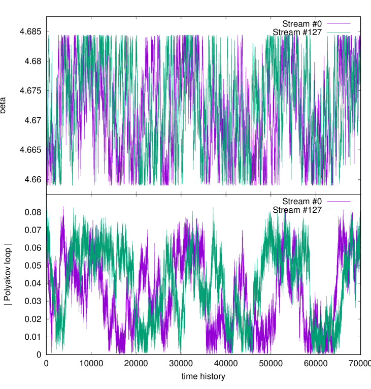
Figure 1: The $\beta$ history (above) and Polyakov loop average (below) of 2 streams as a function of the Monte Carlo sweeps in a simulation on a $45^{3}\times 10$ lattice with 128 streams on the range $4.659\leq\beta\leq 4.6844$ divided equidistantly.

To set up the simulations we need to choose the set of $\beta$ values we want to carry out simulations at. The distance between neighboring ensembles, $\Delta\beta$ needs to be small enough such that the acceptance of the swapping updates is $O(1)$ (see below for more details).

In Fig. 1 we show the $\beta$-history of two streams (out of 128) for a simulation on a $45^{3}\times 10$ lattice. As one observes the streams follow a trajectory similar to a random walk on the allowed $\beta$ range and they visit all points for a long enough simulation. This introduces correlations between ensembles at different $\beta$ values, which we will take into account later. As also visible on Fig. 1, the value of the Polyakov loop changes relatively slowly during the history of the stream. If we look at the history of the Polyakov loop for a given $\beta$, the largest autocorrelation comes from the instances when the same stream contributes (even if the stream visited other $\beta$ values in the meantime). We therefore reorder the Monte Carlo chain using the stream ID number of the contributions (and keep the chronological order among contributions from each stream). This ensures that the most correlated contributions will be close to each other (i.e., this ordering results in the largest autocorrelation for the given Monte-Carlo chain), which helps to minimize the correlations between blocks in the jackknife analysis. In Fig. 2 we show the resulting autocorrelation function for several lattice sizes at $\beta=4.5095$, compared with autocorrelation functions of brute force simulations. In the left panel of Fig. 3 we show the measured autocorrelation times for various simulation setups. As one observes the autocorrelation is substantially smaller for the parallel tempering simulations, although at the increased cost of having to simulate at all $\beta$ values. Therefore a fairer comparison would consider several brute force simulations at all $\beta$ values. In the right panel of Fig. 3 we show the number of statistically independent configurations created in brute force and in parallel tempering simulations at similar parameters, using the same amount of computational resources. We observe that $\tau_{PP}$, the autocorrelation time of the Polyakov loop also improves greatly as the number of $\beta$ values increases in a given $\beta$ range and as $\Delta\beta$ decreases (increasing the acceptance rate of swap updates). From the red and black points in Fig. 3, we see that the number of independent configurations created by the tempering algorithm increases substantially by simply decreasing $\Delta\beta$. Increasing the density of $\beta$ values, as between the red and blue points, results in nearly the same efficiency, indicating that the decrease in the number of updates (due to having twice as many streams for the same computer time) scales roughly with the decrease in the autocorrelation time.

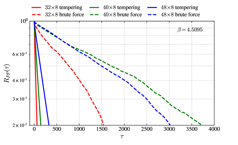
Figure 2: The autocorrelation function of the absolute value of the Polyakov loop at $\beta=4.5095$ for the lattice sizes $32^{3}\times 8,\ 40^{3}\times 8,\ 48^{3}\times 8$, in a parallel tempering simulation (solid lines), using 64 $\beta$ values with spacings $\Delta\beta=0.001$, and in single simulations (dashed lines).

Figure 3: (Left) The autocorrelation time of the Polyakov loop as a function of $\beta$ for simulations on a $32^{3}{\times}8$ lattice computed using the tempering algorithm (solid points) and using the brute force method (unfilled points) around the transition temperature for $N_{t}=8$ with equal amounts of computer time. The number of $\beta$ values and their spacing, $\Delta\beta$, are given for each simulation. $\tau_{PP}$ is improved by about an order of magnitude due to the stream-swapping of the tempering algorithm compared to that of the brute force approach. $\tau_{PP}$ also improves greatly as the number of $\beta$ values increases (increasing the number of participating streams at any given $\beta$) and as $\Delta\beta$ decreases (increasing the probability of any one stream being swapped). (Right) The efficiency of each simulation in terms of the number of computed updates divided by the autocorrelation time.

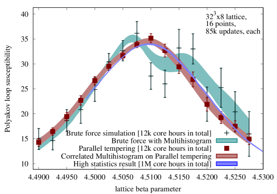
Figure 4: The susceptibility of the Polyakov loop average Eq. (5) measured on a $32^{3}\times 8$ lattice with several different algorithms and analyses as indicated, using 12k core hours of computer time. One local update step consists of three complete sweeps of overrelaxation and one heatbath step at each site and each of the three SU(2) subgroups. On the $32^{3}\times 8$ lattice the full local update completes in $0.64$s on a 68-core KNL card. A high statistics result is also shown for comparison.

Finally, in Fig. 4 we show one of the observables of interest: the Polyakov loop susceptibility. We show results from parallel tempering and brute force simulations using the same amount of computational resources. For comparison we also show the “correct” result we calculated using much larger statistics. We observe that the parallel tempering simulations give much smaller statistical errors. Although the brute force simulations are normally analyzed with the multihistogram method [34], we see that the parallel tempered simulations are superior to that as well. Moreover, one can also use the multihistogram method for the results of the parallel tempering algorithm, for a slight reduction of its errors, as most of the benefit of information of nearby ensembles is gained already using the swapping updates. As the parallel tempering introduces correlations between ensembles at different $\beta$s, the multihistogram analysis becomes slightly more complicated (see in Appendix A). In fact, the multihistogram algorithm is based on a linear combination of the reweighted results of all the available ensembles to minimize statistical errors. Therefore, if we use the uncorrelated multihistogram procedure on the parallel tempered ensembles, we might get slightly larger error bars, as we use a suboptimal linear combination. In practice, the correlations between ensembles are quite small, neglecting these correlations in the multihistogram procedure causes a negligible change in the results (much smaller than the statistical errors).

To summarize, we find the usage of the parallel tempering algorithm is very beneficial in these investigations. A multihistogram analysis helps to further reduce the statistical errors only slightly, as most of the effect of the swap updates is present already in the single $\beta$ ensembles.

III Transition Temperature

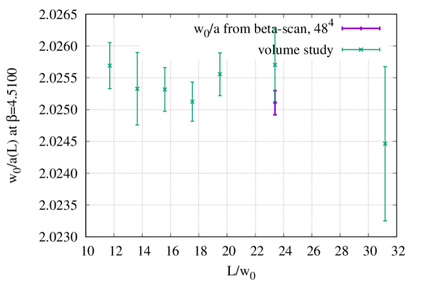
Figure 5: Volume dependence of the $w_{0}$ scale. $w_{0}/a$ is computed using fixed bare quark masses that correspond to the physical point, and is shown as a function of the spatial extent of the box in lattice units $L/w_{0}$. Fluctuations are comparable to the statistical error at each volume in the study; hence, finite-volume effects remain small.

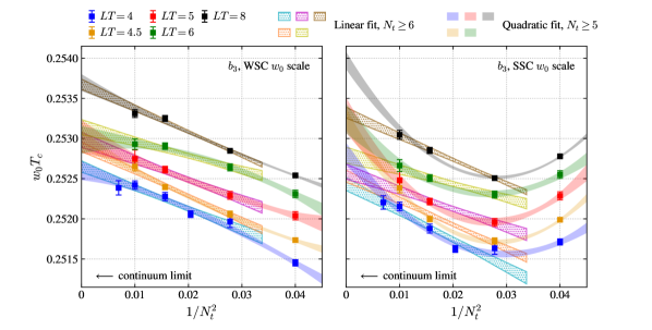
Figure 6: Two example plots that summarize the continuum extrapolation of the transition temperature $w_{0}T_{c}$ computed from the zero-crossing of $b_{3}$ at five fixed lattice aspect ratios $LT$; the zero-crossing is converted into the quantity $w_{0}T_{c}$ using (Left) the WSC $w_{0}$ scale and (Right) the SSC $w_{0}$ scale. Each data point is the median value of $w_{0}T_{c}$ computed for that lattice from the systematic analysis, and the error bars give the combined statistical and systematic error. Error bands are shown for the two kinds of extrapolating fit that are used: a linear fit to lattices with $N_{t}\geq 6$, and a quadratic fit to lattices with $N_{t}\geq 5$. The error bands give the combined statistical and systematic error from all similar fits performed in the analysis.

Figure 7: A summary plot of the infinite volume extrapolation of the continuum transition temperature $w_{0}T_{c}$ computed (Left) from the zero-crossing of $b_{3}$ and (Right) from the peak of $\chi_{R}$. Each point is the median value of $w_{0}T_{c}$ computed for each aspect ratio $LT$ in the systematic analysis, and the error bars give the combined statistical and systematic error. Error bands are shown for the quadratic fit to $LT\geq 4$. The error bands give the combined statistical and systematic errors from all similar fits in the analysis. The extrapolations from $b_{3}$ and $\chi_{R}$ are in agreement, as expected. The final result, $w_{0}T_{c}=0.25384(23)$, is shown in green.

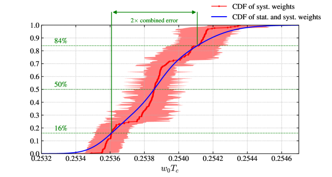
Figure 8: The cumulative distribution function (CDF) of all the results from the systematic analysis of the infinite volume limit of $w_{0}T_{c}$ in the continuum. The red curve shows the central value for each analysis, and the error band shows the statistical error. The blue curve gives the synthesized CDF defined in Eq. (11) combining the statistical and systematic errors. The final result is $w_{0}T_{c}=0.25384(23)$.

A well-defined transition temperature can be established using a variety of observables that are moments of the order parameter, which for pure ${\rm SU}(3)$ theory is the Polyakov loop $P$. In the analysis of this section, we extract the transition temperature using two of these observables: the susceptibility of the Polyakov loop,

$$\chi=N_{s}^{3}\left(\langle|P|^{2}\rangle-\langle|P|\rangle^{2}\right),$$ (5)

and the third-order Binder cumulant of the Polyakov loop,

$$b_{3}=\frac{\langle|P|^{3}\rangle-3\langle|P|\rangle\langle|P|^{2}\rangle+2\langle|P|\rangle^{3}}{\left(\langle|P|^{2}\rangle-\langle|P|\rangle^{2}\right)^{3/2}}.$$ (6)

At finite volume, the susceptibility as a function of the coupling $\beta$ shows a peak around the transition temperature. The value of the coupling at which the peak occurs, which we call $\beta_{\chi}$, approaches a value $\beta_{c}$ in the infinite volume limit as the height of peak diverges linearly with the volume and the width of the peak goes to zero linearly with the inverse volume; this value corresponds to the transition temperature. $b_{3}$ is used in an analogous fashion: as an odd central moment of the order parameter, instead of a peak, $b_{3}$ has a zero-crossing at a particular coupling value which we call $\beta_{b}$. The slope of $b_{3}$ around the zero-crossing increases linearly with the volume. In the infinite volume limit, the zero-crossing of $b_{3}$ becomes a jump-discontinuity at the phase transition, and $\beta_{b}$ approaches the same value of the critical couplings as does $\beta_{\chi}$.

If one wants to compare results at different lattice spacings, the susceptibility defined in Eq. (5) should be renormalized when one extracts $\beta_{\chi}$ [47]. The zero-crossing of $b_{3}$ is clearly unaffected by scaling, so $b_{3}$ does not need to be renormalized when extracting $\beta_{b}$. For every lattice, we renormalize the bare susceptibility as

$$\chi_{R}(\beta,N_{s},N_{t})=Z^{N_{t}}(\beta)\,\chi(\beta,N_{s},N_{t}),$$ (7)

where $N_{t}$ is the temporal extension of that lattice, with the renormalization condition that

$$\chi_{R}(\beta_{b},4N_{t},N_{t})=Z^{N_{t}}(\beta_{b})\,\chi(\beta_{b},4N_{t},N_{t})=1,$$ (8)

i.e. we fix $\chi_{R}(\beta_{b})=1$ for all lattices with aspect ratio $LT=N_{s}/N_{t}=4$. $\beta_{b}$ is used in the renormalization condition because, as just mentioned, it is a scale-invariant quantity. Because the normalization function $Z(\beta)$ is itself $\beta$-dependent, the location of the peak of $\chi_{R}(\beta)$ differs slightly from that of $\chi(\beta)$; hence, $\beta_{\chi}$ is dependent on the renormalization. Obviously, it is not strictly necessary to renormalize the susceptibility in order to extract $\beta_{c}$. As the width of the bare peak decreases linearly with the inverse volume, $Z(\beta)$ becomes approximately constant across that width, and so the difference between $\beta_{\chi}$ of $\chi(\beta)$ and $\beta_{\chi}$ of $\chi_{R}(\beta)$ should go to zero in the infinite volume limit. Thus, the value of $\beta_{c}$ extracted from $\chi(\beta)$ should agree with the value of $\beta_{c}$ extracted from $\chi_{R}(\beta)$. However, that our results may be formally correct and to avoid any potential ambiguities, we use the renormalized susceptibility in this analysis.

We extract $\beta_{\chi}$ and $\beta_{b}$ by fitting $\chi_{R}(\beta)$ and $b_{3}(\beta)$ in the vicinity of the peak and of the zero-crossing respectively. We employ basic polynomial fits of degrees 3, 4, 5, and 6. As a consequence of the stream-swapping in the tempering algorithm, correlations exist in the Polyakov loop data computed at different values of $\beta$ for a given lattice (see Sec. II for details); thus, correlations also exist among each moment of the Polyakov loop computed at different $\beta$ for each lattice. Therefore, we use the well-established practice of fitting with correlations using a subspace of the covariance matrix. The essential details are as follows. When fitting either $\chi_{R}(\beta)$ or $b_{3}(\beta)$ for a particular lattice, the covariance matrix of the fitted quantity is computed and diagonalized. In the diagonalized matrix, the smallest eigenvalues are averaged over and replaced with that average. After the averaging, the covariance matrix is converted back to its original basis. The cutoff for what counts as a small eigenvalue is freely chosen. We consider three choices for the cutoff: 10%, 5%, and 1% of the largest eigenvalue. For completeness and comparison, we also consider an uncorrelated fit. Ultimately, whether one uses a correlated fit or no correlation at all, we find that it makes very little difference on the final result for the transition temperature (see the error budget). In order to be able to interpret the $\chi^{2}$ of the fit to $\chi_{R}(\beta)$ or $b_{3}(\beta)$, one can use a correlated fit. The final result for the critical couplings including combined systematic and statistical errors are included in App. B.

To extrapolate $\beta_{\chi}$ and $\beta_{b}$ to the continuum and infinite volume limits to get $\beta_{c}$, we use the following set of lattice parameters:

$N_{t}$	$N_{s}$
5	15, 20, 22*, 23*, 25, 30, 40
6	18, 21, 24, 27, 30, 36, 48
7	28
8	24, 28, 32, 36, 40, 48, 64
10	30, 35, 40, 45, 50, 60, 80
12	48

The volumes are chosen such that there are lattices with aspect ratios $LT=3$, 4, 4.5, 5, 6, and 8, for $N_{t}=5$, 6, 8, and 10 (to obtain data at $LT=4.5$ for $N_{t}=5$, we find $\beta_{\chi}$ and $\beta_{b}$ for the lattices $22^{3}{\times}5$ and $23^{3}{\times}5$ and then interpolate linearly in $1/N_{s}^{3}$ to get $\beta_{\chi}$ and $\beta_{b}$ for a hypothetical “$22.5^{3}{\times}5$” lattice), and that there are lattices with $LT=3.5$ for $N_{t}=6$, 8, and 10. Two additional lattices of $LT=4$ are also chosen for $N_{t}=7$ and 12.

Now, the value of the coupling $\beta$ is specific to the choice of action on the lattice; hence, while $\beta$ is useful for comparing results computed using the same action, it must be translated into a physically meaningful quantity, the lattice temperature $T$, to yield results that are independent of the choice of action. This requires the use of a scale setting. We use the $w_{0}$ scale based on the Wilson flow, implicitly defined by

$$t\frac{d}{dt}\left[t^{2}E(t)\right]_{t=w_{0}^{2}}=0.3,$$ (9)

where $E(t)$ is the expectation value of the gauge action of lattice configurations evolved via the Wilson flow [48, 49]. We compute the $w_{0}$ scale in lattice units, $w_{0}/a$, for many values of $\beta$ for two different discretisations of the flow (WSC and SSC in the notation of [50]). This gives us another systematic choice as to which version of the scale setting to use. We then interpolate these results to get $w_{0}/a(\beta)$ by fitting with a polynomial of order 6 and 7 in the $\beta$ range [4.0,4.95]. It is critical to ensure that finite-volume effects on the $w_{0}$ scale remain small, as these effects increases with the flow time [48]. In Fig. 5, we present a volume study of the $w_{0}$ scale (WSC) computed in this analysis. Fluctuations in $w_{0}/a$ are comparable in size to the statistical error at each volume; consequently, no significant volume dependence can be seen.

Once $w_{0}/a(\beta)$ is found for a particular $\beta$ on a lattice with a temporal extension of $N_{t}$, it can be converted into the lattice temperature $T=(N_{t}a)^{-1}$ by dividing by $N_{t}$:

$$\frac{w_{0}}{aN_{t}}=w_{0}T.$$ (10)

In this way, $\beta_{\chi}$ and $\beta_{b}$ are converted into the dimensionless quantity $w_{0}T_{c}$ for each lattice.

To compute the continuum value of the transition temperature $w_{0}T_{c}$ at infinite volume, we first find the continuum value of $w_{0}T_{c}$ at finite volume and fixed lattice aspect ratio $LT=N_{s}/N_{t}$ and then extrapolate the results of the continuum theory at different $LT$ to the limit where $(LT)^{3}\rightarrow\infty$. That a continuum limit for $w_{0}T_{c}$ exists for pure ${\rm SU}(3)$ at finite volume is not immediately obvious; however, as shown in Fig. 6, a well-defined continuum value of $w_{0}T_{c}$ can in fact be established at fixed aspect ratio $LT$ using both definitions for $\beta_{c}$. We use large lattices with aspect ratios $LT=4$, 4.5, 5, 6, and 8 for four different temporal extensions: $N_{t}=5$, 6, 8, and 10. To check the consistency of the continuum extrapolation at other temporal extensions, we also include two lattices with $N_{t}=7$ and 12 in the $LT=4$ extrapolation. In the left panel of Fig. 6, one can see that $w_{0}T_{c}$ goes roughly linearly with $N_{t}^{-2}$ for each $LT$. We perform two types of fit to extrapolate to the continuum: a linear fit to all lattices with $N_{t}\geq 6$, and a quadratic fit to all lattices with $N_{t}\geq 5$. The fits are shown in Fig. 6; the error bands give the combined statistical and systematic errors from all the similar fits performed in the analysis.

The continuum results from $\chi_{R}$ and $b_{3}$ are shown in Fig. 7 as functions of $(LT)^{-3}$, which behaves as the inverse volume. A quadratic fit to $LT\geq 4$ is used to extrapolate to the infinite volume limit. This fit is shown in Fig. 7 for both $\chi_{R}$ and $b_{3}$. The error bands give the combined statistical and systematic errors from all the similar fits that were performed. We find that the infinite volume value of the transition temperature $w_{0}T_{c}$ computed using $\chi_{R}$ agrees with the value computed using $b_{3}$, as expected.

Following the analysis method introduced in [51] to estimate the statistical and systematic uncertainties of the results, in total we have performed 256 different analyses, these are characterized by the choice of the moment of the Polyakov loop ($\chi_{R}$ or $b_{3}$), the degree of the fit to the moment (3, 4, 5, or 6), whether and how the fit is correlated (uncorrelated or correlated with an eigenvalue cutoff of 10%, 5%, 1%), the choice of the $w_{0}$ scale calculation (WSC, SSC), the degree of fit to the $w_{0}$ scale data (6 or 7), and the degree and range of the continuum extrapolation (linear or quadratic). The cumulative distribution function (CDF) of the infinite volume results of these analyses is shown in Fig. 8 in red, where the central value and statistical error of each result are given. The statistical and systematic uncertanities are synthesized into a smooth CDF defined by the equation

$$F(w_{0}T_{c})=\frac{1}{2}+\frac{1}{2\cdot 256}\sum_{i=1}^{256}w_{i}\,{\rm erf}\left(\frac{w_{0}T_{c}-\mu_{i}}{\sqrt{2}\sigma_{i}}\right)$$ (11)

where $\mu_{i}$ and $\sigma_{i}$ are the central value and statistical uncertainty respectively of the $i$th analysis, and $w_{i}$ is the weight of the CDF of the $i$th result. (This equation then assumes that the statistical result of each analysis is well-described by a normal distribution with a mean of $\mu_{i}$ and standard deviation of $\sigma_{i}$.) We have no prior assumptions as to the relative statistical significance of any of the analyses, and so we take an agnostic position by weighting all analyses equally, i.e. by setting $w_{i}=1$. The result is shown in blue in Fig. 8. The final result is then the median value of the smooth CDF, implicitly defined by $F(w_{0}T_{c})=0.5$, and the central 68% width is taken as twice the total error. This yields a final value of $w_{0}T_{c}=0.25384(23)$, which is shown in green in Fig 7, with an error budget of median 0.25384 statistical error 0.00011 0.043 % full systematic error 0.00021 0.082 % Observable ($b_{3}$ , $\chi_{R}$) $1.1\cdot 10^{-5}$ 0.0042 % Fit order (3, 4, 5, 6) $2.1\cdot 10^{-5}$ 0.0085 % Fit type (corr, uncorr) $1.2\cdot 10^{-5}$ 0.0047 % Scale setting (WSC, SSC) $1.9\cdot 10^{-5}$ 0.0075 % Scale fit order (6, 7) $2.4\cdot 10^{-6}$ 0.0010 % Continuum limit range $1.2\cdot 10^{-4}$ 0.0487 %

IV Evidence for a first order transition

In this section we use our simulations to demonstrate that the thermodynamic transition of the SU(3) Yang-Mills theory is first order, as anticipated. We can perform this in two ways.

First we study the finite volume scaling of the susceptibility (scaled variance) of the order parameter. As we did in the case of the transition temperature study, we again use the susceptibility ($\chi_{R}$) of the renormalized Polyakov loop. If the transition is of first order, the leading volume dependence must be $\chi_{R}^{-1}\sim V^{-1}$. Such a study would not be new and also would not give a true evidence, if we used data from a fixed lattice resolution. Here we first calculate the continuum limit of the peak height for various volumes, and then demonstrate the expected volume scaling. Moreover, we show the continuum extrapolation of $\chi_{R}$ as a function of $w_{0}T$ around the critical value $w_{0}T_{c}$, and display the expected volume dependence.

Perhaps the most convincing argument for the first order nature of a transition is the existence of a latent heat in the thermodynamic and continuum limit. Here we are building on the work of the WHOT collaboration [52, 44]. Aided by the tempering algorithm and the improved action we arrive at a combined continuum and infinite volume limit, 29 standard deviations away from zero.

IV.1 Finite volume scaling of the Polyakov loop susceptibility

The obtain the finite volume scaling of a susceptibility, it has to be continuum extrapolated for several fixed physical volumes. This raises the question of renormalization, a topic that one could ignore as long as only one lattice resolution is relied upon. As discussed before, $\chi_{R}(L,T)=Z^{N_{t}}(\beta)\chi(\beta,N_{x},N_{t})$ with $L=a(\beta)N_{x}$ and $T^{-1}=a(\beta)N_{t}$. The renormalization condition for $Z$ is defined at a fixed volume, for us the choice is $LT=4$ (meaning $N_{x}=4N_{t}$). Scanning through the resolutions $N_{t}=4,5,6,7,8,10,12$ and setting the renormalization condition $\chi_{R}(L=4T_{c}^{-1},T=T_{c})\equiv 1$ one can easily obtain $Z(\beta)$ for the whole range of interest. Clearly, in this setting we lose any information about an overall constant in $\chi_{R}$, but being this a volume independent factor, the actual finite size scaling is left intact.

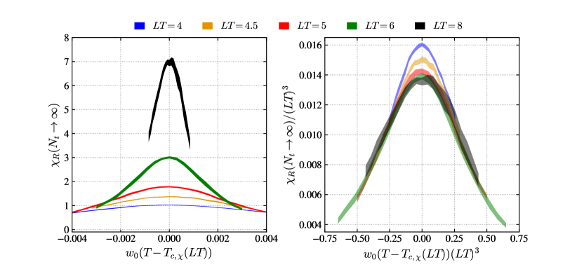
Figure 9: (Left) The continuum extrapolated renormalized Polyakov loop susceptibility at different volumes, centered around the volume-dependent peak position $w_{0}T_{c,\chi}(LT)$. The bands include both statistic and systematic uncertainties. (Right) Same curves as in the left panel, but scaled with appropriate powers of the volume, in order to highlight the linear volume dependence typical of a first order transition.

We select fixed physical volumes ($LT=4.5,5,6,8$) and interpolate $Z(\beta)$ to the actual volume dependent $\beta_{c}$ of each simulation with $N_{t}=5,6,8$ and 10. The renormalized result $\chi_{R}(L,T)=Z^{N_{t}}(\beta)\chi(\beta,N_{x},N_{t})$ is simply continuum extrapolated as $N_{t}^{2}$. Such continuum extrapolation is shown in Fig. 9 for the $\chi_{R}(w_{0}T)$ curves at fixed volume, and in Fig. 10 for the inverse peak height. In Fig. 9 (left), each curve is continuum extrapolated at the indicated fixed volume, and the bands include both statistic and systematic uncertainties. Note that, had we subtracted the infinite volume limit value $\chi_{R}(w_{0}T_{c})$ instead of the volume-dependent peak values $\chi_{R}(w_{0}T_{c,\chi}(LT))$, the curves would not have have been exactly centered around zero, but a trend would have appeared where larger volumes would peak closer to zero. However, as can be seen in the right panel of Fig. 7, the difference would be negligible, since the continuum extrapolated peak position shows a very mild volume dependence. The right panel shows the same curves, but scaled with the volume in order to highlight the volume dependence. We can see that the bands corresponding to $LT=5,6,8$ are overall almost indistinguishable, clearly showing that they fall in the linear volume scaling regime typical of a first order transition.

In Fig. 10 we actually show two extrapolations, one for each definition of $T_{c}$, using the zero of the 3rd Binder cumulant or the susceptibility peak in red and blue, respectively. The extrapolations do not differ at all depending on this ambiguity, the main systematic uncertainty comes from the possibility to include a inverse quadratic volume term in the infinite volume extrapolations. We find that the inverse susceptibility is extrapolated to be vanishing, (or, actually, strongly constrained: $\chi_{R}^{-1}(V=\infty)=0.0023(58)_{\rm stat}(65)_{\rm sys}$ ) in the infinite volume limit. (A crossover transition is signaled by a positive value of the infinite volume extrapolated inverse susceptibility).

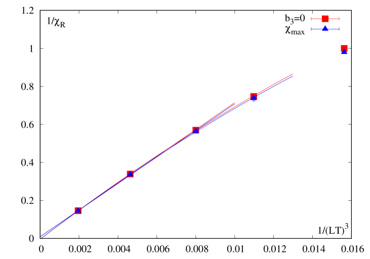
Figure 10: Infinite volume extrapolation of the inverse Polyakov loop susceptibility. The results are renormalized and continuum extrapolated, systematic errors are included. The renormalization condition was $\chi_{R}(L=4T_{c}^{-1},T_{c})=1$. We use red symbols if we defined $T_{c}$ though the zero of the third Binder cumulant, blue symbols when we defined $T_{c}$ as the peak of the susceptibility. Depending on the details of the infinite volume extrapolation we get a slightly positive or negative result. All in all we get the result $\chi_{R}^{-1}(V=\infty)=0.0023(58)_{\rm stat}(65)_{\rm sys}$ The linear scaling sets in for $LT\geq 5$. The linear convergence of $\chi_{R}^{-1}$ to zero indicates a first order transition.

IV.2 Calculation of the latent heat

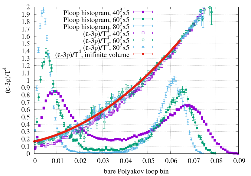
Figure 11: We show the Polyakov loop histograms for three volumes ($N_{t}=5$) along with the trace anomaly expectation values for each Polyakov loop bin. The double peak structure and the sharpening of the peaks with increasing volume match our expectations for a first order transition. The trace anomaly shows no discontinuity in this representation, the infinite volume limit can be found using a polynomial model.

A non-vanishing latent heat identifies a transition to be first order beyond doubt. Its calculation, however, is much less trivial than observing a transition peak in a susceptibility. Most conveniently, the latent heat can be understood as the discontinuity of the trace anomaly, $(\epsilon-3p)/T^{4}$, as the transition is crossed. This assumes a continuous pressure, which is assumed in all transition scenarios. The difficulty in quantifying this gap arises from two sources:

a) To calculate a discontinuity one must get very close to $T_{c}$ from both sides. The trace anomaly happens to have a pronounced temperature dependence just above and just below $T_{c}$.

b) The trace anomaly has a quartic divergence, thus brute force statistics must scale with $\sim N_{t}^{8}$ to compensate. Even in quenched QCD, this can quickly become the driving factor in the costs for $N_{t}\geq 8$.

When the continuum limit is desired, point b) determines the amount of statistics needed, but point a) must be addressed in all cases. Just “reading off the jump” could give any value between zero and 2 for $\Delta(\epsilon-3p)/T_{c}$ as shown in Fig. 1 of our earlier study [53]. One could define the latent heat as the surface under the peak of the energy susceptibility, however, the signal-to-noise ratio is diminishing in the infinite volume limit.

The most successful method to define the latent heat, the one we also use here, is to simulate right at $\beta_{c}$ and classify the lattice configurations into the cold and hot phases (see Refs. [52, 44]). The trace anomaly can then be evaluated for both the hot and cold halves of the ensemble, the difference gives the latent heat up to a renormalization factor. The absolute value of the Polyakov loop shows a clear double peaked histogram. Selecting the Polyakov loop magnitude at the minimum of this histogram between the two peaks as the cut value, we introduce a phase categorization which has a systematic error decreasing exponentially with growing volume. This criterion works well on smeared (flowed) configurations as well [44].

We illustrate this approach on our $N_{t}=5$ ensembles at $\beta_{c}$. We reweighted our closest $\beta$-ensemble to the point where $b_{3}(\beta)=0$ for the particular simulation volume. The bare Polyakov loop histograms are shown in Fig. 11 for three of our simulation volumes. We show the standard jackknife errors on the histograms. For this lattice spacing we could reach an aspect ratio of $LT=16$, where the separation of the two peaks are very clear, indeed. Yet even near the minimum we have enough hits in the Polyakov loop bins to quantify the trace anomaly bin by bin.

The trace anomaly shows no discontinuity between the phases, its Polyakov loop dependence can be modeled by a polynomial. In Fig. 11 we fit a 3rd order polynomial with finite volume corrections proportional to $1/L^{3}$ to obtain the infinite volume extrapolation (red curve). This picture connects the latent heat with the hot-phase value of Polyakov loop. The cold phase peak moves to zero as $1/L^{3}$, hence, the $y-$intercept of the red curve points to the trace anomaly at $T_{c}-\epsilon$. Similarly, the non-trivial position of second histogram peak in the thermodynamic limit is translated by the same curve to the trace anomaly at $T_{c}+\epsilon$.

As observed in Fig. 11, one may define the latent heat at a fixed ensemble, by translating the peak positions into a pair of trace anomaly values through the red curve (the infinite volume extrapolation of the trace anomaly as function of the magnitude of the Polyakov loop), and than taking the difference. While this is clearly possible, it is to be seen in practice, if the volume scaling turns linear in $1/L^{3}$ for practical lattice sizes. Alas, this is not the case. Both the peak positions and the trace anomaly they relate to, are heavily non-linear in the range $4\leq LT\leq 8$, where most of our statistics is collected. However, integrating the trace anomaly curve with the histogram peak’s weight for both peaks gives a linear result. This is then equivalent to the approach in Ref. [52] where the trace anomalies were simply averaged for both cold and hot sub-ensembles. In summary, we first define a cut value in the modulus of the Polyakov loop for each lattice size individually as the minimum position of the discussed histogram. These bins play no role in the second step, where we calculate the trace anomaly for the configurations above and below this cut, separately. The trace anomaly difference between these two sub-ensembles gives the latent heat normalized to $T^{4}$.

Let us now come to point b). Ref. [44] introduces a truly innovative way to separate the UV noise of the physics result in the trace anomaly. The results are calculated at small gradient flow time, where the square root of the flow time replaces the lattice spacing in its role as a cut-off scale. The presence of a small, physical flow time eliminates the quartic divergence and the continuum limit can be taken. Using larger flow time allows the usage of coarser lattices. This then needs to be related to the real theory at zero flow time using small flow time expansion [54], which gets harder as the selected flow time increases.

In this study, we analyzed the configurations at zero flow time directly. To mitigate the quartic divergence, we used the tree-level Symanzik improved action. This choice does not improve the quartic scaling of the simulation noise, yet it endorses coarser lattices within the linear range continuum scaling. We use lattices up to $N_{t}=10$ instead of the $N_{t}=16$ of Ref. [44], this immediately allows for simulating a factor $43\approx(16/10)^{8}$ less statistics due to the quartic divergence of the trace anomaly. (This factor must be considered together with the fact that the improved action comes at a 2.1 times higher cost.)

The trace anomaly in Fig. 11 was renormalized using the standard scheme of Ref. [56]

$$\frac{\epsilon-3p}{T^{4}}=N_{t}^{4}a\frac{d\beta}{da}\left(\left\langle S_{g}\right\rangle_{N_{s}^{3}\times N_{t}}-\left\langle S_{g}\right\rangle_{\mathrm{infinite}~{}N_{t}}\right)\,,$$ (12)

where $S_{g}$ is the gauge action without the factor of the inverse coupling $\beta$. The logarithmic derivative of the $\beta$ – lattice spacing ($a$) relation was obtained using our $w_{0}$ scan, the same that already used as high precision scale setting in Section III. The same runs were used to calculate the zero temperature gauge action $\left\langle S_{g}\right\rangle_{\mathrm{infinite}~{}N_{t}}$, that is not necessary for latent heat itself, only if one is interested in trace anomalies at $T_{c}\pm\epsilon$.

We calculated the trace anomaly differences for the ensembles that we generated. We find that a combined linear continuum and infinite volume fit is possible and thus we get the result in Fig. 12.

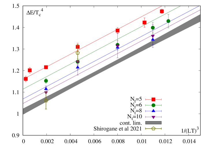
Figure 12: Combined and continuum limit of the trace anomaly difference between the hot and cold phases. The extrapolation is linear both in $1/N_{t}^{2}$ and $1/L^{3}$, in this example we exclude all ensembles with $N_{t}<6$ or $LT<5$. The continuum extrapolated but finite volume results in Ref. [44] are shown for comparison.

For the final results we consider the following sources of systematic uncertainties. The continuum limit is calculated both using and not using $N_{t}=5$, including or not including the aspect ratio $LT=4.5$ into the infinite volume extrapolation. We use various number of Polyakov bins (100, 200 or 400) and two different log-polynomial models for fitting the negative logarithm of the histogram so that cut value separating the phases can be calculated. We have performed two separate analyses: first using reweighting to $\beta_{c}$ from the closest available $\beta$ ensemble, second, using the multihistogram method to calculate averages at $\beta_{c}$. In the end we obtain

$$\Delta\left[\frac{\epsilon-3p}{T^{4}}\right]=1.025(21)_{\rm(stat)}(27)_{\rm(sys)}$$ (13)

with an error budget of

median	1.0249
statistical error	0.021	2.1 %
full systematic error	0.027	2.7 %
Histogram fitting	0.0030	0.29 %
Histogram binning	0.0002	0.02 %
$\beta_{c}$ definition	0.0135	1.32 %
$w_{0}$ interpolation	0.0007	0.07 %
$LT$ range	0.0121	1.18%
$N_{t}$ range	0.0157	1.53%
Analysis method	0.0019	0.18%

V Conclusion

In this paper we have studied the phase transition in an SU(3) pure gauge theory. First we have investigated the efficiency of parallel tempering simulations to measure properties of the system near the phase transition point. The parallel tempering allows swap updates between simultaneous calculations at different temperatures. One observes a sizable decrease of the autocorrelation times compared to simulations at a fixed temperature. As observed the efficiency of parallel tempering is superior to even brute force simulations using multihistogram analysis to combine the data of all the ensembles.

Next we have determined the critical temperature of the theory. We used two definitions to find the transition point: the peak of the Polyakov loop susceptibility and the zero of the 3rd Binder cumulant of the Polyakov loop. The ensembles in this study consisted of lattices with temporal lattice size $N_{t}=5,6,8,10$ and 12 with aspect ratios $LT=4,4.5,6,8,10,12$, using the Symanzik gauge action. First, we carried out a continuum extrapolations for fixed aspect ratios, giving the continuum extrapolated critical temperatures for finite physical volumes. Second we calculated the infinite volume extrapolated critical temperatures, and and observed the coincidence of the two definitions extrapolated to the thermodynamic limit in the continuum, as expected. The systematic errors of the calculation were thoroughly investigated by exploring many possible fitting and extrapolation procedures. Our final result for the critical temperature with combined statistical and systematic error is: $w_{0}T_{c}=0.25384(23)$.

Finally we have investigated the properties of the phase transition. We have confirmed the first order nature of the transition by first investigating the finite volume scaling of the peak of the Polyakov loop susceptibility. For this we have calculated the continuum limit of the renormalized Polyakov loop susceptibility for different physical system sizes. As one observes both the height and the width of the susceptibility follow the appropriate scaling in the infinite volume limit, confirming that the phase transition is first order. Second, we have calculated the latent heat of the transition, with the help of the discontinuity of the trace anomaly. The discontinuity was measured for each ensemble by averaging the trace anomaly at the critical coupling for “hot” and “cold” configurations, where the classification is based on the value of the Polyakov loop. Finally we carried out a combined infinite volume and continuum extrapolation, yielding the value $\Delta\epsilon/T_{c}^{4}=1.025(21)(27)$.

The tempering algorithm is not limited to quenched QCD. The same first order transition and the corresponding critical end-point can be addressed using tempering updates in gauge coupling in the heavy quark region [18]. Introducing pseudofermions the tempering updates can be extended to mass, imaginary chemical potential or other parameters of the fermionic action. This algorithm will probably play an important role in the exploration of the QCD phase diagram.

Acknowledgments The project received support from the BMBF Grant No. 05P21PXFCA. The authors gratefully acknowledge the Gauss Centre for Supercomputing e.V. (www.gauss-centre.eu) for funding this project by providing computing time on the GCS Supercomputer HAWK at HLRS, Stuttgart. Part of the computation was performed on the QPACE3 funded by the DFG and hosted by JSC and on the cluster at the University of Graz. S.B. thanks Julius Kuti for discussions on the topic.

Appendix A Correlated Multihistogram

Here we adopt the well known reweighting method by Ferrenberg and Swendsen [34] and extend it to correlated data.
The weighted average $a$ of data sets $x_{i}$, $i=1,2,...,m$ can be calculated by minimizing

$$\chi^{2}=\sum_{i,j}^{m}(x_{i}-a)\left(C^{-1}\right)_{i,j}(x_{j}-a),$$ (14)

with $C^{-1}$ being the inverse covariance matrix [57]. The minimum is found for

$$a=\frac{\sum_{i,j=1}^{m}\left(C^{-1}\right)_{i,j}x_{j}}{\sum_{i,j=1}^{m}\left(C^{-1}\right)_{i,j}},$$ (15)

which has minimal fluctuations compared to other possible linear combinations.
Interpolating observables such as the Polyakov loop to a target coupling $\beta$ demands a precise knowledge of the partition function $Z(\beta)$ and thus of the density of states $W$.

$$Z(\beta)=\sum_{E}W(E)e^{-\beta E}$$ (16)

Since $W(E)$ does not depend on $\beta$ it can be estimated by the densities of states of the individual simulations $W_{i}(E)$ according to eq. (15). Thus $i$ labels the simulation at $\beta_{i}$ which is correlated with the other ones due to the $\beta$ tempering algorithm. The histograms of the energy $N_{i}(E)$ can be related to the density of states by

$$W_{i}(E)\frac{e^{-\beta_{i}E}}{Z(\beta_{i})}=\frac{N_{i}(E)}{n_{i}},$$ (17)

where $n_{i}$ is the total amount of entries of the histogram. In the same manner the exact density of states $W(E)$ is estimated by multiple simulations performed at the same coupling

$$W(E)=\frac{\overline{N_{i}}(E)Z(\beta_{i})}{n_{i}e^{-\beta_{i}E}}.$$ (18)

It is important to note that $\overline{N_{i}}$ is the averaged histogram of these simulations, thus its error is $\sigma_{i}=\sqrt{g_{i}\overline{N_{i}}}$. The factor $g_{i}$ takes the correlation time $\tau_{i}$ of the ensemble into account and reads $g_{i}=1+2\tau_{i}$. The covariance for a certain energy $E$ between the densities of states of individual simulations $W_{i}$ and $W_{j}$ can be calculated as

$$\mathrm{cov}(W_{i},W_{j})=W^{2}\frac{\mathrm{cov}(N_{i},N_{j})}{\overline{N_{i}}\;\overline{N_{j}}}=W^{2}\frac{\mathrm{corr}(N_{i},N_{j})g_{i}g_{j}}{\sigma_{i}\sigma_{j}}.$$ (19)

Here $\mathrm{cov}(N_{i},N_{j})$ and $\mathrm{corr}(N_{i},N_{j})$ stand for components of the covariance and correlation matrix respectively which are estimated according to the standard Jackknife resampling method.
With eq. (15) the estimator of the exact density of states $W(E)$ can be written as

$$W(E)=\frac{\sum_{i,j=1}^{m}\sigma_{i}\sigma_{j}(g_{i}g_{j})^{-1}\;\mathrm{corr}^{-1}(N_{i},N_{j})\;W_{j}}{\sum_{i,j=1}^{m}\sigma_{i}\sigma_{j}(g_{i}g_{j})^{-1}\;\mathrm{corr}^{-1}(N_{i},N_{j})}$$

$$=\frac{\sum_{i,j=1}^{m}(g_{i}g_{j})^{-1/2}\sqrt{\frac{n_{i}Z_{j}}{n_{j}Z_{i}}}e^{E(\beta_{j}-\beta_{i})/2}\;N_{j}(E)\;\mathrm{corr}^{-1}(N_{i},N_{j})}{\sum_{i,j=1}^{m}(g_{i}g_{j})^{-1/2}\sqrt{\frac{n_{i}n_{j}}{Z_{j}Z_{i}}}e^{-E(\beta_{i}+\beta_{j})/2}\;\mathrm{corr}^{-1}(N_{i},N_{j})}.$$ (20)

In some cases the correlation matrix is singular, caused by bins which only contain a few entries. Since these bins have a very small contribution to the end result of $W(E)$, we neglect the correlation of them with other bins. In the case of uncorrelated simulations the correlation matrix is the unity matrix and we get back to the standard Ferrenberg-Swendsen equation for the density of states

$$W(E)=\frac{\sum_{i=1}^{m}g_{i}^{-1}N_{i}(E)}{\sum_{i=1}^{m}g_{i}^{-1}\frac{n_{i}}{Z_{i}}e^{-\beta_{i}E}}.$$ (21)

Inserting eq. (20) in eq. (16) the partition functions $Z_{i}$ of the individual simulations can be calculated iteratively. Assuming constant auto-correlation times $\tau_{i}$ the $g_{i}$ factors are the same for every simulation. According to eqs. (20) or (21) they represent a constant factor for all $Z_{i}$ which can be dropped.

Appendix B Critical couplings

The critical couplings for the ensembles used in this study are listed in Table 1. The quoted errors are combined systematic and statistical errors for the $\beta_{c}$ values calculated using fitting as described in Sec. III. Note that the critical couplings calculated using the multihistogram analysis have no systematic error, as they are simply solutions of the eqs. $b_{3}(\beta_{b})=\partial_{\beta}\chi(\beta_{\chi})=0$).

Lattice	$\beta_{c}$ from $b_{3}$,fit	$\beta_{c}$ from $b_{3}$, multihist	$\beta_{c}$ from $\chi^{R}$,fit	$\beta_{c}$ from $\chi$,fit	$\beta_{c}$ from $\chi$, multihist
$15\times 5$	4.19667(15)	4.19676(13)	4.20246(73)	4.20019(46)	4.19996(16)
$20\times 5$	4.19855(9)	4.19858(8)	4.20048(47)	4.19987(14)	4.19998(10)
$22\times 5$	4.19917(5)	4.19915(6)	4.20050(28)	4.20020(9)	4.20020(6)
$23\times 5$	4.19926(9)	4.19930(9)	4.20073(13)	4.20040(12)	4.20026(9)
$25\times 5$	4.19995(11)	4.19996(11)	4.20084(21)	4.20064(16)	4.20069(11)
$30\times 5$	4.20056(11)	4.20052(10)	4.20103(13)	4.20095(13)	4.20090(10)
$40\times 5$	4.20112(3)	4.20110(4)	4.20126(6)	4.20123(3)	4.20123(4)
$18\times 6$	4.30962(39)	4.30986(41)	4.31706(116)	4.31412(97)	4.31324(60)
$21\times 6$	4.31081(33)	4.31090(29)	4.31470(72)	4.31325(53)	4.31319(33)
$24\times 6$	4.31210(19)	4.31190(12)	4.31434(28)	4.31355(28)	4.31361(12)
$27\times 6$	4.31233(9)	4.31230(12)	4.31389(16)	4.31350(14)	4.31347(12)
$30\times 6$	4.31291(13)	4.31290(15)	4.31402(19)	4.31376(17)	4.31374(16)
$36\times 6$	4.31379(11)	4.31373(10)	4.31427(17)	4.31415(10)	4.31417(10)
$48\times 6$	4.31432(3)	4.31432(5)	4.31447(4)	4.31445(3)	4.31447(5)
$24\times 8$	4.50511(26)	4.50506(24)	4.51309(77)	4.50954(47)	4.50936(38)
$28\times 8$	4.50633(23)	4.50639(20)	4.51191(46)	4.50980(43)	4.50964(37)
$32\times 8$	4.50756(14)	4.50758(13)	4.51060(34)	4.50965(19)	4.50964(12)
$36\times 8$	4.50788(6)	4.50795(7)	4.50985(7)	4.50934(9)	4.50936(8)
$40\times 8$	4.50846(9)	4.50847(10)	4.50985(16)	4.50951(12)	4.50952(11)
$48\times 8$	4.50929(10)	4.50930(9)	4.50996(12)	4.50982(11)	4.50982(9)
$64\times 8$	4.51028(7)	4.51024(7)	4.51048(8)	4.51046(8)	4.51041(7)
$30\times 10$	4.66673(71)	4.66695(68)	4.67641(231)	4.67065(160)	4.67175(182)
$35\times 10$	4.66990(24)	4.67002(30)	4.67634(44)	4.67382(35)	4.67362(43)
$40\times 10$	4.67099(12)	4.67098(14)	4.67421(47)	4.67299(25)	4.67306(20)
$45\times 10$	4.67166(13)	4.67159(15)	4.67371(22)	4.67309(15)	4.67318(19)
$50\times 10$	4.67188(30)	4.67199(31)	4.67295(54)	4.67253(52)	4.67267(43)
$60\times 10$	4.67244(19)	4.67259(21)	4.67326(29)	4.67314(28)	4.67318(25)
$80\times 10$	4.67365(10)	4.67364(11)	4.67389(12)	4.67386(11)	4.67383(12)
$48\times 12$	4.80980(17)	4.80980(17)	4.81303(48)	4.81199(20)	4.81205(26)

Table 1: Critical couplings calculated using the fitting method explained in Sec. III and by the multihistogram analysis.

References

- Hagedorn [1965] R. Hagedorn, Statistical thermodynamics of strong interactions at high-energies, Nuovo Cim.Suppl. 3, 147 (1965).
- Cabibbo and Parisi [1975] N. Cabibbo and G. Parisi, Exponential Hadronic Spectrum and Quark Liberation, Phys.Lett. B59, 67 (1975).
- Polyakov [1978] A. M. Polyakov, Thermal Properties of Gauge Fields and Quark Liberation, Phys.Lett. B72, 477 (1978).
- Aoki et al. [2006a] Y. Aoki, G. Endrodi, Z. Fodor, S. Katz, and K. Szabo, The Order of the quantum chromodynamics transition predicted by the standard model of particle physics, Nature 443, 675 (2006a), arXiv:hep-lat/0611014 [hep-lat] .
- Svetitsky and Yaffe [1982] B. Svetitsky and L. G. Yaffe, Critical Behavior at Finite Temperature Confinement Transitions, Nucl.Phys. B210, 423 (1982).
- Yaffe and Svetitsky [1982] L. Yaffe and B. Svetitsky, First Order Phase Transition in the SU(3) Gauge Theory at Finite Temperature, Phys.Rev. D26, 963 (1982).
- Wu [1982] F. Y. Wu, The Potts model, Rev. Mod. Phys. 54, 235 (1982), [Erratum: Rev.Mod.Phys. 55, 315–315 (1983)].
- Fischer et al. [2015] C. S. Fischer, J. Luecker, and J. M. Pawlowski, Phase structure of QCD for heavy quarks, Phys. Rev. D91, 014024 (2015), arXiv:1409.8462 [hep-ph] .
- Kashiwa et al. [2012] K. Kashiwa, R. D. Pisarski, and V. V. Skokov, Critical endpoint for deconfinement in matrix and other effective models, Phys. Rev. D 85, 114029 (2012), arXiv:1205.0545 [hep-ph] .
- Pisarski and Wilczek [1984] R. D. Pisarski and F. Wilczek, Remarks on the Chiral Phase Transition in Chromodynamics, Phys.Rev. D29, 338 (1984).
- Brown et al. [1990] F. R. Brown, F. P. Butler, H. Chen, N. H. Christ, Z.-h. Dong, et al., On the existence of a phase transition for QCD with three light quarks, Phys.Rev.Lett. 65, 2491 (1990).
- Cuteri et al. [2021] F. Cuteri, O. Philipsen, and A. Sciarra, On the order of the QCD chiral phase transition for different numbers of quark flavours, (2021), arXiv:2107.12739 [hep-lat] .
- Saito et al. [2011] H. Saito et al. (WHOT-QCD Collaboration), Phase structure of finite temperature QCD in the heavy quark region, Phys.Rev. D84, 054502 (2011), arXiv:1106.0974 [hep-lat] .
- Ejiri et al. [2019] S. Ejiri, S. Itagaki, R. Iwami, K. Kanaya, M. Kitazawa, A. Kiyohara, M. Shirogane, and T. Umeda (WHOT-QCD), End point of the first-order phase transition of QCD in the heavy quark region by reweighting from quenched QCD, (2019), arXiv:1912.10500 [hep-lat] .
- Kiyohara et al. [2021] A. Kiyohara, M. Kitazawa, S. Ejiri, and K. Kanaya, Finite-size scaling around the critical point in the heavy quark region of QCD, (2021), arXiv:2108.00118 [hep-lat] .
- Fromm et al. [2012] M. Fromm, J. Langelage, S. Lottini, and O. Philipsen, The QCD deconfinement transition for heavy quarks and all baryon chemical potentials, JHEP 1201, 042, arXiv:1111.4953 [hep-lat] .
- Cuteri et al. [2020] F. Cuteri, O. Philipsen, A. Schön, and A. Sciarra, The deconfinement critical point of lattice QCD with Wilson fermions, (2020), arXiv:2009.14033 [hep-lat] .
- Kara et al. [2021] R. Kara, S. Borsanyi, Z. Fodor, J. N. Guenther, P. Parotto, A. Pasztor, and D. Sexty, The upper right corner of the Columbia plot with staggered fermions, in 38th International Symposium on Lattice Field Theory (2021) arXiv:2112.04192 [hep-lat] .
- Kuti et al. [1981] J. Kuti, J. Polonyi, and K. Szlachanyi, Monte Carlo Study of SU(2) Gauge Theory at Finite Temperature, Phys.Lett. B98, 199 (1981).
- McLerran and Svetitsky [1981] L. D. McLerran and B. Svetitsky, A Monte Carlo Study of SU(2) Yang-Mills Theory at Finite Temperature, Phys.Lett. B98, 195 (1981).
- Kajantie et al. [1981] K. Kajantie, C. Montonen, and E. Pietarinen, Phase Transition of SU(3) Gauge Theory at Finite Temperature, Z. Phys. C 9, 253 (1981).
- Celik et al. [1983] T. Celik, J. Engels, and H. Satz, The Order of the Deconfinement Transition in SU(3) Yang-Mills Theory, Phys.Lett. B125, 411 (1983).
- Gottlieb et al. [1985] S. A. Gottlieb, J. Kuti, D. Toussaint, A. D. Kennedy, S. Meyer, B. J. Pendleton, and R. L. Sugar, The Deconfining Phase Transition and the Continuum Limit of Lattice Quantum Chromodynamics, Phys. Rev. Lett. 55, 1958 (1985).
- Kogut et al. [1983] J. B. Kogut, H. Matsuoka, M. Stone, H. W. Wyld, S. H. Shenker, J. Shigemitsu, and D. K. Sinclair, Quark and Gluon Latent Heats at the Deconfinement Phase Transition in SU(3) Gauge Theory, Phys. Rev. Lett. 51, 869 (1983).
- Svetitsky and Fucito [1983] B. Svetitsky and F. Fucito, Latent Heat of the SU(3) Gauge Theory, Phys. Lett. B 131, 165 (1983).
- Brown et al. [1988] F. R. Brown, N. H. Christ, Y. F. Deng, M. S. Gao, and T. J. Woch, Nature of the Deconfining Phase Transition in SU(3) Lattice Gauge Theory, Phys. Rev. Lett. 61, 2058 (1988).
- Fukugita et al. [1989] M. Fukugita, M. Okawa, and A. Ukawa, Order of the Deconfining Phase Transition in SU(3) Lattice Gauge Theory, Phys.Rev.Lett. 63, 1768 (1989).
- Alves et al. [1990] N. A. Alves, B. A. Berg, and S. Sanielevici, Binder Energy Cumulant for SU(3) Lattice Gauge Theory, Phys. Lett. B 241, 557 (1990).
- Bacilieri et al. [1989] P. Bacilieri et al., A New Computation of the Correlation Length Near the Deconfining Transition in SU(3), Phys. Lett. B 224, 333 (1989).
- Lucini et al. [2002] B. Lucini, M. Teper, and U. Wenger, The Deconfinement transition in SU(N) gauge theories, Phys. Lett. B 545, 197 (2002), arXiv:hep-lat/0206029 .
- Lucini et al. [2005] B. Lucini, M. Teper, and U. Wenger, Properties of the deconfining phase transition in SU(N) gauge theories, JHEP 0502, 033, arXiv:hep-lat/0502003 [hep-lat] .
- Wolff [1989] U. Wolff, Collective Monte Carlo Updating for Spin Systems, Phys. Rev. Lett. 62, 361 (1989).
- Ferrenberg and Swendsen [1988] A. Ferrenberg and R. Swendsen, New Monte Carlo Technique for Studying Phase Transitions, Phys.Rev.Lett. 61, 2635 (1988).
- Ferrenberg and Swendsen [1989] A. M. Ferrenberg and R. H. Swendsen, Optimized Monte Carlo analysis, Phys. Rev. Lett. 63, 1195 (1989).
- Marinari and Parisi [1992] E. Marinari and G. Parisi, Simulated tempering: A New Monte Carlo scheme, Europhys. Lett. 19, 451 (1992), arXiv:hep-lat/9205018 .
- Swendsen and Wang [1986] R. H. Swendsen and J.-S. Wang, Replica monte carlo simulation of spin-glasses, Physical Review Letters 57, 2607 (1986).
- Hukushima and Nemoto [1996] K. Hukushima and K. Nemoto, Exchange monte carlo method and application to spin glass simulations, Journal of the Physical Society of Japan 65, 1604 (1996).
- Burgio et al. [2007] G. Burgio, M. Fuhrmann, W. Kerler, and M. Muller-Preussker, Modified SO(3) lattice gauge theory at T 0 with parallel tempering: Monopole and vortex condensation, Phys. Rev. D 75, 014504 (2007), arXiv:hep-lat/0610097 .
- Burgio et al. [2006] G. Burgio, M. Fuhrmann, W. Kerler, and M. Muller-Preussker, Vortex free energy and deconfinement in center-blind discretizations of Yang-Mills theories, Phys. Rev. D 74, 071502 (2006), arXiv:hep-th/0608075 .
- Boyd [1998] G. Boyd, Tempered fermions in the hybrid Monte Carlo algorithm, Contents of LAT97 proceedings, Nucl. Phys. Proc. Suppl. 60A, 341 (1998), [,341(1997)], arXiv:hep-lat/9712012 [hep-lat] .
- Joo et al. [1999] B. Joo, B. Pendleton, S. M. Pickles, Z. Sroczynski, A. C. Irving, and J. C. Sexton (UKQCD), Parallel tempering in lattice QCD with O(a)-improved Wilson fermions, Phys. Rev. D59, 114501 (1999), arXiv:hep-lat/9810032 [hep-lat] .
- Ilgenfritz et al. [2002] E.-M. Ilgenfritz, W. Kerler, M. Muller-Preussker, and H. Stuben, Parallel tempering in full QCD with Wilson fermions, Phys. Rev. D 65, 094506 (2002), arXiv:hep-lat/0111038 .
- Borsanyi and Sexty [2021] S. Borsanyi and D. Sexty, Topological susceptibility of pure gauge theory using Density of States, Phys. Lett. B 815, 136148 (2021), arXiv:2101.03383 [hep-lat] .
- Shirogane et al. [2021] M. Shirogane, S. Ejiri, R. Iwami, K. Kanaya, M. Kitazawa, H. Suzuki, Y. Taniguchi, and T. Umeda (WHOT-QCD), Latent heat and pressure gap at the first-order deconfining phase transition of SU(3) Yang-Mills theory using the small flow-time expansion method, PTEP 2021, 013B08 (2021), arXiv:2011.10292 [hep-lat] .
- Marinari [1998] E. Marinari, Optimized monte carlo methods, in Advances in Computer simulation (Springer, 1998) pp. 50–81.
- Earl and Deem [2005] D. J. Earl and M. W. Deem, Parallel tempering: Theory, applications, and new perspectives, Physical Chemistry Chemical Physics 7, 3910 (2005).
- Aoki et al. [2006b] Y. Aoki, Z. Fodor, S. Katz, and K. Szabo, The QCD transition temperature: Results with physical masses in the continuum limit, Phys.Lett. B643, 46 (2006b), arXiv:hep-lat/0609068 [hep-lat] .
- Borsanyi et al. [2012a] S. Borsanyi, S. Durr, Z. Fodor, C. Hoelbling, S. D. Katz, et al., High-precision scale setting in lattice QCD, JHEP 1209, 010, arXiv:1203.4469 [hep-lat] .
- Luscher [2010] M. Luscher, Properties and uses of the Wilson flow in lattice QCD, JHEP 1008, 071, arXiv:1006.4518 [hep-lat] .
- Fodor et al. [2014] Z. Fodor, K. Holland, J. Kuti, S. Mondal, D. Nogradi, and C. H. Wong, The lattice gradient flow at tree-level and its improvement, JHEP 09, 018, arXiv:1406.0827 [hep-lat] .
- Borsanyi et al. [2020] S. Borsanyi et al., Leading-order hadronic vacuum polarization contribution to the muon magnetic momentfrom lattice QCD, (2020), arXiv:2002.12347 [hep-lat] .
- Shirogane et al. [2016] M. Shirogane, S. Ejiri, R. Iwami, K. Kanaya, and M. Kitazawa, Latent heat at the first order phase transition point of SU(3) gauge theory, Phys. Rev. D 94, 014506 (2016), arXiv:1605.02997 [hep-lat] .
- Borsanyi et al. [2012b] S. Borsanyi, G. Endrodi, Z. Fodor, S. Katz, and K. Szabo, Precision SU(3) lattice thermodynamics for a large temperature range, JHEP 1207, 056, arXiv:1204.6184 [hep-lat] .
- Suzuki [2013] H. Suzuki, Energy–momentum tensor from the Yang–Mills gradient flow, PTEP 2013, 083B03 (2013), arXiv:1304.0533 [hep-lat] .
- Note [1] The 2.1 factor was measured without communication on an AMD EPYC node using the AVX-2 instructions. The operation count needed to calculate the staple is 7 times higher with the term in the gauge action than without.
- Boyd et al. [1996] G. Boyd, J. Engels, F. Karsch, E. Laermann, C. Legeland, et al., Thermodynamics of SU(3) lattice gauge theory, Nucl.Phys. B469, 419 (1996), arXiv:hep-lat/9602007 [hep-lat] .
- Schmelling [1995] M. Schmelling, Averaging correlated data, Phys. Scripta 51, 676 (1995).