A Novel Four-DOF Lagrangian Approach to Attitude Tracking for Rigid Spacecraft

Abstract

This paper presents a novel Lagrangian approach to attitude tracking for rigid spacecraft using unit quaternions, where the motion equations of a spacecraft are described by a four degrees of freedom Lagrangian dynamics subject to a holonomic constraint imposed by the norm of a unit quaternion. The basic energy-conservation property as well as some additional useful properties of the Lagrangian dynamics are explored, enabling to develop quaternion-based attitude tracking controllers by taking full advantage of a broad class of tracking control designs for mechanical systems based on energy-shaping methodology. Global tracking of a desired attitude on the unit sphere is achieved by designing control laws that render the tracking error on the four-dimensional Euclidean space to converge to the origin. The topological constraints for globally exponentially tracking by a quaternion-based continuous controller and singularities in controller designs based on any three-parameter representation of the attitude are then avoided. Using this approach, a full-state feedback controller is first developed, and then several important issues, such as robustness to noise in quaternion measurements, unknown on-orbit torque disturbances, uncertainty in the inertial matrix, and lack of angular-velocity measurements are addressed progressively, by designing a hybrid state-feedback controller, an adaptive hybrid state-feedback controller, and an adaptive hybrid attitude-feedback controller. Global asymptotic stability is established for each controller. Simulations are included to illustrate the theoretical results.

,

1 Introduction

Energy shaping based methodology was a millstone along robot manipulator control designs [1] and has been a basic building block for nonlinear control theory [2, 3]. The main idea is to shape the potential energy of the underlined system by a proportional term in the controller such that the closed-loop system has a unique and isolated minimum at the origin where the tracking error is zero. The required damping to achieve the asymptotic stability is injected by a derivative action. The damping injection is also possible when only position is available for feedback through damping propagation. A key to this methodology is to find an appropriate potential and kinetic energy for the closed-loop system. After that, a PD-like controller can be readily obtained by computing the gradient of the potential and the kinetic energy.

Two approaches have been applied to control designs based on this methodology: Lagrangian and Euler-Newtonian approach. In the Lagrangian approach, by exploring the physic properties of a Lagrangian system, i.e., the energy conservation characterized by the positiveness of the mass/inertial matrix and the skew-symmetry of some matrices involved in the Lagrangian dynamics, it enables proposing energy-like Lyapunov function candidates. The resulting controller consists of a PD action obtained as the gradient of the potential energy and the kinetic energy of closed loop plus some form of feedforward compensation [1, 4, 5, 6, 7, 8]. Up to date a broad class of tracking control designs has been proposed in the literature and can be readily applied to problems of controller development ranging from basic full-state (position and velocity) feedback [9], output (position) feedback [6], adaptive [10, 11, 12, 13], and robust compensations of uncertainties/external disturbances [14, 15, 16], to decentralized control [17, 18, 19] and coordination among a set of Lagrangian systems [20, 21, 22].

The Euler-Newtonian approach, on the other hand, has been an intensive research area for motion control of a rigid body. In particular, for spacecraft attitude control many important results have been presented. Commonly, the control law is designed on the special orthogonal group of dimension three $SO(3)$ using the rotation matrix [23, 24], on the unit sphere $\mathcal{S}^{3}$ embedded in the space $\mathbb{R}^{4}$ using unit quaternions [25, 26, 27, 28, 29, 30], or on the Euclidean space $\mathbb{R}^{3}$ using a 3-parameter representation to parametrize the attitude [31, 32, 33]. Due to the inherent singularities, control designs based on a 3-parameter representation are limited to small rotations precluding global results, and may bring additional difficulties in planning the desired trajectory [34]. The main difficulties of using rotation matrices or unit quaternions for attitude control designs, on the other hand, are associated with the topological constraints encountered in the corresponding group [35]. Additionally, in quaternion-based designs, it must deal with care the ambiguity of unit quaternions in representing an attitude [36]. These facts make the design of a potential function with a global minimum isolated critical point challenging. Commonly used potential functions are trace functions $\mathcal{U}(R)=tr\big{(}A(I-R)\big{)}$ in $SO(3)$ where $A\in\mathbb{R}^{3\times 3}$ is symmetric and positive definite [37, 38, 39], or the height function $\mathcal{U}(q)=1-|q|$ or its modified version in $\mathcal{S}^{3}$ [40, 36, 41]. The trace function creates, besides the desired equilibrium corresponding to the desired attitude, unstable saddle equilibria at $\pi$ radiant rotations about the eigenvectors of the matrix $A$ [38]. This gives at best the almost globally asymptotically convergent controller. This may have strong effects on the convergence of the tracking error, as the potential function approaches to zero when the attitude gets closer to one of the unstable equilibrium, causing a slow convergence rate [42]. The height function, on the other hand, aims at stabilizing the attitude to one of two equilibria corresponding to the scalar part of the error quaternion equal to $\pm 1$ by a discontinuous control. However, this stability property is not robust to arbitrarily small measurement noise [36].

Recently, in [43, 38] and the references cited therein a family of smooth potential functions were constructed synergistically via angular warping on $SO(3)$, enabling to design globally asymptotically convergent controllers. The synergy property, which requires that for each undesired critical point of each potential function there exists a lower potential energy in the family, guarantees the robust global asymptotic tracking. Finding an explicit expression of the synergistic gap (the size of the hysteresis), however, is not straightforward. More generic constructions of central synergistic potential function have been advanced recently to facilitate this task by applying a modified trace function via introducing a perturbation to the tracking error when it reaches near to one of the undesired critical points while leaving the desired equilibrium unchanged [39, 44]. Similar ideas were applied for controller designs on $\mathcal{S}^{3}$ [41]. However, to achieve exponential tracking more restrictive conditions on the class of potential energy must be imposed. Also, gradient calculation of the potential energy is more involved and the parameters in the potential energy must be carefully selected [44, 41].

This paper presents a novel Lagrangian approach to attitude tracking for rigid spacecraft using unit quaternions. In this approach, the motion equations of a spacecraft are described by a four degrees of freedom (DOF) Lagrangian dynamics subject to a holonomic constraint imposed by the norm of a unit quaternion. The basic energy-conservation property as well as some additional useful properties of the Lagrangian dynamics are explored. Since the controller is developed on the Euclidean space $\mathbb{R}^{4}$, the resulting potential function is the same as used for control designs for mechanical systems on Euclidean spaces, which has a unique isolated minimum in $\mathbb{R}^{4}$. Interestingly, this potential function turns out to be the height function in the unit quaternion group $\mathcal{S}^{3}$ used in [36] for robust attitude controller designs, and the switching is carried out when a simple switching condition is fulfilled. This is in contrast to the potential functions commonly used for hybrid controller designs on $SO(3)$ [38, 42, 39] or $\mathcal{S}^{3}$ [41], where a set of more elaborated potential functions was employed.

Compared to the approach presented in [45, 46], where the resulting Lagrangian dynamics verifies only part of the properties of a Lagrangian system leading to local asymptotic stability of the closed loop due to the restrictions to a subspace of the configuration in the control design, the 4-DOF Lagrangian dynamics presented in this paper possesses the basic energy-conservation property as well as some additional properties, enabling to design globally exponentially stable controllers in $\mathbb{R}^{4}$ for attitude tracking. In contrast to the 3-DOF Lagrangian approach to attitude control using either the vector part of a quaternion [47, 48] or a 3-parameter parametrization of the attitude [49, 50, 51, 52, 21], the proposed approach leverages the full quaternion to describe the attitude dynamics and therefore allows to design globally tracking controllers. Also, the topological constraints encountered in the quaternion group and the singularities in any 3-parameter representation of the attitude are avoided.

1.1 Related works

Compared to the amount of results for control designs for general mechanical systems in Euclidean spaces, there is few work based on the Lagrangian approach addressing the problems of attitude control of a rigid body moving in a three-dimensional space, where the attitude configuration variables evolve in the rotation group of $SO(3)$ or the unit sphere $\mathcal{S}^{3}$ embedded in $\mathbb{R}^{4}$. In early works the Lagrangian dynamics that describes the attitude employs typically a 3-DOF formulation, obtained either by taking only the vector part of the quaternion into the configuration variable [47, 48], or adopting a 3-parameter representation of the attitude, like Euler angles [49, 50], Rodriguez parameters (RP) [51] or Modified Rodriguez Parameters (MRP) [52, 21]. The energy-conservation property is explored in the underlined Lagrangian dynamics for control designs. An important exception was reported in [45, 46], where a 4-DOF Lagrangian dynamics was derivated based on the kinematics and dynamics. The 4-DOF Lagrangian dynamics verifies, nonetheless, only part of the properties of a Lagrangian system. This allows to conclude only local asymptotic stability of the closed loop due to restrictions to a subspace of the configuration in the controller design. In a recent work [53] a 9-DOF Lagrangian dynamics in $SO(3)$ was used to address attitude manipulation in collaborative robots.

Recent advances in attitude control designs based on a 4-DOF Lagrangian dynamics have been reported in [54, 55]. The Lagrangian dynamics is derivated by appending the holonomic constraints of a unit quaternion to the Lagrangian using Lagrange multipliers leading to Euler-Lagrange equations that include Lagrange multiplies, which are considered in conjunction with the algebraic constraint equations [56, 57, 58, 55]. This approach obtains a set of configurations that satisfy the holonomic constraints embedded in $\mathbb{R}^{4}$. The standard variational methods is applied while the variations are constrained to respect the geometry of the configuration manifold. However, control designs based on energy-shaping methodology are not addressed in these works, since the energy-conservation property is not explored in this approach.

1.2 Contributions

To address the aforementioned challenges in quaternion-based attitude control designs, this paper proposes to design attitude controllers on the Euclidean space $\mathbb{R}^{4}$. Towards this aim,

1. A novel 4-DOF Lagrangian dynamics using unit quaternions subject to the norm constraint for attitude control is derivated, the basic energy-conservation property of the Lagrangian dynamics as well as the additional useful properties are established. Similar to the approach followed in [47, 45, 48, 46], the Lagrangian dynamics is derivated from the kinematic and dynamic equation of the rigid body. From the control design perspective, this approach is more suitable for derivation of control-orientated Lagrangian dynamics as compared to the approach of modeling the attitude using a Lagrangian function in conjunction with Lagrange multipliers [56, 59, 55], since it allows to explore the basic energy-conservation property and the additional properties of the Lagrangian dynamics, enabling to take full advantage of well developed control designs based on the energy-shaping methodology for a broad class of mechanical systems. To the best of the authors’ knowledge these properties are not revealed before in the literature for the attitude dynamics.

2. The attitude tracking problem is then formulated on the Euclidean space $\mathbb{R}^{4}$ based on the 4-DOF Lagrangian system and solved using the energy-shaping methodology [2]. Given a desired attitude trajectory in terms of a quaternion, the spacecraft quaternion described by the 4-DOF Lagrangian dynamics evolves on the unit sphere $\mathcal{S}^{3}$ embedded in the space $\mathbb{R}^{4}$. The controller is designed to render the attitude tracking error, calculated as the Euclidean distance between the desired quaternion and the spacecraft quaternion, to converge to the origin of $\mathbb{R}^{4}$. The error quaternion, calculated as the quaternion product between the conjugate of the desired quaternion and the spacecraft quaternion, converges to the unit quaternion as the attitude tracking error converges to the origin of the space $\mathbb{R}^{4}$.

3. The basic full state-feedback controller design is extended to address several important practical issues, such as robustness to noise in quaternion measurements, unknown on-orbit torque disturbances, uncertainty in the inertial matrix, and lack of angular-velocity measurements, by designing progressively a hybrid state-feedback controller, an adaptive hybrid state-feedback controller, and an adaptive hybrid attitude-feedback controller. Global asymptotic stability is established for each controller. Since the controller is developed on the space $\mathbb{R}^{4}$, the resulting potential functions have a unique isolated minimum in the corresponding Euclidean space. The term in the potential functions for the attitude error is the same as that used in [43] for attitude control designs in $\mathcal{S}^{3}$, and the switching is carried out when a simple switching condition is fulfilled. This is in contrast to the potential functions commonly used for hybrid controller designs in $SO(3)$ [38, 42, 39] or $\mathcal{S}^{3}$ [41], where a set of more elaborated potential functions were employed.

1.3 Organization

The rest of the paper is organized as follows. In Section 2, the rotation kinematics and dynamics of a rigid spacecraft and some useful results for the Lagrangian dynamics derivation are presented. In Section 4 the novel 4-DOF Lagrangian dynamics for the attitude of a rigid spacecraft using unit quaternions is derivated from the kinematic and dynamic equation of the spacecraft, the basic energy-conservation property of the Lagrangian dynamics (Lemma 2) as well as the additional properties (Lemma 3) are established, which allow to take full advantage of the well-developed control design methodologies based on energy-shaping for mechanical systems in problems related with the attitude control of a rigid body. Section 4 devotes to design a full state-feedback controller (Theorem 5). Extensions are presented in this section to address the issues of robustness to noises in the quaternion measurements (Theorem 7), the presence of on-orbit torque disturbances and uncertainty in the inertial matrix (Theorem 9), and lack of angular-velocity measurements (Theorem 11). In Section 5, numerical simulations are included to illustrate the performance of the proposed hybrid controllers subject to noisy attitude measurements, unknown inertial matrix and torque disturbances, and lack of angular-velocity measurements. Section 6 draws conclusions. Proofs of the properties of the proposed Lagrangian dynamics are given in Appendixes.

1.4 Notations

In this paper, the $l_{2}$-norm for a vector $u\in\mathbb{R}^{n}$ is denoted by $\|u\|$. Its induced matrix norm (induced spectral norm) for a matrix $A\in\mathbb{R}^{n\times n}$ ($A\in\mathbb{R}^{m\times n}$) is denoted by $\|A\|$. $\lambda_{\max}(A)$ and $\lambda_{\min}(A)$ denote respectively the maximum and minimum eigenvalue of a positive definite matrix $A$. $I_{n}$ is the identity matrix of $n\times n$, and $0_{n\times m}$ is a matrix of $n\times m$ with zero in all its entries. The map $S(\cdot):\mathbb{R}^{3}\to\mathfrak{so}(3)$ represents the cross-product operator $S(u)v=u\times v,\ \forall u,v\in\mathbb{R}^{3}$, where $\mathfrak{so}(3):=\{A\in\mathbb{R}^{3\times 3}|A=-A^{T}\}$ is the set of skew-symmetric matrices of $3\times 3$.

2 Rotational Dynamics of a Rigid Body

This paper uses unit quaternions $q$ to represent the attitude of the body frame $\mathbf{B}$ fixed to the mass center of the spacecraft respect to the inertial reference frame $\mathbf{I}$ fixed to the center of the Earth, where

$$q=\left[q_{0},\ q^{T}_{v}\right]^{T}\in\mathcal{S}^{3},\;q_{0}\in\mathbb{R},\;q_{v}\in\mathbb{R}^{3},$$

and $\mathcal{S}^{3}=\{x\in\mathbb{R}^{4}|x^{T}x=1\}$ is the three-dimension unit sphere embedded in $\mathbb{R}^{4}$. The unit sphere doubly covers the rotation group, i.e., $q$ and $-q$ represent the same physical orientation. This can be noticed from the Rodriguez formula $R(q)=I_{3}+2q_{0}S(q_{v})+2S^{2}(q_{v})$ that $R(q)=R(-q)$.

The motion equations of a spacecraft can be described by the Euler-Newton equation

$$M\dot{\omega} =S(M\omega)\omega+\tau$$ (1)

and the kinematic equation

$$\dot{q} =\frac{1}{2}J(q)\omega,$$ (2)

where $\omega\in\mathbb{R}^{3}$ is the angular velocity, $\tau\in\mathbb{R}^{3}$ the applied torque, and $M\in\mathbb{R}^{3\times 3}$, $M=M^{T}>0$ denotes a constant, symmetric and positive definite inertial matrix

$$M=\left[\begin{array}[]{ccc}m_{11}&m_{12}&m_{13}\\ m_{12}&m_{22}&m_{23}\\ m_{13}&m_{23}&m_{33}\end{array}\right],$$ (3)

all expressed in the body frame. Matrix $J(q)\in\mathbb{R}^{4\times 3}$ in the kinematics (2) is

$$J(q)=\left[\begin{array}[]{c}-q^{T}_{v}\\ q_{0}I_{3}+S(q_{v})\end{array}\right].$$ (4)

Some useful properties of matrix $J(\cdot)$ [60] are listed below.

Properties of matrix $J(\cdot)$: For all $x,y\in\mathbb{R}^{4}$, the following properties hold:

1. $J(\alpha x+\beta y)=\alpha J(x)+\beta J(y),\;\forall\alpha,\beta\in\mathbb{R}$.

2. $J^{T}(x)y=-J^{T}(y)x$.

3. $J^{T}(x)y=0_{3\times 1}\iff y=kx,\;\forall k\in\mathbb{R}$.

4. $J^{T}(x)J(x)=||x||^{2}I_{3}$.

5. $\|J(x)\|=\|x\|$.

6. $\frac{d}{dt}\left(J(x)\right)=J(\dot{x})$.

Define the matrix $Q(x)\in\mathbb{R}^{4\times 4}$ as

$$Q(x)\vcentcolon=\left[\begin{array}[]{cc}x_{0}&-x^{T}_{v}\\ x_{v}&x_{0}I_{3}+S(x_{v})\end{array}\right]=\left[x\;J(x)\right]$$ (5)

for any $x=\left[x_{0},\right.$ $\left.x^{T}_{v}\right]^{T}$ $\in$ $\mathbb{R}^{4}$, with $x_{0}\in\mathbb{R}$, $x_{v}\in\mathbb{R}^{3}$.

Lemma 1.

(Properties of matrix $Q(\cdot)$): Matrix $Q(\cdot)\in\mathbb{R}^{4\times 4}$ defined in (5) verifies the following properties $\forall x,y\in\mathbb{R}^{4}$

1. $Q(x)\in SO(4),\;\forall x\in\mathcal{S}^{3}$.

2. $Q(y)Q^{T}(x)=J(y)J^{T}(x)+yx^{T}$.

3. $u^{T}Q(y)Q^{T}(x)u=0\iff y^{T}x=0$, $\forall u\in\mathbb{R}^{4}$.

4. $Q(y)Q^{T}(x)=-Q(x)Q^{T}(y)\iff y^{T}x=0$.

5. $Q(\alpha x+\beta y)=\alpha Q(x)+\beta Q(y),\;\forall\alpha,\beta\in\mathbb{R}$.

6. $\frac{d}{dt}\left(Q(x)\right)=Q(\dot{x})$.

See Appendix A.

$\square$

3 Derivation of the 4-DOF Lagrangian Dynamics

By the kinematics (2) and Property 4 of matrix $J(q)$, the angular velocity can be obtained as

$$\omega=2J^{T}(q)\dot{q}.$$ (6)

Taking the time derivative of the kinematics (2), by (1) and (6), gives

$$\ddot{q}= \frac{1}{2}J(q)\dot{\omega}+\frac{1}{2}J(\dot{q})\omega$$

$$= J(q)M^{-1}S(M\omega)J^{T}(q)\dot{q}+J(\dot{q})J^{T}(q)\dot{q}$$

$$+\frac{1}{2}J(q)M^{-1}\tau.$$ (7)

Let $m_{0}>0$ be a positive constant. Define

$$M_{0}\vcentcolon=\left[\begin{array}[]{cc}m_{0}&0_{1\times 3}\\ 0_{3\times 1}&M\end{array}\right],$$ (8)

which is symmetric and positive definite, and let

$$D(q):=Q(q)M_{0}Q^{T}(q).$$ (9)

Premultiplying the matrix $D(q)$ in both sides of (3), by Property 3 ( $q^{T}\dot{q}=0$) of the matrix $J(q)$ and after some algebraic manipulations, the attitude dynamics of the spacecraft can be described by the following 4-DOF Lagrangian dynamics

$$D(q)\ddot{q}+C(q,\dot{q})\dot{q}=\bar{\tau},$$ (10)

with the positive definite inertial-like matrix $D(q)$ in (9) and Coriolis-centrifugal-like matrix defined as

$$C(q,\dot{q}):=-J(q)S(M\omega)J^{T}(q)-D(q)Q(\dot{q})Q^{T}(q).$$ (11)

The generalized torque in the Lagrangian dynamics is

$$\bar{\tau}=\frac{1}{2}J(q)\tau.$$ (12)

Notice that the applied control torque $\tau$ to the spacecraft is obtained by premultiplying in both sides the matrix $J^{T}(q)$ in (12)

$$\tau=2J^{T}(q)\bar{\tau}.$$ (13)

Lemma 2.

(Basic properties of the Lagrangian dynamics (10)): The spacecraft motion equations described by the Lagrangian dynamics (10) with $D(q)$ in (9) and $C(q,\dot{q})$ (11) have the following properties:

1. Matrix $D(q)$ is symmetric and positive definite:

   $$\underline{m}I_{4}\leq D(q)\leq\bar{m}I_{4},\ \ \forall q\in\mathcal{S}^{3},$$ (14)

   where

   $$\bar{m} \vcentcolon=\max\left\{m_{0},\lambda_{\max}(M)\right\}$$

   $$\underline{m} \vcentcolon=\min\left\{m_{0},\lambda_{\min}(M)\right\}.$$

2. Matrix $\dot{D}(q)-2C(q,\dot{q})$ is skew-symmetric:

   $$x^{T}\left(\dot{D}(q)-2C(q,\dot{q})\right)x=0,\ \ \forall q\in\mathcal{S}^{3}\ \mathit{and}\ x\in{R}^{4}.$$ (15)

See Appendix B.

$\square$

These basic properties are a reflection of the energy-conservation property of the rigid body in the Lagrangian dynamics, and are instrumental for state-feedback attitude control designs based on the energy-shaping method. For more elaborated (for instance, adaptive control and output (attitude) feedback) controller designs, the following additional properties will be needed.

Lemma 3.

(Additional properties of the Lagrangian dynamics (10)): The Lagrangian dynamics (10) with $D(q)$ in (9) and $C(q,\dot{q})$ in (11) has in addition the following properties: $\forall x,y,z,v\in\mathbb{R}^{4}$

1. The Lagrangian dynamics (10) allows a linear parametrization:

   $$D(q)\ddot{q}+C(q,\dot{q})\dot{q}=Y_{0}(q,\dot{q},\ddot{q})m_{0}+Y(q,\dot{q},\ddot{q})\theta=\bar{\tau},$$ (16)

   $\forall q\in\mathcal{S}^{3}$, where

   $$Y_{0}(q,\dot{q},\ddot{q}) =\left(q^{T}\ddot{q}+\dot{q}^{T}\dot{q}\right)q\in\mathbb{R}^{4},$$ (17)

   $$Y(q,\dot{q},\ddot{q}) =J(q)\left(F(\dot{w})+2S(w)F(w)\right)\in\mathbb{R}^{4\times 6},$$ (18)

   with $w:=J^{T}(q)\dot{q}\in\mathbb{R}^{3}$, $F(\cdot)$ defined in Appendix (126), and $\theta$ is a vector defined by the entries of the inertial matrix (3)

   $$\theta=\left[m_{11},m_{22},m_{33},m_{23},m_{13},m_{12}\right]^{T}\in\mathbb{R}^{6}.$$ (19)

2. $\dot{D}(q)=C(q,\dot{q})+C(q,\dot{q})^{T}$ for all $q\in\mathcal{S}^{3}$ that verifies $q^{T}\dot{q}=0$.

3. $\|\left(D(x)-D(y)\right)v\|\leq k_{M}\|x-y\|\|v\|$, where

   $$k_{M}\vcentcolon=16\max_{i,j,k,z_{o}}\left\{\left|\left.\frac{\partial d_{ij}(z)}{\partial z_{k}}\right|_{z=z_{0}}\right|\right\},$$ (20)

   for $i,j,k=1,2,3,4$, $z_{0}\in\mathbb{R}^{4}$ and $d_{ij}(z)\in\mathbb{R}$ is the $(i,j)$th entry of the matrix $D(z)$.

4. $C(q,x)$ $=$ $\left[C^{T}_{1}(q)x\;C^{T}_{2}(q)x\;C^{T}_{3}(q)x\;C^{T}_{4}(q)x\right]^{T}$, where $C^{T}_{k}x$ are column vectors of $C(q,x)$ and $C_{k}(q)\in\mathbb{R}^{4\times 4}$ are continuous matrices in $q$, whose entries $C_{k_{ij}}(q)\in\mathcal{C}^{\infty}$ are bounded for all $q\in\mathcal{S}^{3}$, $i,j,k=1,2,3,4$.

5. $\|C(q,x)y\|\leq k_{c_{1}}\|x\|\|y\|$, with

   $$k_{c_{1}}\vcentcolon=4^{2}\max_{i,j,k,q}\left|C_{k_{ij}}(q)\right|,$$ (21)

   for any $q\in\mathcal{S}^{3}$, $i,j,k=1,2,3,4$.

6. $\|C(x,z)v-C(y,u)v\|\leq k_{c_{1}}\|u-z\|\|v\|+k_{c_{2}}\|x-y\|\|z\|\|v\|$, where

   $$k_{c_{2}}\vcentcolon=4^{3}\max_{i,j,k,l,q}\left|\frac{\partial C_{k_{ij}}(q)}{\partial q_{l}}\right|,$$ (22)

   for any $q\in\mathcal{S}^{3}$, where $q_{l}\in[-1,1]$ is the $l$th element of $q$, and $i,j,k=1,2,3,4$.

7. For any $q_{d},\dot{q}_{d},\ddot{q}_{d}\in\mathbb{R}^{4}$ bounded, and some $\bar{p}\in\mathbb{R}^{4}$ with $\|\bar{p}\|\leq\rho$, the function

   $$\underline{h}(t,\tilde{q},\dot{\tilde{q}}) =\left(D(q_{d})-D(q)\right)\ddot{q}_{d}$$

   $$\quad+\left(C(q_{d},\dot{q}_{d})-C(q,\dot{q})\right)\dot{q}_{d}$$

   $$\quad-\frac{1}{2}\left(Q(q_{d})-Q(q)\right)\bar{p}$$ (23)

   for $\tilde{q}\vcentcolon=q_{d}-q$, is called the residual dynamics and holds

   $$\underline{h}(t,0_{4\times 1},0_{4\times 1})=0_{4\times 1}$$ (24)

   $$\|\underline{h}(t,\tilde{q},\dot{\tilde{q}})\|\leq k_{h_{1}}\|\dot{\tilde{q}}\|+k_{h_{2}}\|\mathrm{Tanh}(\tilde{q})\|$$ (25)

   $$k_{h_{1}} \geq k_{c_{1}}\|\dot{q}_{d}\|$$ (26)

   $$k_{h_{2}} \geq\frac{s_{2}}{\tanh{(s_{2}/s_{1})}}$$ (27)

   $$s_{1} \vcentcolon=8\rho+k_{M}\|\ddot{q}_{d}\|+k_{c_{2}}\|\dot{q}_{d}\|^{2}$$ (28)

   $$s_{2} \vcentcolon=2\left(\frac{1}{2}\rho+\bar{m}\|\ddot{q}_{d}\|+k_{c_{2}}\|\dot{q}_{d}\|^{2}\right)$$ (29)

   where $\mathrm{Tanh}(x)\vcentcolon=\left[\tanh{(x_{1})},\ldots,\tanh{(x_{4})}\right]^{T}\in\mathbb{R}^{4}$.

See Appendix C.

$\square$

Remark 4.

(Derivation of the 4-DOF Lagrangian dynamics): In the derivation of the 4-DOF Lagrangian dynamics (10) based on the Euler-Newtonian dynamics (1) the constraint imposed by a unit quaternion $q^{T}q=1$ is incorporated implicitly by restricting the time evolution of $q(t)$ to the kinematic equation (2). The connection between the physically applied torque $\tau$ to the spacecraft and the generalized torque $\bar{\tau}$ to the quaternion motion appears apparent through (13) (cf. [59] for a detailed discussion). It is worth mentioning that in several different but related derivations [57], the final description of the Lagrangian dynamics after eliminating the Lagrangian multipliers reaches the same form as (10).

From the control design perspective, however, the approach followed in the paper is more straightforward and insightful for deriving control-orientated Lagrangian dynamics compared to the approach of modeling the attitude using a Lagrangian function in conjunction with Lagrange multipliers [56, 59, 55], since it allows to explore the basic energy-conservation property and the additional properties of the Lagrangian dynamics, enabling to take full advantage of well developed control designs based on energy-shaping methodologies for a broad class of mechanical systems. To the best of the authors’ knowledge, these properties are not revealed before in the literature attitude dynamics.

Notice that the artificial inertial parameter $m_{0}$ in the Lagrangian dynamics (8)-(10) is related with the multiplier in the Euler-Lagrange modelling [56, 59]. Since the choice of $m_{0}$ or the Lagrangian multiplier is not unique, the acceleration of the quaternion should not depend on these parameters. The independence of the Lagrangian multiplier in the Lagrangian dynamics was shown in [59]. The Lagrangian dynamics (10) is also independent of $m_{0}$. In fact, by the Lagrangian dynamics (10), the fact of $D^{-1}(q)=Q(q)M_{0}^{-1}Q^{T}(q)$ and $q^{T}\dot{q}=0$, and some manipulations it follows that

$$\ddot{q} =D^{-1}(q)\Big{(}-C(q,\dot{q})\dot{q}+\bar{\tau}\Big{)}$$ (30)

$$=J(q)M^{-1}S(M\omega)J^{T}(q)\dot{q}+J(\dot{q})J^{T}(q)\dot{q}+\frac{1}{2}J(q)M^{-1}\tau$$

which results in the same as the acceleration in (3) and is indeed independent of $m_{0}$.

4 Attitude Tracking Controller Design

In this section, four attitude tracking controllers will be designed. Firstly, under ideal conditions, i.e., in the absence of measurement noise, torque disturbances, and uncertainty in the inertial matrix, and assuming both attitude and angular-velocity measurements are available for feedback, a continuous controller is designed with global exponential stability. To deal with the ambiguity of two quaternions corresponding to the same attitude, the desired trajectory is ”initialized” according to the initial attitude measured by a quaternion by switching it to the same hemisphere on $\mathcal{S}^{3}$ of the initial attitude. To address the issues of attitude measurement noise, on-orbit torque disturbances and unknown inertial matrix, and lack of angular-velocity measurement for feedback, next a hybrid state-feedback controller, an adaptive hybrid state-feedback controller, and an adaptive hybrid attitude-feedback controller are designed.

4.1 Control Objectives

Let $q_{d}=[q_{d_{0}},q^{T}_{d_{v}}]^{T}\in\mathcal{S}^{3}$ be a twice differentiable desired attitude and $\omega_{d}\in\mathbb{R}^{3}$ be the desired angular velocity expressed in the desired reference frame, satisfying

$$\dot{q}_{d}=\frac{1}{2}J(q_{d})\omega_{d},\ \ q_{d}(0)\in\mathcal{S}^{3}.$$ (31)

Define the (Euclidean) attitude tracking error

$$e(t)=q(t)-hq_{d}(t)\in\mathbb{R}^{4}$$ (32)

and the quaternion error

$$\varepsilon(t)=Q^{T}\left(q_{d}\right)q=[\varepsilon_{0}(t),\varepsilon_{v}(t)]^{T}\in\mathcal{S}^{3},$$ (33)

where $h$ is a constant for a given initial condition of $\varepsilon_{0}(0)$ defined as

$$h\vcentcolon=\widehat{\mathrm{sgn}}(\varepsilon_{0}(0))=\left\{\begin{array}[]{cc}1,&\mathrm{if}\ \varepsilon_{0}(0)\geq 0\\ -1,&\mathrm{if}\ \varepsilon_{0}(0)<0.\end{array}\right.$$ (34)

This parameter is used to reassign the desired trajectory $q_{d}$ according to the initial condition $\varepsilon_{0}(0)$ to the same hemisphere as the spacecraft quaternion so that the spacecraft attitude tracks the desired attitude by following the shortest path. Similar reassignment was used in [61, 62]. Figure 1 illustrate these attitude errors in the Euclidean space $\mathbb{R}^{4}$.

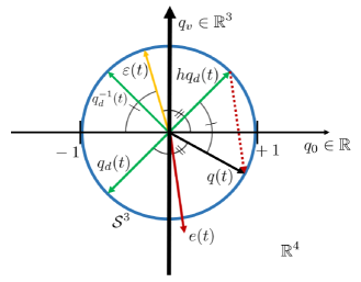
Figure 1: Illustration of the attitude tracking errors: The controller renders the tracking error $e(t)=q(t)-hq_{d}(t)\to 0_{4\times 1}$ in the space $\mathbb{R}^{4}$, which implies the quaternion error $\varepsilon(t)\to[h\ 0\ 0\ 0]^{T}$ in the unit sphere $\mathcal{S}^{3}$. Given the the initial conditions of $q$ and $q_{d}$ indicated in the figure, the shortest path, indicated by the single strip angles, to reach the same physical rotation is between $q$ and the reassigned desired trajectory with the initial condition $hq_{d}$ with $h=-1$. This implies the quaternion error $\varepsilon$ is driven to $[-1\ 0\ 0\ 0]^{T}$ in the closed loop.

The control objective is then to design a control law for $\bar{\tau}$ to render the attitude tracking error $e\to 0_{4\times 1}$ and $\dot{e}\to 0_{4\times 1}$ globally exponentially stable. This in turns implies that $q\to hq_{d}$ and $\dot{q}\to h\dot{q}_{d}$ globally exponentially. By $h\dot{q}_{d}=\frac{1}{2}J(hq_{d})\omega_{d}$ and Property 4 of the matrix $J(\cdot)$, it has $h^{2}\omega_{d}=2J^{T}(hq_{d})h\dot{q}_{d}$. In consequence, $q\to hq_{d}$ and $\dot{q}\to h\dot{q}_{d}$ implies $\omega\to h^{2}\omega_{d}=\omega_{d}$. Thus, with a little notation abuse, the desired trajectory $q_{d}$, $\dot{q}_{d}$ and $\ddot{q}_{d}$ will be used in the ideal state-feedback control design instead of the reassigned ones $hq_{d}$, $h\dot{q}_{d}$ and $h\ddot{q}_{d}$.

4.2 State-feedback Controller Design

Given the desired trajectory $q_{d},\dot{q}_{d}$, define the reference velocity as

$$\dot{q}_{r}=\dot{q}_{d}-\Lambda\left(q-q_{d}\right)$$ (35)

where $0<\Lambda=\Lambda^{T}\in\mathbb{R}^{4\times 4}$ is a gain matrix. Define the combined tracking error as

$$s=\dot{q}-\dot{q}_{r}=\dot{q}-\dot{q}_{d}+\Lambda\left(q-q_{d}\right).$$ (36)

The state-feedback tracking controller is readily proposed as

$$\bar{\tau}=D(q)\ddot{q}_{r}+C(q,\dot{q})\dot{q}_{r}-K_{s}s,$$ (37)

where $0<K_{s}=K_{s}^{T}\in\mathbb{R}^{4\times 4}$ together with matrix $\Lambda$ provides the PD-control action through $K_{s}s=K_{s}\dot{e}+K_{p}e$, with $K_{p}:=K_{s}\Lambda$. The actual control torque applied to the spacecraft is calculated by (13).

Theorem 5.

(Ideal State-feedback controller): The control law (37) in closed loop with the system (10) drives $q\to q_{d}$ and $\dot{q}\to\dot{q}_{d}$ exponentially from any initial conditions $q(0)\in\mathcal{S}^{3}$ and $\dot{q}(0)\in\mathbb{R}^{4}$.

Taking the time derivative of (36), premultiplying this by the matrix $D(q)$ in (9) and by the Lagrangian dynamics (10), gives

$$D(q)\dot{s} = D(q)(\ddot{q}-\ddot{q}_{r})$$

$$= -C(q,\dot{q})\dot{q}+\bar{\tau}-D(q)\ddot{q}_{r}.$$

This error dynamics in closed loop with the controller (37) results in

$$D(q)\dot{s} = -C(q,\dot{q})\dot{q}+C(q,\dot{q})\dot{q}_{r}-K_{s}s,$$ (38)

$$= -C(q,\dot{q})s-K_{s}s.$$

On the other hand, by (36) the attitude error dynamics (32) is rewritten as

$$\dot{e}=\dot{q}-\dot{q}_{d}=s-\Lambda e.$$ (39)

Notice that the error dynamics (38)-(39) has the origin $s=0_{4\times 1}$, $e=0_{4\times 1}$ as the unique equilibrium. Consider the Lyapunov function candidate

$$V_{1}=\frac{1}{2}s^{T}D(q)s+\frac{\alpha}{2}e^{T}e$$ (40)

for some $\alpha>0$ that verifies $\alpha I_{4}<4K_{s}\Lambda=4K_{p}$. Clearly, this Lyapunov function candidate is radially unbounded. The time derivative of (40) is

$$\dot{V}_{1}=s^{T}D(q)\dot{s}+\frac{1}{2}s^{T}\dot{D}(q)s+\alpha e^{T}\dot{e}.$$

Its time evolution along the error dynamics (38)-(39) is

$$\dot{V}_{1} =s^{T}\left(-C(q,\dot{q})s-K_{s}s\right)+\frac{1}{2}s^{T}\dot{D}(q)s+\alpha e^{T}\left(s-\Lambda e\right)$$

$$=-s^{T}K_{s}s+\alpha e^{T}s-\alpha e^{T}\Lambda e$$

$$=-\left[\begin{array}[]{cc}s^{T}&e^{T}\end{array}\right]\left[\begin{array}[]{cc}K_{s}&-\frac{\alpha}{2}I_{4}\\ -\frac{\alpha}{2}I_{4}&\alpha\Lambda\end{array}\right]\left[\begin{array}[]{c}s\\ e\end{array}\right]$$ (46)

where the skew symmetry (15) of the matrix $\dot{D}(q)-2C(q,\dot{q})$ in Lemma 2 is used. Thus, (4.2) is negative definite, concluding that the equilibrium $s=0_{4\times 1}$, $e=0_{4\times 1}$ is uniformly globally exponentially stable. This implies that $q(t)\to q_{d}(t)$ and $\dot{q}(t)\to\dot{q}_{d}(t)$ exponentially from any initial conditions $q(0)\in\mathcal{S}^{3}$, $\dot{q}(0)\in\mathbb{R}^{4}$.

$\square$

Remark 6.

(State-feedback controller): The control law (37) has been widely studied for tracking control designs for mechanical systems in Euclidean space, particularly for robot manipulators. The proposed 4-DOF Lagrangian approach allows to bridge up the gap between control designs for mechanical systems in Euclidean space and control designs for the attitude of a rigid body in the quaternion group, and to enable using the whole quaternion in attitude control designs, in contrast to control designs that use only the vector part of the quaternion [47, 52], avoiding the topological obstruction discussed in [35, 36] and singularities in controller development using any 3-DOF Lagrangian dynamics to describe the attitude of a rigid body [51, 50, 49, 47, 21]. The global exponential convergence of the tracking error by the continuous controller (37) is achieved on the Euclidean space $\mathbb{R}^{4}$ by designing the control law that renders the origin $(e,\ \dot{e})=0$ globally exponentially stable. Notice that $q(t),\ q_{d}(t)\in\mathcal{S}^{3}$ for all $t\geq 0$, so does the quaternion error $\varepsilon(t)$ defined in (33). The convergence to the origin of $e(t)$ implies the convergence of the quaternion error $\varepsilon(t)$ to the quaternion identity in the quaternion group $\mathcal{S}^{3}$.

Compared to the results based on Euler-Newtonian dynamics [26, 27, 48, 30, 64, 42, 33], the proposed controller achieves the global exponential stability without the need of addressing the singularity issues.

4.3 Hybrid State-feedback Controller

When the quaternion measurements are clean, the initial assignment of the desired quaternion in (34) ensures the tracking error $e(t)$ to converge to the origin under the control law (37) and (13). The convergence to the origin of the tracking error $e(t)$ implies convergence of the quaternion error $\epsilon(t)$ in (31) to either of the two disconnected antipodal points on $S^{3}$. Without a careful treatment of the ambiguity, however, it may become sensitive to small quaternion measurement noise [36]. To deal with this issue, motivated by the recent works [39, 41] this subsection presents a hybrid state-feedback controller. The main idea is to make the switching as in (32) each time when a switch condition is satisfied, depending on a potential function $\mathcal{U}(e)$ measuring the closeness to one of these two antipodal points.

Let $\mathcal{H}=\{-1,1\}\subset\mathbb{N}$ be an index set, and $\mathcal{U}\vcentcolon\mathbb{R}^{4}\times\mathcal{H}\to\mathbb{R}_{+}$ be a potential function with respect to the set $\mathcal{A}_{0}=\{0_{4\times 1}\}\times\mathcal{H}$. That is, for each $h\in\mathcal{H}$, the map $e\mapsto\mathcal{U}(e,h)$ is continuously differentiable in $\mathcal{D}\subseteq\mathbb{R}^{4}\times\mathcal{H}$. In addition, $\mathcal{U}(e,h)$ verifies $\mathcal{U}(e,h)>0$ for all $(e,h)\notin\mathcal{A}_{0}$, $\mathcal{U}(e,h)=0$ for all $(e,h)\in\mathcal{A}_{0}$, and

$$\mathcal{G}(e)\vcentcolon=\mathcal{U}(e,h)-\underset{m\in\mathcal{H}}{\min}\;\mathcal{U}(e,m)>\delta,$$ (47)

for some $\delta>0$. Then, inspired by the switching mechanism of [42] the discrete state $h$, which dictates the current mode of the hybrid control system, is defined as

$$\left\{\begin{array}[]{cc}\dot{h}=0,&\;\;\mathrm{if}\ \mathcal{G}(e)\leq\delta,\\ h^{+}\in\arg\underset{m\in\mathcal{H}}{\min}\;\mathcal{U}(e,m),&\;\;\mathrm{if}\ \mathcal{G}(e)\geq\delta.\end{array}\right.$$ (48)

For the design of the hybrid controller, the potential function $\mathcal{U}(e,h)\vcentcolon=\|e\|^{2}$ is considered. Observe that its gradient with respect to $e$ is $\nabla\mathcal{U}=2e$, which vanishes only at $\mathcal{A}_{0}$.

Let the set of critical points for $\mathcal{U}(e,h)$ be defined as $\Omega_{0}=\{(e,h)\;|\;e=0_{4\times 1}\}$ for $(e,h)\in\mathcal{D}$. Note that all potential functions $e\mapsto\mathcal{U}(e,h)$, $\forall h\in\mathcal{H}$, share the same critical point $e=0_{4\times 1}$, i.e., the potential function $\mathcal{U}$ is centrally synergistic with a gap exceeding $\delta>0$ [39, 38].

The proposed hybrid controller consists of (13),

$$\bar{\tau} =D(q)\ddot{q}_{r}+C(q,\dot{q})\dot{q}_{r}-K_{s}s(\dot{e},e,h),$$ (49)

$$\dot{q}_{r} =\dot{q}_{d}-\Lambda e,$$ (50)

$$s =\dot{e}+\Lambda e,$$ (51)

$$e =q-hq_{d},$$ (52)

$$\dot{e} =\dot{q}-h\dot{q}_{d},$$ (53)

and the switching mechanism (48).

Theorem 7.

(Hybrid state-feedback controller): The hybrid controller (13), (49)-(53), and (48) in closed loop with the system (10) stabilizes the set $\mathcal{A}_{1}:=\{(e,s,h)\in\mathcal{X}_{1}|e=0_{4\times 1},s=0_{4\times 1}\}$ globally exponentially, where $\mathcal{X}_{1}\vcentcolon=\mathbb{R}^{4}\times\mathbb{R}^{4}\times\mathcal{H}$.

Define $\zeta_{1}\vcentcolon=\left(e,s,h\right)\in\mathcal{X}_{1}$. Then, the closed-loop system is described by

$$\left.\begin{array}[]{rl}\dot{e}=&s-\Lambda e\\ D(q)\dot{s}=&-C(q,\dot{q})s-K_{s}s\\ \dot{h}=&0\end{array}\right\}\quad\forall\zeta_{1}\in\bar{C}_{1},$$ (54)

$$\zeta_{1}^{+}=\left[\begin{array}[]{c}e\\ s\\ h^{+}\end{array}\right],\quad\forall\zeta\in\bar{D}_{1},$$ (55)

where $\zeta_{1}^{+}$ is the state value right after the jump, $h^{+}$ is given in (48), and $\bar{C}_{1}$ and $\bar{D}_{1}$ represent the flow set and the jump set, respectively, given by

$$\bar{C}_{1} =\{\zeta_{1}\in\mathcal{X}_{1}\ |\ \mathcal{G}(e)\leq\delta\},$$ (56)

$$\bar{D}_{1} =\{\zeta_{1}\in\mathcal{X}_{1}\;|\;\mathcal{G}(e)\geq\delta\}.$$ (57)

Consider the following Lyapunov function candidate

$$V_{2}(\zeta_{1})=\frac{1}{2}s^{T}D(q)s+\frac{\alpha}{2}\mathcal{U}(e,h),$$ (58)

for some $0<\alpha<4\lambda_{\min}(K_{s})\lambda_{\min}(\Lambda)$. Note that $V_{2}$ is bounded by $\frac{1}{2}z^{T}M_{1}z\leq V_{2}\leq\frac{1}{2}z^{T}M_{2}z$, with $z=\left[\|s\|,\|e\|\right]^{T}$, and

$$M_{1}=\left[\begin{array}[]{cc}\underline{m}&0\\ 0&\frac{\alpha}{2}\end{array}\right],\quad M_{2}=\left[\begin{array}[]{cc}\bar{m}&0\\ 0&2\alpha\end{array}\right].$$

Then, in view of (4.2) and (48) the time derivative of $V_{2}$ along (54) for all $\zeta_{1}\in\bar{C}_{1}$ is given by

$$\dot{V}_{2} =-s^{T}K_{s}s+\alpha e^{T}s-\alpha e^{T}\Lambda e,$$

$$\leq-z^{T}\left[\begin{array}[]{cc}\lambda_{\min}(K_{s})&-\frac{\alpha}{2}\\ -\frac{\alpha}{2}&\alpha\lambda_{\min}(\Lambda)\end{array}\right]z$$ (61)

$$=-z^{T}M_{3}z\leq-\lambda_{c}V_{2},$$ (62)

where $\lambda_{c}\vcentcolon=\frac{\lambda_{\min}(M_{3})}{\lambda_{\max}(M_{2})}>0$. Therefore, the states $s,e\in\mathbb{R}^{4}$ are bounded for any $h\in\mathcal{H}$, and $\zeta_{1}\in\bar{C}_{1}$.

In the jump set $\zeta_{1}\in\bar{D}_{1}$, it yields

$$V_{2}(\zeta_{1}^{+})-V_{2}(\zeta_{1}) =\frac{1}{2}s^{T}D(q)s+\frac{\alpha}{2}\mathcal{U}(e,h^{+})$$

$$\quad-\frac{1}{2}s^{T}D(q)s-\frac{\alpha}{2}\mathcal{U}(e,h)$$

$$\leq-\frac{\alpha}{2}\delta,$$ (63)

therefore, for $\alpha>1$, $V_{2}$ is strictly decreasing over the jump set $\bar{D}_{1}$. Thus, $\zeta_{1}(t)$ is bounded for all $t\geq 0$. Similar to the proof of Theorem 2 in [39], it follows that $V_{2}(\zeta_{1}(t,j))\leq\mathrm{e}^{-\lambda_{2}(t+j)}V_{2}(\zeta_{1}(0,0))$ for all $(t,j)\in\mathrm{dom}\zeta_{1}$, where $\lambda_{2}=\min\left\{\lambda_{c},-\ln{\left(1-\frac{\alpha\delta}{4\bar{v}}\right)}\right\}$, given $V_{2}\leq\bar{v}$. Therefore, the equilibrium point $(s,e)=(0_{4\times 1},0_{4\times 1})$ is globally exponentially stable.

$\square$

Remark 8.

(The centrally synergistic potential function $\mathcal{U}(e,h)$): The potential function $\mathcal{U}(e,h)=\|e\|^{2}$, for $e=q-hq_{d}$ can be expressed in terms of the scalar part $\varepsilon_{0}$ of the quaternion error $\varepsilon$ (33) as $\mathcal{U}(e(\varepsilon_{0}),h)=2(1-h\varepsilon_{0}):=\mathcal{U}_{\varepsilon}(\varepsilon_{0},h)$ (shown in Fig. 2). This potential function has been widely used to globally stabilize the set $\mathcal{A}=\{\pm\hat{1}\}\times\mathcal{H}$, where $\hat{1}=[1,0,0,0]^{T}\in\mathcal{S}^{3}$, see for instance [43, 36, 40]. However, the potential function $\mathcal{U}_{\varepsilon}(\varepsilon_{0},h)$ relative to $\mathcal{A}$ is not central , i.e., the potential functions $\varepsilon\mapsto\mathcal{U}_{\varepsilon}(\varepsilon_{0},h)$, for $h\in\mathcal{H}$, have different critical points $\pm\hat{1}$. On the other hand, the potential function $\mathcal{U}(e,h)=\|e\|^{2}$ relative to $\mathcal{A}_{0}$ is central, for having the same critical point $e=0_{4\times 1}$ for $h\in\mathcal{H}$, which guarantees that each mode of the hybrid closed-loop system is almost globally exponentially stable [39].

Notice that unlike the potential function defined in a manifold, e.g., $SO(3)$ or $\mathcal{S}^{3}$ [39, 41], the potential function $\mathcal{U}_{\varepsilon}(\varepsilon_{0},h)$ has a unique feature of containing no undesired critical points since both $\varepsilon_{0}=\pm 1$ achieve the attitude tracking $R=R_{d}$. On the other hand, since the controller design is carried out on $\mathbb{R}^{4}$, the potential function $\mathcal{U}(e,h)$ has only one critical point, which corresponds to the desired equilibrium.

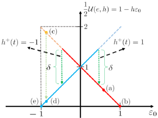
Figure 2: Illustration of the potential function. The potential function $\mathcal{U}(e,h)$ is represented by the red and blue solid lines corresponding to $\mathcal{U}(e,1)$ and $\mathcal{U}(e,-1)$, respectively. They are extended by the dashed lines corresponding to the switching zone, i.e., where $\mathcal{U}(e,h)-\underset{m\in\mathcal{H}}{\min}\;\mathcal{U}(e,m)\geq\delta$. Any trajectory starting in the red solid line under the continuous controller of Theorem 5, for example (a), is led to $1$ (b). On the other hand, any point in the blue solid line (d) is led to $-1$ (e). Notice that under a noisy condition a trajectory starting at (a), which would converge to (b) in the noise-free condition, can be led to (c) under a ”larger” noise level, where $\mathcal{U}(e,1)-\mathcal{U}(e,-1)\geq\delta$. Given that $\underset{m\in\mathcal{H}}{\min}\;\mathcal{U}(e,m)=\mathcal{U}(e,-1)$ in (c), the hybrid controller in Corollary 7 performs a jump $h^{+}=1$, to (d). Consequently, this trajectory eventually converges to (e).

4.4 Adaptive Hybrid State-feedback Controller

This subsection addresses the issue of parameter uncertainty of the inertia matrix $\theta\in\mathbb{R}^{6}$ in (19) and on-orbit disturbance torque, assumed to be an unknown constant vector. This assumption is made for simplicity and it is a good model for on-orbit torque disturbances as justified in [42]. Furthermore, the adaptive control law given in this subsection can track slowly time-varying torque disturbances.

The Lagrangian system (10) in the presence of disturbances $p\in\mathbb{R}^{3}$ can be expressed as

$$D(q)\ddot{q}+C(q,\dot{q})\dot{q}=\bar{\tau}+d,$$ (64)

where $d\in\mathbb{R}^{4}$ is

$$d=\frac{1}{2}J(q)p=\frac{1}{2}Q(q)\bar{p},$$ (65)

with $\bar{p}\vcentcolon=\left[0,\ p^{T}\right]^{T}\in\mathbb{R}^{4}$ representing the unknown constant disturbance. By the linear parameterization (16) in Lemma 3, the dynamics (64) can be rewritten as

$$Y_{0}(q,\dot{q},\ddot{q})m_{0}+\bar{Y}(q,\dot{q},\ddot{q})\Theta =\bar{\tau},$$ (66)

where $\Theta\vcentcolon=\left[\theta^{T},\ p^{T}\right]^{T}\in\mathbb{R}^{9}$ is the augmented vector of unknown parameters. The regressor $\bar{Y}(q,\dot{q},\ddot{q})\in\mathbb{R}^{4\times 9}$ is defined as

$$\bar{Y}(q,\dot{q},\ddot{q})=\left[Y(q,\dot{q},\ddot{q})\ -\frac{1}{2}J(q)\right].$$ (67)

Define the parameter error

$$\tilde{\Theta}=\hat{\Theta}-\Theta,$$ (68)

with $\hat{\Theta}\in\mathbb{R}^{9}$ the parameter estimate, and an auxiliary variable $\eta_{1}\in\mathbb{R}^{4}$

$$\eta_{1}=\dot{e}+e,$$ (69)

with $\dot{e},e\in\mathbb{R}^{4}$ given by (52) and (53), respectively.

Let the state be $\zeta_{2}=\left(e,\eta_{1},\tilde{\Theta},h\right)\in\mathcal{X}_{2}\vcentcolon=\mathbb{R}^{4}\times\mathbb{R}^{4}\times\mathbb{R}^{9}\times\mathcal{H}$, where the discrete state $h\in\mathcal{H}$ defined in (48). Then, the flow set and the jump set are given by

$$\bar{C}_{2} =\{\zeta_{2}\in\mathcal{X}_{2}\ |\ \mathcal{G}(e)\leq\delta\},$$ (70)

$$\bar{D}_{2} =\{\zeta_{2}\in\mathcal{X}_{2}\;|\;\mathcal{G}(e)\geq\delta\}.$$ (71)

The following adaptive state-feedback controller is proposed

$$\bar{\tau}=Y_{d_{0}}m_{0}+\bar{Y}_{d}\hat{\Theta}-K_{d}\eta_{1}-k_{p}e,$$ (72)

where $0<K_{d}^{T}=K_{d}\in\mathbb{R}^{4\times 4}$ and, $k_{p}>0$ are design parameters. The feedforward compensation is given by $Y_{d_{0}}m_{0}+\bar{Y}_{d}\hat{\Theta}=D(q_{d})\ddot{q}_{d}+C(q_{d},\dot{q}_{d})\dot{q}_{d}$, with $Y_{d_{0}}\vcentcolon=Y_{0}(q_{d},\dot{q}_{d},\ddot{q}_{d})$ and $\bar{Y}_{d}\vcentcolon=\bar{Y}(q_{d},\dot{q}_{d},\ddot{q}_{d})$ given in (17) and (67), respectively.

The parameter estimate $\hat{\Theta}$ is updated according to the following adaptation law

$$\dot{\hat{\Theta}} =-\gamma_{1}Y^{T}_{f}\left(\hat{\tau}_{f}-\tau_{f}\right)-\gamma_{2}\bar{Y}^{T}_{d}\eta_{1},$$ (73)

$$\hat{\tau}_{f} =Y_{f}\hat{\Theta},$$ (74)

with $\gamma_{1}>0$, $\gamma_{2}>0$ design parameters. Additionally, matrix $Y_{f}(q,\dot{q},q_{f})\in\mathbb{R}^{4\times 9}$, and vectors $\tau_{f}\in\mathbb{R}^{4}$, $q_{f}\in\mathbb{R}^{4}$ are obtained by a first-order linear filter, aimed at avoiding $\ddot{q}$ to appear in the regressors, as follows

$$Y_{f}(q,\dot{q},q_{f}) =\left[\lambda_{f}J(q)F(w)-X_{f}\;\;-\frac{1}{2}J(q_{f})\right],$$ (75)

$$\dot{X}_{f} =\lambda_{f}\left(X-X_{f}\right),\quad X_{f}(0)=X(0),$$ (76)

$$X \vcentcolon=\lambda_{f}J(q)F(w)-2J(q)S(w)F(w)$$

$$\quad+J(\dot{q})F(w),$$ (77)

$$\dot{\tau}_{f} =\lambda_{f}\left(\bar{\tau}-\tau_{f}\right),\quad\tau_{f}(0)=\bar{\tau}(0),$$ (78)

$$\dot{q}_{f} =\lambda_{f}\left(q-q_{f}\right),\quad q_{f}(0)=q(0),$$ (79)

with $\lambda_{f}>0$ the filter gain. Map $F(\cdot)$ and vector $w\vcentcolon=J^{T}(q)\dot{q}\in\mathbb{R}^{3}$ are given in Lemma 3.

Theorem 9.

(Adaptive hybrid state-feedback controller): Choose the design parameters $k_{p}>0$, $\gamma_{1}>0$, $\gamma_{2}>0$, $\lambda_{f}>0$, $m_{0}>0$, and matrix $K_{d}=K^{T}_{d}>0$ such that

$$\lambda_{\min}\left(K_{d}\right) >\frac{(\alpha_{1}+\alpha_{2})^{2}}{4k_{p}}+\alpha_{1},$$ (80)

where

$$\alpha_{1} =k_{h_{1}}+2k_{c_{1}}+\bar{m},$$ (81)

$$\alpha_{2} =k_{h_{2}}+k_{c_{1}}\|\dot{q}_{d}\|.$$ (82)

Then, the hybrid adaptive state-feedback control law (72) and (73)-(79) in closed loop with the system (64) stabilizes the set $\mathcal{A}_{2}\vcentcolon=\{(e,\eta_{1},h)\in\mathbb{R}^{4}\times\mathbb{R}^{4}\times\mathcal{H}|e=0_{4\times 1},\eta_{1}=0_{4\times 1}\}$ globally asymptotically, while $\tilde{\Theta}$ is maintained bounded.

Notice that dynamics (64) can be expressed, in view of Property 2 in Lemma 3, as

$$\frac{d}{dt}\left(D(q)\dot{q}\right)-C(q,\dot{q})^{T}\dot{q}-d=\bar{\tau}.$$ (83)

Therefore, by (83) and (75) the filtered torque $\tau_{f}$ obtained from (78) is expressed as

$$\tau_{f}=Y_{f}\Theta.$$ (84)

Taking the time derivative of the parameter error (68) and substituting (73) and (84), yields

$$\dot{\tilde{\Theta}}=-\gamma_{1}Y^{T}_{f}Y_{f}\tilde{\Theta}-\gamma_{2}\bar{Y}^{T}_{d}\eta_{1}.$$ (85)

The dynamics of $\eta_{1}$ is obtained by premultiplying the inertia matrix $D(q)$ with the time derivative of (69) as

$$D(q)\dot{\eta}_{1} =D(q)\ddot{q}-D(q)\ddot{q}_{d}+D(q)\dot{e},$$

$$=-C(q,\dot{q})\dot{q}+\bar{\tau}+d-D(q)\ddot{q}_{d}+D(q)\dot{e},$$

where (64) is used. Substituting the controller (72) into this last equation and after some arrangement yields

$$D(q)\dot{\eta}_{1} =-C(q,\dot{q})\eta_{1}-K_{d}\eta_{1}-k_{p}e+\bar{Y}_{d}\tilde{\Theta}+\chi_{1},$$ (86)

where $\chi_{1}\in\mathbb{R}^{4}$ is defined as

$$\chi_{1}=\underline{h}(t,e,\dot{e})+C(q,\dot{q})e+D(q)\dot{e},$$ (87)

with $\underline{h}(t,e,\dot{e})$ the residual dynamics defined in (7). By Property 7 in Lemma 3, $\chi_{1}$ can be upper bounded by

$$\|\chi_{1}\|\leq\alpha_{1}\|\eta_{1}\|+(\alpha_{1}+\alpha_{2})\|e\|,$$ (88)

with $\alpha_{1}$ and $\alpha_{2}$ given in (81)-(82).

Therefore, the closed-loop system is given by

$$\underbrace{\begin{array}[]{rl}\dot{e}=&-e+\eta_{1}\\ D(q)\dot{\eta}_{1}=&-C(q,\dot{q})\eta_{1}-K_{d}\eta_{1}-k_{p}e+\bar{Y}_{d}\tilde{\Theta}+\chi_{1}\\ \dot{\tilde{\Theta}}=&-\gamma_{1}Y^{T}_{f}Y_{f}\tilde{\Theta}-\gamma_{2}\bar{Y}^{T}_{d}\eta_{1}\\ \dot{h}=&0\end{array}}_{\forall\zeta_{2}\in\bar{C}_{2}}$$ (89)

$$\zeta^{+}_{2}=\left[\begin{array}[]{c}e\\ \eta_{1}\\ \tilde{\Theta}\\ h^{+}\end{array}\right],\quad\forall\zeta_{2}\in\bar{D}_{2}.$$ (90)

Let $V_{3}(\zeta_{2})$ be a Lyapunov function candidate defined as

$$V_{3}(\zeta_{2})=\frac{1}{2}\eta^{T}_{1}D(q)\eta_{1}+\frac{k_{p}}{2}\mathcal{U}(e,h)+\frac{1}{2\gamma_{2}}\tilde{\Theta}^{T}\tilde{\Theta}.$$ (91)

Then, $V_{3}$ is bounded by $\frac{1}{2}z^{T}M_{3}z\leq V_{3}\leq\frac{1}{2}z^{T}M_{4}z$, where $z=\left[\|\eta_{1}\|,\|e\|,\|\tilde{\Theta}\|\right]$ and

$$M_{3}=\left[\begin{array}[]{ccc}\underline{m}&0&0\\ 0&\frac{k_{p}}{2}&0\\ 0&0&\frac{1}{2\gamma_{2}}\end{array}\right],\quad M_{4}=\left[\begin{array}[]{ccc}\bar{m}&0&0\\ 0&k_{p}&0\\ 0&0&\frac{1}{\gamma_{2}}\end{array}\right].$$

The time derivative of (91) along (89) for all $\zeta_{2}\in\bar{C}_{2}$ is

$$\dot{V}_{3} =\eta^{T}_{1}D(q)\dot{\eta}_{1}+\frac{1}{2}\eta^{T}_{1}\dot{D}(q)\eta_{1}+k_{p}e^{T}\dot{e}+\frac{1}{\gamma_{2}}\tilde{\Theta}^{T}\dot{\tilde{\Theta}}$$

$$=\eta^{T}_{1}\left(-C(q,\dot{q})\eta_{1}-K_{d}\eta_{1}-k_{p}e+\bar{Y}_{d}\tilde{\Theta}+\chi_{1}\right)$$

$$\quad+\frac{1}{2}\eta^{T}_{1}\dot{D}(q)\eta_{1}+k_{p}e^{T}\left(-e+\eta_{1}\right)$$

$$\quad+\frac{1}{\gamma_{2}}\tilde{\Theta}^{T}\left(-\gamma_{1}Y^{T}_{f}Y_{f}\tilde{\Theta}-\gamma_{2}\bar{Y}^{T}_{d}\eta_{1}\right)$$

$$=-\eta^{T}_{1}K_{d}\eta_{1}-k_{p}e^{T}e+\eta^{T}_{1}\chi_{1}-\frac{\gamma_{1}}{\gamma_{2}}\tilde{\Theta}^{T}Y^{T}_{f}Y_{f}\tilde{\Theta}$$

$$\leq-\lambda_{\min}(K_{d})\|\eta_{1}\|^{2}-k_{p}\|e\|^{2}+\alpha_{1}\|\eta_{1}\|^{2}$$

$$\quad+(\alpha_{1}+\alpha_{2})\|\eta_{1}\|\|e\|-\frac{\gamma_{1}}{\gamma_{2}}\lambda_{\min}\left(Y^{T}_{f}Y_{f}\right)\|\tilde{\Theta}\|^{2}$$

$$=-z^{T}\Phi_{1}z,$$ (92)

where (88) and the skew-symmetric property (15) of Lemma 2 are used. The matrix $\Phi_{1}\in\mathbb{R}^{3\times 3}$ in (4.4) is given by

$$\Phi_{1}=\left[\begin{array}[]{ccc}\lambda_{\min}(K_{d})-\alpha_{1}&-\frac{(\alpha_{1}+\alpha_{2})}{2}&0\\ -\frac{(\alpha_{1}+\alpha_{2})}{2}&k_{p}&0\\ 0&0&\frac{\gamma_{1}}{\gamma_{2}}\lambda_{\min}\left(Y^{T}_{f}Y_{f}\right)\end{array}\right],$$ (93)

which is, under condition (80), semi-negative definite. Therefore, state $\eta_{1},e\in\mathbb{R}^{4}$ and $\tilde{\Theta}\in\mathbb{R}^{9}$ remain bounded for all $\zeta_{2}\in\bar{C}_{2}$. On the other hand, noticing that neither $\eta_{2}$ nor $\tilde{\Theta}$ change over the jumps, it has for $\zeta_{2}\in\bar{D}_{2}$ that

$$V_{3}(\zeta^{+}_{2})-V_{3}(\zeta_{2}) =\frac{k_{p}}{2}\mathcal{U}(e,h^{+})-\frac{k_{p}}{2}\mathcal{U}(e,h)$$

$$\leq-\frac{k_{p}}{2}\delta.$$ (94)

Thus, $V_{3}(\zeta_{2})$ is non-increasing under condition (80) along trajectories of the closed-loop system for all $\zeta_{2}\in\bar{C}_{2}$, and strictly decreasing over the jump set $\bar{D}_{2}$ provided that $k_{p}>0$. Therefore, the set $\mathcal{A}_{2}$ is uniformly globally stable.

Denote $t_{j}>0$ the time of the $j$th jump for some $j\in\mathbb{N}$. Then, in view of (4.4) and using the same arguments as in the proof of Theorem 3.1 in [65], it can be expressed $V_{3}(\zeta^{+}_{2}(t_{j}))-V_{3}(\zeta_{2}(0))<-j\sigma$, with $\sigma\vcentcolon=\frac{k_{p}}{2}\delta>0$. Therefore, for any $V_{3}(\zeta_{2}(t_{j}))>0$ it yields $j<V_{3}(\zeta_{2}(0))/\sigma$, which implies that the number of jumps is finite. Then, assuming $\zeta_{2}\in\bar{C}_{2}$, and relying on the fact that the states $\eta_{1},e\in\mathbb{R}^{4}$ and $\tilde{\Theta}\in\mathbb{R}^{9}$ are bounded, it is straightforward to verify that $\ddot{V}_{3}$ is bounded. Thus, by invoking the Barbalat’s Lemma, it concludes that $\dot{V}_{3}\to 0$ as $t\to\infty$. In consequence, the set $\mathcal{A}_{2}$ is uniformly globally asymptotically stable.

$\square$

Remark 10.

The adaptation law (73)-(74) in its analysis form (85) coincides with the so-called composite adaptation law used for robot control (Eq. (8.125), [2]). It has a smother and faster convergence behavior due to its first-order dynamics in (85). If, in addition, the following persistent excitation

$$\int^{t+T}_{t}Y^{T}_{f}(\uptau)Y_{f}(\uptau)d\uptau\geq\lambda_{z}I_{9},\quad\forall t\geq 0$$ (95)

is fulfilled for the matrix $Y_{f}(t):=Y_{f}(q(t),\dot{q}(t),q_{f}(t))\in\mathbb{R}^{4\times 9}$ defined in (75) for some $T>0$ and $\lambda_{z}>0$, then it can be shown using the standard arguments of adaptive control for a linearly parametrized uncertainty (e.g., [2]) that the set $\{\zeta_{2}\in\mathcal{X}_{2}|e=0_{4\times 1},\eta_{1}=0_{4\times 1},\tilde{\Theta}=0_{9\times 1}\}$ is globally exponentially stable.

4.5 Adaptive Hybrid Attitude-feedback Controller

In this subsection, the issues of uncertainty in the inertial matrix, constant torque disturbances, and lack of angular-velocity measurements for feedback due to, for instance, gyros sensor failures, and unknown inertia matrix are addressed. The damping term required in the control action is provided by a nonlinear filter, similar to that proposed in [48].

Let the auxiliary variable $\eta_{2}$ be defined as

$$\eta_{2}=\dot{e}+e+\nu$$ (96)

where $e$ and $\dot{e}$ are defined in (52) and (53), respectively. The required damping is achieved through the nonlinear filter

$$\dot{e}_{f} =-\mathrm{Cosh}^{2}(e_{f})\left(K_{f}\nu+k_{v}\eta_{2}-k_{p}e\right),$$ (97)

$$\nu =\mathrm{Tanh}(e_{f}),$$ (98)

with the initial condition $e_{f}(0)=0_{4\times 1}$, where the hyperbolic functions are entry-wise defined vectors and matrix, respectively

$$\mathrm{Tanh}(e_{f}) :=[\tanh{(e_{f_{1}})},...,\tanh{(e_{f_{4}})}]^{T}\in\mathbb{R}^{4}$$

$$\mathrm{Cosh}(e_{f}) :=\mathrm{diag}\{\cosh{(e_{f_{1}})},\ldots,\cosh{(e_{f_{4}})}\}\in\mathbb{R}^{4\times 4},$$

the gain $K_{f}\in\mathbb{R}^{4\times 4}$ is a positive definite symmetric matrix and, $k_{p}>0$ and $k_{v}>0$ are positive constants.

Note that, according to (98), it has

$$\|\nu\|=\|\mathrm{Tanh}(e_{f})\|\leq 2.$$ (99)

Implementation of the nonlinear filter (98) requires $\dot{e}$ involved in the auxiliary variable $\eta_{2}$, which can be eliminated in a similar way to that of [66]:

$$\dot{g} =-K_{f}\left(g-k_{v}e\right)-k_{v}\left(g+(1-k_{v})e\right)+k_{p}e$$ (100)

$$\nu =g-k_{v}e$$ (101)

with the initial condition $g(0)=k_{v}e(0)$.

Consider the perturbed system (66)-(67), with torque disturbance $p\in\mathbb{R}^{3}$, and the augmented vector of unknown parameters $\Theta=\left[\theta^{T},p^{T}\right]^{T}$. Then, the adaptive attitude-feedback controller is proposed as

$$\bar{\tau}=Y_{d_{0}}m_{0}+\bar{Y}_{d}\hat{\Theta}+k_{v}\nu-k_{p}e,$$ (102)

where $Y_{d_{0}}\in\mathbb{R}^{4}$ and $\bar{Y}_{d}\in\mathbb{R}^{4\times 9}$ are defined in the same way as for controller (72). Likewise, let $\hat{\Theta}\in\mathbb{R}^{9}$ be the estimation of the augmented parameter vector, updated by the adaptive law

$$\hat{\Theta} =-\Gamma\bar{Y}^{T}_{d}e-\Gamma\mu$$ (103)

$$\dot{\mu} =\bar{Y}^{T}_{d}\left(e+\nu\right)-\dot{\bar{Y}}^{T}_{d}e$$ (104)

with $0<\Gamma=\Gamma^{T}\in\mathbb{R}^{9\times 9}$ being an adaptation gain matrix.

Let the state be defined as $\zeta_{3}=\left(e,\eta_{2},\nu,\tilde{\Theta},h\right)\in\mathcal{X}_{3}\vcentcolon=\mathbb{R}^{4}\times\mathbb{R}^{4}\times\mathbb{R}^{4}\times\mathbb{R}^{9}\times\mathcal{H}$, where the discrete state $h\in\mathcal{H}$ and the parameter error $\tilde{\Theta}$ are defined in (48) and (68), respectively. Then, the flow set and the jump set are given by

$$\bar{C}_{3} =\{\zeta_{3}\in\mathcal{X}_{3}\ |\ \mathcal{G}(e)\leq\delta\},$$ (105)

$$\bar{D}_{3} =\{\zeta_{3}\in\mathcal{X}_{3}\;|\;\mathcal{G}(e)\geq\delta\}.$$ (106)

Theorem 11.

(Adaptive hybrid attitude-feedback controller): Choose $K_{f}=K^{T}_{f}>0$, $\Gamma=\Gamma^{T}>0$, $k_{p}>0$ and

$$k_{v} >\frac{1}{\underline{m}}\left(\beta+\alpha_{1}\right),$$ (107)

where

$$\beta\vcentcolon =\max\left\{\frac{\alpha^{2}_{2}}{4k_{p}},\;\frac{\alpha^{2}_{3}k_{p}+\alpha^{2}_{2}\lambda_{\min}(K_{f})}{4k_{p}\lambda_{\min}(K_{f})}\right\}$$ (108)

$$\alpha_{1} =k_{h_{1}}+4k_{c_{1}}+\bar{m}$$ (109)

$$\alpha_{2} =k_{h_{1}}+k_{h_{2}}+k_{c_{1}}\|\dot{q}_{d}\|+4k_{c_{1}}+\bar{m}|k_{p}-1|$$ (110)

$$\alpha_{3} =k_{h_{1}}+k_{c_{1}}\|\dot{q}_{d}\|+4k_{c_{1}}+\bar{m}\|K_{f}+I_{4}\|$$ (111)

and $k_{c_{1}}$, $k_{c_{2}}$, $k_{h_{1}}$, $k_{h_{2}}$, $\underline{m}$ and $\bar{m}$ are defined in Lemma 2 and Lemma 3. Then, the control law (102) in closed loop with the system (64) renders the set $\mathcal{A}_{3}\vcentcolon=\{(e,\eta_{2},\nu,h)\in\mathbb{R}^{4}\times\mathbb{R}^{4}\times\mathbb{R}^{4}\times\mathcal{H}|e=0_{4\times 1},\eta_{2}=0_{4\times 1},\nu=0_{4\times 1}\}$ globally asymptotically stable, while maintaining the parameter estimation error $\tilde{\Theta}$ bounded.

For all $\zeta_{3}\in\bar{C}_{3}$, the time derivative of (98), by substituting $\dot{e}_{f}$, is given by

$$\dot{\nu} =\mathrm{Sech}^{2}(e_{f})\dot{e}_{f}=-K_{f}\nu-k_{v}\eta_{2}+k_{p}e$$ (112)

where $\mathrm{Sech}(x)\vcentcolon=\mathrm{diag}\{\mathrm{sech}(x_{1}),\ldots,\mathrm{sech}(x_{4})\}$ $\in$ $\mathbb{R}^{4\times 4}$ $\forall x\in\mathbb{R}^{4}$.

Taking the time derivative of (96) and premultiplying it by the inertial matrix $D(q)$ gives

$$D(q)\dot{\eta}_{2} =D(q)\left(\ddot{e}+\dot{e}+\dot{\nu}\right)$$

$$=D(q)\ddot{q}-D(q)\ddot{q}_{d}+D(q)\dot{e}+D(q)\dot{\nu},$$

where, with a little abuse of notation, $q_{d}$, $\dot{q}_{d}$, $\ddot{q}_{d}$ are considered instead of $hq_{d}$, $h\dot{q}_{d}$, $h\ddot{q}_{d}$ for $\zeta_{3}\in\bar{C}_{3}$.

Substituting the system (64) and the dynamics (112) gets

$$D(q)\dot{\eta}_{2} =-C(q,\dot{q})\dot{q}+\bar{\tau}+d-D(q)\ddot{q}_{d}+D(q)\dot{e}$$

$$\quad+D(q)\left(-K_{f}\nu-k_{v}\eta_{2}+k_{p}e\right),$$

which in closed loop with the control law (102) results in

$$D(q)\dot{\eta}_{2}=-C(q,\dot{q})\eta_{2}+k_{v}\nu-k_{p}e-k_{v}D(q)\eta_{2}+\bar{Y}_{d}\tilde{\Theta}+\chi_{2},$$ (113)

where

$$\chi_{2}=\underline{h}(t,e,\dot{e})+C(q,\dot{q})(e+\nu)+D(q)\left(\dot{e}-K_{f}\nu+k_{p}e\right)$$ (114)

with $\underline{h}(t,e,\dot{e})$ defined in (7).

By Lemma 3 and the upper bound (99), it can be shown that $\chi_{2}$ is bounded by

$$\|\chi_{2}\|\leq\alpha_{1}\|\eta_{2}\|+\alpha_{2}\|e\|+\alpha_{3}\|\nu\|,$$ (115)

where the constants $\alpha_{1}$, $\alpha_{2}$ and $\alpha_{3}$ are defined in (109)-(111).

Substituting the time derivative of the parameter estimate (103) in the time evolution of the parameter error $\tilde{\Theta}=\hat{\Theta}-\Theta$, gives

$$\dot{\tilde{\Theta}}=\dot{\hat{\Theta}}-\dot{\Theta}=-\Gamma\bar{Y}^{T}_{d}\eta_{2}.$$ (116)

Then the closed-loop system is given by

$$\underbrace{\begin{array}[]{cl}\dot{e}=&\eta_{2}-e-\nu,\\ D(q)\dot{\eta}_{2}=&-C(q,\dot{q})\eta_{2}+k_{v}\nu-k_{p}e-k_{v}D(q)\eta_{2}+\bar{Y}_{d}\tilde{\Theta}\\ &+\chi_{2},\\ \dot{\nu}=&-K_{f}\nu-k_{v}\eta_{2}+k_{p}e,\\ \dot{\tilde{\Theta}}=&-\Gamma\bar{Y}^{T}_{d}\eta_{2},\\ \dot{h}=&0,\end{array}}_{\forall\zeta_{3}\in\bar{C}_{3}}$$ (117)

$$\zeta^{+}_{3}=\left[\begin{array}[]{c}e\\ \eta_{2}\\ \nu\\ \tilde{\Theta}\\ h^{+}\end{array}\right],\quad\forall\zeta_{3}\in\bar{D}_{3}.$$ (118)

Notice that, in view of the definition (98), the state $\nu$ does not change over jumps.

Define the following Lyapunov function candidate

$$V_{4}=\frac{1}{2}\eta^{T}_{2}D(q)\eta_{2}+\frac{k_{p}}{2}\mathcal{U}(e,h)+\frac{1}{2}\nu^{T}\nu+\frac{1}{2}\tilde{\Theta}^{T}\Gamma^{-1}\tilde{\Theta},$$ (119)

which is radially unbounded. Its time evolution along the closed-loop system (117), for all $\zeta_{3}\in\bar{C}_{3}$, is

$$\dot{V}_{4} =\eta^{T}_{2}D(q)\dot{\eta}_{2}+\frac{1}{2}\eta^{T}_{2}\dot{D}(q)\eta_{2}+k_{p}e^{T}\dot{e}+\nu^{T}\dot{\nu}$$

$$\quad+\tilde{\Theta}^{T}\Gamma^{-1}\dot{\tilde{\Theta}}$$

$$=\eta^{T}_{2}\left(-C(q,\dot{q})\eta_{2}+k_{v}\nu-k_{p}e-k_{v}D(q)\eta_{2}+\bar{Y}_{d}\tilde{\Theta}\right.$$

$$\quad+\chi_{2}\big{)}+\frac{1}{2}\eta^{T}\dot{D}(q)\eta+k_{p}e^{T}\left(\eta_{2}-e-\nu\right)$$

$$\quad+\nu^{T}\left(-K_{f}\nu-k_{v}\eta_{2}+k_{p}e\right)+\tilde{\Theta}\Gamma^{-1}\left(-\Gamma\bar{Y}^{T}_{d}\eta_{2}\right)$$

$$=-k_{v}\eta^{T}_{2}D(q)\eta_{2}+\eta^{T}_{2}\chi_{2}-k_{p}e^{T}e-\nu^{T}K_{f}\nu$$

$$\leq-k_{v}\underline{m}\|\eta_{2}\|^{2}+\|\eta_{2}\|\|\chi_{2}\|-k_{p}\|e\|^{2}$$

$$\quad-\lambda_{\min}(K_{f})\|\nu\|^{2}$$

$$\leq-k_{v}\underline{m}\|\eta_{2}\|^{2}+\|\eta_{2}\|\left(\alpha_{1}\|\eta_{2}\|+\alpha_{2}\|e\|+\alpha_{3}\|\nu\|\right)$$

$$\quad-k_{p}\|e\|^{2}-\lambda_{\min}(K_{f})\|\nu\|^{2}$$

$$\leq-z^{T}\Phi_{2}z,$$ (120)

where (15) of Lemma 2 and (115) are used, $z:=\left[\|\eta_{2}\|,\;\|e\|,\;\|\nu\|\right]^{T}$, and

$$\Phi_{2}\vcentcolon=\left[\begin{array}[]{ccc}k_{v}\underline{m}-\alpha_{1}&-\frac{\alpha_{2}}{2}&-\frac{\alpha_{3}}{2}\\ -\frac{\alpha_{2}}{2}&k_{p}&0\\ -\frac{\alpha_{3}}{2}&0&\lambda_{\min}(K_{f})\end{array}\right].$$ (121)

Under condition (107), matrix $\Phi_{2}$ is positive definite. Therefore, the time derivative (4.5) is negative definite. This proves that the states $\zeta_{3}\in\bar{C}_{3}$ are bounded.

In the jump set $\zeta_{3}\in\bar{D}_{3}$, in view of (118), it has

$$V_{4}\left(\zeta^{+}_{3}\right)-V_{4}(\zeta_{3}) =\frac{k_{p}}{2}\mathcal{U}(e,h^{+})-\frac{k_{p}}{2}\mathcal{U}(e,h)$$

$$\leq-\frac{k_{p}}{2}\delta.$$ (122)

In consequence, $V_{4}(\zeta_{3})$ is non-increasing for all $\zeta_{3}\in\bar{C}_{3}$, and strictly decreasing over the set $\bar{D}_{3}$. Therefore, under the same arguments of the proof of Theorem 9, it concludes the global asymptotic convergence of $\dot{V}_{4}\to 0$.

$\square$

Remark 12.

(Adaptive hybrid attitude-feedback controller): The proposed 4-DOF Lagrangian dynamics facilitates achieving the global asymptotic stability of the equilibrium $e=0_{4\times 1}$, $\dot{e}=0_{4\times 1}$ in overall system under the adaptive attitude-feedback control law (102), and results in a relative simpler design as compared to other adaptive attitude controllers [51, 25, 26, 67, 52, 48, 29]. Moreover, by leveraging the nonlinear filter (98), the requirement of the angular velocity measurements is not needed in the proposed adaptive controller.

5 Simulations

Two simulations were carried out. The first simulation is aimed at illustrating the unwinding phenomenon of the state-feedback control (37) and lack of robustness of the discontinuous controller (controller (49) with the gap exceeding $\delta=0$) when the quaternion measurement is noisy, and how these facts are eliminated by the hybrid state-feedback controller (49) by a proper choice of $\delta$. The second simulation is to show the performance of the adaptive hybrid attitude-feedback controller (102) for two values of the gap exceeding $\delta$ under situations of noise-free and noisy attitude measurements. In both simulations, the torque input applied to the spacecraft is obtained by (13).

5.1 Simulation 1: state-feedback controllers

The desired trajectory was given by (31) with $\omega_{d}=0_{3\times 1}\ [\mathrm{rad}/s]$ $\forall t\geq 0\ [s]$ and the initial condition $q_{d}^{T}(0)=[1,0_{1\times 3}]$. The inertial matrix in (8) was $M=\mathrm{diag}\{10\bar{u}\}$ [$\mathrm{Kg}\;\mathrm{m}^{2}$], $m_{0}=1$, where $\bar{u}=u/\|u\|$ and $u^{T}=[1,2,3]$. The controller gains (37) and (49) were set as $\Lambda=0.1I_{4}$, $K_{s}=I_{4}$. The quaternion measurement was given by $q_{m}=(q+n\bar{v})/\|q+n\bar{v}\|$, $\bar{v}=v/\|v\|$, where $v\in\mathbb{R}^{4}$ is a zero-mean Gauss distribution with variance $0.2$, and $n$ an uniform distribution. Two scenarios were simulated with the settings shown in Table 1.

Table 1: Scenario settings for the first simulation.

Scenario	$q(0)$	$\omega(0)$	$\epsilon_{0}(0)$	$h(0)$	$q_{m}$
1.1	$[0,\bar{u}^{T}]^{T}$	$0_{3\times 1}$	$0$	$1$	$n=0$
1.2	$[0,\bar{u}^{T}]^{T}$	$0.5\bar{u}$	$0$	$1$	$n\in[0,0.1]$

In Scenario 1.1 the quaternion measurement is noise-free, i.e., $q_{m}=q$, and the initial angular velocity $\omega(0)=0.5\bar{u}$, which favored to stabilize $\varepsilon_{0}\to-1$ as observed in Fig. 3(a). This forced the continuous controller (37) to hold the attitude at the beginning, and then to push it to $\varepsilon_{0}=1$. Since $h$ is kept a constant for the continuous controller (37), no jumps were made to stabilize $\varepsilon_{0}=-1$, causing a full rotation known as unwinding phenomenon (Fig. 3(a)). This phenomenon was removed by the hybrid controller (49) by performing a jump of the discrete state $h$ at $0$ $[s]$ when the gap exceeding $\delta=0$. Notice that this case corresponds to the discontinuous controller of [36], and is known not robust to small noise in the measurements. After changing the gap exceeding to $\delta=0.4$, the hybrid controller (49) made a jump of the discrete state $h$ at $5\ [s]$ (Fig. 3(e)), stabilizing $\varepsilon_{0}=-1$, (Fig. 3(a)). Note that the exponential convergence of the equilibrium $(e,s)=(0_{4\times 1},0_{4\times 1})$ is achieved at $30$ $[s]$ for the hybrid controllers, compared with $60$ $[s]$ for the continuous controller (Fig. 3(b) and (c)). Moreover, the continuous controller has a $23\%$ more in energy consumption measured by $\sqrt{\int^{t}_{0}\tau^{T}\tau d\uptau}$.

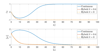
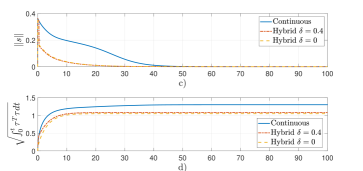
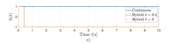
Figure 3: Scenario 1.1: Performance of state-feedback controllers (37), the discontinuous controller (49) with the gap exceeding $\delta=0$, and the hybrid controller (49) with $\delta=0.4$ and. Unwinding phenomenon is observed in the continuous state-feedback controller.

The lack of robustness of the discontinuous controller (49) when the gap exceeding $\delta=0$ in the presence of noise in the quaternion measurement is illustrated in Scenario 1.2 of Table 1. Observe that the presence of noise affects severely the hybrid controller when $\delta=0$, where it shows a chattering phenomenon for the first $9$ $[s]$ reflected in the discrete state $h(t)$ (Fig. 4(e)), causing a delay in the error convergence (Fig. 4(a),(b),(c)) and more energy consumption (Fig. 4(d)). In fact, the hybrid controller with the gap exceeding $\delta=0$ had an increase of $45\%$ in energy consumption than the other controllers. The sensitivity to noise was eliminated when the gap exceeding was changed to $\delta=0.4$. Note that the discrete state makes no jumps despite of the noisy measurements, keeping the discrete state $h=1$ $\forall t\geq 0$ (Fig. 4(e)). Notice that for this scenario, the hybrid controller with the gap exceeding $\delta=0.4$ and the continuous controller have the same behavior, stabilizing $\varepsilon_{0}=1$ at $30$ $[s]$ (Fig.4(a)). The exponential convergence of the equilibrium point $(e,s)=(0_{4\times 1},0_{4\times 1})$ is shown in Fig. 4(b) and Fig. 4(c).

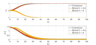
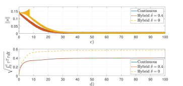
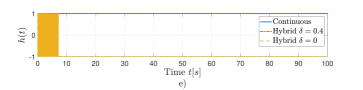
Figure 4: Scenario 1.2: Performance of the continuous state-feedback controllers (37), the discontinuous controller (49) with $\delta=0$, and the hybrid controller (49) with $\delta=0.4$ and respectively. The lack of robustness to noisy measurements in the discontinuous controller is shown.

5.2 Simulation 2: the adaptive hybrid attitude-feedback controller

This simulation shows the behavior of the adaptive hybrid attitude-feedback controller (102) for different values of the gap exceeding and how this behaviour is affected by noisy quaternion measurements and time-varying torque disturbances. The desired trajectory is generated by (31) with the initial condition $q_{d}^{T}(0)=[1,0_{1\times 3}]$ and the desired angular velocity $\omega_{d}=0.1\sin(0.2\pi t)\left[1,1,1\right]^{T}$ $\left[\mathrm{rad}/s\right]$ used in [30]. The initial conditions were $q(0)=[0,0,1,0]^{T}$, $\omega(0)=\bar{u}$ with $\bar{u}=u/\|u\|$ and $u=[1,2,3]^{T}$. The initial discrete state was set $h(0)=1$ for all scenarios. The controller gains (102) were $k_{v}=3$ and, $k_{p}=0.7$, with a filter gain (100), $K_{f}=0.1I_{4}$, and the adaptation gain (103) was $\Gamma=\mathrm{diag}\{1000I_{3},I_{6}\}$. The unknown inertial matrix (8) and the noisy quaternion measurement were the same as in the first simulation. In addition, a torque disturbance $\dot{p}=v$ was added (see (65)), with the initial condition $p(0)=[0.2,-0.1,-0.05]^{T}\ [\mathrm{Nm}]$, where $v=0_{3\times 1}$ for a constant disturbance and $v\in\mathbb{R}^{4}$ whose element is a zero-mean Gauss distribution with variance $0.2$ for a time-varying disturbance (see Table 2).

Table 2: Scenario settings for the the hybrid attitude-feedback controller (102).

Scenario	$\delta$	$q_{m}$	$p(t)$
2.1	$0.9$	$n=0$	$[0.2,-0.1,-0.05]^{T}$
2.2	$0.4$	$n=0$	$[0.2,-0.1,-0.05]^{T}$
2.3	$0.4$	$n\in[0,0.1]$	$[0.2,-0.1,-0.05]^{T}$
2.4	$0.4$	$n=0$	$\dot{p}=v$, $v\in N(0,0.2)$

Scenario 2.1 illustrates the performance of the proposed adaptive hybrid attitude-feedback controller for the gap exceeding $\delta=0.9$ under the noise-free measurements and constant torque disturbance. Due to the large gap exceeding, no jumps were made in spite of the initial angular velocity $\omega(0)$ which favored to stabilizing $\epsilon_{0}=-1$. The norm of $\|e(t)\|$, $\|\nu(t)\|$ and $\|\eta_{2}(t)\|$ are drawn in Figs. 5(a), (b) and (c), respectively. Notice that the estimation error $\|\tilde{\Theta}(t)\|$ remained close to zero (Fig. 5(f)), converging to $0.04$, as ensured by Theorem 11. The generalized torque $\bar{\tau}(t)$ and the torque applied to the spacecraft $\bar{\tau}(t)$ are depicted in Fig. 5(g) and (h).

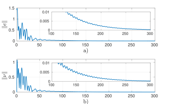
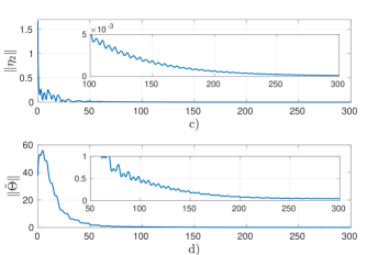
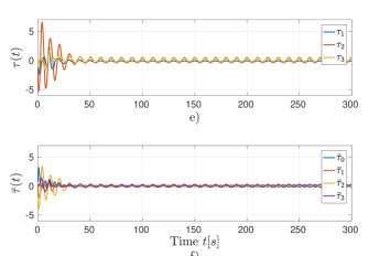
Figure 5: Scenario 2.1: Performance of the adaptive hybrid attitude-feedback controller (102) with a large gap exceeding ($\delta=0.9$).

When the gap exceeding was reduced to $\delta=0.4$, the discrete state $h$ to perform a jump at $t=0.5\ [s]$ due to the initial angular velocity $\omega(0)=\bar{u}$, forcing the attitude to tack a closer path to stabilize $\varepsilon_{0}\to-\hat{1}$ as shown in Figs. 6(a), (b) and (c), where the norm of $\|e\|$, $\|\nu\|$, and $\|\eta_{2}\|$ showed a faster convergence compared to the previous scenario. However, the parameter estimation error $\tilde{\Theta}$ converged to $20$ since the states $e$ and $\nu$ were less exciting compared with the previous situation in the first $50$ $[s]$. Also, notice that the control torque $\tau$ and the generalized torque $\bar{\tau}$ increased slightly in the first $20$ $[s]$ (6(e), (f)).

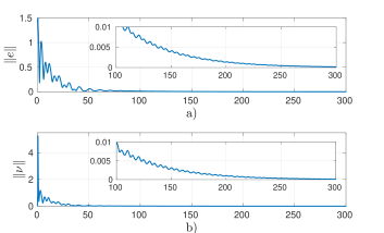
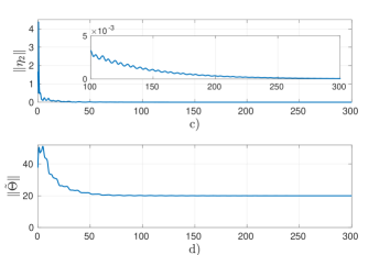
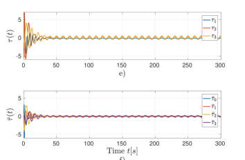
Figure 6: Scenario 2.2: Performance of the adaptive hybrid attitude-feedback controller (102) with a small gap exceeding ($\delta=0.4$).

Scenario 2.3 shows the performance of the adaptive hybrid attitude-feedback controller (102) when the gap exceeding was kept to $\delta=0.4$ and the noisy attitude measurement $q_{m}$ as in Scenario 1.2. Observe from Fig. 7(a), (b) and (c) that the norm of $\|e\|$, $\|\nu\|$ and $\|\eta_{2}\|$ showed an asymptotically decaying behavior as in the previous scenarios, remained bounded by $0.2$, $0.5$ and $0.4$, respectively, after $50\ [s]$. Note that the state $\nu(t)$ was most affected by the attitude noise, because it contains a term in (101) that depends directly on the error $e(t)$ multiplied by the gain $k_{v}$, which amplifies the noise. The estimation error $\tilde{\Theta}$ remained bounded oscillating around $20$ (Fig. 7(d)). Figs. 7(e) and (d) draw the control torques, which increased about $1.0$ $[\textrm{Nm}]$ respect to the previous noise-free scenarios.

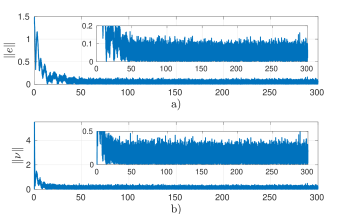
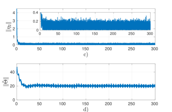
Figure 7: Scenario 2.3: Performance of adaptive controller (102) with gap exceeding $\delta=0.4$ under noisy attitude measurements.

Although the adaptive hybrid attitude-feedback controller (102) is designed for a constant disturbance, the adaptation law can deal with certain time-varying disturbances as illustrated in Scenario 2.4. The time-varying disturbance $p(t)$ is given in Table 2 and displayed in Fig. 8. Likewise, Fig. 9 shows the performance of the adaptive controller. Notice that the norm of the parameter error $\tilde{\Theta}(t)$ converges to $20$ as in Scenario 2.3 where a constant disturbance was used .

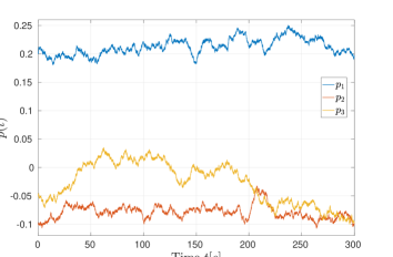
Figure 8: A time-varying torque disturbance $\dot{p}=v$, with the initial condition $p(0)=[0.2,-0.1,-0.05]^{T}\ [\mathrm{Nm}]$ and $v\in\mathbb{R}^{3}$, $v_{i}\in N(0,0.2)$ a Gauss distribution .

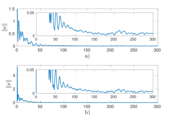
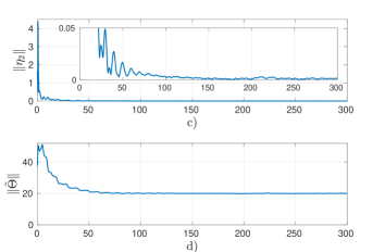
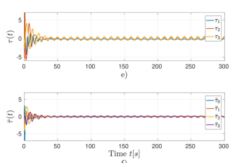
Figure 9: Scenario 2.4: Performance of adaptive controller (102) with gap exceeding $\delta=0.4$ under time-varying torque disturbance $p(t)$.

6 Conclusions

This paper has proposed a novel Lagrangian approach to attitude tracking for rigid spacecraft using unit quaternions. By describing the attitude of a rigid spacecraft by a 4-DOF Lagrangian dynamics with a holonomic constraint imposed by the norm of a unit quaternion and exploring the energy-conservation property of a Lagrangian system, this approach enables to leverage a broad class of tracking control designs for mechanical systems based on energy-shaping methodology to design globally exponentially stable attitude tracking controllers. The salient features of the proposed approach are its capability of using the whole quaternion to design continuous attitude tracking controllers in contrast to using only the vector part of the quaternion reported in the literature, avoiding the topological constraints encountered in the quaternion group. Since the quaternion representation is singularity-free, this approach also avoids the singularity issues in any 3-parameter attitude representation like Euler angles, Rodrigues, or Modified Rodrigues parametrizations.

Using this approach, a state-feedback controller was designed when both the attitude and angular velocity are available for feedback. Then several important issues, such as robustness to noise in quaternion measurements, unknown on-orbit torque disturbances, uncertainty in the inertial matrix, and lack of angular-velocity measurements are addressed by designing a hybrid state-feedback controller, an adaptive hybrid state-feedback controller, and an adaptive hybrid attitude-feedback controller. Global asymptotic stability is established for each controller.

This work was supported in part by CONACyT under grant 253677 and by PAPIIT-UNAM IN112421, and carried out in the National Laboratory of Automobile and Aerospace Engineering LN-INGEA.

Appendix A Proof of Lemma 1

Consider the matrix $Q(\cdot)$ defined as (5). Let $x\in\mathcal{S}^{3}$, then

$$\mathrm{det}\left(Q(x)\right)=\left(x^{T}x\right)^{2}=1.$$

Moreover,

$$Q^{T}(x)Q(x)=Q(x)Q^{T}(x)=(x^{T}x)I_{4}=I_{4}.$$

This shows the property 1.

The property 2 can be verified directly by substitution. Indeed, let $x=\left[x_{0},\ x^{T}_{v}\right]^{T}$ and $y=\left[y_{0},\ y^{T}_{v}\right]^{T}$, with $x_{0},\ y_{0}\in\mathbb{R}$ and $x_{v},y_{v}\in\mathbb{R}^{3}$. Define $J_{v}(x)=x_{0}I_{3}+S(x_{v})$ and $J_{v}(y)=y_{0}I_{3}+S(y_{v})$, then

$$Q (y)Q^{T}(x)=\left[\begin{array}[]{cc}y_{0}&-y^{T}_{v}\\ y_{v}&J_{v}(y)\end{array}\right]\left[\begin{array}[]{cc}x_{0}&x^{T}_{v}\\ -x_{v}&J^{T}_{v}(x)\end{array}\right],$$

$$= \left[\begin{array}[]{cc}y_{0}x_{0}+y^{T}_{v}x_{v}&y_{0}x^{T}_{v}-x_{0}y^{T}_{v}+y^{T}_{v}S(x_{v})\\ x_{0}y_{v}-y_{0}x_{v}-S(y_{v})x_{v}&y_{v}x^{T}_{v}+J_{v}(y)J^{T}_{v}(x)\end{array}\right]$$

$$= \left[\begin{array}[]{cc}y^{T}x&-z^{T}+y^{T}_{v}S(x_{v})\\ z+S(x_{v})y_{v}&\left(y_{v}x^{T}_{v}-x_{v}y^{T}_{v}\right)+S(z)+\left(y^{T}x\right)I_{3}\end{array}\right],$$

where $z=x_{0}y_{v}-y_{0}x_{v}$ and the property of the skew-symmetric operator $S(u)v=-S(v)u$, $\forall u,v\in\mathbb{R}^{3}$ are used. Therefore, the matrix $Q(y)Q^{T}(x)$ is skew-symmetric if and only if $y^{T}x=0$, which verifies the property 3 and 4.

Finally, the properties 5 and 6 can be proved straightforwardly as done in [60] for the matrix $J(\cdot)$.

Appendix B Proof of Lemma 2

The matrix $D(q)$ defined in (9) is symmetric and positive definite follows straightforwardly because $Q(q)\in SO(4)$ for $q\in\mathcal{S}^{3}$ by Property 1 of Lemma 1 for any $m_{0}>0$. This shows the first term of this lemma.

To prove the second term, taking the time derivative of (9) and substituting (11) obtains

$$\dot{D}(q)-2C(q,\dot{q}) = Q(\dot{q})M_{0}Q^{T}(q)+Q(q)M_{0}Q^{T}(\dot{q})$$

$$-2C(q,\dot{q})$$

$$= Q(\dot{q})M_{0}Q^{T}(q)+Q(q)M_{0}Q^{T}(\dot{q})$$

$$+2J(q)S(M\omega)J^{T}(q)$$

$$+2D(q)Q(\dot{q})Q^{T}(q).$$

By the fact that $\dot{q}^{T}q=0$ and Property 4 of the matrix $Q(\cdot)$ in Lemma 1) it follows

$$\dot{D}(q)-2C(q,\dot{q}) = Q(\dot{q})M_{0}Q^{T}(q)+Q(q)M_{0}Q^{T}(\dot{q})$$

$$+2J(q)S(M\omega)J^{T}(q)$$

$$-2D(q)Q(q)Q^{T}(\dot{q}),$$

$$= Q(\dot{q})M_{0}Q^{T}(q)+Q(q)M_{0}Q^{T}(\dot{q})$$

$$+2J(q)S(M\omega)J^{T}(q)$$

$$+2\left(-Q(q)M_{0}Q^{T}(\dot{q})\right),$$

$$= Q(\dot{q})M_{0}Q^{T}(q)-Q(q)M_{0}Q^{T}(\dot{q})$$

$$+2J(q)S(M\omega)J^{T}(q),$$

which is skew symmetric because $J(q)S(M\omega)J^{T}(q)$ is skew symmetric.

Appendix C Proof of Lemma 3

Properties 19 and 2 are proved in this Appendix, the proof of the rest properties was given in [7] for robot manipulators and can be shown for the Lagrangian dynamics (10) following the same procedure as in [7] and is therefore omitted here.

Proof of Property 19: For a vector $u=[u_{1},\;u_{2},\;u_{3}]^{T}\in\mathbb{R}^{3}$ define the map $F\vcentcolon\mathbb{R}^{3}\to\mathbb{R}^{3\times 6}$ as

$$F(u)=\left[\begin{array}[]{cccccc}u_{1}&0&0&0&u_{3}&u_{2}\\ 0&u_{2}&0&u_{3}&0&u_{1}\\ 0&0&u_{3}&u_{2}&u_{1}&0\end{array}\right].$$ (126)

Then, the product $Mu$ can be expressed as $Mu=F(u)\theta$, where $M$ is the inertial matrix in (3) and $\theta$ is defined in (19).

Let $w=J^{T}(q)\dot{q}$, then $\dot{w}=J^{T}(q)\ddot{q}$, therefore, in view of (9), it follows that

$$D(q)\ddot{q} =\left(J(q)MJ^{T}(q)+m_{0}qq^{T}\right)\ddot{q}$$

$$=J(q)F(\dot{w})\theta+m_{0}\left(q^{T}\ddot{q}\right)q.$$ (127)

In addition, by using (9) and Properties 2 and 4 of Lemma 1, the matrix $C(q,\dot{q})$ in (11) is rearranged to

$$C(q,\dot{q}) =-J(q)S(M\omega)J^{T}(q)-D(q)Q(\dot{q})^{T}Q(q)$$

$$=-J(q)S(M\omega)J^{T}(q)+D(q)Q(q)^{T}Q(\dot{q})$$

$$=-J(q)S(M\omega)J^{T}(q)$$

$$\quad+D(q)\left(J(q)J^{T}(\dot{q})+q\dot{q}^{T}\right)$$

$$=-J(q)S(M\omega)J^{T}(q)$$

$$+\left(J(q)MJ^{T}(q)+m_{0}qq^{T}\right)\left(J(q)J^{T}(\dot{q})+q\dot{q}^{T}\right).$$

By properties 4 and 3 of the matrix $J(q)$, it follows that

$$C(q,\dot{q})=-J(q)S(M\omega)J^{T}(q)+J(q)MJ^{T}(\dot{q})+m_{0}q\dot{q}^{T}.$$ (128)

Then, by (128) and (6) the term $C(q,\dot{q})\dot{q}$ can be rewritten as

$$C(q,\dot{q})\dot{q} =\left(-J(q)S(M\omega)J^{T}(q)\right.$$

$$\quad\quad\left.+J(q)MJ^{T}(\dot{q})+m_{0}q\dot{q}^{T}\right)\dot{q}$$

$$=-J(q)S(M\omega)w+m_{0}\left(\dot{q}^{T}\dot{q}\right)q$$

$$=2J(q)S(w)Mw+m_{0}\left(\dot{q}^{T}\dot{q}\right)q$$

$$=2J(q)S(w)F(w)\theta+m_{0}\left(\dot{q}^{T}\dot{q}\right)q.$$ (129)

Now, by adding (127) and (129), it gets

$$D(q)\ddot{q}+C(q,\dot{q})\dot{q} =J(q)F(\dot{w})\theta+m_{0}\left(q^{T}\ddot{q}\right)q$$

$$\quad+2J(q)S(w)F(w)\theta+m_{0}\left(\dot{q}^{T}\dot{q}\right)q$$

$$=m_{0}\left(q^{T}\ddot{q}+\dot{q}^{T}\dot{q}\right)q$$

$$\quad+J(q)\left(F(\dot{w})+2S(w)F(w)\right)\theta$$

$$=\bar{Y}\left(q,\dot{q},\ddot{q}\right)m_{0}+Y\left(q,\dot{q},\ddot{q}\right)\theta$$

which confirms the linear parametrization property 19 of Lemma 3.

Proof of Property 2: The Property 2 can be verified straightforwardly by taking the time derivative $\dot{D}(q)$ from (9) and comparing it with $C(q,\dot{q})+C^{T}(q,\dot{q})$ by using (128).

References

- [1] Morikazu Takegaki and Suguru Arimoto. A new feedback method for dynamic control of manipulators. ASME. J. Dyn. Sys., Meas., Control, 103(2):119–125, 1981.
- [2] Jean-Jacques E Slotine, Weiping Li, et al. Applied nonlinear control, volume 199. Prentice hall Englewood Cliffs, NJ, 1991.
- [3] Hassan K Khalil and Jessy W Grizzle. Nonlinear systems, volume 3. Prentice hall Upper Saddle River, NJ, 2002.
- [4] Dan Koditschek. Natural motion for robot arms. In The 23rd IEEE Conference on Decision and Control, pages 733–735. IEEE, 1984.
- [5] Mark W Spong. Robot dynamics and control, 1989.
- [6] Harry Berghuis and Henk Nijmeijer. Robust control of robots via linear estimated state feedback. IEEE Transactions on Automatic Control, 39(10):2159–2162, 1994.
- [7] Rafael Kelly, Victor Santibáñez Davila, and Julio Antonio Loría Perez. Control of robot manipulators in joint space. Springer Science & Business Media, 2006.
- [8] Romeo Ortega, Julio Antonio Loría Perez, Per Johan Nicklasson, and Hebertt J Sira-Ramirez. Passivity-based control of Euler-Lagrange systems: mechanical, electrical and electromechanical applications. Springer Science & Business Media, 2013.
- [9] Brad Paden and Ravi Panja. Globally asymptotically stable ‘pd+’controller for robot manipulators. International Journal of Control, 47(6):1697–1712, 1988.
- [10] Jean-Jacques E Slotine and Weiping Li. On the adaptive control of robot manipulators. The international journal of robotics research, 6(3):49–59, 1987.
- [11] Romeo Ortega and Mark W Spong. Adaptive motion control of rigid robots: A tutorial. Automatica, 25(6):877–888, 1989.
- [12] Jean-Jacques E Slotine and Weiping Li. Composite adaptive control of robot manipulators. Automatica, 25(4):509–519, 1989.
- [13] Yu Tang and Marco A Arteaga. Adaptive control of robot manipulators based on passivity. IEEE Transactions on Automatic Control, 39(9):1871–1875, 1994.
- [14] Yu Tang. Terminal sliding mode control for rigid robots. Automatica, 34(1):51–56, 1998.
- [15] Yong Feng, Xinghuo Yu, and Zhihong Man. Non-singular terminal sliding mode control of rigid manipulators. Automatica, 38(12):2159–2167, 2002.
- [16] Emmanuel Cruz-Zavala, Emmanuel Nuño, and Jaime A Moreno. Continuous finite-time regulation of euler-lagrange systems via energy shaping. International Journal of Control, 93(12):2931–2940, 2020.
- [17] L-C Fu. Robust adaptive decentralized control of robot manipulators. IEEE Transactions on Automatic Control, 37(1):106–110, 1992.
- [18] Yu Tang, Masayoshi Tomizuka, G Guerrero, and Gustavo Montemayor. Decentralized robust control of mechanical systems. IEEE Transactions on Automatic control, 45(4):771–776, 2000.
- [19] Jie Mei, Wei Ren, and Guangfu Ma. Distributed containment control for lagrangian networks with parametric uncertainties under a directed graph. Automatica, 48(4):653–659, 2012.
- [20] Mark W Spong and Nikhil Chopra. Synchronization of networked lagrangian systems. In Lagrangian and Hamiltonian Methods for Nonlinear Control 2006, pages 47–59. Springer, 2007.
- [21] Soon-Jo Chung, Umair Ahsun, and Jean-Jacques E Slotine. Application of synchronization to formation flying spacecraft: Lagrangian approach. Journal of Guidance, Control, and Dynamics, 32(2):512–526, 2009.
- [22] Jie Mei, Wei Ren, and Guangfu Ma. Distributed coordinated tracking with a dynamic leader for multiple euler-lagrange systems. IEEE Transactions on Automatic Control, 56(6):1415–1421, 2011.
- [23] Francesco Bullo and Richard M Murray. Tracking for fully actuated mechanical systems: a geometric framework. Automatica, 35(1):17–34, 1999.
- [24] Nalin A Chaturvedi, Amit K Sanyal, and N Harris McClamroch. Rigid-body attitude control. IEEE control systems magazine, 31(3):30–51, 2011.
- [25] JT-Y Wen and Kenneth Kreutz-Delgado. The attitude control problem. IEEE Transactions on Automatic control, 36(10):1148–1162, 1991.
- [26] O Egeland and J-M Godhavn. Passivity-based adaptive attitude control of a rigid spacecraft. IEEE Transactions on Automatic Control, 39(4):842–846, 1994.
- [27] Fernando Lizarralde and John T Wen. Attitude control without angular velocity measurement: A passivity approach. IEEE Trans. Autom. Control, 41(3):468–472, Mar. 1996.
- [28] J Thienel and Robert M Sanner. A coupled nonlinear spacecraft attitude controller and observer with an unknown constant gyro bias and gyro noise. IEEE transactions on Automatic Control, 48(11):2011–2015, 2003.
- [29] Wencheng Luo, Yun-Chung Chu, and Keck-Voon Ling. Inverse optimal adaptive control for attitude tracking of spacecraft. IEEE Transactions on Automatic Control, 50(11):1639–1654, 2005.
- [30] Abdelhamid Tayebi. Unit quaternion-based output feedback for the attitude tracking problem. IEEE Transactions on Automatic Control, 53(6):1516–1520, 2008.
- [31] Panagiotis Tsiotras. Further passivity results for the attitude control problem. IEEE Transactions on Automatic Control, 43(11):1597–1600, 1998.
- [32] Maruthi R Akella. Rigid body attitude tracking without angular velocity feedback. Systems & Control Letters, 42(4):321–326, 2001.
- [33] SP Arjun Ram and Maruthi R Akella. Uniform exponential stability result for the rigid-body attitude tracking control problem. Journal of Guidance, Control, and Dynamics, 43(1):39–45, 2020.
- [34] Malcolm D Shuster. A survey of attitude representations. Navigation, 8(9):439–517, 1993.
- [35] Sanjay P Bhat and Dennis S Bernstein. A topological obstruction to continuous global stabilization of rotational motion and the unwinding phenomenon. Systems & Control Letters, 39(1):63–70, 2000.
- [36] Christopher G Mayhew, Ricardo G Sanfelice, and Andrew R Teel. Quaternion-based hybrid control for robust global attitude tracking. IEEE Transactions on Automatic control, 56(11):2555–2566, 2011.
- [37] Daniel E Koditschek. The application of total energy as a lyapunov function for mechanical control systems. Contemporary mathematics, 97:131, 1989.
- [38] Christopher G Mayhew and Andrew R Teel. Synergistic hybrid feedback for global rigid-body attitude tracking on . IEEE Transactions on Automatic Control, 58(11):2730–2742, 2013.
- [39] Soulaimane Berkane, Abdelkader Abdessameud, and Abdelhamid Tayebi. Hybrid global exponential stabilization on so (3). Automatica, 81:279–285, 2017.
- [40] Rafal Wisniewski and Piotr Kulczycki. Rotational motion control of a spacecraft. IEEE Transactions on Automatic Control, 48(4):643–646, 2003.
- [41] Pedro Casau, Christopher G Mayhew, Ricardo G Sanfelice, and Carlos Silvestre. Robust global exponential stabilization on the n-dimensional sphere with applications to trajectory tracking for quadrotors. Automatica, 110:108534, 2019.
- [42] Taeyoung Lee. Global exponential attitude tracking controls on so(3). IEEE Transactions on Automatic Control, 60(10):2837–2842, 2015.
- [43] Christopher G Mayhew, Ricardo G Sanfelice, and Andrew R Teel. Synergistic lyapunov functions and backstepping hybrid feedbacks. In Proceedings of the 2011 American control conference, pages 3203–3208. IEEE, 2011.
- [44] Soulaimane Berkane, Abdelkader Abdessameud, and Abdelhamid Tayebi. Hybrid output feedback for attitude tracking on so(3). IEEE Transactions on Automatic Control, 63(11):3956–3963, 2018.
- [45] O-E Fjellstad and Thor I Fossen. Position and attitude tracking of auv’s: a quaternion feedback approach. IEEE Journal of Oceanic Engineering, 19(4):512–518, 1994.
- [46] Shunan Wu, Gianmarco Radice, Yongsheng Gao, and Zhaowei Sun. Quaternion-based finite time control for spacecraft attitude tracking. Acta Astronautica, 69(1-2):48–58, 2011.
- [47] Fabrizio Caccavale and Luigi Villani. Output feedback control for attitude tracking. Systems & Control Letters, 38(2):91–98, 1999.
- [48] BT Costic, DM Dawson, MS De Queiroz, and Vikram Kapila. Quaternion-based adaptive attitude tracking controller without velocity measurements. Journal of Guidance, Control, and Dynamics, 24(6):1214–1222, 2001.
- [49] E TOMEI. Nonlinear observer and output feedback attitude control of spacecraft. IEEE Transactions on Aerospace and Electronic Systems, 28(4), 1992.
- [50] Thor I Fossen and Svein I Sagatun. Adaptive control of nonlinear systems: A case study of underwater robotic systems. Journal of Robotic Systems, 8(3):393–412, 1991.
- [51] JJE Slotine and MD Di Benedetto. Hamiltonian adaptive control of spacecraft. IEEE Transactions on Automatic Control, 35(7):848–852, 1990.
- [52] H Wong, Marcio S de Queiroz, and Vikram Kapila. Adaptive tracking control using synthesized velocity from attitude measurements. Automatica, 37(6):947–953, 2001.
- [53] Preston Culbertson, Jean-Jacques Slotine, and Mac Schwager. Decentralized adaptive control for collaborative manipulation of rigid bodies. IEEE Transactions on Robotics, 2021.
- [54] Firdaus E Udwadia and Aaron D Schutte. A unified approach to rigid body rotational dynamics and control. Proceedings of the Royal Society A: Mathematical, Physical and Engineering Sciences, 468(2138):395–414, 2012.
- [55] Jonathan Rodriguez, Herman Castañeda, and José Luis Gordillo. Lagrange modeling and navigation based on quaternion for controlling a micro auv under perturbations. Robotics and Autonomous Systems, 124:103408, 2020.
- [56] Firdaus E Udwadia and Aaron D Schutte. An alternative derivation of the quaternion equations of motion for rigid-body rotational dynamics. Journal of Applied Mechanics, 77(4), 2010.
- [57] Karim Sherif, Karin Nachbagauer, and Wolfgang Steiner. On the rotational equations of motion in rigid body dynamics when using euler parameters. Nonlinear dynamics, 81(1):343–352, 2015.
- [58] Taeyoung Lee, Melvin Leok, and N Harris McClamroch. Global formulations of lagrangian and hamiltonian dynamics on manifolds. Springer, 13:31, 2017.
- [59] Firdaus E Udwadia and Aaron D Schutte. Equations of motion for general constrained systems in lagrangian mechanics. Acta mechanica, 213(1):111–129, 2010.
- [60] F Landis Markley and John L Crassidis. Fundamentals of spacecraft attitude determination and control, volume 33. Springer, 2014.
- [61] Shihua Li, Shihong Ding, and Qi Li. Global set stabilization of the spacecraft attitude control problem based on quaternion. International Journal of Robust and Nonlinear Control: IFAC-Affiliated Journal, 20(1):84–105, 2010.
- [62] Yicheng Liu, Tao Zhang, Chengxin Li, and Bin Liang. Robust attitude tracking with exponential convergence. IET Control Theory & Applications, 11(18):3388–3395, 2017.
- [63] John L Junkins and Hanspeter Schaub. Analytical mechanics of space systems. American Institute of Aeronautics and Astronautics, 2009.
- [64] Taeyoung Lee. Exponential stability of an attitude tracking control system on so (3) for large-angle rotational maneuvers. Systems & Control Letters, 61(1):231–237, 2012.
- [65] Haichao Gui and George Vukovich. Global finite-time attitude tracking via quaternion feedback. Systems & Control Letters, 97:176–183, 2016.
- [66] Fumin Zhang, Darren M Dawson, Marcio S de Queiroz, and Warren E Dixon. Global adaptive output feedback tracking control of robot manipulators. IEEE Transactions on Automatic Control, 45(6):1203–1208, 2000.
- [67] Jasim Ahmed, Vincent T Coppola, and Dennis S Bernstein. Adaptive asymptotic tracking of spacecraft attitude motion with inertia matrix identification. Journal of Guidance, Control, and Dynamics, 21(5):684–691, 1998.