Understanding Rare Spurious Correlations in Neural Networks

Abstract

Neural networks are known to use spurious correlations such as background information for classification. While prior work has looked at spurious correlations that are widespread in the training data, in this work, we investigate how sensitive neural networks are to rare spurious correlations, which may be harder to detect and correct, and may lead to privacy leaks. We introduce spurious patterns correlated with a fixed class to a few training examples and find that it takes only a handful of such examples for the network to learn the correlation. Furthermore, these rare spurious correlations also impact accuracy and privacy. We empirically and theoretically analyze different factors involved in rare spurious correlations and propose mitigation methods accordingly. Specifically, we observe that $\ell_{2}$ regularization and adding Gaussian noise to inputs can reduce the undesirable effects.

1 Introduction

Neural networks are known to use spurious patterns for classification. Image classifiers use background as a feature to classify objects (Gururangan et al., 2018; Sagawa et al., 2020; Srivastava et al., 2020; Zhou et al., 2021) often to the detriment of generalization (Nagarajan et al., 2020). For example, Sagawa et al. (2020) show that models trained on the Waterbirds datasetcorrelate waterbirds with backgrounds containing water, and models trained on the CelebA dataset Liu et al. (2018) correlate males with dark hair. In all these cases, spurious patterns are present in a substantial number of training points. The vast majority of waterbirds, for example, are photographed next to the water.

Understanding how and when spurious correlations appear in neural networks is a frontier research problem and remains elusive. In this paper, we study spurious correlations in the context where the appearance of spurious patterns is rare in the training data. Our motivations are three-fold. First, while it is reasonable to expect that widespread spurious correlations in the training data will be learnt, a related question is what happens when these correlations are rare. Understanding if and when they are learnt and how to mitigate them is a first and necessary step before we can understand and mitigate spurious correlations more broadly. Second, rare spurious correlation may inspire us to discover new approaches to mitigate them as traditional approaches such as balancing out groups (Sagawa et al., 2020), subsampling (Idrissi et al., 2021), or data augmentation (Chang et al., 2021) do not apply. Third, rare spurious correlations naturally connect to data privacy. For example, in Leino & Fredrikson (2020), the training set had an image of Tony Blair with a pink background. This led to a classifier that assigned a higher likelihood of the label “Tony Blair” to all images with pink backgrounds. Thus, an adversary could exploit this to infer the existence of “Tony Blair” with a pink background in the training set by by presenting images of other labels with a pink background.

We systematically investigate rare spurious correlations through the following three research questions. First, when do spurious correlations appear, i.e., how many training points with the spurious pattern would cause noticeable spurious correlations? Next, how do rare spurious correlations affect neural networks? Finally, is there any way to mitigate the undesirable effects of rare spurious correlations?

1.1 Overview

We attempt to answer the above questions via both experimental and theoretical approaches. On the experimental side, we introduce spurious correlations into real image datasets by turning a few training data into spurious examples, i.e., adding a spurious pattern to a training image from a target class. We then train a neural network on the modified dataset and measure the strength of the correlation between the spurious pattern and the target class in the network. On the theoretical side, we design a toy mathematical model that enables quantitative analysis on different factors (e.g., the fraction of spurious examples, the signal-to-noise ratio, etc.) of rare spurious correlations. Our responses to the three research questions are summarized in the following.

Rare spurious correlations appear even when the number of spurious samples is small. Empirically, we define a spurious score to measure the amount of spurious correlations. We find that the spurious score of a neural network trained with only $1$ spurious examples out of 60,000 training samples can be significantly higher than that of the baseline. A visualization of the trained model also reveals that the network’s weights may be significantly affected by the spurious pattern. In our theoretical model, we further discover that there is a sharp phase transition of spurious correlations from no spurious training example to a non-zero fraction of spurious training examples. Together, these findings provide a strong evidence that spurious correlations can be learnt even when the number of spurious samples is extremely small.

Rare spurious correlations affect both the privacy and test accuracy. We analyze the privacy issue of rare spurious correlations via the membership inference attack (Shokri et al., 2017; Yeom et al., 2017), which measures the privacy level according to the hardness of distinguishing training samples from testing samples. We observe that the spurious training examples are more vulnerable to membership inference attacks. That is, it is easy for an adversary to tell whether a spurious sample is from the training set. This apparently raises serious concerns for privacy Leino & Fredrikson (2020) and fairness to small groups Izzo et al. (2021).

We examine the effect of rare spurious correlations on test accuracy through two accuracy notions: the clean test accuracy, which uses the original test examples, and the spurious test accuracy, which adds the spurious pattern to all the test examples. Both empirically and theoretically, we find that clean test accuracy does not change too much while the spurious test accuracy significantly drops in the face of rare spurious correlations. This suggests that the undesirable effect of spurious correlations could be more serious when there is a distribution shift toward having more spurious samples.

Methods to mitigate the undesirable effects of rare spurious correlations. Finally, inspired by our theoretical analysis, we examine three regularization methods to reduce the privacy and test accuracy concerns: adding Gaussian noises to the input samples, $\ell_{2}$ regularization (or equivalently, weight decay), and gradient clipping. We find that adding Gaussian noise and $\ell_{2}$ regularization effectively reduce spurious score and improve spurious test accuracy. Meanwhile, not all regularization methods could reduce the effects of rare spurious correlations, e.g., gradient clipping. Our findings suggest that rare spurious correlations should be dealt differently from traditional privacy issues. We post it as a future research problem to deepen the understanding of how to mitigate rare spurious correlations.

Concluding remarks. The study of spurious correlations is crucial for a better understanding of neural networks. In this work, we take a step forward by looking into a special (but necessary) case of spurious correlations where the appearance of spurious examples is rare. We demonstrate both experimentally and theoretically when and how rare spurious correlations appear and what undesirable consequences are. While we propose a few methods to mitigate rare spurious correlations, we emphasize that there is still a lot to explore, and we believe the study of rare spurious correlations could serve as a guide for understanding the more general cases.

2 Preliminaries

We focus on studying spurious correlations in the image classification context. Here, we briefly introduce the notations and terminologies used in the rest of the paper. Let $\mathcal{X}$ be an input space and let $\mathcal{Y}$ be a label space. At the training time, we are given a set of examples $\{(\mathbf{x}_{i},y_{i})\}_{i\in\{1,\dots,n\}}$ sampled from a distribution $\mathcal{D}_{\text{train}}$, where each $\mathbf{x}_{i}\in\mathcal{X}$ is associated with a label $y_{i}\in\mathcal{Y}$. At the testing time, we evaluate the network on test examples drawn from a test distribution. We consider two types of test distribution: the clean test distribution $\mathcal{D}_{\text{ctest}}$ and the spurious test distribution $\mathcal{D}_{\text{stest}}$. Their formal definitions will be mentioned in the related sections.

Spurious correlation. A spurious correlation refers to the relationship between two variables in which they are correlated but not causally related. We build on top of the framework used in Nagarajan et al. (2020) to study spurious correlations. Concretely, the input $\mathbf{x}$ is modeled as the output of a feature map $\Phi_{\mathcal{X}}$ from the feature space $\mathcal{X}_{\text{inv}}\times\mathcal{X}_{\text{sp}}$ to the input space $\mathcal{X}$. Here, $\mathcal{X}_{\text{inv}}$ is the invariant feature space containing the features that causally determine the label and $\mathcal{X}_{\text{sp}}$ which is the spurious feature space that accommodates spurious features. Finally, $\Phi_{\mathcal{X}}:\mathcal{X}_{\text{inv}}\times\mathcal{X}_{\text{sp}}\to\mathcal{X}$ is the function that maps an feature pair $(\mathbf{x}_{\text{inv}},\mathbf{x}_{\text{sp}})$ to an input $\mathbf{x}$ and $\Phi_{\mathcal{Y}}:\mathcal{X}_{\text{inv}}\to\mathcal{Y}$ is a function that maps the invariant feature $\mathbf{x}_{\text{inv}}$ to a label. Namely, an example $(\mathbf{x},y)$ is generated by $(\mathbf{x}_{\text{inv}},\mathbf{x}_{\text{sp}})$ via $\mathbf{x}=\Phi_{\mathcal{X}}(\mathbf{x}_{\text{inv}},\mathbf{x}_{\text{sp}})$ and $y=\Phi_{\mathcal{Y}}(\mathbf{x}_{\text{inv}})$. Without loss of generality, the zero vector in $\mathcal{X}_{\text{sp}}$, i.e., $0\in\mathcal{X}_{\text{sp}}$, refers to “no spurious feature” and for any nonzero $\mathbf{x}_{\text{sp}}$ we call $\Phi(\mathbf{x}_{\text{inv}},\mathbf{x}_{\text{sp}})-\Phi(\mathbf{x}_{\text{inv}},0)$ a spurious pattern. We focus on the case of having a fixed spurious feature $\mathbf{x}_{\text{sp}}$ and leave it as a future direction to study the more general scenarios where there are multiple spurious features.

Rare spurious correlation. Following the setting introduced in the previous paragraph, an input distribution $\mathcal{D}$ over $\mathcal{X}$ is induced by a distribution $\mathcal{D}_{\text{feature}}$ over the feature space $\mathcal{X}_{\text{inv}}\times\mathcal{X}_{\text{sp}}$, i.e., to get a sample from $\mathcal{D}$, one first samples $(\mathbf{x}_{\text{inv}},\mathbf{x}_{\text{sp}})$ from $\mathcal{D}_{\text{feature}}$ and outputs $(\mathbf{x},y)$ with $\mathbf{x}=\Phi_{\mathcal{X}}(\mathbf{x}_{\text{inv}},\mathbf{x}_{\text{sp}})$ and $y=\Phi_{\mathcal{Y}}(\mathbf{x}_{\text{inv}})$. Now, we are able to formally discuss the rareness of spurious correlations by defining the spurious frequency of $\mathcal{D}$ as $\gamma:=\Pr_{(\mathbf{x}_{\text{inv}},\mathbf{x}_{\text{sp}})\sim\mathcal{D}_{\text{feature}}}[\mathbf{x}_{\text{sp}}\neq 0]$.

Two simple models for spurious correlations. In general, $\Phi_{\mathcal{X}}$ could be complicated and makes it difficult to detect the appearance of spurious correlations. Here, we consider two simple instantiations of $\Phi_{\mathcal{X}}$ and demonstrate that undesirable learning outcomes already appear even in these simplified settings. First, the overlapping model (used in Sec. 3) where the spurious feature is put on top of the invariant feature, i.e., $\mathcal{X}=\mathcal{X}_{\text{inv}}=\mathcal{X}_{\text{sp}}$ and $\Phi_{\mathcal{X}}(\mathbf{x}_{\text{inv}},\mathbf{x}_{\text{sp}})=\mathbf{x}_{\text{inv}}+\mathbf{x}_{\text{sp}}$ or $\Phi_{\mathcal{X}}(\mathbf{x}_{\text{inv}},\mathbf{x}_{\text{sp}})=clip(\mathbf{x}_{\text{inv}}+\mathbf{x}_{\text{sp}})$ where $clip$ is a function that truncates an input pixel when its value exceeds a certain range. Second, the concatenate model (used in Sec. 5) where the spurious feature is concatenated to the invariant feature, i.e., $\mathcal{X}=\mathcal{X}_{\text{inv}}\times\mathcal{X}_{\text{sp}}$ and $\Phi_{\mathcal{X}}(\mathbf{x}_{\text{inv}},\mathbf{x}_{\text{sp}})=(\mathbf{x}_{\text{inv}},\mathbf{x}_{\text{sp}})$.

3 Rare Spurious Correlations are Learnt by Neural Networks

We start with an empirical study of rare spurious correlations in neural networks. We train a neural network using a modified training dataset given by the overlapping model where a spurious pattern is added to a few training examples with the same label (target class). We then analyze the effect of these spurious training examples through three difference angles: (i) a quantitative analysis on the appearance of spurious correlations via an empirical measure, spurious score, (ii) a qualitative analysis on the appearance of spurious correlations through visualizing the network weights, and (iii) an analysis on the consequences of rare spurious correlations in terms of privacy and test accuracy.

3.1 Introducing spurious examples to networks

As we don’t have access to the underlying ground-truth feature of an empirical data, we artificially introduce spurious features into the training dataset. Concretely, given a dataset (e.g., MNIST), we treat each training example $\mathbf{x}$ as an invariant feature. Next, we pick a target class $c_{\text{tar}}$ (e.g., the zero class), a spurious pattern $\mathbf{x}_{\text{sp}}$ (e.g., a yellow square at the top-left corner), and a mapping $\Phi_{\mathcal{X}}$ that combines a training example with the spurious pattern. Finally, we randomly select $n$ training examples $\mathbf{x}_{1},\dots,\mathbf{x}_{n}$ from the target class $c_{\text{tar}}$ and replace these examples with $\Phi_{\mathcal{X}}(\mathbf{x}_{i},\mathbf{x}_{\text{sp}})$ for each $i=1,\dots,n$. See Fig. 1 and the following paragraphs for a detailed specification of our experiments.

Datasets & the target class $c_{\text{tar}}$. We consider three commonly used image datasets: MNIST (LeCun, 1998), Fashion (Xiao et al., 2017), and CIFAR10 (Krizhevsky & Hinton, 2009). MNIST and Fashion have $60,000$ training examples, and CIFAR10 has $50,000$. We set the first two classes of each dataset as the target class ($c_{\text{tar}}=\{0,1\}$), which are zero and one for MNIST, T-shirt/top, and trouser for Fashion, and airplane and automobile for CIFAR10. See Sec. D.1 for more experimental details.

Spurious patterns $\mathbf{x}_{\text{sp}}$. We consider seven different spurious patterns (Fig. 1) for this study. The patterns small 1 (S1), small 2 (S2), and small 3 (S3) are designed to test if a neural network can learn the correlations between small patterns and the target class. The patterns random 1 (R1), random 2 (R2), and random 3 (R3) are patterns with each pixel value being uniformly random sampled from $[0,r]$, where $r=0.25,0.5,1.0$ (we sample the pattern once and fix it throughout each experiment). We study whether a network learns to correlate random noise with a target class. In addition, by comparing random patterns with these small patterns, we can understand the impact of localized and dispersed spurious patterns. Lastly, the pattern core (Inv) is designed for MNIST with $c_{\text{tar}}=0$ to understand what would happen if the spurious pattern overlaps with the core feature of another class.

The choice of the combination function $\Phi_{\mathcal{X}}$. The function $\Phi_{\mathcal{X}}$ combines the original example $\mathbf{x}$ with the spurious pattern $\mathbf{x}_{\text{sp}}$ into a spurious example. For simplicity, we consider the overlapping model where $\Phi_{\mathcal{X}}$ directly adds the spurious pattern $\mathbf{x}_{\text{sp}}$ onto the original example $\mathbf{x}$ and then clips the value of each pixel to $[0,1]$, i.e., $\Phi_{\mathcal{X}}(\mathbf{x},\mathbf{x}_{\text{sp}})=clip_{[0,1]}(\mathbf{x}+\mathbf{x}_{\text{sp}})$.

The number of spurious examples. For MNIST and Fashion, we randomly insert the spurious pattern to $n=0,1,3,5,10,20,100,2000$, and $5000$ training examples labeled as the target class $c_{\text{tar}}$. These training examples inserted with a spurious pattern are called spurious examples. For CIFAR10, we consider datasets with $n=0,1,3,5,10,20,100$, $500$, and $1000$ spurious examples. Note that $0$ spurious example means the original training set is not modified.

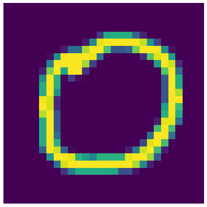
(a) original

(b) S1

(c) S2

(d) S3

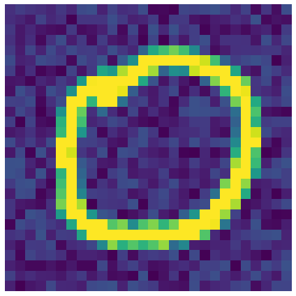
(e) R1

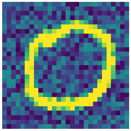
(f) R2

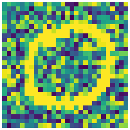
(g) R3

(h) Inv

Figure 1: Different spurious patterns considered in the experiment.

3.2 Quantitative analysis: spurious score

To evaluate the strength of spurious correlations in a neural network, we design an empirical quantitative measure, spurious score, as follows. Let $f_{c}(\mathbf{x})$ be the neural network’s predicted probability of an example $\mathbf{x}$ belonging to class $c$. Intuitively, the larger the prediction difference $f_{c_{\text{tar}}}(\mathbf{x})-f_{c_{\text{tar}}}(\Phi_{\mathcal{X}}(\mathbf{x},\mathbf{x}_{\text{sp}}))$ is, the stronger spurious correlations the neural network $f$ had learned. To quantify the effect of spurious correlations, we measure how frequently the prediction difference of the test examples exceed a certain threshold. Formally, let $\epsilon>0$, we define the $\epsilon$-spurious score as the fraction of test example $\mathbf{x}$ that satisfies

$$f_{c_{\text{tar}}}(\Phi_{\mathcal{X}}(\mathbf{x},\mathbf{x}_{\text{sp}}))-f_{c_{\text{tar}}}(\mathbf{x})>\epsilon\,.$$ (1)

In other words, spurious score measures the portion of test examples that get an non-trivial increase in the predicted probability of the target class $c_{\text{tar}}$ when the spurious pattern is presented.

We make three remarks on the definition of spurious score. First, as we don’t have any prior knowledge on the structure of $f$, we use the fraction of test examples satisfying Eq. 1 as opposed to other function of $f_{c_{\text{tar}}}(\Phi_{\mathcal{X}}(\mathbf{x},\mathbf{x}_{\text{sp}}))-f_{c_{\text{tar}}}(\mathbf{x})$ (e.g., taking average) to avoid non-monotone or unexplainable scaling. Second, the choice of the threshold $\epsilon$ is to avoid numerical errors to affect the result. In our experiment, we pick $\epsilon=1/(\#\text{classes})$ (e.g., in MNIST we pick $\epsilon=1/10$) and empirically similar conclusions can be made with other choices of $\epsilon$. Finally, we point out that spurious score captures the privacy concern raised by the “Tony Blair” example mentioned in the introduction.

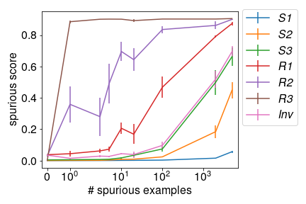
(a) MNIST, $c_{\text{tar}}=0$

(b) Fashion, $c_{\text{tar}}=0$

(c) CIFAR10, $c_{\text{tar}}=0$

Figure 2: Each figure shows the mean and standard error of the spurious scores on three datasets, MNIST, Fashion, and CIFAR10, $c_{\text{tar}}=0$, and different numbers of spurious examples.

Empirical findings. We repeat the measurement of spurious scores on five neural networks trained with different random seeds. Fig. 2 shows the spurious scores for each dataset and pattern as a function of the number of spurious examples. Starting with the random pattern R3, we see that the spurious scores increase significantly from zero to three spurious examples in all six cases (three datasets and two target classes). This shows that neural networks can learn rare spurious correlations with as little as one to three spurious examples. Since all three datasets have $50,000$ or more training examples, it is surprising that the networks learn a strong correlation with extremely small amount of spurious examples. The result for other $c_{\text{tar}}$ are similar and can be found in App. D.

A closer look at Fig. 2 reveals a few other interesting observations. First, comparing the small and random patterns, we see that random patterns generally have a higher spurious score. This suggests that dispersed patterns that are spread out over multiple pixels may be more easily learnt than more concentrated ones. Second, spurious correlations are learnt even for Inv, on $c_{\text{tar}}=0$ and MNIST (recall that Inv is designed to be similar to the core feature of class one.) This suggests that spurious correlations may be learnt even when the pattern overlaps with the foreground. Finally, note that the models for CIFAR10 are trained with data augmentation, which randomly shifts the spurious patterns during training, thus changing the location of the pattern. This suggests that these patterns can be learnt regardless of data augmentation.

3.3 Qualitative analysis: visualizing network weights

We visualize the changes training with spurious examples can bring to the weights of a neural network. We consider an MLP architecture and pattern S3 on MNIST, and look at the network’s weights from the input layer to the first hidden layer. We visualize the importance of each pixel by plotting the maximum weight (among all weights) on an out-going edge from this pixel. Fig. 3 shows the importance plots for models trained with different numbers of spurious examples.

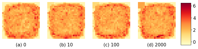
Figure 3: The importance of each pixel during the classification using an MLP trained on MNIST. Each pixel in the figure corresponds to a neuron of the input layer. The value of each pixel in the figure shows the maximum weight among all the weights that go out of the corresponding neuron from the input layer to the first hidden layer. The darker the color is, the larger the maximum weight is, which translates to the higher importance of the pixel during classification. The MLPs are trained on datasets with $0$, $10$, $100$, and $2000$ spurious examples on MNIST.

On the figure with zero spurious examples (Fig. 3 (a)), we see that the pixels in the top left corner are not important at all. When the number of spurious examples goes up, the values in the top left corner become larger (darker in the figure). This means that the pixels in the top left corner are gaining in importance, thus illustrating how they affect the network.

3.4 Natural Rare Spurious Correlations

Another question is whether rare spurious correlations are also learnt on real (natural) data. To answer this question, we conduct an experiment focusing on natural spurious patterns using the NICO++ (Zhang et al., 2022) dataset, which is designed for studying non-I.I.D. image classification There are two labels of each image in the dataset: an object class (e.g., airplane) and the context (e.g., autumn). The context can then serve as a source of spurious features: if a context only appears with the same class during the training stage (e.g., autumn context only shows up when the concept is airplane), then the algorithm might think the context is causally related to the classification of the object class (e.g., classifying a bear in the autumn context as an airplane).

The NICO++ dataset consists of $55,838$ training images, sixty classes and six contexts, including autumn, dim, grass, outdoor, rock, and water. We split the dataset seven to three as the training and testing set. For each experiment, we use an object-context pair as an invariant-spurious pair for studying rare spurious correlations. For one trial of our experiment, we pick a context (i.e., a spurious feature) and remove all the appearance of this context in the training examples. To introduce spurious training examples, we select an object class as the target class and add a number of examples that are labeled with the target class and this context. We use the ImageNet pretrained ResNet50 from torchvision and train twenty epochs on this modified training set. During testing, we collect all testing examples that do not belong to the spurious class but are under the spurious context and measure how many of these examples are predicted as the spurious class.

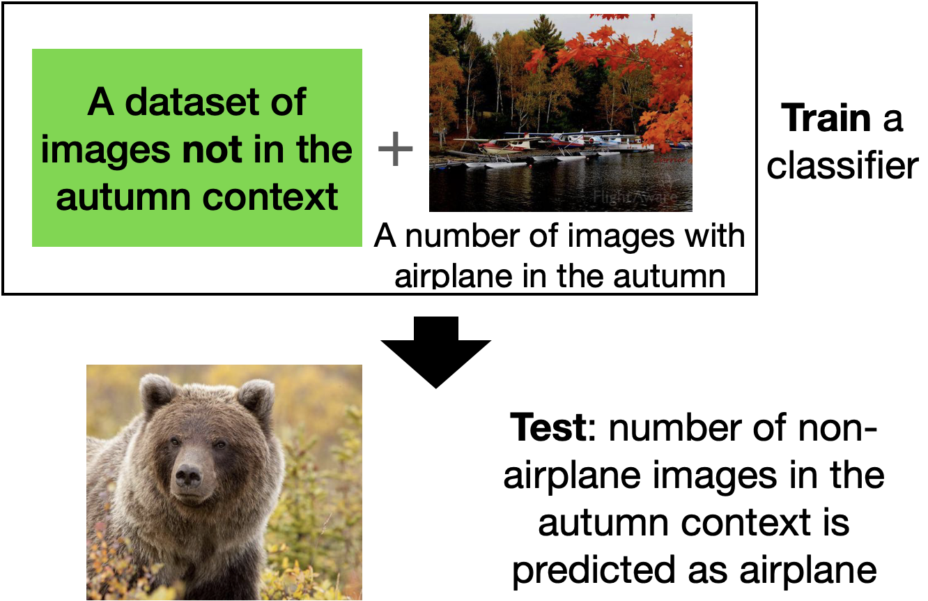
(a) An illustration of the experiment setup.

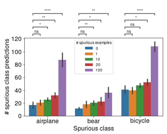
(b) Spurious context: autumn

Figure 4: (b) The number of non-spurious test examples that get predicted as the spurious class. We conduct Welch’s t-test (Welch, 1947) on the number of spurious class predictions between the model trained without spurious examples and models trained with different number of spurious examples. The notations for the p-values: ns$:0.05<p\leq 1.$, *$:10^{-2}<p\leq 0.05$, **$:10^{-3}<p\leq 10^{-2}$, ***$:10^{-4}<p\leq 10^{-3}$, ****$:p\leq 10^{-4}$.

Results. The experiments are repeated five times with different numbers of spurious examples in the training set and the results are in Fig. 4(b). In Sec. E.5, we show the results of two other spurious contexts, dim and grass, which also supports our conclusion. in total, we run a total of nine trials and five of them are significantly affected by just ten spurious training examples (which is less than $0.02$% in the whole training examples). This suggests that rare spurious correlations also occur when the spurious features are natural.

4 Consequences of rare spurious correlations

In the previous analysis, we demonstrated that spurious correlations appear quantitatively and qualitatively in neural networks even when the number of spurious examples is small. Now, we investigate the potentially undesirable effects through the lens of privacy and test accuracy. In this section, the results for MNIST are similar to Fashion and CIFAR10 and are deferred to App. D.

Privacy. We evaluate the privacy of a neural network (the target model) through membership inference attack. We follow the setup for black-box membership inference attack (Shokri et al., 2017; Yeom et al., 2017). We record how well an attack model can distinguish whether an example is from the training or testing set using the output of the target model (equivalently to a binary classification problem). If the attack model has a high accuracy, this means that the target model is leaking out information from the training (private) data. The experiment is repeated ten times with their test accuracy recorded. For more detailed setup, please refer to Sec. D.2.

Results on membership inference attack. Fig. 5 shows the mean and standard error of the attack model’s test accuracy on all test examples and spurious examples. We see that the accuracies on spurious examples is generally higher when the number of spurious examples are small, which means that spurious examples are more vulnerable to membership inference attacks when appeared rarely. Although membership inference attack is a different measure for privacy than spurious score, it can be a corroboration evidence that supports the fact that privacy is leaked from spurious examples.

Test accuracy. We measure two types of test accuracy on neural networks trained on different number of spurious examples. The clean test accuracy measures the accuracy of the trained model on the original test data. The spurious test accuracy simulates the case where there is a distribution shift during the test time. Formally, spurious test accuracy is defined as the accuracy on a new test dataset constructed by adding spurious features to all the test examples with a label different from $c_{\text{tar}}$.

Results on clean test accuracy. We observe that the change in clean test accuracy in our experiments is small. Across all the models trained in Fig. 2, the minimum, maximum, average, and standard deviation of the test accuracy for each dataset are: MNIST: $(.976,.983,.980,.001)$, Fashion: $(.859,.903,.890,.010)$, and CIFAR10: $(.876,.893,.886,.003)$.

Results on spurious test accuracy. The results are shown in Fig. 6. We have two observations. First, we see that there are already some accuracy drop even when spurious test accuracy is evaluated on models trained on zero spurious examples. This means that these models are not robust to the existence of spurious features. This phenomena is prominent for spurious patterns with larger norm such as R3. Second, we see that spurious test accuracies start to drop even more at around $10$ to $100$ spurious examples. This indicates that even with $.01$ % to $.001$ % of the overall training data filled with spurious examples of a certain class, the robustness to spurious features can drop significantly.

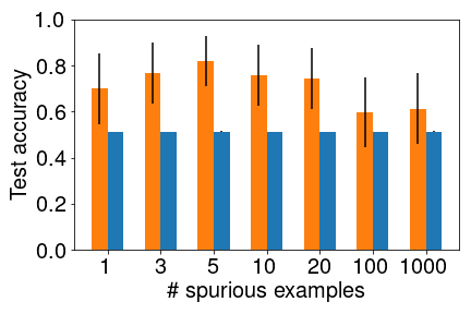
(a) MNIST, $c_{\text{tar}}=0$

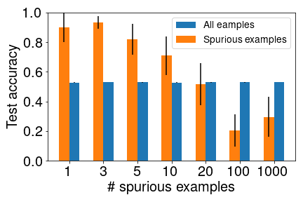
(b) Fashion, $c_{\text{tar}}=0$

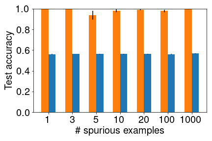
(c) CIFAR10, $c_{\text{tar}}=0$

Figure 5: The test accuracy of the membership inference attack model on all examples vs. spurious examples. See Sec. E.3 for all results.

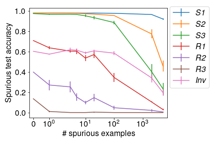
(a) MNIST, $c_{\text{tar}}=0$

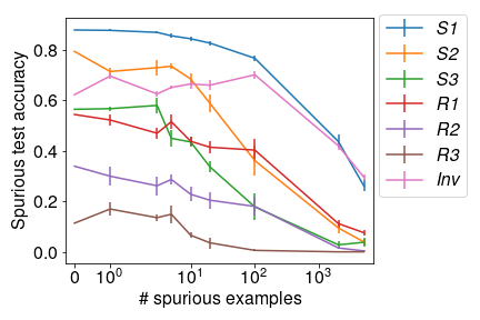
(b) Fashion, $c_{\text{tar}}=0$

(c) CIFAR10, $c_{\text{tar}}=0$

Figure 6: The mean and standard error of the spurious test accuracy under different number of spurious examples. See Sec. E.4 for all results.

Discussion. Our experimental results suggest that neural networks are highly sensitive to very small amounts of spurious training data. Furthermore, the learnt rare spurious correlations cause undesirable effects on privacy and test accuracy. Easy learning of rare spurious correlations can lead to privacy issues (Leino & Fredrikson, 2020) – where an adversary may infer the presence of a confidential image in a training dataset based on output probabilities. It also raises fairness concerns as a neural network can draw spurious conclusions about a minority group if a small number of subjects from this group are present in the training set (Izzo et al., 2021). We recommend to test and audit neural networks thoroughly before deployment in these applications.

Beyond the empirical analysis explained in this section, we also explore how other factors such as the strength of spurious patterns, network architectures, and optimization methods, affect spurious correlations. We find that one cannot remove rare spurious correlations by simply tuning these parameters. We also observe that neural networks with more parameters may not always learn spurious correlations more easily, which is counter to Sagawa et al. (2020)’s observation. The detailed results and discussions are provided in App. B.

5 Theoretical Understanding

In this section, we devise a mathematical model to study rare spurious correlations. The theoretical analysis not only provides an unifying understanding to explain the experimental findings but also inspires us to propose methods to reduce the undesirable effects of rare spurious correlations in Sec. 6. We emphasize that the purpose of the theoretical analysis is to capture the key factors in rare spurious correlations and we leave it as a future research direction to further deepen the theoretical study.

To avoid unnecessary mathematical complications, we make two simplifications in our theoretical analysis: (i) we focus on the concatenate model and (ii) the learning algorithm is linear regression with mean square loss. For (i), we argue that this is the simplest scenario of spurious correlations and hence it is a necessary step before we understand general spurious correlations. While the experiments in Sec. 3 work in the overlapping model, we believe that the high level messages of our theoretical analysis would extend to there as well as other more general scenarios. For (ii), we pick a simpler learning algorithm in order to have an analytical characterization of the algorithm’s performance. This is because we aim to have an understanding of how the different factors (e.g., the fraction of spurious inputs, the strength of spurious feature, etc.) of spurious correlations play a role.

5.1 A theoretical model to study rare spurious correlations

We consider a binary classification task to model the appearance of rare spurious correlations. Let $\mathcal{X}=\mathcal{X}_{\text{inv}}\times\mathcal{X}_{\text{sp}}$ be an input vector space and let $\mathcal{Y}=\{-1,1\}$ be a label space. Let $\gamma\in[0,1]$ be the parameter for the fraction of spurious samples, let $\mathbf{x}_{-},\mathbf{x}_{+}\in\mathcal{X}_{\text{inv}}$ be the invariant features of the two classes, let $\mathbf{x}_{\text{sp}}\in\mathcal{X}_{\text{sp}}$ be the spurious feature, and let $\sigma_{\text{inv}}^{2},\sigma_{\text{sp}}^{2}>0$ be the parameters for the variance along $\mathcal{X}_{\text{inv}}$ and $\mathcal{X}_{\text{sp}}$ respectively. Finally, the target class is $+$, i.e., $c_{tar}=+$. We postpone the formal definitions of the training distribution $\mathcal{D}_{\text{train}}$, the clean text distribution $\mathcal{D}_{\text{ctest}}$, and the spurious test distribution $\mathcal{D}_{\text{stest}}$ to App. A. See also Fig. 7 for some pictorial examples.

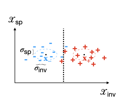
(a) $\gamma=0$

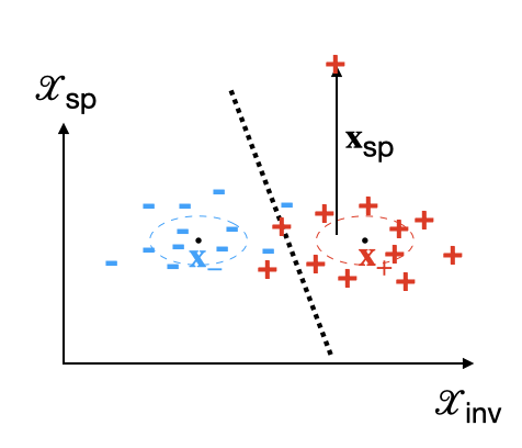
(b) $\gamma>0$

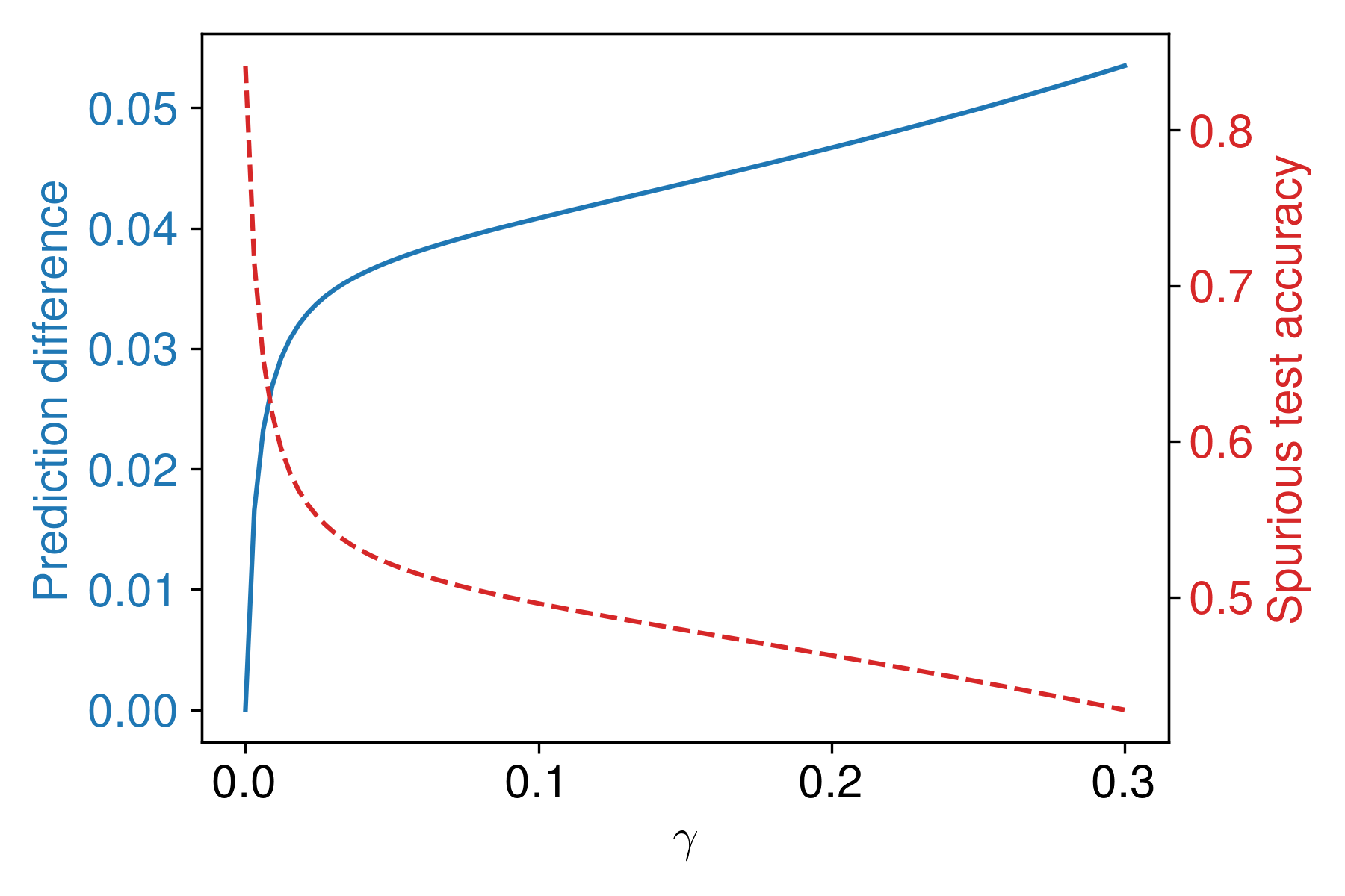
(c) Phase transitions

Figure 7: Examples of the training distribution $\mathcal{D}_{\text{train}}$ and phase transitions in our theoretical model. (a)-(b) With equal probability a training example is sampled from either $\mathcal{N}(\mathbf{x}_{+},\sigma_{\text{inv}}I_{\text{inv}}+\sigma_{\text{sp}}I_{\text{sp}})$ or $\mathcal{N}(\mathbf{x}_{-},\sigma_{\text{inv}}I_{\text{inv}}+\sigma_{\text{sp}}I_{\text{sp}})$. With probability $\gamma$, a $+$ sample will be concatenated with the spurious pattern $\mathbf{x}_{\text{sp}}$. The dotted line is the decision boundary of the optimal classifier. (c) Both the spurious test accuracy and the prediction difference exhibit a phase transition at $\gamma=0$.

5.2 Analysis for linear regression with mean square loss and $\ell_{2}$ regularization

In this paper, we analyze our theoretical model in the setting of linear regression with $\ell_{2}$ loss. We analytically derive the test accuracy and the prediction difference $f_{c_{\text{tar}}}(\Phi_{\mathcal{X}}(\mathbf{x},\mathbf{x}_{\text{sp}}))-f_{c_{\text{tar}}}(\mathbf{x})$ in App. A and here we present our observations. Here, we study the prediction difference as a proxy for the spurious score since the latter is always either $0$ or $1$ for a linear classifier under our model.

Observation 1: A phase transition of spurious test accuracy and prediction difference at $\gamma=0$. Our theoretical analysis first suggests that there is a phase transition of the spurious test accuracy and the prediction difference spurious score at $\gamma=0$, i.e., there is an sharp growth/decay within an interval near $\gamma=0$. The phase transition matches our previous experimental studies discussed in Sec. 3. This indicates that the effect of spurious correlations is spontaneous rather than gradual. To be more quantitative, the phase transition takes place when the signal-to-noise ratio of spurious feature, i.e., $\|\mathbf{x}_{\text{sp}}\|_{2}^{2}/\sigma_{\text{sp}}^{2}$, is large (see App. A for details). This further suggests us to increase the variance in the spurious dimension and leads to our next two observations.

Observation 2: adding Gaussian noises lowers spurious score. The previous observation on the importance of spurious signal-to-noise ratio $\|\mathbf{x}_{\text{sp}}\|_{2}^{2}/\sigma_{\text{sp}}^{2}$ immediately suggests us to add Gaussian noises to the input data to lower $\|\mathbf{x}_{\text{sp}}\|_{2}^{2}/\sigma_{\text{sp}}^{2}$. Indeed, the prediction difference becomes smaller in most parameter regimes, however, both the clean test accuracy and the spurious test accuracy decrease. Intuitively, the effect of adding noises is to mix the invariant feature with the spurious feature and the decrease of test accuracy is as expected. Thus, to simultaneously lower prediction difference and improve test accuracy, one needs to detect the spurious feature in some ways.

Observation 3: $\ell_{2}$ regularization improves test accuracy and lowers spurious score. Finally, our theoretical analysis reveals that there are two parameter regimes where adding $\ell_{2}$ regularization to linear regression can improves accuracy and lowers the prediction difference. First, when $\sigma_{\text{inv}}^{2}$ is small, $\gamma$ is small, and the spurious signal-to-noise ratio $\|\mathbf{x}_{\text{sp}}\|_{2}^{2}/\sigma_{\text{sp}}^{2}$ is large. Second, when $\sigma_{\text{inv}}^{2}$ is large and both $\gamma$ and $\|\mathbf{x}_{\text{sp}}\|_{2}^{2}/\sigma_{\text{sp}}^{2}$ are mild. Intuitively, $\ell_{2}$ regularization suppresses the use of features that only appears on a small number of training examples.

Discussion. Our theoretical analysis quantitatively demonstrates the phase transition of spurious correlations at $\gamma=0$ and the importance of the spurious signal-to-noise ratio $\|\mathbf{x}_{\text{sp}}\|_{2}^{2}/\sigma_{\text{sp}}^{2}$. This not only coincides with our empirical observation in Sec. 3 but also suggests future directions to mitigate rare spurious correlations. Specifically, one general approach to reduce the undesirable effects of rare spurious correlations would be designing learning algorithms that projects the input into a feature space that has a low spurious signal-to-noise ratio.

6 Mitigation of Rare Spurious Correlation

Prior work uses group rebalancing (Idrissi et al., 2021; Sagawa et al., 2020; 2019; Kulynych et al., 2022), data augmentation (Chang et al., 2021) or learning invariant classifier (Arjovsky et al., 2019) to mitigate spurious correlations. However, these methods usually requires additional information on what the spurious feature is, and in rare spurious correlations, identifying the spurious feature can be hard. Thus, we may require different techniques.

Our theoretical result suggest that $\ell_{2}$ regularization (weight decay) and adding Gaussian noise to the input (noisy input) may reduce the degree of spurious correlation being learnt. In addition, we examine an extra regularization method – gradient clipping.

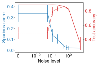
(a) Noisy input

(b) Weight decay

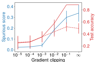
(c) Gradient clipping

Figure 8: Spurious score (solid blue line), clean test accuracy (solid red line), and spurious test accuracy (dotted red line) vs. the regularization strength on Fashion with different regularization methods. For the experiment, we fix the spurious pattern to be S3 and the target class $c_{tar}=0$. We compute the average spurious score and clean test accuracy across models trained with 1, 3, 5, 10, 20, and 100 spurious examples and five random seeds. The results for MNIST and CIFAR10 and spurious pattern R3 are in App. D, which shows similar results.

Results. The results are shown in Fig. 8. We see that with a properly set regularization strength for noisy input and weight decay, one may reduce the spurious score and increase spurious test accuracy without sacrificing much accuracy. This significantly reduces the undesirable consequences brought by rare spurious correlations. This aligns with our observation in the theoretical model and suggests that neural networks may share a similar property with linear models. We also find that gradient clipping cannot mitigate spurious correlation without reducing the test accuracy. Finally, we observe that all these methods are unable to completely avoid learning spurious correlations.

Data deletion methods. Another idea for mitigating rare spurious correlation is to apply data deletion methods (Izzo et al., 2021). In App. C, we experiment with two data deletion methods, incremental retraining and group influence functions (Basu et al., 2020a). However, they are not effective.

Discussion. Regarding mitigating rare spurious correlations, a provable way to prevent learning them is differential privacy (Dwork et al., 2006), which ensures that the participation of a single person (or a small group) in the dataset does not change the probability of any classifier by much. This requires noise addition during training, which may lead to a significant loss in accuracy (Chaudhuri et al., 2011; Abadi et al., 2016). If we know which are the spurious examples, then we can remove spurious correlations via an indistinguishable approximate data deletion method (Ginart et al., 2019; Neel et al., 2020); however, these methods provide lower accuracy for convex optimization and have no performance guarantees for non-convex. An open problem is to design algorithms or architectures that can mitigate these without sacrificing prediction accuracy.

Prior work (Sagawa et al., 2019; Kulynych et al., 2022) suggests that proper use of regularization methods plus well-designed loss functions can mitigate some types of spurious correlations. However, these regularization methods are used either in an ad-hoc manner or may reduce test accuracy. As shown in our experiment, not all regularization methods can remove rare spurious correlations without reducing the accuracy. This suggests that different regularization methods may be specifically tied to be able to mitigate certain kinds of spurious correlation. The exact role that regularization methods play in reducing spurious correlations is still an open question. Figuring out what kinds of spurious correlations can be mitigated by which regularization methods is an interesting future direction.

7 Related Work

Spurious correlations. Previous work has looked at spurious correlations in neural networks under various scenarios, including test time distribution shift (Sagawa et al., 2020; Srivastava et al., 2020; Bahng et al., 2020; Zhou et al., 2021; Khani & Liang, 2021), confounding factors in data collection  (Gururangan et al., 2018), the effect of image backgrounds (Xiao et al., 2020), and causality (Arjovsky et al., 2019). However, in most works, spurious examples often constitute a significant portion of the training set. In contrast, we look at spurious correlations introduced by a small number of examples (rare spurious correlations). Concurrent work (Hartley & Tsaftaris, 2022) measures spurious correlation caused by few examples. However, they did not show the consequences of these spurious correlations nor discuss ways to mitigate them.

Memorization in neural networks. Prior work has investigated how neural networks can inadvertently memorize training data (Arpit et al., 2017; Carlini et al., 2019; 2020; Feldman & Zhang, 2020; Leino & Fredrikson, 2020). Methods have also been proposed to measure this kind of memorization, including the use of the influence function (Feldman & Zhang, 2020) and likelihood estimates (Carlini et al., 2019). Our work focuses on partial memorization instead of memorizing individual examples, and our proposed method may be potentially applicable in more scenarios.

A line of work in the security literature exploits the memorization of certain patterns to compromise neural networks. The backdoor attack from Chen et al. (2017) attempts to change hard label predictions and accuracy by inserting carefully crafted spurious patterns. Sablayrolles et al. (2020) design specific markers that allow adversaries to detect whether images with those particular markers are used for training in a model. Another line of research on data poisoning attack Xiao et al. (2015); Wang & Chaudhuri (2018); Burkard & Lagesse (2017) aims to degrade the performance of a model by carefully altering the training data. In contrast, our work looks at rare spurious correlations from natural spurious patterns, instead of adversarially crafted ones. App. F has detailed discussions.

8 Conclusion

The learning of spurious correlation is a complex process, and it can have unintended consequences. As neural networks are getting more widely applied, it is crucial to better understand spurious correlations. There are many open questions remain. For example, besides the distribution shift that adds spurious features, are there any other types of distribution shift that will affect the accuracy? Another limitation of our current study is that our experiments are conducted only on image classification tasks, which may not generalize to others.

Acknowledgments

We thank Angel Hsing-Chi Hwang for providing thoughtful comments on the paper. This work was supported by NSF under CNS 1804829 and ARO MURI W911NF2110317. CNC’s research is supported by a Simons Investigator Fellowship, NSF grant DMS-2134157, DARPA grant W911NF2010021,and DOE grant DE-SC0022199.

The appendix is organized as follows.

• App. A: We provide a detailed analysis of our theoretical model.

• App. B: We show how different factors effects how rare spurious correlation is learned through different regularization methods, the norm of each pattern, network architectures, and the optimization algorithms.

• App. C: As removing the spurious examples should be able to remove the spurious correlations. The data deletion methods can be an intuitive approach to try. Here, we examine whether these methods are useful.

• App. D: We show the detailed experimental setup and present additional results here. The subsections include:

  • Sec. E.1 presents additional results of the qualitative study on how the weights of a neural network is effected by rare spurious correlations.

  • Sec. E.2 reports the spurious scores on MNIST, Fashion, and CIFAR10 when $c_{\text{tar}}=1$.

  • Sec. E.3 reports the membership inference results for MNIST, Fashion, and CIFAR10 with all spurious patterns.

  • Sec. E.4 reports results of additional experiments for the spurious test accuracy.

  • Sec. E.5 reports the results for additional spurious contexts.

  • Sec. E.6 presents an ablation study to see whether a normalized spurious score would effect the result.

• App. F: We present additional related work and discussions. The new contents include a detailed comparison with backdoor attacks, other methods for mitigating specific spurious correlations, short-cut learning, and simplicity bias.

Appendix A Details for Our Theoretical Model

In this section, we provide the details of our theoretical analysis in Sec. 5. To be self-contained, we review the mathematical language we use to discuss spurious correlations in Sec. A.1. Next, we provide the formal definitions of our training and testing models in Sec. A.2 and state the main results and implications in Sec. A.3. Finally, we give the complete proof for the main theorem in Sec. A.4

A.1 Preliminaries

Recall that we focus on the image classification task where $\mathcal{X}$ is an input space, and $\mathcal{Y}$ is a label space. An example is a pair $(\mathbf{x},y)\in\mathcal{X}\times\mathcal{Y}$ and at the training time, we are given a set of examples sampled from a distribution $\mathcal{D}_{\text{train}}$. At the testing time, we evaluate the network on either the clean test distribution $\mathcal{D}_{\text{ctest}}$ or the spurious test distribution $\mathcal{D}_{\text{stest}}$.

Spurious correlation. We model an input $\mathbf{x}$ as the output of a feature map $\Phi_{\mathcal{X}}$ from the feature space $\mathcal{X}_{\text{inv}}\times\mathcal{X}_{\text{sp}}$ to the input space $\mathcal{X}$ where $\mathcal{X}_{\text{inv}}$ is the invariant feature space containing the features that causally determine the label and $\mathcal{X}_{\text{sp}}$ is the spurious feature space that accommodates spurious features. $\Phi_{\mathcal{Y}}:\mathcal{X}_{\text{inv}}\to\mathcal{Y}$ is a function that maps the invariant feature $\mathbf{x}_{\text{inv}}$ to a label. Thus, an example $(\mathbf{x},y)$ is generated by $(\mathbf{x}_{\text{inv}},\mathbf{x}_{\text{sp}})$ via $\mathbf{x}=\Phi_{\mathcal{X}}(\mathbf{x}_{\text{inv}},\mathbf{x}_{\text{sp}})$ and $y=\Phi_{\mathcal{Y}}(\mathbf{x}_{\text{inv}})$. Without loss of generality, the zero vector in $\mathcal{X}_{\text{sp}}$, i.e., $0\in\mathcal{X}_{\text{sp}}$, refers to “no spurious feature” and for any nonzero $\mathbf{x}_{\text{sp}}$ we call $\Phi(\mathbf{x}_{\text{inv}},\mathbf{x}_{\text{sp}})-\Phi(\mathbf{x}_{\text{inv}},0)$ a spurious pattern. We focus on the case of having a fixed spurious feature $\mathbf{x}_{\text{sp}}$ and leave it as a future direction to study the more general scenarios where there are multiple spurious features.

Two simple models for spurious correlations. We consider two simple instantiations of $\Phi_{\mathcal{X}}$. First, the overlapping model (used in Sec. 3) where the spurious feature is put on top of the invariant feature, i.e., $\mathcal{X}=\mathcal{X}_{\text{inv}}=\mathcal{X}_{\text{sp}}$ and $\Phi_{\mathcal{X}}(\mathbf{x}_{\text{inv}},\mathbf{x}_{\text{sp}})=\mathbf{x}_{\text{inv}}+\mathbf{x}_{\text{sp}}$ or $\Phi_{\mathcal{X}}(\mathbf{x}_{\text{inv}},\mathbf{x}_{\text{sp}})=clip(\mathbf{x}_{\text{inv}}+\mathbf{x}_{\text{sp}})$ where $clip$ is a function that truncates an input pixel when its value exceeds a certain range. Second, the concatenate model (used in Sec. 5) where the spurious feature is concatenated to the invariant feature, i.e., $\mathcal{X}=\mathcal{X}_{\text{inv}}\times\mathcal{X}_{\text{sp}}$ and $\Phi_{\mathcal{X}}(\mathbf{x}_{\text{inv}},\mathbf{x}_{\text{sp}})=(\mathbf{x}_{\text{inv}},\mathbf{x}_{\text{sp}})$.

A.2 Our training and testing models

Here we delineate the theoretical model described in Sec. 5.1. Recall that we consider a binary classification task to model where $\mathcal{X}=\mathcal{X}_{\text{inv}}\times\mathcal{X}_{\text{sp}}$ is an input vector space and $\mathcal{Y}=\{-1,1\}$ is a label space. $\gamma\in[0,1]$ is the parameter for the fraction of spurious samples and in this paper we focus on the regime where $\gamma$ is very close to $0$. $\mathbf{x}_{-},\mathbf{x}_{+}\in\mathcal{X}_{\text{inv}}$ are the invariant features of the two classes and after a linear shift we can without loss of generality have $\mathbf{x}_{-}=-\mathbf{x}_{+}$. Let $\mathbf{x}_{\text{sp}}\in\mathcal{X}_{\text{sp}}$ be the spurious feature where we call its length, $\|\mathbf{x}_{\text{sp}}\|_{2}$, the spurious signal strength. Finally, $\sigma_{\text{inv}}^{2},\sigma_{\text{sp}}^{2}>0$ are the parameters for the variance along $\mathcal{X}_{\text{inv}}$ and $\mathcal{X}_{\text{sp}}$ respectively. Now, we formally define the training distribution $\mathcal{D}_{\text{train}}=\mathcal{D}_{\text{train}}(\gamma,\mathbf{x}_{-},\mathbf{x}_{+},\mathbf{x}_{\text{sp}},\sigma_{\text{inv}},\sigma_{\text{sp}})$, the clean text distribution $\mathcal{D}_{\text{ctest}}=\mathcal{D}_{\text{ctest}}(\gamma,\mathbf{x}_{-},\mathbf{x}_{+},\mathbf{x}_{\text{sp}},\sigma_{\text{inv}},\sigma_{\text{sp}})$, and the spurious test distribution $\mathcal{D}_{\text{stest}}=\mathcal{D}_{\text{ctest}}(\gamma,\mathbf{x}_{-},\mathbf{x}_{+},\mathbf{x}_{\text{sp}},\sigma_{\text{inv}},\sigma_{\text{sp}})$ as follows.

Definition 1.

Let $\Sigma:=\sigma_{\text{inv}}^{2}I_{\text{inv}}+\sigma_{\text{sp}}^{2}I_{\text{sp}}$ where $I_{\text{inv}}$ and $I_{\text{sp}}$ are identity matrix for $\mathcal{X}_{\text{inv}}$ and $\mathcal{X}_{\text{sp}}$ respectively.

• $\mathcal{D}_{\text{train}}(\gamma,\mathbf{x}_{-},\mathbf{x}_{+},\mathbf{x}_{\text{sp}},\sigma_{\text{inv}},\sigma_{\text{sp}})$ samples $(\mathbf{x},y)$ using the following process:

  • with probability $1/2$, $\mathbf{x}\sim\mathcal{N}((\mathbf{x}_{-},0),\Sigma)$ and $y=-1$;

  • with probability $(1-\gamma)/2$, $\mathbf{x}\sim\mathcal{N}((\mathbf{x}_{+},0),\Sigma)$ and $y=+1$;

  • with probability $\gamma/2$, $\mathbf{x}\sim\mathcal{N}((\mathbf{x}_{+},\mathbf{x}_{\text{sp}}),\Sigma)$ and $y=+1$.

• $\mathcal{D}_{\text{ctest}}(\gamma,\mathbf{x}_{-},\mathbf{x}_{+},\mathbf{x}_{\text{sp}},\sigma_{\text{inv}},\sigma_{\text{sp}})$ samples $(\mathbf{x},y)$ using the following process:

  • with probability $1/2$, $\mathbf{x}\sim\mathcal{N}((\mathbf{x}_{-},0),\Sigma)$ and $y=-1$;

  • with probability $1/2$, $\mathbf{x}\sim\mathcal{N}((\mathbf{x}_{+},0),\Sigma)$ and $y=+1$.

• $\mathcal{D}_{\text{stest}}(\gamma,\mathbf{x}_{-},\mathbf{x}_{+},\mathbf{x}_{\text{sp}},\sigma_{\text{inv}},\sigma_{\text{sp}})$ samples $(\mathbf{x},y)$ with $\mathbf{x}\sim\mathcal{N}((\mathbf{x}_{-},\mathbf{x}_{\text{sp}}),\Sigma)$ and $y=-1$.

Now, we can instantiate our model into examples that capture the experimental scenarios discussed in previous sections (see Fig. 1). For examples, the patterns small 1 (S1), small 2 (S2), and small 3 (S3) correspond to setting $\sigma_{\text{sp}}=0$ and increasing the strength of spurious features (i.e., increasing $\|\mathbf{x}_{\text{sp}}\|_{2}$ from (S1) to (S3)). Also, see Fig. 9 for a pictorial explanation of our model.

(a) $\mathcal{D}_{\text{train}},\gamma=0$.

(b) $\mathcal{D}_{\text{train}},\gamma>0$.

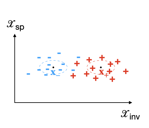
(c) $\mathcal{D}_{\text{ctest}}$.

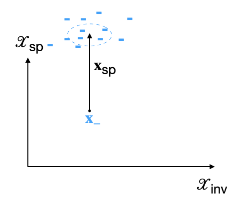
(d) $\mathcal{D}_{\text{stest}}$.

Figure 9: Examples of the training distribution $\mathcal{D}_{\text{train}}$ and phase transitions in our theoretical model. (a)-(b) With equal probability a training example is sampled from either $\mathcal{N}(\mathbf{x}_{+},\sigma_{\text{inv}}I_{\text{inv}}+\sigma_{\text{sp}}I_{\text{sp}})$ or $\mathcal{N}(\mathbf{x}_{-},\sigma_{\text{inv}}I_{\text{inv}}+\sigma_{\text{sp}}I_{\text{sp}})$. With probability $\gamma$, a $+$ sample will be concatenated with the spurious pattern $\mathbf{x}_{\text{sp}}$. The dotted line is the decision boundary of the optimal classifier. (c) The clean test distribution $\mathcal{D}_{\text{ctest}}$, which is the same as $\mathcal{D}_{\text{train}}$ with $\gamma=0$. (d) The spurious test distribution $\mathcal{D}_{\text{stest}}$, which only contains $-$ samples with spurious pattern $\mathbf{x}_{\text{sp}}$ added.

A.3 Analysis for linear regression with mean square loss and $\ell_{2}$ regularization

As the theoretical toolkit for understanding neural networks is far from complete, we examine the theoretical aspect of rare spurious correlations through the lens of a classic learning algorithm: linear regression with mean square loss. Notice that we do not claim that the analysis here generalize to neural networks. Instead, the analysis for linear regression serves as food for thoughts for future investigation.

For linear regression with mean square loss, the hypothesis set is $\mathbb{H}=\{h=(\bm{\beta}_{\text{inv}},\bm{\beta}_{\text{sp}},\beta_{0}):\bm{\beta}_{\text{inv}}\in\mathcal{X}_{\text{inv}},\bm{\beta}_{\text{sp}}\in\mathcal{X}_{\text{sp}},\beta_{0}\in\mathbb{R}\}$ where $h(\mathbf{x})=\bm{\beta}_{\text{inv}}^{\top}\mathbf{x}_{\text{inv}}+\bm{\beta}_{\text{sp}}^{\top}\mathbf{x}_{\text{sp}}+\beta_{0}$. The $\ell_{2}$ loss function of $h$ on a distribution $\mathcal{D}$ is denotes as $L_{\mathcal{D}}(h):=\frac{1}{2}\mathbb{E}_{(\mathbf{x},y)\sim\mathcal{D}}[(h(\mathbf{x})\cdot y-1)^{2}]$. If we consider adding $\ell_{2}$ regularization with parameter $\lambda$, the loss function becomes $L_{\mathcal{D}}(h):=\frac{1}{2}\mathbb{E}_{(\mathbf{x},y)\sim\mathcal{D}}[(h(\mathbf{x})\cdot y-1)^{2}]+\frac{\lambda}{2}\|\bm{\beta}_{\text{inv}}\|_{2}^{2}+\frac{\lambda}{2}\|\bm{\beta}_{\text{sp}}\|_{2}^{2}$. In the rest of this section, we focus on the setting with $\ell_{2}$ regularization since the unregularized setting can be obtained by setting $\lambda=0$.

The optimal classifier in $\mathbb{H}$ for $\mathcal{D}_{\text{train}}$ is defined to be $h^{*}:=\arg\min_{h\in\mathbb{H}}L_{\mathcal{D}_{\text{train}}}(h)$. By the theory of linear regression with mean square loss, we know that $h^{*}$ can be found via standard Empirical Risk Minimization (ERM) principle. In our theoretical analysis, we study the performance of $h^{*}$ while one can easily extend our analysis to the finite sample regime by applying the standard convergence analysis of ERM for linear regression with mean square loss.

There are three quantities of interest in our study of rare spurious correlations: clean test accuracy, spurious test accuracy, and spurious score. For the completeness of presentation, let us formally define them as follows.

Definition 2 (Test accuracy).

Let $h$ be a hypothesis function and $\mathcal{D}_{\text{test}}$ be a test distribution. The test accuracy of $h$ on $\mathcal{D}_{\text{test}}$ is defined as

$$Acc_{\mathcal{D}_{\text{test}}}(h):=\Pr_{(\mathbf{x},y)\sim\mathcal{D}_{\text{test}}}[h(\mathbf{x})y>0]\,.$$

Definition 3 (Prediction difference and Spurious score).

Let $h$ be a hypothesis function, $\mathcal{D}_{\text{test}}$ be a test distribution, $(\Phi_{\mathcal{X}},\Phi_{\mathcal{Y}})$ be the feature-to-input maps, and $\mathbf{x}_{\text{sp}}$ be a spurious feature. The prediction difference for an invariant input $\mathbf{x}\in\mathcal{X}_{\text{inv}}$ is defined as

$$PD(\mathbf{x};h):=h(\Phi_{\mathcal{X}}(\mathbf{x},\mathbf{x}_{\text{sp}}))-h(\Phi_{\mathcal{X}}(\mathbf{x},0))\,.$$

For every $\epsilon>0$, the $\epsilon$-spurious score of $h$ with respect to $\mathcal{D}_{\text{test}}$ is defined as

$$\epsilon\text{-spurious-score}(h)=\Pr_{(\mathbf{x},y)\sim\mathcal{D}_{\text{test}}}[PD(\mathbf{x},h)>\epsilon]\,.$$

Note that for linear classifier in both the overlap and the concatenation model, the $\epsilon$-spurious-score is always either $0$ or $1$ because $PD(\mathbf{x};h)=h(\mathbf{x}_{\text{sp}})$ for every $\mathbf{x}\in\mathcal{X}_{\text{inv}}$. Thus, for a linear classifier $h$, we denote $PD(h)=h(\mathbf{x}_{\text{sp}})$ for simplicity. In the rest of the theoretical analysis, we study the prediction difference which tells us when does the spurious score jump from $0$ to $1$.

Now, we state our main theorem about the clean test accuracy, spurious test accuracy, and the prediction difference of $h^{*}$. We remark that the calculations for these quantities are straightforward and we postpone the proof to Sec. A.4.

Theorem 1.

For every $\gamma\in(0,1]$, $\lambda>0$, $\mathbf{x}_{\text{inv}}\in\mathcal{X}_{\text{inv}}$, $\mathbf{x}_{\text{sp}}\in\mathcal{X}_{\text{sp}}$, and $\sigma_{\text{inv}}^{2},\sigma_{\text{sp}}^{2}>0$. Let $h^{*}$ be the optimal classifier for $\mathcal{D}_{\text{train}}=\mathcal{D}_{\text{train}}(\gamma,-\mathbf{x}_{\text{inv}},\mathbf{x}_{\text{inv}},\mathbf{x}_{\text{sp}},\sigma_{\text{inv}}^{2},\sigma_{\text{sp}}^{2})$ using linear regression with mean square loss and $\ell_{2}$ regularization with parameter $\lambda$. We have

$$Acc_{\mathcal{D}_{\text{ctest}}}(h^{*}) =\frac{1}{2}\Phi\left(\frac{\frac{\frac{\gamma}{2}(1-\gamma)\|\mathbf{x}_{\text{sp}}\|_{2}^{2}+\sigma_{\text{sp}}^{2}+\lambda}{\sigma_{\text{inv}}^{2}+\lambda}\|\mathbf{x}_{\text{inv}}\|_{2}^{2}+(\frac{\gamma}{2})^{2}\|\mathbf{x}_{\text{sp}}\|_{2}^{2}}{\sqrt{\left(\frac{\frac{\gamma}{2}(1-\gamma)\|\mathbf{x}_{\text{sp}}\|_{2}^{2}+\sigma_{\text{sp}}^{2}+\lambda}{\sigma_{\text{inv}}^{2}+\lambda}\right)^{2}\|\mathbf{x}_{\text{inv}}\|_{2}^{4}\sigma_{\text{inv}}^{2}+(\frac{\gamma}{2})^{2}\|\mathbf{x}_{\text{sp}}\|_{2}^{4}\sigma_{\text{sp}}^{2}}}\right)$$

$$+\frac{1}{2}\Phi\left(\frac{\frac{\frac{\gamma}{2}(1-\gamma)\|\mathbf{x}_{\text{sp}}\|_{2}^{2}+\sigma_{\text{sp}}^{2}+\lambda}{\sigma_{\text{inv}}^{2}+\lambda}\|\mathbf{x}_{\text{inv}}\|_{2}^{2}-(\frac{\gamma}{2})^{2}\|\mathbf{x}_{\text{sp}}\|_{2}^{2}}{\sqrt{\left(\frac{\frac{\gamma}{2}(1-\gamma)\|\mathbf{x}_{\text{sp}}\|_{2}^{2}+\sigma_{\text{sp}}^{2}+\lambda}{\sigma_{\text{inv}}^{2}+\lambda}\right)^{2}\|\mathbf{x}_{\text{inv}}\|_{2}^{4}\sigma_{\text{inv}}^{2}+(\frac{\gamma}{2})^{2}\|\mathbf{x}_{\text{sp}}\|_{2}^{4}\sigma_{\text{sp}}^{2}}}\right)$$

and

$$Acc_{\mathcal{D}_{\text{stest}}}(h^{*})=\Phi\left(\frac{\frac{\frac{\gamma}{2}(1-\gamma)\|\mathbf{x}_{\text{sp}}\|_{2}^{2}+\sigma_{\text{sp}}^{2}+\lambda}{\sigma_{\text{inv}}^{2}+\lambda}\|\mathbf{x}_{\text{inv}}\|_{2}^{2}+(\frac{\gamma}{2}-1)\frac{\gamma}{2}\|\mathbf{x}_{\text{sp}}\|_{2}^{2}}{\sqrt{\left(\frac{\frac{\gamma}{2}(1-\gamma)\|\mathbf{x}_{\text{sp}}\|_{2}^{2}+\sigma_{\text{sp}}^{2}+\lambda}{\sigma_{\text{inv}}^{2}+\lambda}\right)^{2}\|\mathbf{x}_{\text{inv}}\|_{2}^{4}\sigma_{\text{inv}}^{2}+(\frac{\gamma}{2})^{2}\|\mathbf{x}_{\text{sp}}\|_{2}^{4}\sigma_{\text{sp}}^{2}}}\right)$$

and

$$PD(h^{*})=\frac{\frac{\gamma}{2}(\sigma_{\text{inv}}^{2}+\lambda)\|\mathbf{x}_{\text{sp}}\|_{2}^{2}}{(\sigma_{\text{inv}}^{2}+\lambda)(\sigma_{\text{sp}}^{2}+\lambda)+\left(\sigma_{\text{sp}}^{2}+\lambda+\frac{\gamma}{2}(1-\frac{\gamma}{2})(\sigma_{\text{inv}}^{2}+\lambda)+\frac{\gamma}{2}(1-\gamma)\|\mathbf{x}_{\text{sp}}\|_{2}^{2}\right)\|\mathbf{x}_{\text{sp}}\|_{2}^{2}}$$

where $\Phi(\cdot)$ is the cumulative distribution function (CDF) of the standard Gaussian variable.

A.3.1 Implications of Theorem 1

In Sec. 5.2 we present three observations given by Theorem 1 without explaining why. Here, we provide all the underlying reasoning.

Observation 1: A phase transition of spurious test accuracy and prediction difference at $\gamma=0$. Note that by Theorem 1, when $\gamma$ is close to $0$, the spurious test accuracy and the prediction difference is approximately

$$ACC_{\mathcal{D}_{\text{stest}}}=\Phi\left(1-\frac{(\sigma_{\text{inv}}^{2}+\lambda)\|\mathbf{x}_{\text{sp}}\|_{2}^{2}}{2(\sigma_{\text{sp}}^{2}+\lambda)\|\mathbf{x}_{\text{inv}}\|_{2}^{2}\sigma_{\text{inv}}}\gamma\right)$$

and

$$PD(h^{*})=\frac{(\sigma_{\text{inv}}^{2}+\lambda)\|\mathbf{x}_{\text{sp}}\|_{2}^{2}}{2(\sigma_{\text{sp}}^{2}+\lambda)(\sigma_{\text{inv}}^{2}+\lambda+\|\mathbf{x}_{\text{sp}}\|_{2}^{2})}\gamma\,.$$

One can see that when $\|\mathbf{x}_{\text{sp}}\|_{2}^{2}/\sigma_{\text{sp}}^{2}$ is large, the spurious test accuracy (resp. prediction difference) undergoes a sharp decay (resp. growth) within an interval near $\gamma=0$. In particular, the sharp decay/growth ends at $\gamma\approx\Theta(\min\{1,\frac{\sigma_{\text{sp}}^{2}+\lambda}{\|\mathbf{x}_{\text{sp}}\|_{2}^{2}},\frac{\sigma_{\text{sp}}^{2}+\lambda}{\sigma_{\text{sp}}\|\mathbf{x}_{\text{sp}}\|_{2}^{2}(\sigma_{\text{inv}}^{2}+\lambda)}\})$. As it is analytically hard to get a precise characterization of the critical point, we also numerically plot the spurious test accuracy and the prediction difference under different parameters to demonstrate the phase transition phenomenon.

Observation 2: adding Gaussian noises lowers spurious score. Note that adding (isotropic) Gaussian noises with strength $\sigma^{2}$ to input $\mathbf{x}$ is equivalent to increase the variance by an additive factor of $\sigma^{2}$, i.e., $\sigma_{\text{inv}}^{2}\leftarrow\sigma_{\text{inv}}^{2}+\sigma^{2}$ and $\sigma_{\text{sp}}^{2}\leftarrow\sigma_{\text{sp}}^{2}+\sigma^{2}$. Empirically we observe in Fig. 10 that both the clean test accuracy and spurious test accuracy decay as $\sigma^{2}$ becomes larger while the prediction difference decays favorably. Intuitively, adding Gaussian noises decrease the signal-to-noise ratio of both the invariant feature and the spurious feature.

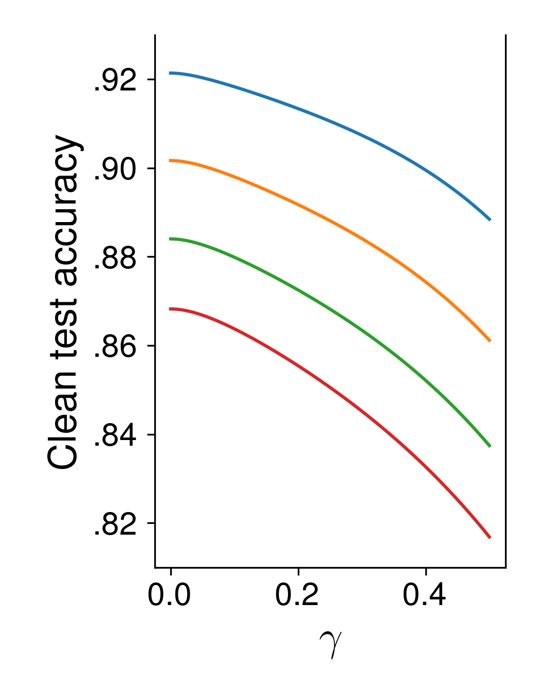
(a) ctest SNR $\downarrow$

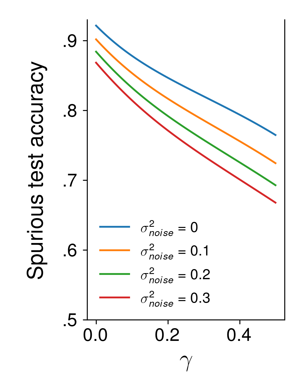
(b) stest SNR $\downarrow$

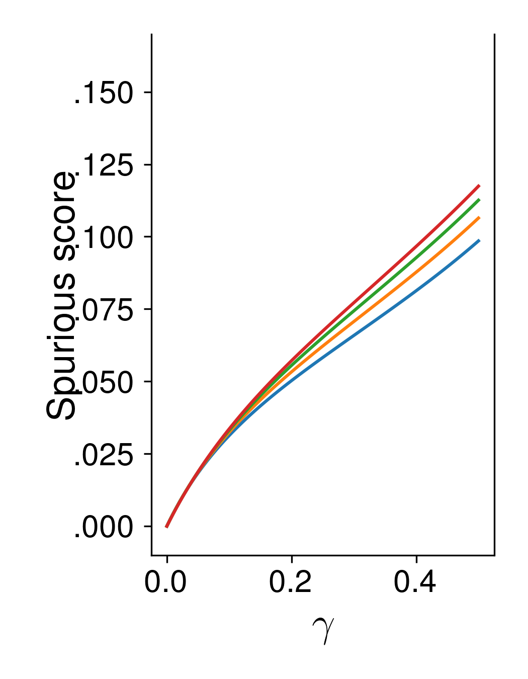
(c) sscore SNR $\downarrow$

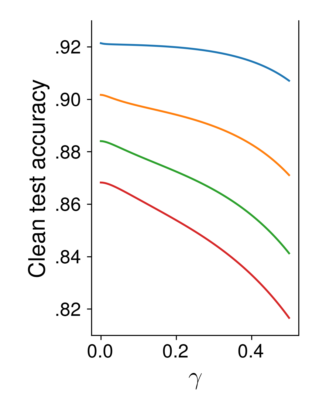
(d) ctest SNR $\uparrow$

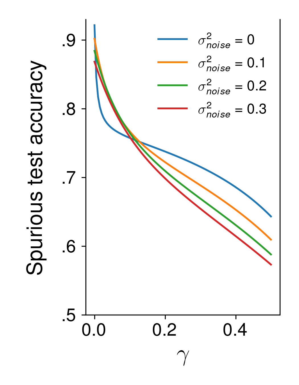
(e) stest SNR $\uparrow$

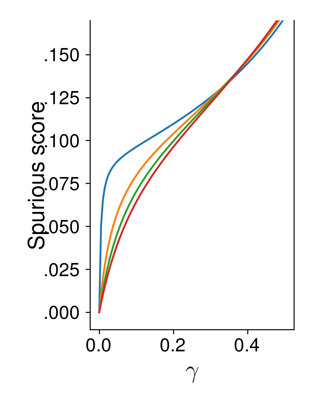
(f) sscore SNR $\uparrow$

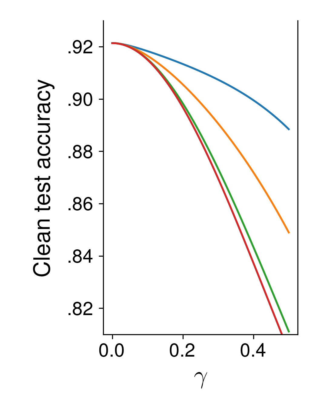
(g) ctest SNR $\downarrow$

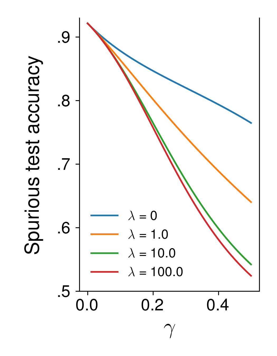
(h) stest SNR $\downarrow$

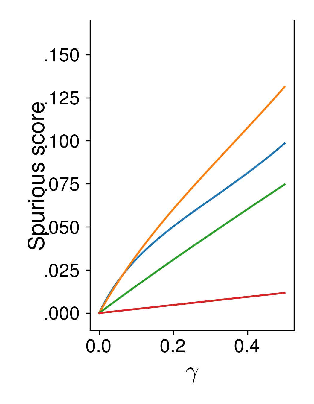
(i) sscore SNR $\downarrow$

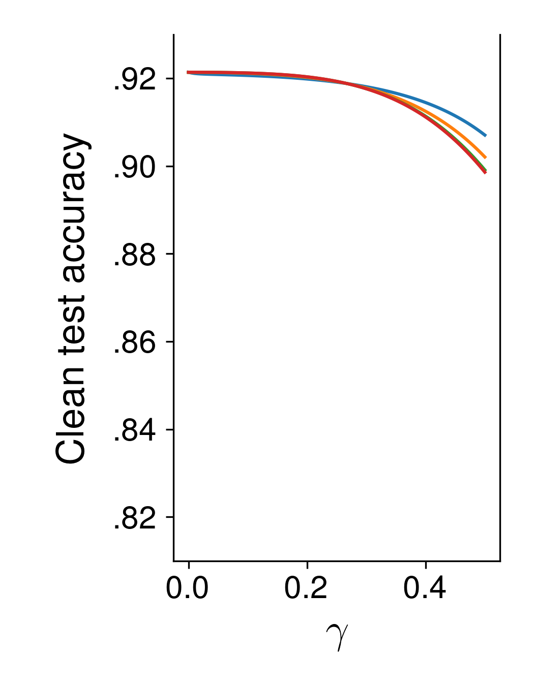
(j) ctest SNR $\uparrow$

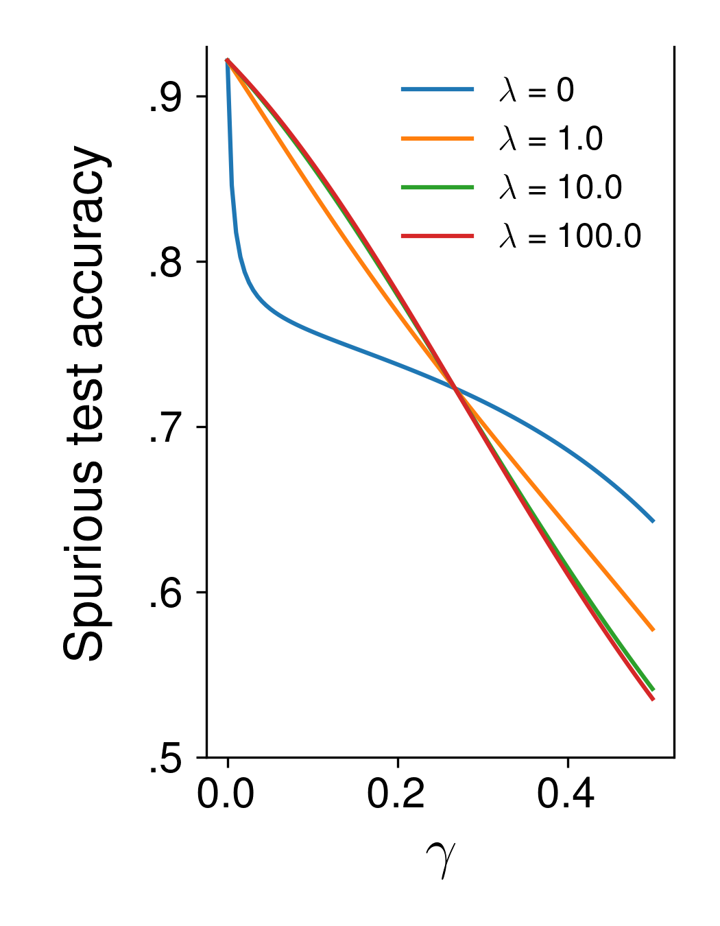
(k) stest SNR $\uparrow$

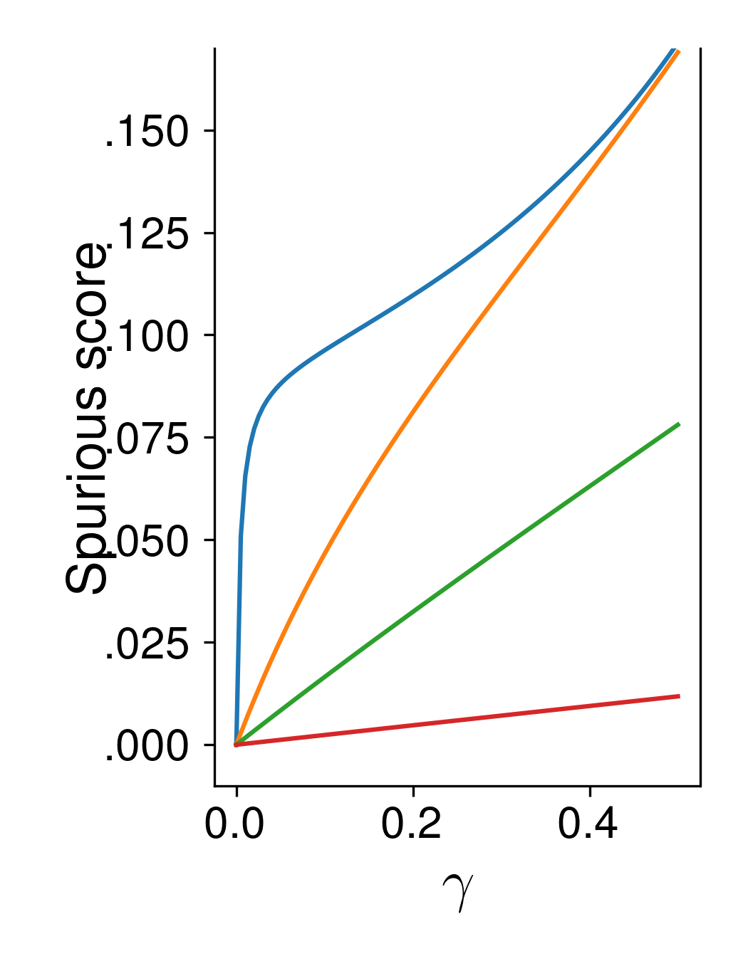
(l) sscore SNR $\uparrow$

Figure 10: Examples of the effect of adding Gaussian noises and $\ell_{2}$ regularization under different regime of signal-to-noise ratio (SNR) $\|\mathbf{x}_{\text{sp}}\|_{2}/\sigma_{\text{sp}}^{2}$. For low SNR, we have $\|\mathbf{x}_{\text{sp}}\|_{2}/\sigma_{\text{sp}}^{2}=10$, and for high SNR, we have $\|\mathbf{x}_{\text{sp}}\|_{2}/\sigma_{\text{sp}}^{2}=1=500$. (a)-(f) show the effect of adding different strength of Gaussian noises and (g)-(l) show the effect of different $\ell_{2}$ regularization strength. Here, we shorthand clean test accuracy as ctest, spurious test accuracy as stest and spurious score as sscore.

Observation 3: $\ell_{2}$ regularization improves test accuracy and lowers spurious score. The main difference of $\ell_{2}$ regularization from adding Gaussian noises is that it non-uniformly increasing the effective variance of the invariant subspace and that of the spurious subspace. This can be seen from the formulas in Theorem 1 that the regularization parameter $\lambda$ is only added to some but not all of the $\sigma_{\text{inv}}^{2}$ and $\sigma_{\text{sp}}^{2}$. Numerically, we also plot the test accuracy and the prediction difference under different parameters to demonstrate the effect of $\ell_{2}$ regularization in Fig. 10.

A.4 Proof of Theorem 1

Proof.

For notational simplicity, in this proof we will overload the notations $\mathbf{x}_{\text{inv}}=(\mathbf{x}_{\text{inv}},0)\in\mathcal{X}$, $\mathbf{x}_{\text{sp}}=(0,\mathbf{x}_{\text{sp}})\in\mathcal{X}$, $\mathbf{x}_{\text{inv}}=(\mathbf{x}_{\text{inv}},0)\in\mathcal{X}$ and $-\mathbf{x}_{\text{inv}}=(-\mathbf{x}_{\text{inv}},0)\in\mathcal{X}$. Also, we denote $\beta=(\bm{\beta}_{\text{inv}},\bm{\beta}_{\text{sp}})$.

Let us start with finding $h^{*}$ via explicitly calculating the derivatives of loss function under $\mathcal{D}_{\text{train}}$ as follows.

Claim 1.

For every $h=(\bm{\beta}_{\text{inv}},\bm{\beta}_{\text{sp}},\beta_{0})\in\mathbb{H}$, we have

$$\frac{\partial}{\partial\beta}L_{\mathcal{D}_{\text{train}}}(h) =(\sigma_{\text{inv}}^{2}+\lambda)\bm{\beta}_{\text{inv}}+\left(\mathbf{x}_{\text{inv}}^{\top}\bm{\beta}_{\text{inv}}+\frac{\gamma\mathbf{x}_{\text{sp}}^{\top}\bm{\beta}_{\text{sp}}}{2}-1\right)\mathbf{x}_{\text{inv}}$$

$$+(\sigma_{\text{sp}}^{2}+\lambda)\bm{\beta}_{\text{sp}}+\frac{\gamma}{2}\left(\mathbf{x}_{\text{inv}}^{\top}\bm{\beta}_{\text{inv}}+\mathbf{x}_{\text{sp}}^{\top}\bm{\beta}_{\text{sp}}+\beta_{0}-1\right)\mathbf{x}_{\text{sp}}\,,$$

$$\frac{\partial}{\partial\beta_{0}}L_{\mathcal{D}_{\text{train}}}(h) =\frac{\gamma\mathbf{x}_{\text{sp}}^{\top}\bm{\beta}_{\text{sp}}}{2}+\beta_{0}\,.$$

The proof of Claim 1 follows from a direct calculation and we postpone the details to Section A.4.1.

As the loss function is a quadratic function, it suffices to solve the equations $\frac{\partial}{\partial\beta}L_{\mathcal{D}_{\text{train}}}(h)=0$ and $\frac{\partial}{\partial\beta_{0}}L_{\mathcal{D}_{\text{train}}}(h)=0$. Note that since the invariant subspace $\mathcal{X}_{\text{inv}}$ is orthogonal to the spurious subspace $\mathcal{X}_{\text{sp}}$, this enforces $\bm{\beta}_{\text{inv}}$ (resp. $\bm{\beta}_{\text{sp}}$) to be a scalar multiplication of $\mathbf{x}_{\text{inv}}$ (resp. $\mathbf{x}_{\text{sp}}$). Let us set $\bm{\beta}_{\text{inv}}=a\mathbf{x}_{\text{inv}}$ and $\bm{\beta}_{\text{sp}}=b\mathbf{x}_{\text{sp}}$ and solve $a,b$ by setting the partial derivatives to be zero. Namely, we get the following equations.

$$0 =a(\sigma_{\text{inv}}^{2}+\lambda)+a\|\mathbf{x}_{\text{inv}}\|_{2}^{2}+\frac{\gamma\|\mathbf{x}_{\text{sp}}\|_{2}^{2}}{2}b-1\,,$$

$$0 =b(\sigma_{\text{sp}}^{2}+\lambda)+\frac{\gamma}{2}(a\|\mathbf{x}_{\text{inv}}\|_{2}^{2}+b\|\mathbf{x}_{\text{sp}}\|_{2}^{2}+\beta_{0}-1)\,,$$

$$0 =\frac{\gamma\|\mathbf{x}_{\text{sp}}\|_{2}^{2}}{2}b+\beta_{0}\,.$$

By solving the above system of linear equations, we get

$$b =\frac{\frac{\gamma}{2}(\sigma_{\text{inv}}^{2}+\lambda)}{(\sigma_{\text{inv}}^{2}+\lambda)(\sigma_{\text{sp}}^{2}+\lambda)+\left(\sigma_{\text{sp}}^{2}+\lambda+\frac{\gamma}{2}(1-\frac{\gamma}{2})(\sigma_{\text{inv}}^{2}+\lambda)+\frac{\gamma}{2}(1-\gamma)\|\mathbf{x}_{\text{sp}}\|_{2}^{2}\right)\|\mathbf{x}_{\text{sp}}\|_{2}^{2}}\,,$$ (2)

$$\frac{a}{b} =\frac{\frac{\gamma}{2}(1-\gamma)\|\mathbf{x}_{\text{sp}}\|_{2}^{2}+\sigma_{\text{sp}}^{2}+\lambda}{\frac{\gamma}{2}(\sigma_{\text{inv}}^{2}+\lambda)}\,,$$ (3)

$$\frac{\beta_{0}}{b} =-\frac{\gamma\|\mathbf{x}_{\text{sp}}\|_{2}^{2}}{2}\,.$$ (4)

Now that we know what $h^{*}$ is, we can calculate the clean test accuracy as follows.

$$ACC_{\mathcal{D}_{\text{ctest}}}(h^{*}) =\Pr_{(\mathbf{x},y)\sim\mathcal{D}_{\text{ctest}}}[h^{*}(\mathbf{x})y>0]$$

$$=\frac{1}{2}\Pr_{\mathbf{x}\sim\mathcal{N}((-\mathbf{x}_{\text{inv}},0),\Sigma)}[h^{*}(\mathbf{x})<0]+\frac{1}{2}\Pr_{\mathbf{x}\sim\mathcal{N}((\mathbf{x}_{\text{inv}},0),\Sigma)}[h^{*}(\mathbf{x})>0]$$

$$=\frac{1}{2}\Pr_{\mathbf{w}\sim\mathcal{N}(0,\Sigma)}[\beta^{\top}(\mathbf{w}-\mathbf{x}_{\text{inv}})+\beta_{0}<0]+\frac{1}{2}\Pr_{\mathbf{w}\sim\mathcal{N}(0,\Sigma)}[\beta^{\top}(\mathbf{w}+\mathbf{x}_{\text{inv}})+\beta_{0}>0]\,.$$

As $$\mathcal{N}(0,\Sigma) \mathcal{X}_{\text{inv}} \mathcal{X}_{\text{sp}}$$ is isotropic in both and , the above becomes

$$=\frac{1}{2}\Pr_{\mathbf{w}\sim\mathcal{N}(0,\Sigma)}[\beta^{\top}(\mathbf{w}-\mathbf{x}_{\text{inv}})<-\beta_{0}]+\frac{1}{2}\Pr_{\mathbf{w}\sim\mathcal{N}(0,\Sigma)}[\beta^{\top}(\mathbf{w}-\mathbf{x}_{\text{inv}})<\beta_{0}]$$

$$=\frac{1}{2}\Pr_{\begin{subarray}{c}\mathbf{w}_{\text{inv}}\sim\mathcal{N}(0,\sigma_{\text{inv}}^{2}I_{\text{inv}})\\ \mathbf{w}_{\text{sp}}\sim\mathcal{N}(0,\sigma_{\text{sp}}^{2}I_{\text{sp}})\end{subarray}}[a\mathbf{x}_{\text{inv}}^{\top}\mathbf{w}_{\text{inv}}+b\mathbf{x}_{\text{sp}}^{\top}\mathbf{w}_{\text{sp}}<a\|\mathbf{x}_{\text{inv}}\|_{2}^{2}-\beta_{0}]$$

$$+\frac{1}{2}\Pr_{\begin{subarray}{c}\mathbf{w}_{\text{inv}}\sim\mathcal{N}(0,\sigma_{\text{inv}}^{2}I_{\text{inv}})\\ \mathbf{w}_{\text{sp}}\sim\mathcal{N}(0,\sigma_{\text{sp}}^{2}I_{\text{sp}})\end{subarray}}[a\mathbf{x}_{\text{inv}}^{\top}\mathbf{w}_{\text{inv}}+b\mathbf{x}_{\text{sp}}^{\top}\mathbf{w}_{\text{sp}}<a\|\mathbf{x}_{\text{inv}}\|_{2}^{2}+\beta_{0}]\,.$$

Note that $$a\mathbf{x}_{\text{inv}}^{\top}\mathbf{w}_{\text{inv}}+b\mathbf{x}_{\text{sp}}^{\top}\mathbf{w}_{\text{sp}} \mathcal{N}(0,\sigma^{2}) \sigma^{2}=a^{2}\|\mathbf{x}_{\text{inv}}\|_{2}^{4}\sigma_{\text{inv}}^{2}+b^{2}\|\mathbf{x}_{\text{sp}}\|_{2}^{4}\sigma_{\text{sp}}^{2}$$ follows the distribution where . Namely, the above can be further simplified as

$$=\frac{1}{2}\Pr_{w\sim\mathcal{N}(0,\sigma^{2})}[w<a\|\mathbf{x}_{\text{inv}}\|_{2}^{2}+\beta_{0}]+\frac{1}{2}\Pr_{w\sim\mathcal{N}(0,\sigma^{2})}[w<a\|\mathbf{x}_{\text{inv}}\|_{2}^{2}-\beta_{0}]$$

$$=\frac{1}{2}\Phi\left(\frac{a\|\mathbf{x}_{\text{inv}}\|_{2}^{2}-\beta_{0}}{\sqrt{a^{2}\|\mathbf{x}_{\text{inv}}\|_{2}^{4}\sigma_{\text{inv}}^{2}+b^{2}\|\mathbf{x}_{\text{sp}}\|_{2}^{4}\sigma_{\text{sp}}^{2}}}\right)+\frac{1}{2}\Phi\left(\frac{a\|\mathbf{x}_{\text{inv}}\|_{2}^{2}+\beta_{0}}{\sqrt{a^{2}\|\mathbf{x}_{\text{inv}}\|_{2}^{4}\sigma_{\text{inv}}^{2}+b^{2}\|\mathbf{x}_{\text{sp}}\|_{2}^{4}\sigma_{\text{sp}}^{2}}}\right)\,.$$

Lastly, by plugging in Eqs. 2, 3 and 4, the clean test accuracy of $$h^{*}$$ is

$$=\frac{1}{2}\Phi\left(\frac{\frac{\frac{\gamma}{2}(1-\gamma)\|\mathbf{x}_{\text{sp}}\|_{2}^{2}+\sigma_{\text{sp}}^{2}+\lambda}{\sigma_{\text{inv}}^{2}+\lambda}\|\mathbf{x}_{\text{inv}}\|_{2}^{2}+(\frac{\gamma}{2})^{2}\|\mathbf{x}_{\text{sp}}\|_{2}^{2}}{\sqrt{\left(\frac{\frac{\gamma}{2}(1-\gamma)\|\mathbf{x}_{\text{sp}}\|_{2}^{2}+\sigma_{\text{sp}}^{2}+\lambda}{\sigma_{\text{inv}}^{2}+\lambda}\right)^{2}\|\mathbf{x}_{\text{inv}}\|_{2}^{4}\sigma_{\text{inv}}^{2}+(\frac{\gamma}{2})^{2}\|\mathbf{x}_{\text{sp}}\|_{2}^{4}\sigma_{\text{sp}}^{2}}}\right)$$

$$+\frac{1}{2}\Phi\left(\frac{\frac{\frac{\gamma}{2}(1-\gamma)\|\mathbf{x}_{\text{sp}}\|_{2}^{2}+\sigma_{\text{sp}}^{2}+\lambda}{\sigma_{\text{inv}}^{2}+\lambda}\|\mathbf{x}_{\text{inv}}\|_{2}^{2}-(\frac{\gamma}{2})^{2}\|\mathbf{x}_{\text{sp}}\|_{2}^{2}}{\sqrt{\left(\frac{\frac{\gamma}{2}(1-\gamma)\|\mathbf{x}_{\text{sp}}\|_{2}^{2}+\sigma_{\text{sp}}^{2}+\lambda}{\sigma_{\text{inv}}^{2}+\lambda}\right)^{2}\|\mathbf{x}_{\text{inv}}\|_{2}^{4}\sigma_{\text{inv}}^{2}+(\frac{\gamma}{2})^{2}\|\mathbf{x}_{\text{sp}}\|_{2}^{4}\sigma_{\text{sp}}^{2}}}\right)\,.$$

Similarly, the spurious test accuracy of $$h^{*}$$ is

$$Acc_{\mathcal{D}_{\text{stest}}}(h^{*}) =\Pr_{(\mathbf{x},y)\sim\mathcal{D}_{\text{stest}}}[h^{*}(\mathbf{x})y>0]$$

$$=\Pr_{\mathbf{x}\sim\mathcal{N}((-\mathbf{x}_{\text{inv}},\mathbf{x}_{\text{sp}}),\Sigma)}[h^{*}(\mathbf{x})<0]$$

$$=\Pr_{\begin{subarray}{c}\mathbf{w}_{\text{inv}}\sim\mathcal{N}(0,\sigma_{\text{inv}}I_{\text{inv}})\\ \mathbf{w}_{\text{sp}}\sim\mathcal{N}(0,\sigma_{\text{sp}}I_{\text{sp}})\end{subarray}}[a\mathbf{x}_{\text{inv}}^{\top}\mathbf{w}_{\text{inv}}+b\mathbf{x}_{\text{sp}}^{\top}\mathbf{w}_{\text{sp}}<a\|\mathbf{x}_{\text{inv}}\|_{2}^{2}-b\|\mathbf{x}_{\text{sp}}\|_{2}^{2}-\beta_{0}]$$

$$=\Pr_{w\sim\mathcal{N}(0,a^{2}\|\mathbf{x}_{\text{inv}}\|_{2}^{4}\sigma_{\text{inv}}^{2}+b^{2}\|\mathbf{x}_{\text{sp}}\|_{2}^{4}\sigma_{\text{sp}}^{2})}[w<a\|\mathbf{x}_{\text{inv}}\|_{2}^{2}-b\|\mathbf{x}_{\text{sp}}\|_{2}^{2}-\beta_{0}]$$

$$=\Phi\left(\frac{a\|\mathbf{x}_{\text{inv}}\|_{2}^{2}-b\|\mathbf{x}_{\text{sp}}\|_{2}^{2}-\beta_{0}}{\sqrt{a^{2}\|\mathbf{x}_{\text{inv}}\|_{2}^{4}\sigma_{\text{inv}}^{2}+b^{2}\|\mathbf{x}_{\text{sp}}\|_{2}^{4}\sigma_{\text{sp}}^{2}}}\right)$$

$$=\Phi\left(\frac{\frac{\frac{\gamma}{2}(1-\gamma)\|\mathbf{x}_{\text{sp}}\|_{2}^{2}+\sigma_{\text{sp}}^{2}+\lambda}{\sigma_{\text{inv}}^{2}+\lambda}\|\mathbf{x}_{\text{inv}}\|_{2}^{2}+(\frac{\gamma}{2}-1)\frac{\gamma}{2}\|\mathbf{x}_{\text{sp}}\|_{2}^{2}}{\sqrt{\left(\frac{\frac{\gamma}{2}(1-\gamma)\|\mathbf{x}_{\text{sp}}\|_{2}^{2}+\sigma_{\text{sp}}^{2}+\lambda}{\sigma_{\text{inv}}^{2}+\lambda}\right)^{2}\|\mathbf{x}_{\text{inv}}\|_{2}^{4}\sigma_{\text{inv}}^{2}+(\frac{\gamma}{2})^{2}\|\mathbf{x}_{\text{sp}}\|_{2}^{4}\sigma_{\text{sp}}^{2}}}\right)\,.$$

Finally, as $h^{*}$ is a linear classifier, its prediction difference is

$$PD(h^{*}) =h^{*}(\mathbf{x}_{\text{sp}})=b\|\mathbf{x}_{\text{sp}}\|_{2}^{2}$$

$$=\frac{\frac{\gamma}{2}(\sigma_{\text{inv}}^{2}+\lambda)\|\mathbf{x}_{\text{sp}}\|_{2}^{2}}{(\sigma_{\text{inv}}^{2}+\lambda)(\sigma_{\text{sp}}^{2}+\lambda)+\left(\sigma_{\text{sp}}^{2}+\lambda+\frac{\gamma}{2}(1-\frac{\gamma}{2})(\sigma_{\text{inv}}^{2}+\lambda)+\frac{\gamma}{2}(1-\gamma)\|\mathbf{x}_{\text{sp}}\|_{2}^{2}\right)\|\mathbf{x}_{\text{sp}}\|_{2}^{2}}$$

where the last equality follows Eq. 2. This completes the proof of Theorem 1. ∎

A.4.1 Moment calculations

Proof of Claim 1.

Recall that we denote $\beta=(\bm{\beta}_{\text{inv}},\bm{\beta}_{\text{sp}})$ for convenience. For every $h=(\bm{\beta}_{\text{inv}},\bm{\beta}_{\text{sp}},\beta_{0})\in\mathbb{H}$, we have

$$L_{\mathcal{D}_{\text{train}}}(h) =\frac{1}{2}\mathop{\mathbb{E}}_{(\mathbf{x},y)\sim\mathcal{D}_{\text{train}}}[(h(\mathbf{x})\cdot y-1)^{2}]+\frac{\lambda}{2}\|\beta\|_{2}^{2}$$

$$=\frac{1}{2}\mathop{\mathbb{E}}_{(\mathbf{x},y)\sim\mathcal{D}_{\text{train}}}[y^{2}(\beta^{\top}\mathbf{x}+\beta_{0})^{2}-2y(\beta^{\top}\mathbf{x}+\beta_{0})+1]+\frac{\lambda}{2}\|\beta\|_{2}^{2}\,.$$

Note that $$y^{2}=1 L_{\mathcal{D}_{\text{train}}}(h)$$ almost surely and we can calculate the partial derivatives of as follows.

$$\frac{\partial}{\partial\beta}L_{\mathcal{D}_{\text{train}}}(h) =\mathop{\mathbb{E}}_{(\mathbf{x},y)\sim\mathcal{D}_{\text{train}}}[\mathbf{x}(\mathbf{x}^{\top}\beta+\beta_{0}-y)]+\lambda\beta\,,$$

$$\frac{\partial}{\partial\beta_{0}}L_{\mathcal{D}_{\text{train}}}(h) =\mathop{\mathbb{E}}_{(\mathbf{x},y)\sim\mathcal{D}_{\text{train}}}[\mathbf{x}^{\top}\beta+\beta_{0}-y]\,.$$

Let’s start with calculating the first moment terms. Recall that we overload the notation of $\mathbf{x}_{\text{inv}}$ and $\mathbf{x}_{\text{sp}}$ as explained in the beginning of the proof of Theorem 1.

$$\mathop{\mathbb{E}}_{(\mathbf{x},y)\sim\mathcal{D}_{\text{train}}}[\mathbf{x}] =\frac{1}{2}\mathop{\mathbb{E}}_{\mathbf{x}\sim\mathcal{N}((-\mathbf{x}_{\text{inv}},0),\Sigma)}[\mathbf{x}]+\frac{1-\gamma}{2}\mathop{\mathbb{E}}_{\mathbf{x}\sim\mathcal{N}((\mathbf{x}_{\text{inv}},0),\Sigma)}[\mathbf{x}]+\frac{\gamma}{2}\mathop{\mathbb{E}}_{\mathbf{x}\sim\mathcal{N}((\mathbf{x}_{\text{inv}},\mathbf{x}_{\text{sp}}),\Sigma)}[\mathbf{x}]$$

$$=\frac{-\mathbf{x}_{\text{inv}}+\mathbf{x}_{\text{inv}}+\gamma\mathbf{x}_{\text{sp}}}{2}\,,$$

$$\mathop{\mathbb{E}}_{(\mathbf{x},y)\sim\mathcal{D}_{\text{train}}}[y\mathbf{x}] =\frac{1}{2}\mathop{\mathbb{E}}_{\mathbf{x}\sim\mathcal{N}((-\mathbf{x}_{\text{inv}},0),\Sigma)}[y\mathbf{x}]+\frac{1-\gamma}{2}\mathop{\mathbb{E}}_{\mathbf{x}\sim\mathcal{N}((\mathbf{x}_{\text{inv}},0),\Sigma)}[y\mathbf{x}]+\frac{\gamma}{2}\mathop{\mathbb{E}}_{\mathbf{x}\sim\mathcal{N}((\mathbf{x}_{\text{inv}},\mathbf{x}_{\text{sp}}),\Sigma)}[y\mathbf{x}]$$

$$=\frac{\mathbf{x}_{\text{inv}}+\mathbf{x}_{\text{inv}}+\gamma\mathbf{x}_{\text{sp}}}{2}\,,$$

$$\mathop{\mathbb{E}}_{(\mathbf{x},y)\sim\mathcal{D}_{\text{train}}}[y] =\frac{1}{2}\mathop{\mathbb{E}}_{\mathbf{x}\sim\mathcal{N}((-\mathbf{x}_{\text{inv}},0),\Sigma)}[y]+\frac{1-\gamma}{2}\mathop{\mathbb{E}}_{\mathbf{x}\sim\mathcal{N}((\mathbf{x}_{\text{inv}},0),\Sigma)}[y]+\frac{\gamma}{2}\mathop{\mathbb{E}}_{\mathbf{x}\sim\mathcal{N}((\mathbf{x}_{\text{inv}},\mathbf{x}_{\text{sp}}),\Sigma)}[y]$$

$$=0\,.$$

Next, let’s calculate the second moment terms.

$$\mathop{\mathbb{E}}_{(\mathbf{x},y)\sim\mathcal{D}_{\text{train}}}[\mathbf{x}\mathbf{x}^{\top}] =\frac{1}{2}\mathop{\mathbb{E}}_{\mathbf{x}\sim\mathcal{N}((-\mathbf{x}_{\text{inv}},0),\Sigma)}[\mathbf{x}\mathbf{x}^{\top}]+\frac{1-\gamma}{2}\mathop{\mathbb{E}}_{\mathbf{x}\sim\mathcal{N}((\mathbf{x}_{\text{inv}},0),\Sigma)}[\mathbf{x}\mathbf{x}^{\top}]+\frac{\gamma}{2}\mathop{\mathbb{E}}_{\mathbf{x}\sim\mathcal{N}((\mathbf{x}_{\text{inv}},\mathbf{x}_{\text{sp}}),\Sigma)}[\mathbf{x}\mathbf{x}^{\top}]$$

$$=\frac{1}{2}(\Sigma+(\mathbf{x}_{\text{inv}}\mathbf{x}_{\text{inv}}^{\top}))+\frac{1-\gamma}{2}(\Sigma+(\mathbf{x}_{\text{inv}}\mathbf{x}_{\text{inv}}^{\top}))+\frac{\gamma}{2}(\Sigma+((\mathbf{x}_{\text{inv}}+\mathbf{x}_{\text{sp}})(\mathbf{x}_{\text{inv}}+\mathbf{x}_{\text{sp}})^{\top}))$$

$$=\sigma_{\text{inv}}^{2}I_{\text{inv}}+\sigma_{\text{sp}}^{2}I_{\text{sp}}+\frac{\mathbf{x}_{\text{inv}}\mathbf{x}_{\text{inv}}^{\top}+\mathbf{x}_{\text{inv}}\mathbf{x}_{\text{inv}}^{\top}+\gamma(\mathbf{x}_{\text{sp}}\mathbf{x}_{\text{inv}}^{\top}+\mathbf{x}_{\text{inv}}\mathbf{x}_{\text{sp}}^{\top}+\mathbf{x}_{\text{sp}}\mathbf{x}_{\text{sp}}^{\top})}{2}\,.$$

Finally, putting everything together we have

$$\frac{\partial}{\partial\beta}L_{\mathcal{D}_{\text{train}}}(h) =\mathop{\mathbb{E}}_{(\mathbf{x},y)\sim\mathcal{D}_{\text{train}}}[\mathbf{x}(\mathbf{x}^{\top}\beta+\beta_{0}-y)]+\lambda\beta$$

$$=\sigma_{\text{inv}}^{2}\bm{\beta}_{\text{inv}}+\sigma_{\text{sp}}^{2}\bm{\beta}_{\text{sp}}+\frac{\mathbf{x}_{\text{inv}}^{\top}\bm{\beta}_{\text{inv}}}{2}\mathbf{x}_{\text{inv}}+\frac{\mathbf{x}_{\text{inv}}^{\top}\bm{\beta}_{\text{inv}}+\gamma\mathbf{x}_{\text{sp}}^{\top}\bm{\beta}_{\text{sp}}}{2}\mathbf{x}_{\text{inv}}+\frac{\gamma\mathbf{x}_{\text{inv}}^{\top}\bm{\beta}_{\text{inv}}+\gamma\mathbf{x}_{\text{sp}}^{\top}\bm{\beta}_{\text{sp}}}{2}\mathbf{x}_{\text{sp}}$$

$$+\beta_{0}\cdot\frac{-\mathbf{x}_{\text{inv}}+\mathbf{x}_{\text{inv}}+\gamma\mathbf{x}_{\text{sp}}}{2}-\frac{\mathbf{x}_{\text{inv}}+\mathbf{x}_{\text{inv}}+\gamma\mathbf{x}_{\text{sp}}}{2}+\lambda\bm{\beta}_{\text{inv}}+\lambda\bm{\beta}_{\text{sp}}$$

$$=(\sigma_{\text{inv}}^{2}+\lambda)\bm{\beta}_{\text{inv}}+\left(\mathbf{x}_{\text{inv}}^{\top}\bm{\beta}_{\text{inv}}+\frac{\gamma\mathbf{x}_{\text{sp}}^{\top}\bm{\beta}_{\text{sp}}}{2}-1\right)\mathbf{x}_{\text{inv}}$$

$$+(\sigma_{\text{sp}}^{2}+\lambda)\bm{\beta}_{\text{sp}}+\frac{\gamma}{2}\left(\mathbf{x}_{\text{inv}}^{\top}\bm{\beta}_{\text{inv}}+\mathbf{x}_{\text{sp}}^{\top}\bm{\beta}_{\text{sp}}+\beta_{0}-1\right)\mathbf{x}_{\text{sp}}\,.$$

Similarly,

$$\frac{\partial}{\partial\beta_{0}}L_{\mathcal{D}_{\text{train}}}(h) =\mathop{\mathbb{E}}_{(\mathbf{x},y)\sim\mathcal{D}_{\text{train}}}[\mathbf{x}^{\top}\beta+\beta_{0}-y]=\frac{\gamma\mathbf{x}_{\text{sp}}^{\top}\bm{\beta}_{\text{sp}}}{2}+\beta_{0}\,.$$

This completes the proof of Claim 1. ∎

Appendix B How Different Factors Affect Rare Spurious Correlations

We next investigate how different factors can affect the extent to which rare spurious correlations can be learnt. For this purpose, we consider different regularization methods, the norm of each pattern, network architectures, and the optimization algorithms.

B.1 Different regularization methods

Fig. 12 shows how different regularization level affects the spurious score, spurious test accuracy, and clean test accuracy with S3 as the spurious pattern. Fig. 13 shows same thing but with R3 as the spurious pattern. Fig. 11 visualizes how different regularization strength can affect the spurious correlation learnt on the theoretical model. We see similar trends across these three cases.

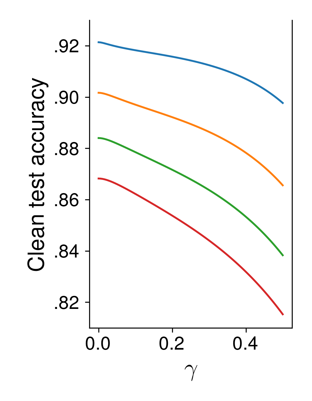
(a) clean test

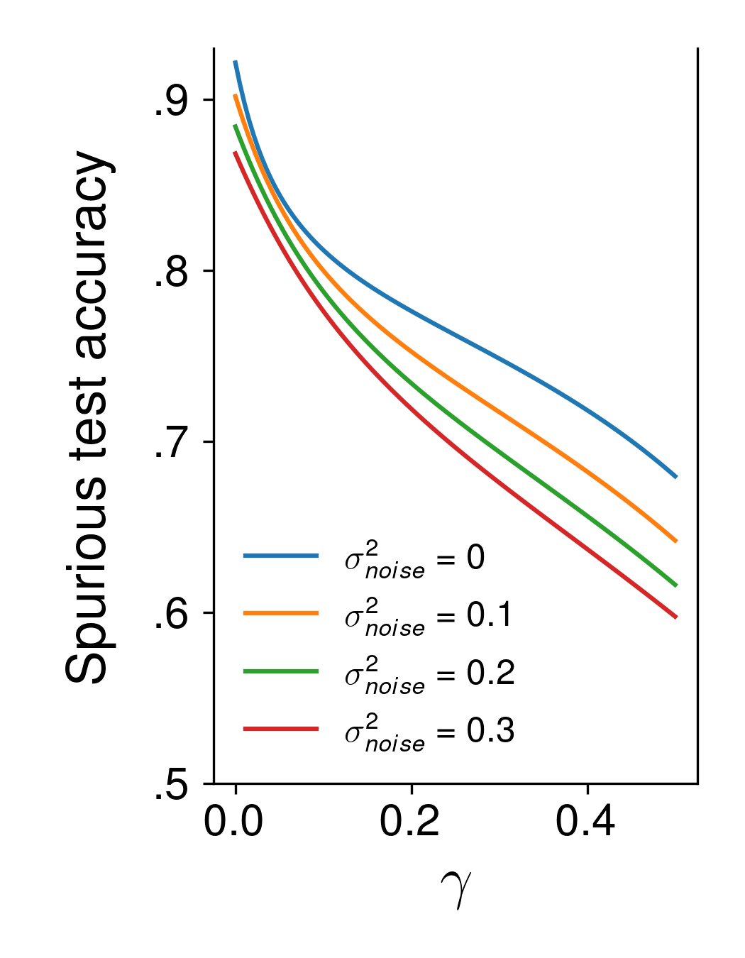
(b) spurious test

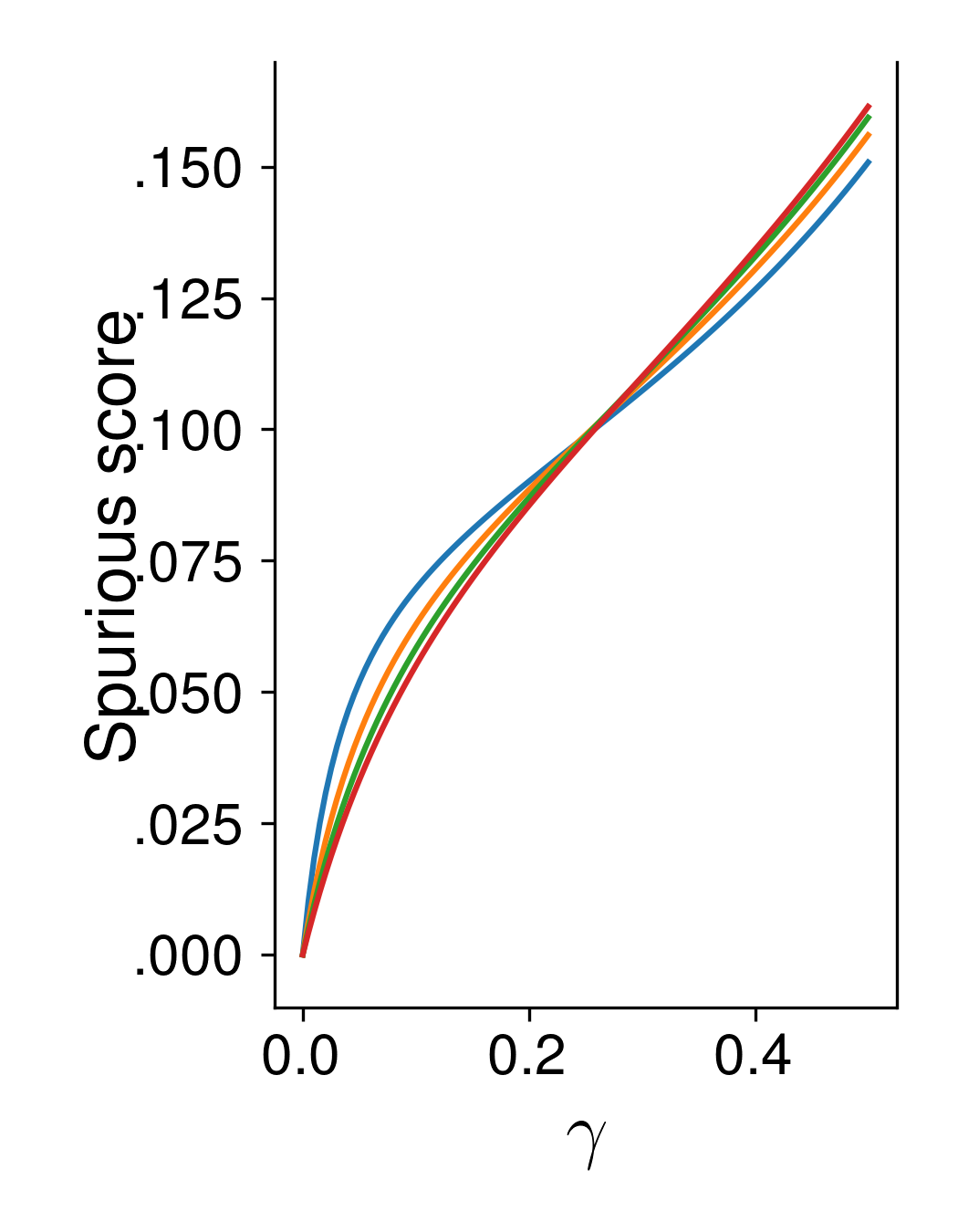
(c) spurious score

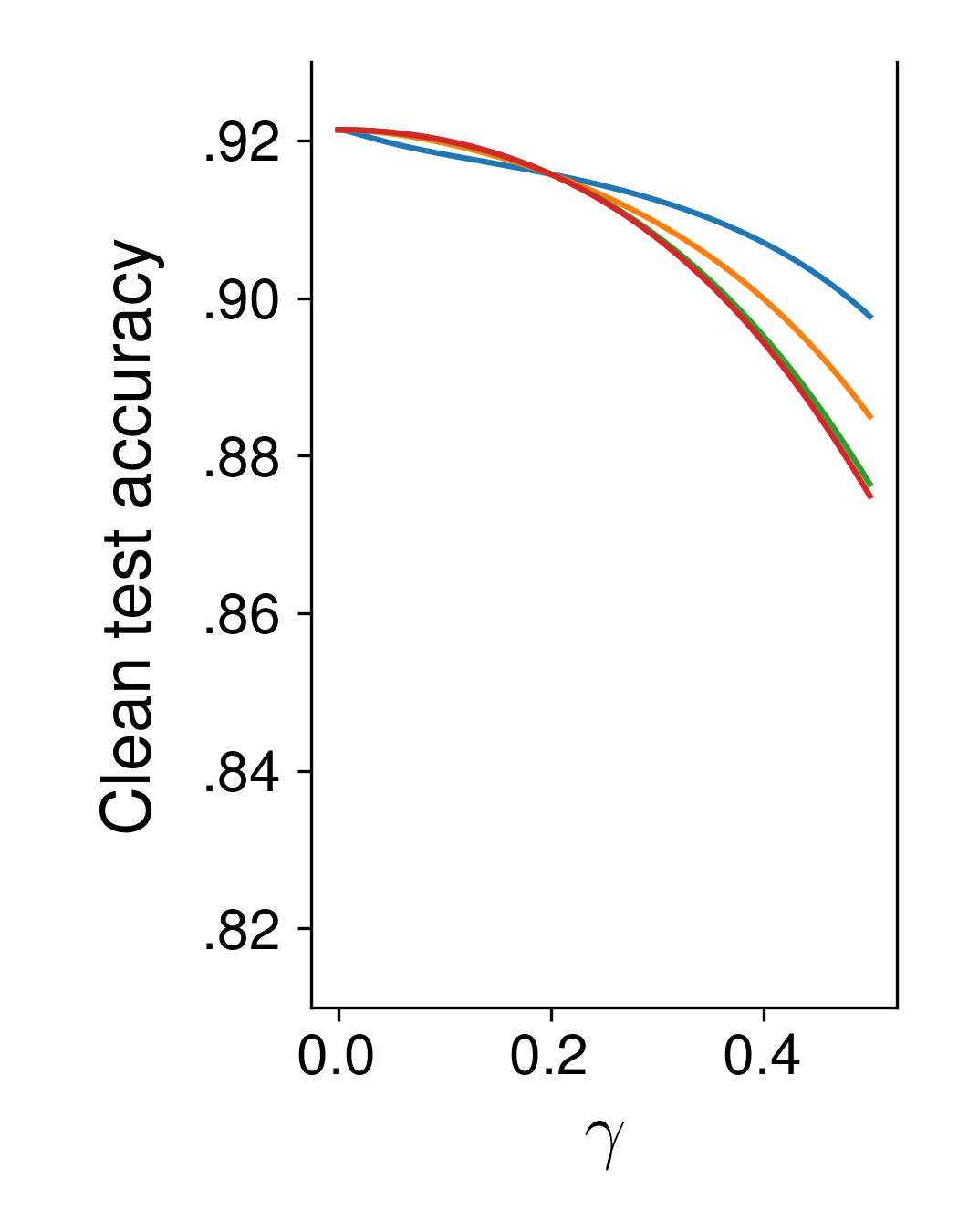
(d) clean test

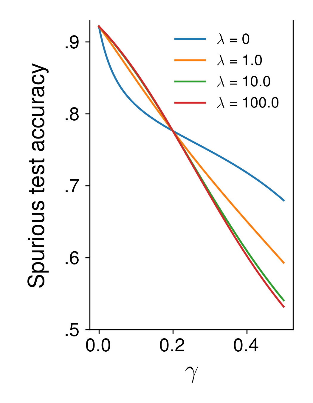
(e) spurious test

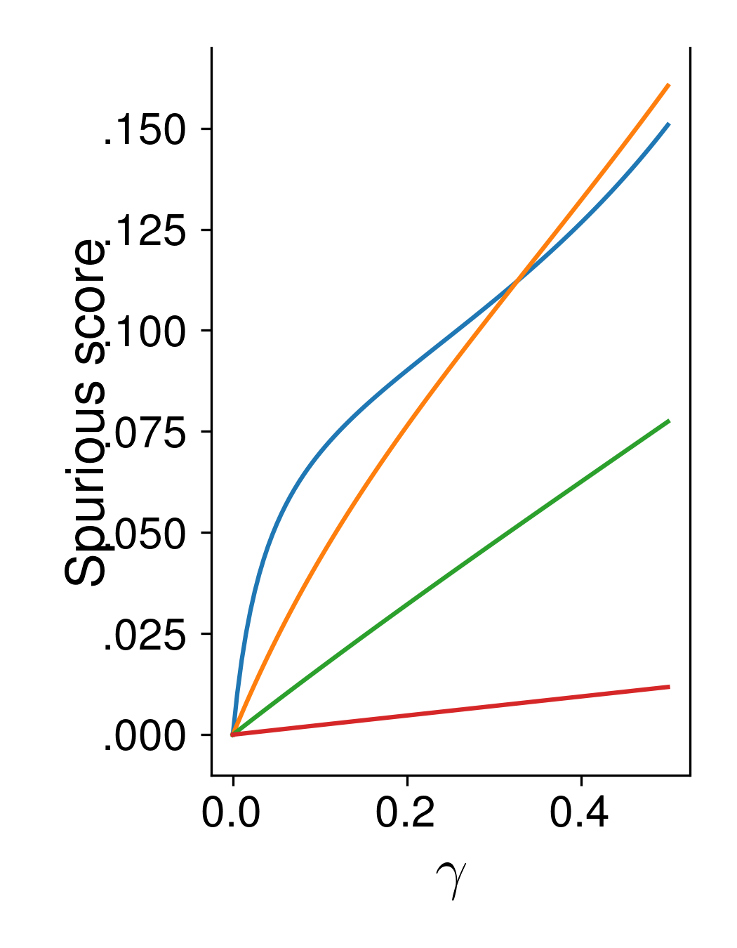
(f) spurious score

Figure 11: An example of our theoretical findings. (a)-(c): adding Gaussian noises. (d)-(f): $\ell_{2}$ regularization. The parameters are set to be $\|\mathbf{x}_{\text{sp}}\|_{2}^{2}=5$, $\sigma_{\text{inv}}^{2}=0.5$, $\sigma_{\text{sp}}^{2}=0.1$, and we consider $\gamma\in[0,0.5]$, noise strength $\sigma^{2}_{noise}=0,0.1,0.2,0.3$, and the $\ell_{2}$ regularization parameter $\lambda=0,1,10,100$.

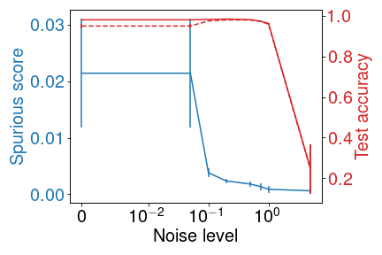
(a) MNIST, noisy input

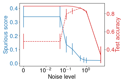
(b) Fashion, noisy input

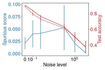
(c) CIFAR10, noisy input

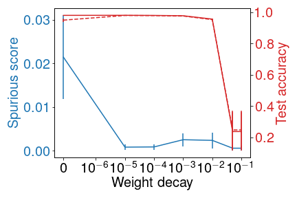
(d) MNIST, weight decay

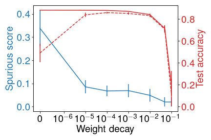
(e) Fashion, weight decay

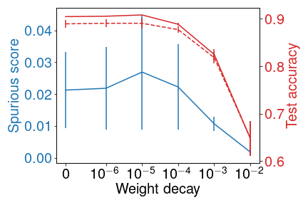
(f) CIFAR10, weight decay

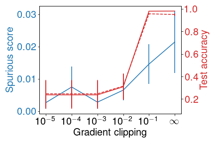
(g) MNIST, gradient clipping

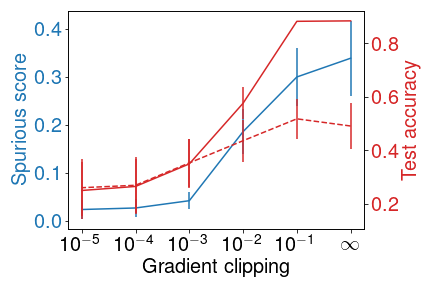
(h) Fashion, gradient clipping

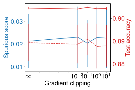
(i) CIFAR10, gradient clipping

Figure 12: Spurious score (solid blue line), clean test accuracy (solid red line), and spurious test accuracy (dotted red line) vs. the regularization strength on MNIST, Fashion, and CIFAR10 with different regularization methods. For the experiment, we fix the spurious pattern to be S3 and the target class $c_{tar}=0$. We compute the average spurious score and clean test accuracy across models trained with 1, 3, 5, 10, 20, and 100 spurious examples and five random seeds.

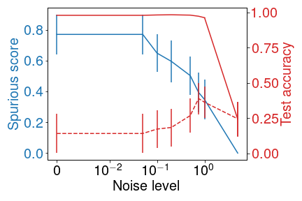
(a) MNIST, noisy input

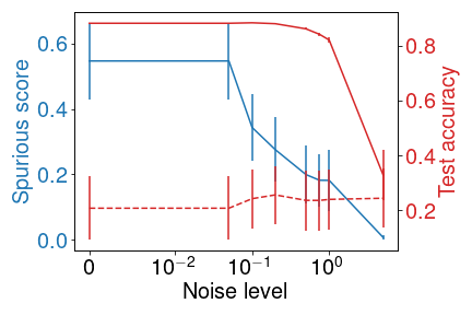
(b) Fashion, noisy input

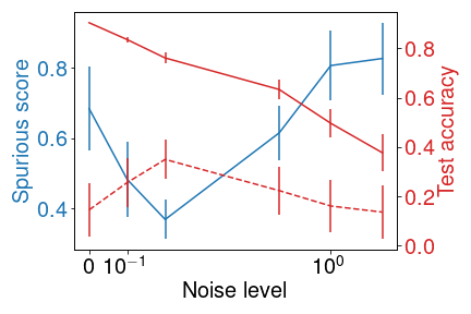
(c) CIFAR10, noisy input

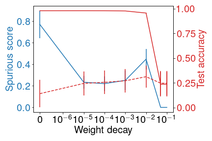
(d) MNIST, weight decay

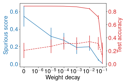
(e) Fashion, weight decay

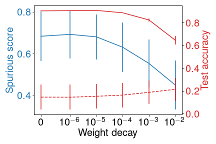
(f) CIFAR10, weight decay

(g) MNIST, gradient clipping

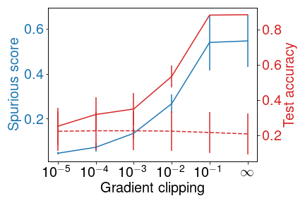
(h) Fashion, gradient clipping

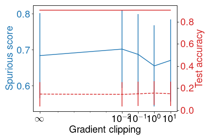
(i) CIFAR10, gradient clipping

Figure 13: Spurious score (solid blue line), clean test accuracy (solid red line), and spurious test accuracy (dotted red line) vs. the regularization strength on MNIST, Fashion, and CIFAR10 with different regularization methods. For the experiment, we fix the spurious pattern to be R3 and the target class $c_{tar}=0$. We compute the average spurious score and clean test accuracy across models trained with 1, 3, 5, 10, 20, and 100 spurious examples and five random seeds.

B.2 $\ell_{2}$ norm of the spurious pattern

In Fig. 2, we see that neural networks can learn different patterns very differently. For example, the spurious scores for R3 are higher than S1, suggesting spurious correlations with R3 are learnt more easily. Why does this happen? We hypothesize that the higher the norm of the pattern is, easier it is for a network to learn the correlation between the patterns and the target class.

Because the spurious patterns may overlap with other features, directly using the norm of each spurious pattern may not be accurate. We define the empirical norm of a spurious pattern $\mathbf{x}_{sp}$ on an example $\mathbf{x}$ as the $\ell_{2}$ distance between $\mathbf{x}$ and the spurious example $g(\mathbf{x},\mathbf{x}_{sp})$. We compute the average empirical norm over the test examples for each pattern. Tab. 1 shows the average empirical norm of each pattern on different datasets.

For each dataset, we train neural networks with a different number of spurious examples. To measure the aggregated effect of a spurious pattern across different numbers of spurious examples, we compute the average spurious scores across different numbers of spurious examples. We compute the Pearson correlation between the average empirical norm and the average spurious scores of each model trained with different spurious patterns. The testing results are: MNIST: $\rho=0.91$, $p<0.01$; Fashion: $\rho=0.84$, $p<0.02$; CIFAR10: $\rho=0.98$, $p<0.01$. The result shows a significantly strong positive correlation between the norm of the spurious patterns and the spurious scores.

Table 1: The average empirical norm of each spurious pattern.

	S1	S2	S3	R1	R2	R3	Inv
MNIST	1.00	3.00	5.00	3.88	7.70	15.19	5.98
Fashion	1.00	3.00	4.98	3.90	7.40	13.65	4.44
CIFAR10	0.84	2.57	4.34	7.72	14.54	23.20	8.00

B.3 Network architectures

Are some network architectures more susceptible to spurious correlations than others? To answer this question, we look at how spurious scores vary across different network architectures.

Network architectures. For MNIST and Fashion, we consider multi-layer perceptrons (MLP) with different sizes and a convolutional neural network (CNN). The small MLP has one hidden layer with $256$ neurons. The MLP has two hidden layers, each layer with $256$ neurons (the same MLP used in Fig. 2). The large MLP has two hidden layers, each with $512$ neurons. For CIFAR10, we consider ResNet20, ResNet34, ResNet110 (He et al., 2016), and Vgg16 Simonyan & Zisserman (2014). We use an SGD optimizer for CIFAR10 since we cannot get reasonable performance for Vgg16 with Adam.

Setup. For MNIST and Fashion, we set the learning rate to $0.01$ for all architectures and optimizers. We set the momentum to $0.9$ when the optimizer is SGD. For CIFAR10, when training with SGD, we set the learning rate to $0.1$ for ResNets trained and $0.01$ for Vgg16 because Vgg16 failed to converge with learning rate $0.1$. We set the learning rate to $0.01$ for ResNets when running with Adam (Vgg16 failed to converge with Adam). We use a learning rate scheduler which decreases the learning rate by a factor of $0.1$ on the $40$-th, $50$-th, and $60$-th epoch.

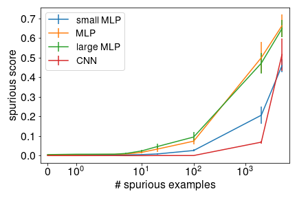
(a) MNIST, S3

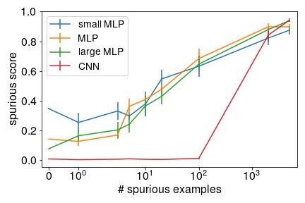
(b) Fashion, S3

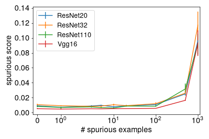
(c) CIFAR10, S3

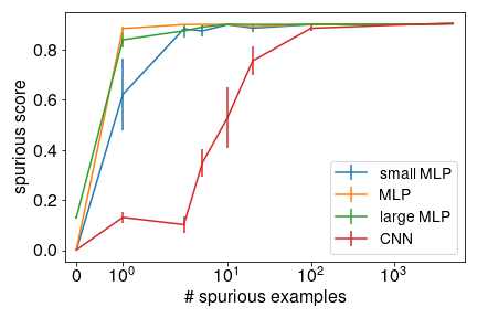
(d) MNIST, R3

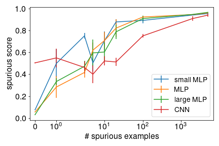
(e) Fashion, R3

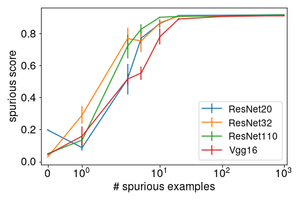
(f) CIFAR10, R3

Figure 14: The mean and standard error of the spurious scores with different network architectures on MNIST, Fashion, and CIFAR10. The target class is $c_{tar}=0$.

Fig. 14 shows the result, and we see that similar architectures with different sizes generally have similar spurious scores. Concretely, small MLP, MLP, and large MLP perform similarly, and ResNet20, ResNet32, and ResNet110 also perform similarly. Additionally, CNN is less affected by spurious examples than MLPs while Vgg16 is also slightly less affected than ResNets.

Why are MLPs more sensitive to small patterns? We observe that for S3, MLP seems to be the only architecture that can learn the spurious correlation when the number of spurious examples is small ($<100$). At the same time, CNN requires slightly more spurious examples while ResNets and Vgg16 cannot learn the spurious correlation on small patterns (note that the y-axis on Fig. 14 (e) is very small). Why is this happening? We hypothesize that different architectures have different sensitivities to the presence of evidence, i.e., the pixels of the image. Some architectures change their prediction a lot based on a small number of pixels, while others require a large number. If a network architecture is sensitive to changes in a small number of pixels, it can also be sensitive to a small spurious pattern.

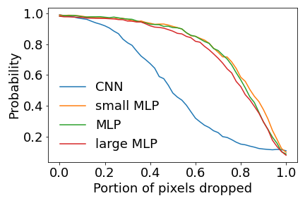
(a) MNIST

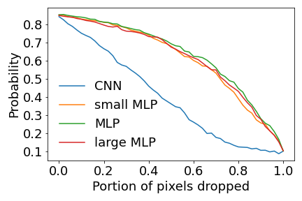
(b) Fashion

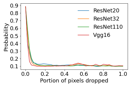
(c) CIFAR10

Figure 15: This figure shows the predicted probability of the ground truth label as a function of the portion of non-zero value pixels removed across different architectures and datasets.

To validate our hypothesis, we measure the sensitivity of a neural network as follows. First, we train a neural network on the clean training dataset. During testing, we set to zero $0\%,2\%,\ldots,98\%,100\%$ of randomly chosen non-zero pixels in each test image, and measure the predicted probability of its ground truth label. If this predicted probability continues to be high, then we say that the network is insensitive to the input. Fig. 15 shows the average predicted probability over $500$ training examples as a function of the percentage of pixels set to zero for the MNIST dataset.

We see that MLPs have around $0.9$ average predicted probability with half of the pixels zero-ed out. In contrast, the average predicted probability is lower in CNNs, suggesting that CNNs may be more sensitive to the zero-ed out pixels. From these results, we can rank the sensitivity of different architectures from non-sensitive to sensitive as MLPs $<$ CNN $<$ ResNets $\approx$ Vgg. This order matches our observation that MLPs are the most susceptible to spurious correlations, while CNN, ResNets, and Vgg16 are less so – suggestions that sensitive models may be more susceptible to learning spurious correlations with small patterns.

Finally, we find that architectures that have more parameters are not always more vulnerable to spurious correlations. Tab. 2 shows the number of parameters for each architecture. We see that while CNN has more parameters than small MLP, it is less susceptible to spurious correlations. Vgg16 and ResNet20 show a similar pattern. This observation is counter to Sagawa et al. (2020), who suggest that neural networks with more parameters can learn spurious correlations more easily, and it may be because they are looking at a different type of spurious correlation.

Table 2: Number of parameters in each architecture.

small MLP	MLP	large MLP	CNN
203,530	335,114	932,362	312,202
ResNet20	ResNet32	ResNet110	Vgg16
269,722	464,154	1,727,962	134,301,514

B.4 Optimization process

We study how the optimization process affects the learning of the spurious correlation. We look into two main components of the optimization process, the optimizers and the use of gradient clipping, and examine how each component affects the spurious score. For the optimizers, we compare between Adam and SGD, while for gradient clipping, we compare between no gradient clipping and clipping the norm the gradient to $0.1$. We repeat the five times with different random seeds and record their mean and standard error.

Fig. 17 shows the average spurious scores between different optimizers on different datasets and spurious patterns. We find that Adam is slightly more susceptible to spurious correlations than SGD, and gradient clipping does not affect the results much.

Fig. 17 shows the average spurious scores on networks trained with and without gradient clipping on different datasets and spurious patterns. We see that, in most cases, with and without gradient clipping performs similarly. It appears that using gradient clipping alone is not sufficient to eliminate the rare spurious correlations from neural networks.

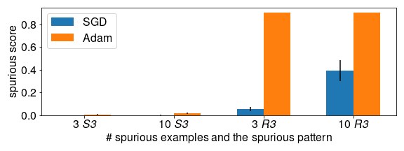
(a) MNIST SGD vs. Adam

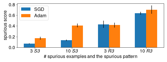
(b) Fashion SGD vs. Adam

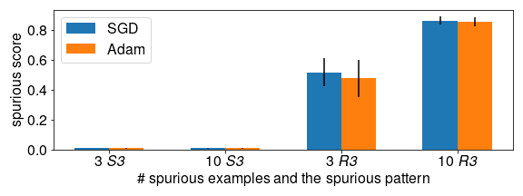
(c) CIFAR10 SGD vs. Adam

Figure 16: The mean and standard error of the spurious scores on neural networks trained with SGD versus Adam. We consider networks trained with three and ten spurious examples as well as using the S3 and R3 patterns.

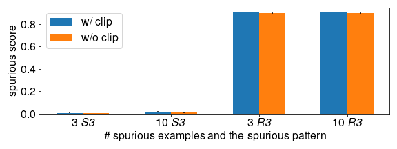
(a) MNIST w/ vs. w/o clipping

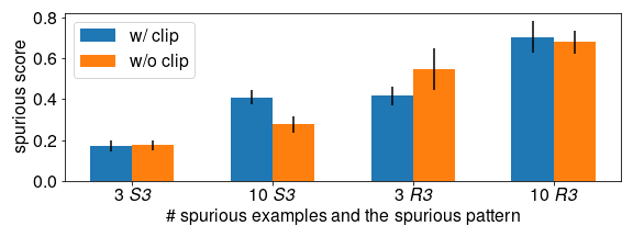
(b) Fashion w/ vs. w/o clipping

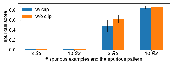
(c) CIFAR10 w/ vs. w/o clipping

Figure 17: The mean and standard error of the spurious scores on neural networks trained with and without gradient clipping. We consider networks trained with three and ten spurious examples as well as using the S3 and R3 patterns.

Overall, we see that rare spurious correlations are learnt regardless of the choice of the optimizer and whether the gradient clipping is performed or not. This indicates that tweaking individual components in the optimization process may not be sufficient to remove spurious correlations.

Appendix C Can Rare Spurious Correlations be Removed through Data Deletion Methods?

There has been a growing body of recent work on data deletion methods Koh et al. (2019); Izzo et al. (2021). Privacy laws such as the GDPR allow individuals to request an entity to remove their data, which includes removing it from any trained machine learning model. Since retraining models from scratch may be computationally expensive, a body of work has looked into developing more efficient methods. Here, we will look at two simple and canonical methods – incremental retraining and group influence (Koh et al., 2019; Basu et al., 2020b) that approximate the model that is trained without the deleted data points. Incremental retraining continues the training process for a number of epochs on the training data minus the deleted data, which effectively down weights the deleted data point in training. The group influence function computes a first-order approximation to the model that is trained without the deleted data point, motivated by influence functions from robust statistics. Both methods apply when multiple data points are deleted.

If all examples with a particular spurious pattern were deleted from the training set, then the spurious pattern and the target class should not be correlated in the resulting network. Therefore, we expect that a good data deletion method, when given a trained network and all training examples with a specific spurious pattern, should remove the associated spurious correlation from the network. In this section, we next investigate whether this is indeed the case.

Setup. We follow the same setup as in Fig. 2. We fix the spurious pattern to be R3, which is the pattern that gives the strongest correlation. We train the networks with $3$, $5$, $10$, $20$, and $100$ spurious examples. We apply two data deletion methods, incremental retraining and group influence, to the trained network. Each method takes in the trained network and the spurious training examples, and generates a new network that approximates the network that is trained on a training set without the spurious examples. We then measure the spurious scores for three types of models – the model before data deletion, model processed with incremental retraining, and model processed with group influence.

For incremental retraining, we continue the retraining process for $70$ epochs on the data minus the spurious examples (recall that the original models were also trained for $70$ epochs). For group influence, we adapt a publicly available implementation for data deletion.

Results. Fig. 18 shows the results. We see that for all three datasets, the models processed by the data deletion methods have similar spurious scores as the models before deletion. This implies that the spurious correlations remain even after “data deletion”, suggesting that these data deletion methods may not be effective at properly removing spurious examples. This has two implications – first, that rare spurious correlations, once introduced, may be challenging to remove. A second implication is that some data deletion methods may not properly remove all traces of the deleted data. We suggest that as a sanity check, future data deletion methods should test whether rare spurious correlations corresponding to the deleted examples are removed.

Finally, we note that there is a class of indistinguishable data deletion algorithms (Ginart et al., 2019; Neel et al., 2020) that provably ensure by adding noise that the deleted model is statistically indistinguishable from full retraining on the training data after deletion. However, these algorithms mostly apply to simpler problems, and we do not have efficient guaranteed deletion for non-convex problems such as training neural networks.

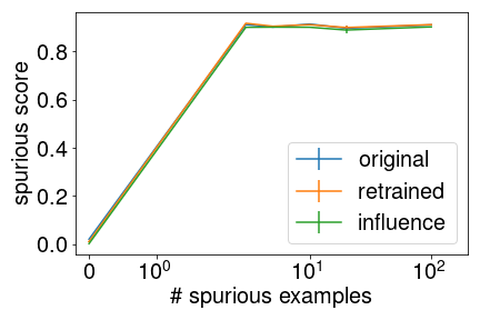
(a) MNIST

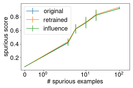
(b) Fashion

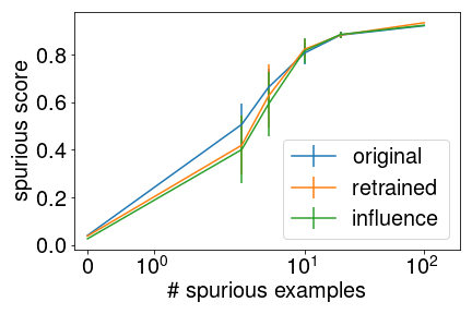
(c) CIFAR10

Figure 18: The mean and standard error of spurious scores of the original models, models after incremental retraining, and models after the group influence method. The choice of spurious pattern is R3, $c_{tar}=0$, and the optimizer is Adam. The lines for original and retrained are jittered by a small amount so that they are not completely overlapped.

Appendix D Experimental Details and Additional Results

The experiments are performed on six NVIDIA GeForce RTX 2080 Ti and two RTX 3080 GPUs located on three servers. Two of the servers have Intel Core i9 9940X and 128GB of RAM and the other one has AMD Threadripper 3960X and 256GB of RAM. All neural networks are implemented under the PyTorch framework (Paszke et al., 2019). Other packages, including numpy (Harris et al., 2020), scipy (Virtanen et al., 2020), tqdm, and pandas (pandas development team, 2020), are also used.

D.1 Experimental setup for Section 3

Architectures. For MNIST and Fashion, we consider multi-layer perceptrons (MLP) with ReLU activation functions. MLP has two hidden layers, and each layer has $256$ neurons. For CIFAR10, we consider ResNet20 (He et al., 2016).

Optimizer, learning rate, and data augmentation. We use the Adam (Kingma & Ba, 2014) optimizer and set the initial learning rate to $0.01$ for all models. We train the model for $70$ epochs. For the learning rate schedule, we decrease the learning rate by a factor of $0.1$ on the $40$-th, $50$-th, and $60$-th epoch. For CIFAR10, we apply data augmentation during training. When an image is passed in, we pad each border with four pixels and randomly crop the image to $32$ by $32$. We then, with $0.5$ probability, horizontally flip the image.

D.2 Experimental setup for Section 4

Membership inference attack setup. We split each dataset into four equally sized sets – target model training/testing sets and shadow model training/testing sets. We then add spurious features to a number of examples in the target model training set. We train the target model using the target model training set and the shadow model using the shadow model training set. Next, we extract the features on the target/shadow model training/testing sets. The feature we use are the output of the target/shadow model on these data and a binary indicator indicating whether the example is correctly predicted as the features. We then train an attack model (binary classifier) to distinguish whether an example comes from the shadow model training or testing sets using the extracted features. For evaluation, we compute the accuracy of the attack model distinguishing whether an example comes from the target model training or testing sets (test accuracy).

For the shadow and target model, we train them the same way as other models in Sec. 3. For the attack model, we use a logistic regression implemented with scikit-learn  (Pedregosa et al., 2011) with $3$-fold cross-validation to select the regularization parameter from $\{0.01,0.1,1.0,10.0\}$.

Appendix E Other Additional Results

The experimental code is available at https://github.com/yangarbiter/rare-spurious-correlation.

E.1 Additional results for qualitative analysis: visualizing network weights

Normalized feature importance. In Fig. 3, we show the original value of the importance for each pixel. For completeness, we present Fig. 19, which scales each pixel’s value to $[0,1]$ for each sub-figure. From the figure, we can still see that a small number of spurious examples can cause the learnt weight to change.

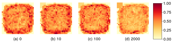
Figure 19: A normalized version of Fig. 19 (the values of each pixel is scaled to [0, 1] for each figure independently).

E.2 Additional results for $c_{tar}=1$

Results for another target class. For the completeness of Fig. 2, we show the results for $c_{tar}=1$ in Fig. 20. We see that in all these cases, increasing regularization strength decreases spurious scores The conclusions that can be made here are similar to ones made in Sec. 3 Fig. 2.

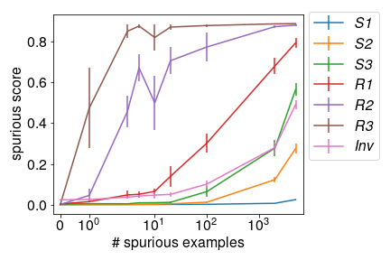
(a) MNIST, $c_{tar}=1$

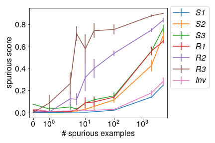
(b) Fashion, $c_{tar}=1$

(c) CIFAR10, $c_{tar}=1$

Figure 20: Each figure shows the mean and standard error of the spurious scores on three datasets, MNIST, Fashion, and CIFAR10, $c_{tar}=1$, and different numbers of spurious examples. In these figures, we use MLP as the network architecture for MNIST and Fashion, and we use ResNet20 for CIFAR10.

Results for clean test accuracy For completeness, we report the clean test accuracy for different number of spurious examples in Fig. 21. From the figures, we see that the clean test accuracy does not get affected too much as the number of spurious example grows. This aligns with our observation in Sec. 4, in which we see that the minimum and maximum clean test accuracy across all runs of experiments are close. This is as expected as the spurious examples are only presented in a small portion of the training data while accuracy measures average behavior.

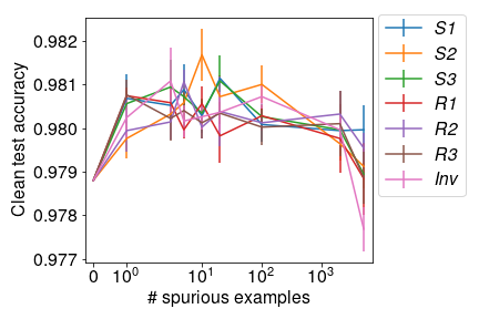
(a) MNIST, $c_{tar}=1$

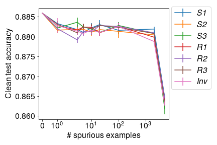
(b) Fashion, $c_{tar}=1$

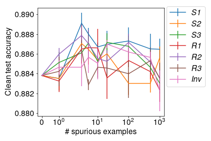
(c) CIFAR10, $c_{tar}=1$

Figure 21: Each figure shows the mean and standard error of the clean test accuracy on three datasets, MNIST, Fashion, and CIFAR10, $c_{tar}=0$, and different numbers of spurious examples. In these figures, we use MLP as the network architecture for MNIST and Fashion, and we use ResNet20 for CIFAR10.

E.3 Membership inference experiment with other spurious patterns

In Fig. 5, we show the results of the membership inference experiment while using R3 as the spurious pattern. For completeness, we show the results of attacking models trained on datasets with different spurious patterns in Fig. 22.

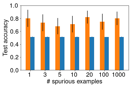
(a) MNIST, S1

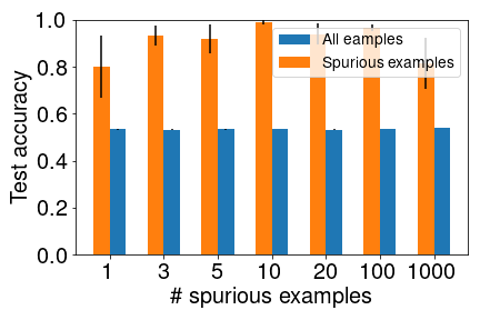
(b) Fashion, S1

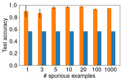
(c) CIFAR10, S1

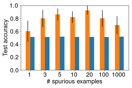
(d) MNIST, S2

(e) Fashion, S2

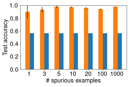
(f) CIFAR10, S2

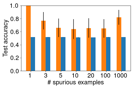
(g) MNIST, S3

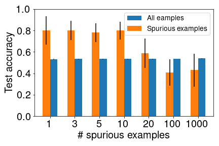
(h) Fashion, S3

(i) CIFAR10, S3

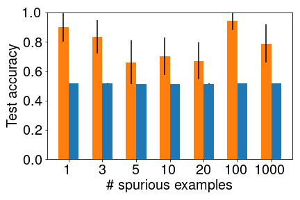
(j) MNIST, R1

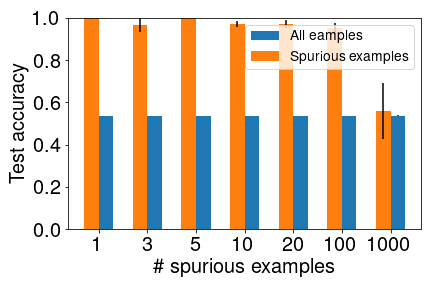
(k) Fashion, R1

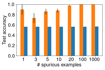
(l) CIFAR10, R1

(m) MNIST, R2

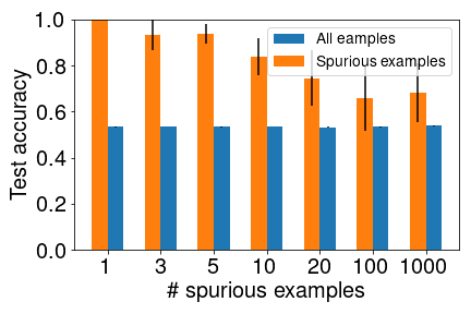
(n) Fashion, R2

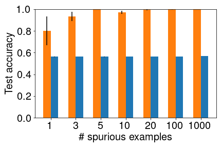
(o) CIFAR10, R2

(p) MNIST, R3

(q) Fashion, R3

(r) CIFAR10, R3

Figure 22: Additional results with all spurious patterns ($c_{\text{tar}}=1$) for the membership inference experiments (partial results are in Fig. 5).

E.4 Additional results for spurious test accuracy

For the completeness of Fig. 6, we show all results of the spurious test accuracy in Fig. 23.

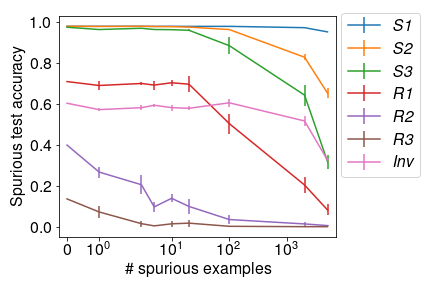
(a) MNIST, $c_{\text{tar}}=1$

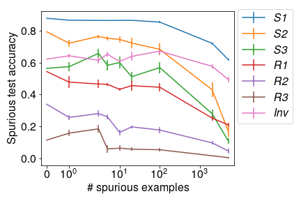
(b) Fashion, $c_{\text{tar}}=1$

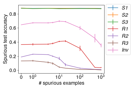
(c) CIFAR10, $c_{\text{tar}}=1$

Figure 23: Additional results on the spurious test accuracy over Fig. 6.

E.5 Natural rare spurious correlation

Fig. 24 shows the results for using dim and grass context as the spurious context. From the result, in all cases, spurious correlations are significantly learnt by neural networks with just $100$ spurious examples (less than $.2\%$ of the training data). We see that there are some cases spurious correlations are more easily learnt. For example, under the case where the dim context is the spurious context, two out of three spurious classes gets effected by $10$ spurious examples, and under Grass context with bicycle as the spurious class, it only requires $20$ spurious examples. These results confirms that natural spurious patterns can significantly effect a neural network.

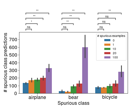
(a) Dim

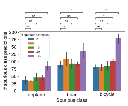
(b) Grass

Figure 24: The number of test examples that does not belongs to the spurious class gets predicted as the spurious class. We conduct Welch’s t-test (Welch, 1947) on the number of spurious class predictions between the model trained without spurious examples and models trained with different number of spurious examples. The notations for the p-values: ns$:0.05<p\leq 1.$, *$:10^{-2}<p\leq 0.05$, **$:10^{-3}<p\leq 10^{-2}$, ***$:10^{-4}<p\leq 10^{-3}$, ****$:p\leq 10^{-4}$.

E.6 Ablation studies

Normalized spurious score. A question is whether changing the scale of the spurious score (Eq. 1) could change the results in Fig. 2. In Fig. 25, we show a similar figure as Fig. 2 but with the y-axis switched to the normalized spurious score Eq. 5. From the figures, we see similar trend as of Fig. 2, and we can reach a similar conclusion as using the spurious score.

$$\frac{f_{c_{\text{tar}}}(\Phi_{\mathcal{X}}(\mathbf{x},\mathbf{x}_{\text{sp}}))-f_{c_{\text{tar}}}(\mathbf{x})}{f_{c_{\text{tar}}}(\Phi_{\mathcal{X}}(\mathbf{x},\mathbf{x}_{\text{sp}}))}>\epsilon\ .$$ (5)

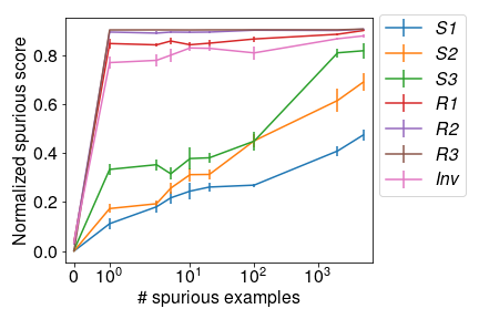
(a) MNIST, $c_{\text{tar}}=0$

(b) Fashion, $c_{\text{tar}}=0$

(c) CIFAR10, $c_{\text{tar}}=0$

Figure 25: Results of the normalized spurious score (Eq. 5) with different number of spurious examples on MNIST, Fashion, and CIFAR10.

Appendix F Additional Related Work and Discussions

Short-cut learning (Geirhos et al., 2020; Yu et al., 2021) and simplicity bias (Shah et al., 2020). The major difference between these works and our work is that they mainly focus on when spurious correlations are learned. They are less concerned with how rare these spurious correlations are, which is different from the focus of our work.

Backdoor attack. Our experiment procedure is similar to the data poisoning process applied in the backdoor attack. However, the context and message of our study are different from that of backdoor attacks in the following three ways. First, the spurious examples are not adversarial and, most of the time, are natural and simple. Second, our analysis is done on soft prediction, while backdoor attack focuses on hard label prediction. This allows us to observe results such as one spurious example that can significantly impact the model and its privacy implications, as these changes can be too subtle to be observed in a hard label setting.

Finally, we focus on a more fine-grained quantitative study on how the number of appearances of spurious training examples affects the performance of neural networks. The prior backdoor attack works often study a fixed poisoning rate (translates to having a fixed portion of the spurious examples in the training set). More specifically, (Li et al., 2021; Wu & Wang, 2021; Nam et al., 2020) focus on $0.1\%$ of training examples, which translates to 50 spurious examples for CIFAR10. Although they also study a small portion of the training set, their results are unable to provide insights on when the neural network begins to be affected by these spurious examples. In addition, we study the impact of different regularization methods (weight decay, noisy inputs, and gradient clipping), different optimizers (SGD vs. Adam, which makes a difference), and different architectures (CNN vs. MLP). These aspects had not been rigorously studied in previous work.

Data deletion methods. Inspired by GDPR, there are many recent works on data deletion. Izzo et al. (2021) demonstrate data deletion for linear classifiers but not for non-linear models such as neural networks. The use of influence and group influence functions for data deletion is also studied by many Koh & Liang (2017); Koh et al. (2019); Basu et al. (2020b). Basu et al. (2020a) point out that influence functions can be fragile for deeper neural networks. Our work shows that influence functions cannot remove spurious correlations caused by the deleted examples, which is different.

Concerns for expanding training sets. Researchers have also discovered ways that more data can hurt the model in terms of the generalization ability and test time accuracy (Nakkiran et al., 2019; Min et al., 2020). In this work, we uncover a different way that more data can hurt: more data could introduce more spurious correlations.

Comparison with other works related to memorization. There are works related to the memorization of a small number of special examples in the training set. Carlini et al. (2019) focus on language generative models. For generative models, they assign a likelihood to each input, which directly indicates whether an example is likely to appear or not. However, the likelihood for classification models indicates whether an example belongs to a certain class. Therefore, from this work alone, we are not able to conclude whether the classification model suffers from similar privacy issues. Nasr et al. (2021) and Jagielski et al. (2020) consider how in a worst-case scenario malicious inputs can cause privacy issues. However, our study focuses on whether natural spurious patterns can cause privacy issues. Although some steps for performing the experiment are similar, we focus on different aspects.

Mitigation of rare spurious correlations. There are existing works on defense against backdoor attacks and de-biasing neural networks, which are related to mitigating specific spurious correlations. One significant difference between these works and our work is that these works usually make some assumptions or use certain additional properties based on their application. For example, Li et al. (2021) assume that spurious examples in the training set have a lower training loss than clean examples, Wu & Wang (2021) assume that backdoor-related neurons are also more sensitive to adversarial perturbations, and Nam et al. (2020) assume the spurious (biased) examples are harder to learn (one can start to see some contradiction between (Li et al., 2021) and (Nam et al., 2020) as spurious examples may be easier or harder to learn in different settings). These assumptions may work well in specific settings. But, there are no guarantees on whether they will work on other kinds of spurious patterns (or backdoor attacks).

In our work, we take a more general perspective and do not make any assumptions besides the fact that spurious examples are rare. Here are some intuitions on how regularization methods can help with mitigating rare spurious correlations. For weight decay (which is the same as regularization), it effectively puts a penalty on every weight that is greater than zero. Therefore, it discourages the neural network from putting weights on features that occur rarely. For noise injection, it is inspired by the differential privacy literature. Differential privacy is often achieved by adding noise during training, and by doing so, one can make the model less affected by a small group of training examples. Finally, we use gradient clipping as a baseline to show that not all kinds of regularization methods are useful in mitigating rare spurious correlations.

Relationship with adversarial examples. One nice connection to adversarial examples is that if rare spurious correlations are present in the training data, an adversary can introduce them in a test point to bring down the classification accuracy. Our experiments in Fig. 22 actually illustrate this. In that sense, the adversary in our experiment is, in fact, a highly constrained test-time adversary (who can only apply a specific pattern to test inputs).

An interesting hypothesis is that some adversarial examples can be caused by rare spurious correlations. This suggests a future direction in examining the relationship between the inserted spurious pattern and the direction of the adversarial perturbations (Goodfellow et al., 2014). One related work is from Weng et al. (2020), who suggests that “by increasing the robustness of a network to adversarial examples, the network becomes more vulnerable to backdoor attacks.” Backdoor attacks also insert a small portion of specifically designed spurious patterns into the training set. Thus, robustness to backdoor attacks can be related to the spurious correlation we are measuring. Their result indicates that there exist adversarial examples that are not purely caused by rare spurious examples.

Further discussions on Fig. 6. In the figure, there are cases where the spurious test accuracy does not drop for a fairly large number of spurious examples. There are two implications: 1) As in these cases, even though the spurious test accuracy does not drop, we still see that spurious examples are more vulnerable to the membership inference attack (see Fig. 5). This means that there are cases where the hard predictions of the neural network cannot measure whether the spurious correlations are learned. 2) This implies that different spurious patterns can have different effects on different datasets/architectures. One interesting future direction is to figure out when spurious examples are more effective and when it is less effective.

References

- Abadi et al. (2016) Martin Abadi, Andy Chu, Ian Goodfellow, H Brendan McMahan, Ilya Mironov, Kunal Talwar, and Li Zhang. Deep learning with differential privacy. In Proceedings of the 2016 ACM SIGSAC conference on computer and communications security, pp. 308–318, 2016.
- Arjovsky et al. (2019) Martin Arjovsky, Léon Bottou, Ishaan Gulrajani, and David Lopez-Paz. Invariant risk minimization. arXiv preprint arXiv:1907.02893, 2019.
- Arpit et al. (2017) Devansh Arpit, Stanisław Jastrzebski, Nicolas Ballas, David Krueger, Emmanuel Bengio, Maxinder S Kanwal, Tegan Maharaj, Asja Fischer, Aaron Courville, Yoshua Bengio, et al. A closer look at memorization in deep networks. In International Conference on Machine Learning, pp. 233–242, 2017.
- Bahng et al. (2020) Hyojin Bahng, Sanghyuk Chun, Sangdoo Yun, Jaegul Choo, and Seong Joon Oh. Learning de-biased representations with biased representations. In International Conference on Machine Learning, pp. 528–539, 2020.
- Basu et al. (2020a) Samyadeep Basu, Philip Pope, and Soheil Feizi. Influence functions in deep learning are fragile. arXiv preprint arXiv:2006.14651, 2020a.
- Basu et al. (2020b) Samyadeep Basu, Xuchen You, and Soheil Feizi. On second-order group influence functions for black-box predictions. In International Conference on Machine Learning, pp. 715–724, 2020b.
- Burkard & Lagesse (2017) Cody Burkard and Brent Lagesse. Analysis of causative attacks against svms learning from data streams. In Proceedings of the 3rd ACM on International Workshop on Security And Privacy Analytics, pp. 31–36, 2017.
- Carlini et al. (2019) Nicholas Carlini, Chang Liu, Úlfar Erlingsson, Jernej Kos, and Dawn Song. The secret sharer: Evaluating and testing unintended memorization in neural networks. In 28th USENIX Security Symposium (USENIX Security 19), pp. 267–284, 2019.
- Carlini et al. (2020) Nicholas Carlini, Florian Tramer, Eric Wallace, Matthew Jagielski, Ariel Herbert-Voss, Katherine Lee, Adam Roberts, Tom Brown, Dawn Song, Ulfar Erlingsson, et al. Extracting training data from large language models. arXiv preprint arXiv:2012.07805, 2020.
- Chang et al. (2021) Chun-Hao Chang, George Alexandru Adam, and Anna Goldenberg. Towards robust classification model by counterfactual and invariant data generation. In Proceedings of the IEEE/CVF Conference on Computer Vision and Pattern Recognition, pp. 15212–15221, 2021.
- Chaudhuri et al. (2011) Kamalika Chaudhuri, Claire Monteleoni, and Anand D Sarwate. Differentially private empirical risk minimization. Journal of Machine Learning Research, 12(3), 2011.
- Chen et al. (2017) Xinyun Chen, Chang Liu, Bo Li, Kimberly Lu, and Dawn Song. Targeted backdoor attacks on deep learning systems using data poisoning. arXiv preprint arXiv:1712.05526, 2017.
- Dwork et al. (2006) Cynthia Dwork, Frank McSherry, Kobbi Nissim, and Adam Smith. Calibrating noise to sensitivity in private data analysis. In Theory of cryptography conference, pp. 265–284, 2006.
- Feldman & Zhang (2020) Vitaly Feldman and Chiyuan Zhang. What neural networks memorize and why: Discovering the long tail via influence estimation. arXiv preprint arXiv:2008.03703, 2020.
- Geirhos et al. (2020) Robert Geirhos, Jörn-Henrik Jacobsen, Claudio Michaelis, Richard Zemel, Wieland Brendel, Matthias Bethge, and Felix A Wichmann. Shortcut learning in deep neural networks. Nature Machine Intelligence, 2(11):665–673, 2020.
- Ginart et al. (2019) Antonio Ginart, Melody Y Guan, Gregory Valiant, and James Zou. Making ai forget you: Data deletion in machine learning. arXiv preprint arXiv:1907.05012, 2019.
- Goodfellow et al. (2014) Ian J Goodfellow, Jonathon Shlens, and Christian Szegedy. Explaining and harnessing adversarial examples. arXiv preprint arXiv:1412.6572, 2014.
- Gururangan et al. (2018) Suchin Gururangan, Swabha Swayamdipta, Omer Levy, Roy Schwartz, Samuel R Bowman, and Noah A Smith. Annotation artifacts in natural language inference data. arXiv preprint arXiv:1803.02324, 2018.
- Harris et al. (2020) Charles R. Harris, K. Jarrod Millman, Stéfan J. van der Walt, Ralf Gommers, Pauli Virtanen, David Cournapeau, Eric Wieser, Julian Taylor, Sebastian Berg, Nathaniel J. Smith, Robert Kern, Matti Picus, Stephan Hoyer, Marten H. van Kerkwijk, Matthew Brett, Allan Haldane, Jaime Fernández del Río, Mark Wiebe, Pearu Peterson, Pierre Gérard-Marchant, Kevin Sheppard, Tyler Reddy, Warren Weckesser, Hameer Abbasi, Christoph Gohlke, and Travis E. Oliphant. Array programming with NumPy. Nature, 585(7825):357–362, September 2020. doi: 10.1038/s41586-020-2649-2. URL https://doi.org/10.1038/s41586-020-2649-2.
- Hartley & Tsaftaris (2022) John Hartley and Sotirios A Tsaftaris. Measuring unintended memorisation of unique private features in neural networks. arXiv preprint arXiv:2202.08099, 2022.
- He et al. (2016) Kaiming He, Xiangyu Zhang, Shaoqing Ren, and Jian Sun. Deep residual learning for image recognition. In Proceedings of the IEEE conference on computer vision and pattern recognition, pp. 770–778, 2016.
- Idrissi et al. (2021) Badr Youbi Idrissi, Martin Arjovsky, Mohammad Pezeshki, and David Lopez-Paz. Simple data balancing achieves competitive worst-group-accuracy. arXiv preprint arXiv:2110.14503, 2021.
- Izzo et al. (2021) Zachary Izzo, Mary Anne Smart, Kamalika Chaudhuri, and James Zou. Approximate data deletion from machine learning models. In International Conference on Artificial Intelligence and Statistics, pp. 2008–2016, 2021.
- Jagielski et al. (2020) Matthew Jagielski, Jonathan Ullman, and Alina Oprea. Auditing differentially private machine learning: How private is private sgd? Advances in Neural Information Processing Systems, 33:22205–22216, 2020.
- Khani & Liang (2021) Fereshte Khani and Percy Liang. Removing spurious features can hurt accuracy and affect groups disproportionately. In Proceedings of the 2021 ACM Conference on Fairness, Accountability, and Transparency, pp. 196–205, 2021.
- Kingma & Ba (2014) Diederik P Kingma and Jimmy Ba. Adam: A method for stochastic optimization. arXiv preprint arXiv:1412.6980, 2014.
- Koh & Liang (2017) Pang Wei Koh and Percy Liang. Understanding black-box predictions via influence functions. In International Conference on Machine Learning, pp. 1885–1894. PMLR, 2017.
- Koh et al. (2019) Pang Wei Koh, Kai-Siang Ang, Hubert HK Teo, and Percy Liang. On the accuracy of influence functions for measuring group effects. arXiv preprint arXiv:1905.13289, 2019.
- Krizhevsky & Hinton (2009) Alex Krizhevsky and Geoffrey Hinton. Learning multiple layers of features from tiny images, 2009.
- Kulynych et al. (2022) Bogdan Kulynych, Yao-Yuan Yang, Yaodong Yu, Jarosław Błasiok, and Preetum Nakkiran. What you see is what you get: Distributional generalization for algorithm design in deep learning. arXiv preprint arXiv:2204.03230, 2022.
- LeCun (1998) Yann LeCun. The mnist database of handwritten digits. http://yann. lecun. com/exdb/mnist/, 1998.
- Leino & Fredrikson (2020) Klas Leino and Matt Fredrikson. Stolen memories: Leveraging model memorization for calibrated white-box membership inference. In 29th USENIX Security Symposium (USENIX Security 20), pp. 1605–1622, 2020.
- Li et al. (2021) Yige Li, Xixiang Lyu, Nodens Koren, Lingjuan Lyu, Bo Li, and Xingjun Ma. Anti-backdoor learning: Training clean models on poisoned data. Advances in Neural Information Processing Systems, 34:14900–14912, 2021.
- Liu et al. (2018) Ziwei Liu, Ping Luo, Xiaogang Wang, and Xiaoou Tang. Large-scale celebfaces attributes (celeba) dataset. Retrieved August, 15(2018):11, 2018.
- Min et al. (2020) Yifei Min, Lin Chen, and Amin Karbasi. The curious case of adversarially robust models: More data can help, double descend, or hurt generalization. arXiv preprint arXiv:2002.11080, 2020.
- Nagarajan et al. (2020) Vaishnavh Nagarajan, Anders Andreassen, and Behnam Neyshabur. Understanding the failure modes of out-of-distribution generalization. arXiv preprint arXiv:2010.15775, 2020.
- Nakkiran et al. (2019) Preetum Nakkiran, Gal Kaplun, Yamini Bansal, Tristan Yang, Boaz Barak, and Ilya Sutskever. Deep double descent: Where bigger models and more data hurt. arXiv preprint arXiv:1912.02292, 2019.
- Nam et al. (2020) Junhyun Nam, Hyuntak Cha, Sungsoo Ahn, Jaeho Lee, and Jinwoo Shin. Learning from failure: De-biasing classifier from biased classifier. Advances in Neural Information Processing Systems, 33:20673–20684, 2020.
- Nasr et al. (2021) Milad Nasr, Shuang Songi, Abhradeep Thakurta, Nicolas Papemoti, and Nicholas Carlin. Adversary instantiation: Lower bounds for differentially private machine learning. In 2021 IEEE Symposium on Security and Privacy (SP), pp. 866–882. IEEE, 2021.
- Neel et al. (2020) Seth Neel, Aaron Roth, and Saeed Sharifi-Malvajerdi. Descent-to-delete: Gradient-based methods for machine unlearning. arXiv preprint arXiv:2007.02923, 2020.
- pandas development team (2020) The pandas development team. pandas-dev/pandas: Pandas, February 2020. URL https://doi.org/10.5281/zenodo.3509134.
- Paszke et al. (2019) Adam Paszke, Sam Gross, Francisco Massa, Adam Lerer, James Bradbury, Gregory Chanan, Trevor Killeen, Zeming Lin, Natalia Gimelshein, Luca Antiga, et al. Pytorch: An imperative style, high-performance deep learning library. Advances in neural information processing systems, 32, 2019.
- Pedregosa et al. (2011) F. Pedregosa, G. Varoquaux, A. Gramfort, V. Michel, B. Thirion, O. Grisel, M. Blondel, P. Prettenhofer, R. Weiss, V. Dubourg, J. Vanderplas, A. Passos, D. Cournapeau, M. Brucher, M. Perrot, and E. Duchesnay. Scikit-learn: Machine learning in Python. Journal of Machine Learning Research, 12:2825–2830, 2011.
- Sablayrolles et al. (2020) Alexandre Sablayrolles, Matthijs Douze, Cordelia Schmid, and Hervé Jégou. Radioactive data: tracing through training. In International Conference on Machine Learning, pp. 8326–8335, 2020.
- Sagawa et al. (2019) Shiori Sagawa, Pang Wei Koh, Tatsunori B Hashimoto, and Percy Liang. Distributionally robust neural networks for group shifts: On the importance of regularization for worst-case generalization. arXiv preprint arXiv:1911.08731, 2019.
- Sagawa et al. (2020) Shiori Sagawa, Aditi Raghunathan, Pang Wei Koh, and Percy Liang. An investigation of why overparameterization exacerbates spurious correlations. In International Conference on Machine Learning, pp. 8346–8356, 2020.
- Shah et al. (2020) Harshay Shah, Kaustav Tamuly, Aditi Raghunathan, Prateek Jain, and Praneeth Netrapalli. The pitfalls of simplicity bias in neural networks. Advances in Neural Information Processing Systems, 33:9573–9585, 2020.
- Shokri et al. (2017) Reza Shokri, Marco Stronati, Congzheng Song, and Vitaly Shmatikov. Membership inference attacks against machine learning models. In 2017 IEEE symposium on security and privacy (SP), pp. 3–18. IEEE, 2017.
- Simonyan & Zisserman (2014) Karen Simonyan and Andrew Zisserman. Very deep convolutional networks for large-scale image recognition. arXiv preprint arXiv:1409.1556, 2014.
- Srivastava et al. (2020) Megha Srivastava, Tatsunori Hashimoto, and Percy Liang. Robustness to spurious correlations via human annotations. In International Conference on Machine Learning, pp. 9109–9119, 2020.
- Virtanen et al. (2020) Pauli Virtanen, Ralf Gommers, Travis E. Oliphant, Matt Haberland, Tyler Reddy, David Cournapeau, Evgeni Burovski, Pearu Peterson, Warren Weckesser, Jonathan Bright, Stéfan J. van der Walt, Matthew Brett, Joshua Wilson, K. Jarrod Millman, Nikolay Mayorov, Andrew R. J. Nelson, Eric Jones, Robert Kern, Eric Larson, C J Carey, İlhan Polat, Yu Feng, Eric W. Moore, Jake VanderPlas, Denis Laxalde, Josef Perktold, Robert Cimrman, Ian Henriksen, E. A. Quintero, Charles R. Harris, Anne M. Archibald, Antônio H. Ribeiro, Fabian Pedregosa, Paul van Mulbregt, and SciPy 1.0 Contributors. SciPy 1.0: Fundamental Algorithms for Scientific Computing in Python. Nature Methods, 17:261–272, 2020. doi: 10.1038/s41592-019-0686-2.
- Wang & Chaudhuri (2018) Yizhen Wang and Kamalika Chaudhuri. Data poisoning attacks against online learning. arXiv preprint arXiv:1808.08994, 2018.
- Welch (1947) Bernard L Welch. The generalization of ‘student’s’problem when several different population varlances are involved. Biometrika, 34(1-2):28–35, 1947.
- Weng et al. (2020) Cheng-Hsin Weng, Yan-Ting Lee, and Shan-Hung Brandon Wu. On the trade-off between adversarial and backdoor robustness. Advances in Neural Information Processing Systems, 33:11973–11983, 2020.
- Wu & Wang (2021) Dongxian Wu and Yisen Wang. Adversarial neuron pruning purifies backdoored deep models. Advances in Neural Information Processing Systems, 34:16913–16925, 2021.
- Xiao et al. (2017) Han Xiao, Kashif Rasul, and Roland Vollgraf. Fashion-mnist: a novel image dataset for benchmarking machine learning algorithms. arXiv preprint arXiv:1708.07747, 2017.
- Xiao et al. (2015) Huang Xiao, Battista Biggio, Blaine Nelson, Han Xiao, Claudia Eckert, and Fabio Roli. Support vector machines under adversarial label contamination. Neurocomputing, 160:53–62, 2015.
- Xiao et al. (2020) Kai Xiao, Logan Engstrom, Andrew Ilyas, and Aleksander Madry. Noise or signal: The role of image backgrounds in object recognition. arXiv preprint arXiv:2006.09994, 2020.
- Yeom et al. (2017) Samuel Yeom, Matt Fredrikson, and Somesh Jha. The unintended consequences of overfitting: Training data inference attacks. arXiv preprint arXiv:1709.01604, 12, 2017.
- Yu et al. (2021) Da Yu, Huishuai Zhang, Wei Chen, Jian Yin, and Tie-Yan Liu. Indiscriminate poisoning attacks are shortcuts. arXiv preprint arXiv:2111.00898, 2021.
- Zhang et al. (2022) Xingxuan Zhang, Linjun Zhou, Renzhe Xu, Peng Cui, Zheyan Shen, and Haoxin Liu. Nico++: Towards better benchmarking for domain generalization. arXiv preprint arXiv:2204.08040, 2022.
- Zhou et al. (2021) Chunting Zhou, Xuezhe Ma, Paul Michel, and Graham Neubig. Examining and combating spurious features under distribution shift. In Proceedings of the 38th International Conference on Machine Learning, volume 139 of Proceedings of Machine Learning Research, pp. 12857–12867, Jul 2021.