Spoiler Susceptibility in Multi-District Party Elections

Abstract.

Electoral spoilers are such agents that there exists a coalition of agents whose total gain when a putative spoiler is eliminated exceeds that spoiler’s share in the election outcome. So far spoiler effects have been analyzed primarily in the context of single-winner electoral systems. We consider this problem in the context of multi-district party elections. We introduce a formal measure of a party’s excess electoral impact, treating “spoilership” as a manner of degree. This approach allows us to compare multi-winner social choice rules according to their degree of spoiler susceptibility. We present experimental results, as well as analytical results for toy models, for seven classical rules ($k$-Borda, Chamberlin–Courant, Harmonic-Borda, Jefferson–D’Hondt, PAV, SNTV, and STV). Since the probabilistic models commonly used in computational social choice have been developed for non-party elections, we extend them to be able to generate multi-district party elections.

1. Introduction

In the context of single–winner elections, a spoiler is usually defined as a losing candidate whose removal would affect the outcome by changing the winner [9, 32] (although other definitions have also been put forward – see, e.g., [30]).

We are particularly interested in investigating spoiler effects in political elections to multi–member representative bodies (e.g., parliaments). Such elections are distinguished from other types of multi–winner elections primarily by their character as party elections. By party election we mean such an election that all candidates are affiliated with parties, and that the allocation of the winning positions (“seats”) among those parties, rather than the identity of the winners themselves, is the most important outcome of the election. Thus, spoiler effects should also be considered in terms of spoiler parties and party (rather than individual) results.

In this paper, we seek first to extend the definition of a spoiler to multi-winner party elections, and then to compare multi-winner social choice rules according to their degree of spoiler susceptibility. Such an extension involves a number of issues. First, there is no longer a single natural definition of winners and losers. Most measures of election outcome (such as seat shares or voting power) are non–binary, and many parties are likely to have non-zero seat shares. Second, since the probabilistic models commonly used in computational social choice have been developed for non-party elections, we need to extend them to be able to analyze party elections probabilistically.

1.1. Contribution

To address the issues described above, we propose a more general definition of spoilership. A party $j$ is considered a spoiler if there exists a set of parties such that if $j$ is eliminated, that coalition’s total share in the election outcome exceeds $j$’s original share. The measure of such excess can be considered to be a measure of the “degree of spoilership”.

This approach allows us to compare multi-winner social choice rules according to their degree of spoiler susceptibility. We analyze seven well–known rules: $k$–Borda, Chamberlin–Courant, Harmonic Borda, Jefferson–D’Hondt, $k$–PAV, SNTV, and STV. We only consider anonymous rules in which the election outcome can be unequivocally determined from the ordinal preferences alone. We focus on experimental results under several probabilistic models extending the statistical cultures commonly used in non-party elections: Impartial Culture, 1-D and 2-D spatial models, single–peaked models, and the Mallows model. In the Appendix, we also analyze a toy model with three parties and single-peaked preference profiles.

1.2. Related Work

While spoiler effects have long been a familiar subject in the field of voting theory, there have been relatively few attempts to formally define spoilers or to measure the immunity of electoral systems to spoilers. However, spoiler effects have been tangentially considered in classical social choice theory primarily in the context of stronger postulates such as independence of irrelevant alternatives [1, 46, 8] or candidate stability [19, 20, 22, 48] or otherwise distinct though related postulates such as the independence of clones [52].

In computation social choice, spoilers have been addressed from the point of view of electoral control problems [39, 35, 12, 24, 41, 23], in particular of the problems of Constructive-Control-by-Adding-Candidates (CCAC) and Constructive-Control-by-Deleting-Candidates (CCDC), and their destructive control counterparts (DCAC and DCDC). In constructive control problems we seek to alter the election outcome by making a specific candidate a unique winner, while in destructive control problems we seek to make that candidate a non-winner. In CAC problems that objective is to be achieved by adding spoiler candidates, while in CDC problems we restrict the set of candidates by deleting some. While closely related to our subject, those problems are distinct primarily because they treat the election outcome in binary terms of being a winner / non-winner which are inapposite in party elections. Moreover, research on control problems considers vulnerability to spoilers in terms of computational complexity of solving the control problems, while we focus on the expected impact of a spoiler.

Kaminski [32] has been the first to propose a generalized definition of a spoiler applicable to party elections. He focused primarily on the problem of defining the election outcome by distinguishing ways in which a potential spoiler can affect seat payoff in a politically significant manner. Thus, apart from classical spoilers (which affect the outcome by turning a majority winner, i.e., the player with a majority of seats, into a majority loser, while making another player a majority winner), he notes the existence of kingmaker spoilers (who turn a majority loser in an election with no majority winner into a majority winner), kingslayer spoilers (who turn a majority winner into a majority loser, but make no other player a majority winner), and valuegobbler spoilers (who affect the seat payoff of one player by an amount greater than their own seat payoff). Nonetheless, his approach, while representing an important step, has two substantial limitations: first, his enumeration of politically significant ways for a spoiler to affect the election outcome is by no means exhaustive, and second, distinguishing minor and major players, as well as identifying feasible vote redistributions, all require qualitative judgments.

2. Preliminaries

Traditional computational social choice models have focused on $n$ voters electing a $k$–member committee out of $m$ candidates. In our models, each candidate is also affiliated with one of $p$ parties, and we focus on the allocation of committee members among those parties. Moreover, there are $c$ electoral districts, with an election held in each district in parallel. The overall election outcome is usually obtained by aggregation of district–level outcomes. We further assume in our experimental models that the number of candidates affiliated with each party equals $k$, i.e., $m=pk$, and that the numbers $n$, $m$, and $k$ are constant across districts.

2.1. Notation

$[t]$:

For $t\in\mathbb{Z_{+}}$, let $[t]$ denote the set $\{1,\dots,t\}$.

$[S]^{k}$:

For a set $S$, let $[S]^{k}$ denote the set of $k$-subsets of $S$.

$\Delta_{n}$:

Let $\Delta_{n}$ denote an $n-1$-dimensional unit simplex, i.e., $\Delta_{n}:=\{\mathbf{x}\in\mathbb{R}_{+}^{n}:\sum_{i=1}^{n}x_{i}=1\}$.

$\langle x_{i}\rangle_{i=a}^{b}$:

Let $\langle x_{i}\rangle_{i=a}^{b}$ denote the average of $x_{i}$ over $i=a,\dots,b$, i.e.,

$$\langle x_{i}\rangle_{i=a}^{b}:=\frac{1}{b-a+1}\sum_{i=a}^{b}x_{i}.$$

$v_{(k)}$:

For a strict preference order $v$ on a set $C$, let $v_{(k)}$ denote the $k$-th highest ranked element of $C$ in $v$.

$x_{k}^{\downarrow}$:

For $\mathbf{x}\in\mathbb{R}^{n}$, let $x_{k}^{\downarrow}$ denote the $k$-th largest coordinate of $\mathbf{x}$.

$\mathbf{u}_{k,l}$:

Let the $l$-dimensional $k$–approval vector $\mathbf{u}_{k,l}$, $l\geq k$, be a vector of $k$ ones followed by $l-k$ zeroes:

$$\mathbf{u}_{k,l}:=(\overbrace{1,\dots,1}^{k},\overbrace{0,\dots,0}^{l-k}).$$

$\mathbf{b}_{k}$:

Let the $k$-dimensional Borda vector $\mathbf{b}_{k}$ be defined as

$$\mathbf{b}_{k}:=(k-1,k-2,\dots,0)/({k-1}).$$

$\mathbf{h}_{k}$:

Let the $k$-dimensional harmonic vector $\mathbf{h}_{k}$ be defined as

$$\mathbf{h}_{k}:=\left(1,\frac{1}{2},\dots,\frac{1}{k}\right).$$

2.2. Definitions

Definition 1 (Party election).

Let $C$ be a finite set of candidates, $m:=|C|$, and let $L(C)$ be a set of linear orders on $C$. Let $P:=\{\rho_{1},\dots,\rho_{p}\}$ be a finite set of parties, and let $a:C\rightarrow P$ be a party affiliation function. Finally, let the preference profile $V$ be an $n$-element sequence of votes, $v_{1},\dots,v_{n}\in L(C)$, $n\in\mathbb{N}$. We refer to the quadruple $E:=(C,P,a,V)$ as a party election.

Definition 2 (Multi-winner social choice function).

A $k$-winner social choice function is a function $\mathcal{R}$ that maps a party election to a set of winning $k$–subsets ($k$–committees) of $C$. An election is tied under the social choice function $\mathcal{R}$ if $|\mathcal{R}(V)|>1$.

Definition 3 (Allocation rule).

An allocation rule is a function that maps a party election into the probability simplex $\Delta_{p}$. Each $k$-winner social choice function $\mathcal{R}$ naturally induces an allocation rule $s_{\mathcal{R},k}$ such that the $i$-th coordinate of $s_{\mathcal{R},k}(V)$ equals $\langle|\{y\in S:a(y)=\rho_{i}\}|/k\rangle_{S\in\mathcal{R}(V)}$, where $i\in[p]$. Note this assumes that ties are resolved by choosing a winning committee randomly with a uniform distribution on $\mathcal{R}(V)$.

Definition 4 (OWA–based scoring rule).

An OWA–based scoring rule induced by an OWA vector $\mathbf{z}\in[0,1]^{k}$ and a scoring vector $\mathbf{w}\in[0,\infty)^{m}$, $\mathcal{R}^{\mathrm{OWA}}_{\mathbf{w},\mathbf{z}}$, is a social choice function that maps a party election to the set of all $k$–subsets of $C$ maximizing over $S\in C^{[k]}$ the expression $\sum_{v\in V}\sum_{i=1}^{k}z_{i}w_{\mathrm{pos}(v,S)_{i}}$, where $\mathrm{pos}(v,S)$ is a $k$–dimensional vector such that $\mathrm{pos}(v,S)_{i}$ is the position of the $i$–th highest ranked member of $S$ in $v$.

Definition 5 (Multi-district party election).

A $c$-district party election is a sequence $\boldsymbol{E}:=\{E_{1},\dots,E_{c}\}$, where $E_{j}:=(C_{j},P,a_{j},V_{j})$, $j\in[c]$.

Definition 6 (Multi-district allocation rule).

A $c$-district allocation rule is a function that maps a multi-district party election into the probability simplex $\Delta_{p}$.

2.3. Voting and Allocation Rules

We analyze seven allocation rules. Five of them are induced by OWA–based scoring rules [26, 27]:

Definition 7 (SNTV (plurality)).

Let $\mathcal{R}_{k}^{SNTV}:=\mathcal{R}^{\mathrm{OWA}}_{\mathbf{u}_{1,k},\mathbf{u}_{1,m}}$ be an OWA–based rule induced by the $1$-approval scoring vector $\mathbf{u}_{1,m}$ and the $1$-approval OWA–vector $\mathbf{u}_{1,k}$, i.e., such rule that maps a profile $V$ to a set of $k$–subsets of the set of candidates with scores not lesser than the $k$–th best scoring candidate according to the plurality scoring rule (where only the first position counts).

Definition 8 ($k$–Borda).

Let $\mathcal{R}_{k}^{Borda}:=\mathcal{R}^{\mathrm{OWA}}_{\mathbf{u}_{k,k},\mathbf{b}_{m}}$ be an OWA–based rule induced by a Borda scoring vector $\mathbf{b}_{m}$ and a $k$-approval OWA–vector $\mathbf{u}_{k,k}$, i.e., such rule that maps a profile $V$ to a set of $k$–subsets of the set of candidates with scores not lesser than the $k$–th best scoring candidate according to the Borda scoring rule (with uniformly decreasing position scores) [15, 25].

Definition 9 (Chamberlin–Courant (CC)).

Let $\mathcal{R}_{k}^{CC}:=\mathcal{R}^{\mathrm{OWA}}_{\mathbf{u}_{1,k},\mathbf{b}_{m}}$ be an OWA–based rule induced by a Borda scoring vector $\mathbf{b}_{m}$ and a $1$–approval OWA–vector $\mathbf{u}_{1,k}$, i.e., such rule that maps a profile $V$ to a set of $k$–subsets of the set of candidates maximizing the sum of Borda scores of the highest–ranking committee member [11].

Definition 10 (Harmonic Borda).

Let $\mathcal{R}_{k}^{HB}:=\mathcal{R}^{\mathrm{OWA}}_{\mathbf{h}_{k},\mathbf{b}_{m}}$ be an OWA–based rule induced by a Borda scoring vector $\mathbf{b}_{m}$ and a harmonic OWA–vector $\mathbf{h}_{k}$, i.e., such rule that maps a profile $V$ to a set of $k$–subsets of the set of candidates maximizing the sum of committee scores defined as the sum of the Borda scores of committee members with harmonically decreasing weights [25].

Definition 11 (Proportional $k$–Approval Voting).

Let $\mathcal{R}_{k}^{PAV}:=\mathcal{R}^{\mathrm{OWA}}_{\mathbf{h}_{k},\mathbf{u}_{k,m}}$ be an OWA–based rule induced by an $k$-approval scoring vector, $\mathbf{u}_{k,m}$, and a harmonic OWA–vector $\mathbf{h}_{k}$, i.e., such rule that maps a profile $V$ to a set of $k$–subsets of the set of candidates maximizing the sum of committee scores defined as the $j$-th harmonic number, $H_{j}$, where $j$ is the number of committee members included within the voter’s $k$ highest–ranked candidates [34, 51]. Note this rule differs from classical PAV by requiring each voter to approve exactly $k$ candidates.

We also consider two other allocation rules that are frequently encountered in real–life political elections:

Definition 12 (STV).

Let $\mathcal{R}_{k}^{STV}$ be a social choice function defined as follows: let $q:={n}/{(k+1)}$ be the fractional Droop quota, let initial vote weights be $1$, and let the committee $S$ and the set of discarded candidates $D$ be initially defined as empty sets. We iteratively rank the candidates according to the weighted number of votes in which they have been ranked highest of all candidates $c\in C\setminus(S\cup D)$, denoted for the $i$-th candidate as $t_{i}$. Let $Q:=\{c\in C\setminus(S\cup D):t_{c}\geq q\}$ be the set of the candidates for whom the number of such votes exceeds the quota. If $Q$ is non-empty, we add those candidates to the committee and multiply the weight of all votes cast for each candidate $c\in Q$ by $q/t_{c}$. If $Q$ is empty, we add the last–ranked candidate to $D$. The process is repeated until $|S|\geq k$, and the result is the set of all $k$–subsets of $S$ [29, 54].

Definition 13 (Jefferson–D’Hondt).

Let $r_{k}^{JDH}$ be an allocation rule defined as follows: let $w_{i}$, $i\in[p]$, be the share of votes such that the $i$-th party’s candidate is ranked first, and let $\mathcal{M}$ be such interval that for each $M\in\mathcal{M}$, $\sum_{i\in[p]}\lfloor Mw_{i}\rfloor=k$. Then the $i$-th coordinate of $r_{k}^{JDH}$ is given by $\lfloor Mw_{i}\rfloor/k$, where $M\in\mathcal{M}$ (the rule is independent of the choice of $M$) [31, 16, 17, 4, 45].

Remark 1.

If $\mathcal{M}$ is empty, an electoral tie occurs. For consistency with tie resolution in other voting rules, we can extend our definition of $r_{k}^{JDH}$ as follows: let $k_{+}\in\{j\in\mathbb{N}:j>k\}$ be the smallest such integer that there exists a non-empty interval $\mathcal{M}_{+}$ such that for each $M\in\mathcal{M}_{+}$, $\sum_{i\in P}\,\lfloor Mw_{i}\rfloor=k_{+}$, and let $k_{-}\in\{j\in\mathbb{N}:j<k\}$ be the greatest such integer that there exists a non-empty interval $\mathcal{M}_{-}$ such that for each $M\in\mathcal{M}_{-}$, $\sum_{i\in P}\lfloor Mw_{i}\rfloor=m_{-}$. Then the $i$-th coordinate of $r_{k}^{JDH}$ is given by:

$$\frac{k-k_{-}}{k_{+}-k_{-}}\frac{\lfloor M_{+}w_{i}\rfloor}{k_{+}}+\frac{k_{+}-k}{k_{+}-k_{-}}\frac{\lfloor M_{-}w_{i}\rfloor}{k_{-}},$$

where $M_{+}\in\mathcal{M}_{+}$ and $M_{-}\in\mathcal{M}_{-}$ (the rule is independent of the choice of $M_{+}$ and $M_{-}$).

Remark 2.

To simplify theoretical calculations, we can approximate the $i$–th coordinate of the multi–district Jefferson–D’Hondt allocation rule using the following formula [28]: Let parties be ordered degressively by $w_{i}$. Then

(1) $$s_{i}\approx\widehat{w}_{i}\left(1+\frac{r}{2k}\right)-\frac{1}{2k}$$

for $i=1,\dots,r$, where,

(2) $$r:=\max\left\{l\in[p]:\frac{w_{l}}{\sum_{j=1}^{l}w_{j}}>\frac{1}{2k+l}\right\},$$

$\widehat{w}_{i}$ is the renormalized vote share of the $i$-th party:

(3) $$\widehat{w}_{i}:={w_{i}}/\left({\sum{}_{j=1}^{r}w_{j}}\right).$$

Any family of allocation rules $r:=(r_{i},\dots,r_{c})$ induces a multi-district allocation rule $s$ given by the weighted average $s(\boldsymbol{E}):=(\sum_{i=1}^{c}k_{i}r_{i}(V_{i}))/(\sum_{i=1}^{c}k_{i})$, where $k_{i}\in\mathbb{N}_{+}$ is the number of seats allocated in the $i$-th district.

3. Measuring Spoiler Susceptibility

Intuitively, a restriction of an election to a subset $P^{\prime}$ is one in which candidate sets are restricted to candidates affiliated with parties in $P^{\prime}$, and others are eliminated from all votes.

Definition 14 (Restriction of an election).

Formally, let $\boldsymbol{E}:=\{E_{1},\dots,E_{c}\}$ be a $c$–district party election. We define a restriction of $\boldsymbol{E}$ to $P^{\prime}$, $\boldsymbol{E}_{P^{\prime}}:=\{E^{\sim}_{1},\dots,E^{\sim}_{c}\}$, with $P^{\prime}\subseteq P$, as a $c$–district party election such that $E^{\sim}_{j}:=\{C^{\prime}_{j},P^{\prime},a^{\prime}_{j},V^{\prime}_{j}\}$, $j\in[c]$, where:

1. $C^{\prime}_{j}$ is the preimage of $P^{\prime}$ under $a_{j}$, i.e., the set of candidates restricted to those affiliated with parties in $P^{\prime}$,

2. $a^{\prime}_{j}:=a_{j}\restriction_{C^{\prime}_{j}}$ is the restriction of $a$ to $C^{\prime}_{j}$,

3. $V^{\prime}_{j}:=(v_{j,1}\restriction_{C^{\prime}_{j}},\dots,v_{j,n}\restriction_{C^{\prime}_{j}})$.

We will denote $\boldsymbol{E}_{P\setminus\{i\}}$ by $\boldsymbol{E}_{-i}$.

Definition 15 (Redistribution region).

Let $\boldsymbol{E}$ be a $c$–district party election. A redistribution region of the $i$-th party, $R_{i}\subset\Delta_{p}$, is a set of possible redistributions of the $i$–th party’s share in the election outcome $\mathbf{s}$:

(4) $$R_{i}:=\left\{x\in\Delta_{p}:{\lVert\mathbf{x}-\mathbf{s}\rVert}_{1}\leq s_{i}\right\}.$$

Note that $R_{i}$ is a convex hull of $\{\mathbf{s}+s_{i}(\mathbf{e}_{j}-\mathbf{e}_{i}):j\neq i\}$, where vectors $\mathbf{e}_{1},\dots,\mathbf{e}_{p}$ are vertices of $\Delta_{p}$. Thus, $R_{i}$ is a regular $(p-2)$–dimensional simplex embedded in the facet $\{\mathbf{x}\in\Delta_{p}:x_{i}=0\}$.

Figure 1. Geometric interpretation of excess electoral impact.

Definition 16 (Excess electoral impact).

Let $\boldsymbol{E}$ be a $c$–district party election. We define the excess electoral impact of the $i$-th party as the $L_{1}$ distance between the outcome of the restriction $\boldsymbol{E}_{-i}$ and the redistribution region of $R_{i}$, see Fig. 1:

(5) $$\lambda_{i}^{s}(\boldsymbol{E}) :=\min_{\mathbf{x}\in R_{i}}{\left\lVert\mathbf{x}-s(\boldsymbol{E}_{-i})\right\rVert}_{1}$$

(6) $$={\left\lVert s(\boldsymbol{E})-s(\boldsymbol{E}_{-i})\right\rVert}_{1}-2s(\boldsymbol{E})_{i}.$$

Let us consider the set of parties that gain shares in the election outcome when party $i$ is eliminated, i.e., $L_{i}:=\{j\in[p]:s(\boldsymbol{E}_{-i})_{j}>s(\boldsymbol{E})_{j}\}$. Party $i$ has a non-zero excess electoral impact if and only if the total gains of parties in $L_{i}$ exceed $s(\boldsymbol{E})_{i}$. In such a case, we describe $i$ as a spoiler and parties $j\in L_{i}$ as spoilees. Note that the existence of spoilees implies that there also exist parties which lose shares in the election outcome when $i$ is eliminated.

Finally, we define spoiler susceptibility of a multi-district allocation rule as the expected maximum excess electoral impact, where the maximum is taken for each election over the set of parties, and the expectation is over some probability distribution on the set of profiles.

Definition 17 (Spoiler susceptibility).

Let $s$ be a multi-district allocation rule, and let $\mathcal{D}$ be a probability distribution on the set of elections with fixed $p$ and $c$. Finally, let $\boldsymbol{E}\sim\mathcal{D}$. Then the spoiler susceptibility of $s$ is given by:

(7) $$\Phi(\mathcal{D},s):=\mathbb{E}\,\max\limits_{i\in P}\lambda_{i}^{s}(\boldsymbol{E}).$$

To illustrate the definition, we present a real-life example.

4. Real-life Example (Polish election of 2015)

In the Polish general election of 2015, the Jefferson–D’Hondt rule has been used to allocate a total of 460 seats in 41 districts with the district magnitude parameter $m$ varying between $7$ and $20$. In addition, a statutory threshold has been set at $5\%$ of the total number of valid votes for parties and $8\%$ of the total number of valid votes for electoral coalitions. Only parties and coalitions whose vote shares exceeded the appropriate threshold participated in the seat allocation. There have been eight major contenders (see Table 1).

Using party position data from the Chapel Hill Expert Survey [2, 43, 3] we have mapped each party to a point $(x_{i},y_{i})$. We assume that if the $i$-th party were removed, its votes would have been redistributed among other parties, $j\neq i$, inversely proportionally to the Euclidean distances between points $(x_{j},y_{j})$ and $(x_{i},y_{i})$. Under this assumption, we have computed for each party $i=1,\dots,8$ the excess electoral impact $\lambda_{i}^{s}$ under the Jefferson–D’Hondt rule.

name	$w_{i}$	seats	$x_{i}$	$y_{i}$	$\lambda^{s}_{i}$
PiS	$.376$	$235$	$.295$	$.914$	$.000$
PO	$.241$	$138$	$.657$	$.467$	$.061$
Kukiz	$.088$	$42$	$.675$	$.761$	$.097$
Nowoczesna	$.076$	28	$.767$	$.261$	$.114$
Lewica (*)	$.076$	0	$.391$	$.357$	$.124$
PSL	$.051$	16	$.433$	$.710$	$.131$
Korwin	$.048$	0	$.906$	$.953$	$.144$
Razem	$.036$	0	$.129$	$.122$	$.184$

Table 1. Parties in the Polish general election of 2015, where $w_{i}$ is the vote share. Asterisk (*) denotes electoral coalitions.

We find that the left-wing party Razem has attained the highest excess electoral impact in our example. This is in accord with a common intuition that Razem has indeed acted as a spoiler, preventing its nearest neighbor Lewica from crossing the $8\%$ electoral threshold for coalitions and thus enabling the winning PiS party to attain a standalone majority. Lewica has been the main spoilee for Razem in this example, followed by Korwin and Nowoczesna.

5. Toy Models

Let us consider a following class of toy models: there are three parties, $P=\{X,Y,Z\}$, with $k$ candidates each, ordered as $X_{1}\ll\dots\ll X_{k}\ll Y_{1}\ll\dots\ll Y_{k}\ll Z_{1}\ll\dots\ll Z_{k}$. We assume that the preference profile is single-peaked with respect to $\ll$, and that the candidates of a single party are grouped together within each vote. Thus, there are $4\cdot 2^{k-1}$ possible votes – four admissible orderings on parties and, for each of them, $2^{k-1}$ admissible orderings on the candidates of the party that is ranked first (“peak party”). For other parties, candidate orders are determined by the choice of the peak party. We assign probabilities to those orders by first choosing the probabilities of the four party orderings, $\mathrm{Pr}_{X\prec Y\prec Z}$, $\mathrm{Pr}_{Z\prec Y\prec X}$, $\mathrm{Pr}_{X\prec Z\prec Y}$, and $\mathrm{Pr}_{Z\prec X\prec Y}$, and then fix the probabilities for each candidate ordering.

If the middle party were the largest one, or if all parties were of approximately equal size, the probability of spoiler effects would be relatively small, making the model uninteresting. Thus, we assume that one of the extreme parties – $Z$, without loss of generality – is the large party, i.e., is ranked first by the largest number of voters. We also assume that the probabilities of all orderings are unequal. Those two assumptions leave us with six configurations of parties, each of which is defined by an ordering on the coordinates of the vector $\mathbf{Q}:=(\mathrm{Pr}_{X\prec Y\prec Z},\mathrm{Pr}_{Z\prec Y\prec X},\mathrm{Pr}_{X\prec Z\prec Y},\mathrm{Pr}_{Z\prec X\prec Y})$ such that $\mathrm{Pr}_{X\prec Y\prec Z}$ is always the largest one.

An ordering of four probabilities corresponds to the division of a unit simplex $\Delta_{4}$ into $24$ asymmetric simplices. However, since $\mathrm{Pr}_{X\prec Y\prec Z}$ is always the largest of those four probabilities, only six of the asymmetric simplices will be of interest to us. For each configuration, we draw the vector of probabilities $\mathbf{Q}$ from the uniform distribution on the corresponding asymmetric simplex, thus ensuring the consistency of the ordering of the probabilities with the chosen configuration.

Ordering of the peak party’s candidates is fixed independently of the choice of the said party. We choose a fixed vector of probabilities $\mathbf{u}_{k}:=(u_{1}^{k},\dots,u_{2^{k-1}}^{k})$, where

$$u_{i}^{k}:=\frac{1}{2^{k-1}}\sum_{j=i}^{2^{k-1}}\frac{1}{j},$$

and $i=1,\dots,2^{k-1}.$

For any OWA–based rule, we can express the expected score for each $k$–committee $S$ as a linear combination of the probabilities assigned to each possible vote, and thus easily determine, for each of the enumerated configurations, seat allocations under the $k$–Borda, Chamberlin-Courant, Harmonic Borda, PAV, and SNTV rules for random single-district party elections $E_{\mathbf{Q}}:=(\{X,Y,Z\}\times[k],\{X,Y,Z\},a,V)$, where $a(x)=x_{1}$ (see the attached Mathematica notebook for source code). The random preference profile $V$ is drawn according to the distribution of votes determined by vector $\mathbf{Q}$ as described above. We likewise determine, for each such profile, seat allocations for $E_{\mathbf{Q}}$ to $[\{X,Y,Z\}]^{2}:=\{\{X,Y\},\{X,Z\},\{Y,Z\}\}$. Finally, using Definition 4 we obtain an expected maximum excess electoral impact for each rule under consideration.

$\mathrm{Pr}_{X\prec Y\prec Z}>\mathrm{Pr}_{Z\prec Y\prec X}>\mathrm{Pr}_{X\prec Z\prec Y}>\mathrm{Pr}_{Z\prec X\prec Y}$
$k=2$	PAV	Borda	HB	SNTV	CC
	.220	.166	.072	.066	.003
$k=3$	Borda	PAV	HB	SNTV	CC
	.176	.127	.043	.027	.000
$\mathrm{Pr}_{X\prec Y\prec Z}>\mathrm{Pr}_{Z\prec Y\prec X}>\mathrm{Pr}_{Z\prec X\prec Y}>\mathrm{Pr}_{X\prec Z\prec Y}$
$k=2$	Borda	HB	PAV	SNTV	CC
	.141	.085	.040	.013	.002
$k=3$	Borda	HB	PAV	SNTV	CC
	.138	.072	.040	.001	.000
$\mathrm{Pr}_{X\prec Y\prec Z}>\mathrm{Pr}_{X\prec Z\prec Y}>\mathrm{Pr}_{Z\prec Y\prec X}>\mathrm{Pr}_{Z\prec X\prec Y}$
$k=2$	PAV	Borda	SNTV	HB	CC
	.221	.079	.063	.030	.005
$k=3$	PAV	Borda	HB	SNTV	CC
	.127	.085	.023	.005	.000
$\mathrm{Pr}_{X\prec Y\prec Z}>\mathrm{Pr}_{X\prec Z\prec Y}>\mathrm{Pr}_{Z\prec X\prec Y}>\mathrm{Pr}_{Z\prec Y\prec X}$
$k=2$	PAV	Borda	SNTV	HB	CC
	.087	.065	.040	.032	.001
$k=3$	PAV	Borda	HB	SNTV	CC
	.130	.071	.026	.003	.000
$\mathrm{Pr}_{X\prec Y\prec Z}>\mathrm{Pr}_{Z\prec X\prec Y}>\mathrm{Pr}_{Z\prec Y\prec X}>\mathrm{Pr}_{X\prec Z\prec Y}$
$k=2$	Borda	HB	PAV	SNTV	CC
	.252	.153	.087	.042	.003
$k=3$	Borda	PAV	HB	SNTV	CC
	.254	.128	.118	.004	.000
$\mathrm{Pr}_{X\prec Y\prec Z}>\mathrm{Pr}_{Z\prec X\prec Y}>\mathrm{Pr}_{X\prec Z\prec Y}>\mathrm{Pr}_{Z\prec Y\prec X}$
$k=2$	Borda	HB	PAV	SNTV	CC
	.250	.166	.040	.014	.003
$k=3$	Borda	HB	PAV	SNTV	CC
	.244	.137	.040	.002	.000

Table 2. Voting rules ordered from the most to the least susceptible to spoiler effects for six toy models. Values below the name of the voting rule are the spoiler susceptibility indices of such voting rule.

The performance of the five social choice rules under consideration with respect to their susceptibility to spoiler effects depends strongly on the choice of the model, but we can note a number of regularities: Chamberlin–Courant is always most resistant to spoilers, followed usually by SNTV. Harmonic Borda is always more resistant to spoilers than $k$–Borda. Finally, $k$–Borda is the most spoiler-susceptible method, except where $\mathrm{Pr}_{X\prec Z\prec Y}$ is the second largest probability, in which case $k$–PAV takes its place.

6. Experiments

In this section we provide experimental results regarding spoilerity-resistance of different voting rules in practice. We start by describing probabilistic models that we use for generating election. Then, we present the results.

6.1. Probabilistic Models

The probabilistic models commonly used in computational social choice (see generally [6, 50]) have been developed for single-district non-party elections. In order to measure spoiler susceptibility of social choice rules used in multi-district party elections, we need to introduce appropriate extensions of those rules, addressing two basic challenges:

1. grouping of candidates into parties, and

2. existence of multiple electoral districts.

Grouping of candidates into parties is based on a latent assumption of intra-party candidate clustering: candidates of the same party, while not identical, are assumed to be perceived by voters as, on average, more similar than candidates of different parties. Accordingly, we would assume them to be usually (though not necessarily) clustered together in votes. Without that assumption, parties would tend to obtain roughly equal seat shares, leading to an overall electoral tie.

Existence of multiple electoral districts reflects another latent assumption – one of intra-district voter clustering. Voters within a single district are assumed not to constitute an unbiased sample of the population, but to share preferences to a greater extent. Without that assumption, the $c$-district allocation rule would (per the central limit theorem) converge (as $O(1/\sqrt{c})$) to the expected value of the allocation rule applied to the preference profile of the full population.

We consider four classes of probabilistic models:

Definition 18 (Spatial Models).

In a $d$-dimensional Euclidean model each party, voter, and candidate is assigned an ideal point in $\mathbb{R}^{d}$ [21, 40]. First, party ideal points are drawn from the uniform distribution on $(0,1)^{d}$, and then candidate ideal points for each district are drawn from the multivariate normal distribution with location at the party’s ideal point and the correlation matrix $\mathbf{\Sigma}:=\sigma I_{d}$, where $I_{d}$ is a $d\times d$ identity matrix and $\sigma\in\mathbb{R}_{+}$. Voter ideal points are drawn independently from the uniform distribution on $(0,1)^{d}$, and then shifted in each district independently by a shift vector drawn from a uniform distribution on $(-1/4,1/4)^{d}$ (to account for intra-district voter clustering). Finally, each vote is obtained by sorting candidates according to the increasing Euclidean ($L_{2}$) distance between the candidate’s and the voter’s ideal points.

Definition 19 (Single-Peaked Models).

We consider two models for the generation of single-peaked profiles. In the model proposed by Walsh [55] we are given an ordering on the set of candidates, and each vote is drawn from the uniform distribution on the set of all single-peaked votes consistent with that ordering. In the model proposed by Conitzer [13] the peak is drawn from a uniform distribution on candidates, and the remainder of the vote is obtained through a random walk. In both models, candidate ordering in each district is obtained in the same manner as in the $1$-dimensional Euclidean model described above, and there is no mechanism accounting for intra-district voter clustering.

Definition 20 (Mallows Model).

The Mallows model [37, 14] is parametrized by a single parameter $\phi\in[0,1]$, and a (central) vote $v_{c}\in L(C)$. The probability of generating a vote $v$ is proportional to $\phi^{f(v_{c},v)}$, where $f(v_{c},v)$ is the Kendall tau distance [33] between $v_{c}$ and $v$, i.e., the minimum number of swaps of adjacent candidates needed to transform the vote $v$ into the central vote $v_{c}$. We apply the Mallows model in two stages, first generating a central vote for each district, $v_{c}^{i}$ with parameter $\phi_{1}$ and an overall central vote $v_{c}^{0}:=[n]$, then generating votes within each district with parameter $\phi_{2}$ and a district–wide central vote $v_{c}^{i}$. Intra-party clustering is achieved by grouping party candidates together in the overall central vote. On sampling from the Mallows model, see [36].

For our simulations, we use a novel Mallows model parameterization proposed by Boehmer et al. [7], which instead of classical $\phi$ uses a normalized dispersion parameter ${{\mathrm{norm}\hbox{-}\phi}}$.

Definition 21 (Impartial Culture (IC)).

Under the Impartial Culture model, each vote is drawn randomly from the uniform distribution on $L(C)$, the set of linear orders on the set of candidates $C$, and there is no dependence between votes within or across districts [10]. This model is unable to account for intra-party and intra-district clustering, and is generally considered a poor approximation of real-life elections [47, 53], thus being only tested as a reference point.

6.2. Results

To compare voting methods, we analyze their performance under 11 probabilistic models: four spatial models ($d=1,2$ and $\sigma=0.05,0.2$), four single-peaked models (Walsh and Conitzer, $\sigma=0.05,0.2$), two Mallows models ($\phi_{1}=0.75$, $\phi_{2}=0.25,0.75$) and Impartial Culture. For every voting method, model, committee size $k\in\{1,5,15\}$, and number of parties $p\in\{3,\dots,10\}$ we run 600 simulations, with the number of districts $c=100$, and the number of voters per district $n=100$. For Jefferson–D’Hondt we use the Pot & Ladle approximation (see Appendix, Eq. 1), for SNTV, $k$-Borda, and STV we use the optimal algorithms, while for CC, HB, and $k$-PAV we use greedy approximation algorithms.

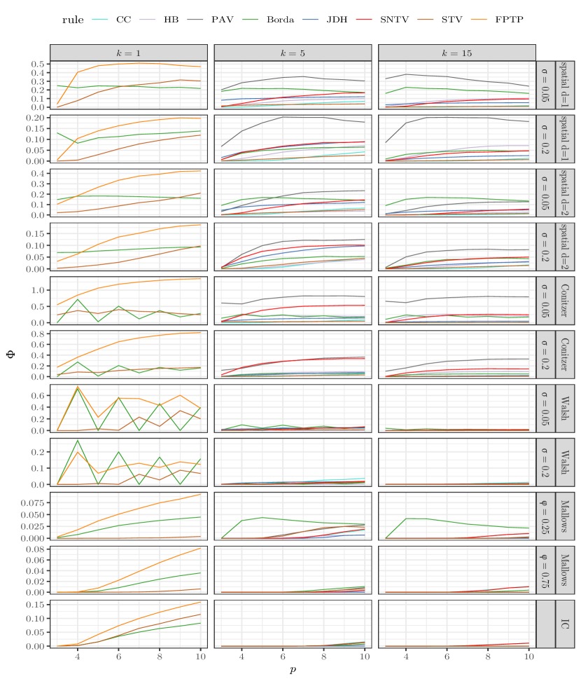
Figure 2. Spoiler susceptibility of electoral rules.

Experimental results plotted on Figure 2 demonstrate several regularities. First, spoiler susceptibility of social choice rules depends strongly on the choice of the probabilistic model. Under spatial models, which are most likely to approximate political elections, we can distinguish several classes of rules. Those least susceptible to spoilers are STV, Chamberlin–Courant (only in multi-member district models), and Harmonic Borda (only in multi-member district models with $d>1$). The ordering on them depends on the number of parties – CC outperforms STV for large values of $p$. SNTV and Jefferson-D’Hondt are the middle performers, with JDH becoming the more resistant rule as the number of parties increases. On the other hand, $k$–Borda performs poorly against spoilers in models with high degree of party clustering ($\sigma=0.05$), but is more spoiler–resistant than JDH and SNTV in models with greater degree of candidate dispersion. In single-member districts, Borda rule is the most spoiler-susceptible one for three-party models, but for large values of $p$, it outperforms even STV. Finally, $k$–PAV in multi-member districts and FPTP in single-member districts are almost consistently the worst performers. For virtually all rules and models, switching from single–member to multi–member districts substantially improves spoiler resistance.

The Conitzer model is generally most susceptible to spoilers, especially when single-member districts are employed. Again, STV and Chamberlin–Courant are the best performers in multi-member districts, followed by Jefferson–D’Hondt, $k$–Borda, and Harmonic Borda. SNTV performs very poorly in 5-member districts, and much better – but still worse than all but one of the alternatives – in 15-member districts. Finally, $k$–PAV is again most susceptible to spoilers. In single-member districts STV and Borda perform similarly, except that for small values of the number of parties $p$ Borda’s spoiler–susceptibility depends on the parity of $p$, while FPTP exhibits very strong susceptibility to spoilers, especially for large values of $p$.

The Mallows model exhibits high resistance to spoiler effects, especially for multi-member districts. In single-member districts, STV is the best performer, followed by Borda, and finally by FPTP. In multi-member districts (where spoiler susceptibility is altogether very small), Jefferson–D’Hondt and Harmonic Borda are the best performers, $k$–Borda is usually the worst, while the spoiler susceptibility of the remaining four rules depends on the number of seats per district: $k$–PAV and STV are highly spoiler–resistant for $k=15$, but quite susceptible for $k=5$, while the reverse is true for Chamberlin–Courant and SNTV (which even tie as the worst–performing rules for $k=15$ and $\phi=0.75$). Finally, spoiler susceptibility under Mallows increases (convexly) with $p$, and decreases with $\phi$ (for $k=15$ and $\phi=0.75$, we have observed no spoilers under the four best-performing rules).

We treat Walsh and Impartial Culture models as essentially reference points, since they are considered unlikely to correspond to any real-life party elections. Nevertheless, we note that for both, spoiler susceptibility is a significant issue only in single-member district cases. Under Walsh, FPTP is more susceptible to spoilers than STV, while the spoiler-susceptibility of Borda depends on the parity of the number of parties $p$. Under IC, Borda is the best performer, followed by STV and FPTP. In multi-member districts under the Walsh model, Harmonic Borda and STV are consistently spoiler–resistant, Chamberlin–Courant, SNTV and Jefferson–D’Hondt are generally spoiler-susceptible, and Borda performs well for dispersed parties and badly for clustered parties. Under IC, SNTV and CC are most spoiler–susceptible, STV, $k$–PAV, $k$–Borda, and Harmonic Borda – only for $k=5$, and JDH is fully spoiler–resistant.

7. Power Indices

In many classes of political elections, such as elections to representative bodies like parliaments, seat allocation fails to capture a number of important features of election outcome. Most importantly, it does not account for the fact that parties in a representative body do not share power in proportion to their respective seat shares. Instead, power is primarily wielded by the majority coalition of parties, and within such a coalition – by the pivotal parties, i.e., those without which the coalition would no longer command the requisite majority. This concept has been independently formalized in the theory of weighted voting games leading to the development of a number of voting power indices [42, 5, 49], expressing the probability that a player is decisive in the formation of a winning coalition.

Definition 22 (Weighted voting game).

Let $\mathbf{s}\in\Delta_{p}$ be the vector of voting weights (in our case, usually a value of some multi–district allocation rule), and let $q\in(0.5,1]$ be the qualified majority quota. A coalition $K\in\mathcal{P}(P)$ is winning if and only if $\sum_{i\in K}s_{i}\geq q$.

Definition 23 (Penrose–Banzhaf index).

Let us denote the set of all winning coalitions by $\mathcal{W}$. The $i$-th player, $i\in[p]$, is pivotal for coalition $K$ if and only if $i\in K$ and $K\setminus\left\{i\right\}\notin\mathcal{W}$ or $i\notin K$ and $K\cup\{i\}\in\mathcal{W}$. The absolute Penrose–Banzhaf power index of the $i$-th player, $\psi_{i}^{q}$, is the probability that the $i$-th player is pivotal assuming that each coalition $K\in\mathcal{P}(P)$ is equiprobable. The normalized Penrose–Banzhaf power index [18] of the $i$-th player, $\beta_{i}^{q}$, is obtained by normalizing $\psi_{i}^{q}$:

(8) $$\beta_{i}^{q}:=\frac{\psi_{i}^{q}}{\sum_{j=1}^{p}\psi_{j}^{q}}.$$

Definition 24 (Shapley–Shubik index).

The $i$-th player, $i\in[p]$, is pivotal for permutation $\sigma$ if and only if $\sum_{j=1}^{\sigma(i)-1}s_{\sigma^{-1}(j)}<q$ and $\sum_{j=1}^{\sigma(i)}s_{\sigma^{-1}(j)}\geq q$. The Shapley–Shubik power index of the $i$-th player, $S_{i}^{q}$, is the probability that the $i$-th player is pivotal assuming that each permutation $\sigma$ is equiprobable. Note that $(S_{1}^{q},\dots,S_{p}^{q})\in\Delta_{p}$, making any further normalization unnecessary.

We can easily extend our definition of excess electoral impact by treating power indices normalized to map onto the probability simplex $\Delta_{p}$ as a special class of allocation rules.

From those definitions, for each multi-district allocation rule $s$, we easily obtain two additional multi-district allocation rules: $\beta_{s}$, which maps a vector of profiles to a vector of normalized Penrose–Banzhaf power indices, $\beta(\boldsymbol{E})_{i}:=\lim_{q\rightarrow 1/2}\beta_{i}^{q},$ and $S_{s}$, which maps a vector of seat shares to a vector of Shapley–Shubik power indices, $S(\boldsymbol{E})_{i}:=\lim_{q\rightarrow 1/2}S_{i}^{q}$, with weight vectors in both cases being equal to $s(\boldsymbol{E})$.

Remark 3.

Power indices are known to be difficult to compute. It has been established by Prasad and Kelly [44], and more generally by Matsui and Matsui [38], that the problem of computing either of the two standard power indices is NP-complete in a generic case. However, in typical political elections the values of $p$ are small enough that the direct enumeration of all winning coalitions, although running in exponential time, is feasible.

Preliminary results of experiments for the Penrose–Banzhaf index are plotted on Figure 3. While interpretation of the results is more difficult due to number-theoretic anomalies arising from the small number of parties, certain regularities emerge. The ordering of the social choice rules does not differ significantly from that obtained for seat shares. However, it is readily apparent that power indices are substantially more susceptible to spoiler effects than seat shares.

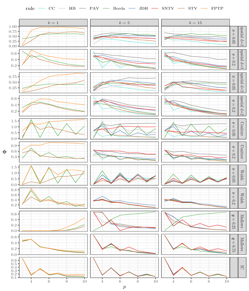
Figure 3. Spoiler susceptibility of electoral rules with respect to the normalized Penrose–Banzhaf power index.

8. Summary

We have introduced a novel approach to defining spoilers in multi-district party elections, alongside with modified probabilistic models that serve for randomly generating such elections. We compare various voting methods via simulations. The results depend strongly on a given distribution of preferences, although there are some clear patterns. An electoral system designer acting behind a veil of ignorance who is interested in maximizing spoiler resistance would do well to choose STV, CC, or Harmonic Borda, since they perform best under spatial and Conitzer models (which are most susceptible to spoilers), and under other models differences are negligible. On the other hand, for the same reason he should avoid $k$–PAV and FPTP (which is equivalent to $1$–PAV). The performance of $k$–Borda depends strongly on the degree of party clustering, while of that of Jefferson–D’Hondt – on the single peakedness of the model. Finally, single-member districts are nearly always more susceptible to spoilers than multi-member ones.

References

- Arrow [1950] K. J. Arrow. A Difficulty in the Concept of Social Welfare. Journal of Political Economy, 58(4):328–346, 1950. doi: 10.1086/256963.
- Bakker et al. [2015] R. Bakker, C. de Vries, E. Edwards, L. Hooghe, S. Jolly, G. Marks, J. Polk, J. Rovny, M. Steenbergen, and M. Vachudova. Measuring party positions in Europe: The Chapel Hill expert survey trend file, 1999–2010. Party Politics, 21(1):143–152, 2015. ISSN 1354-0688. doi: 10.1177/1354068812462931.
- Bakker et al. [2021] R. Bakker, L. Hooghe, S. Jolly, G. Marks, J. Polk, J. Rovny, M. Steenbergen, and M. Vachudova. Chapel Hill Expert Survey (CHES) Europe 1999-2019 Trend File, 2021.
- Balinski and Young [1978] Michel L. Balinski and H. Peyton Young. The Jefferson Method of Apportionment. SIAM Review, 20(2):278–284, 1978. doi: 10.1137/1020040.
- Banzhaf [1964] J.F. Banzhaf. Weighted Voting Doesn’t Work: A Mathematical Analysis. Rutgers Law Review, 19:317–343, 1964.
- Berg and Lepelley [1994] S. Berg and D. Lepelley. On Probability Models in Voting Theory. Statistica Neerlandica, 48(2):133–146, 1994. doi: 10.1111/j.1467-9574.1994.tb01438.x.
- Boehmer et al. [2021] N. Boehmer, R. Bredereck, P. Faliszewski, R. Niedermeier, and S. Szufa. Putting a compass on the map of elections. In Proceedings of IJCAI-2021, pages 59–65, 2021.
- Bordes and Tideman [1991] G. Bordes and N. Tideman. Independence of Irrelevant Alternatives in the Theory of Voting. Theory and Decision, 30(2):163–186, 1991. ISSN 1573-7187. doi: 10.1007/BF00134122.
- Börgers [2010] C. Börgers. Mathematics of Social Choice: Voting, Compensation, and Division. Society for Industrial and Applied Mathematics, Philadelphia, 2010. ISBN 978-0-89871-695-5.
- Campbell and Tullock [1965] C.D. Campbell and G. Tullock. A Measure of the Importance of Cyclical Majorities. The Economic Journal, 75(300):853–857, 1965. doi: 10.2307/2229705.
- Chamberlin and Courant [1983] J.R. Chamberlin and P.N. Courant. Representative Deliberations and Representative Decisions: Proportional Representation and the Borda Rule. American Political Science Review, 77(3):718–733, 1983. ISSN 0003-0554, 1537-5943. doi: 10.2307/1957270.
- Chevaleyre et al. [2010] Y. Chevaleyre, J. Lang, N. Maudet, and J. Monnot. Possible Winners when New Candidates Are Added: The Case of Scoring Rules. Proceedings of the AAAI, 24(1):762–767, 2010. ISSN 2374-3468.
- Conitzer [2009] V. Conitzer. Eliciting single-peaked preferences using comparison queries. Journal of Artificial Intelligence Research, 35:161–191, 2009.
- Critchlow et al. [1991] D.E. Critchlow, M.A. Fligner, and J.S. Verducci. Probability Models on Rankings. Journal of Mathematical Psychology, 35(3):294–318, 1991. ISSN 0022-2496. doi: 10.1016/0022-2496(91)90050-4.
- de Borda [1781] J.-C. de Borda. Mémoire sur les élections au scrutin. In Histoire de l’Académie Royale Des Sciences, pages 657–665. Imp. Royale, Paris, 1781.
- D’Hondt [1882] V. D’Hondt. Système Pratique et Raisonné de Représentation Proportionnelle. Libraire C. Muquardt, Bruxelles, 1882. doi: 10.3931/e-rara-39876.
- D’Hondt [1885] V. D’Hondt. Exposé Du Système Pratique de Représentation Proportionnelle. Adopté Par Le Comité de l’Association Réformiste Belge. Eug. Vanderhaeghen, Gand, 1885.
- Dubey and Shapley [1979] P. Dubey and L.S. Shapley. Mathematical Properties of the Banzhaf Power Index. Mathematics of Operations Research, 4(2):99–131, 1979. ISSN 0364-765X. doi: 10.1287/moor.4.2.99.
- Dutta et al. [2001] B. Dutta, M.O. Jackson, and M. Le Breton. Strategic Candidacy and Voting Procedures. Econometrica, 69(4):1013–1037, 2001.
- Ehlers and Weymark [2003] L. Ehlers and J.A. Weymark. Candidate Stability and Nonbinary Social Choice. Economic Theory, 22(2):233–243, 2003.
- Enelow and Hinich [1984] J.M. Enelow and M.J. Hinich. The Spatial Theory of Voting: An Introduction. Cambridge University Press, Cambridge, UK, 1984. ISBN 978-0-521-25507-3 978-0-521-27515-6.
- Eraslan and McLennan [2004] H.H. Eraslan and A. McLennan. Strategic Candidacy for Multivalued Voting Procedures. Journal of Economic Theory, 117(1):29–54, 2004.
- Erdélyi et al. [2021] G. Erdélyi, M. Neveling, C. Reger, J. Rothe, Y. Yang, and R. Zorn. Towards Completing the Puzzle: Complexity of Control by Replacing, Adding, and Deleting Candidates or Voters. Autonomous Agents and Multi-Agent Systems, 35(2):41, 2021. ISSN 1573-7454. doi: 10.1007/s10458-021-09523-9.
- Faliszewski and Rothe [2016] P. Faliszewski and J. Rothe. Control and Bribery in Voting. In A.D. Procaccia, F. Brandt, J. Lang, U. Endriss, and V. Conitzer, editors, Handbook of Computational Social Choice, pages 146–168. Cambridge University Press, Cambridge, 2016. ISBN 978-1-107-44698-4. doi: 10.1017/CBO9781107446984.008.
- Faliszewski et al. [2017] P. Faliszewski, P. Skowron, A. Slinko, and N. Talmon. Multiwinner Rules on Paths From k-Borda to Chamberlin–Courant. pages 192–198, 2017.
- Faliszewski et al. [2018a] P. Faliszewski, P. Skowron, A. Slinko, and N. Talmon. Committee Scoring Rules: Axiomatic Characterization and Hierarchy. Technical Report arXiv: 1802.06483 [cs.GT], 2018a.
- Faliszewski et al. [2018b] P. Faliszewski, S. Szufa, and N. Talmon. Optimization-Based Voting Rule Design: The Closer to Utopia the Better. In Proceedings of AAMAS-2018, pages 32–40, 2018b.
- Flis et al. [2020] J. Flis, W. Słomczyński, and D. Stolicki. Pot and Ladle: A Formula for Estimating the Distribution of Seats Under the Jefferson–D’Hondt Method. Public Choice, 182:201–227, 2020. ISSN 0048-5829, 1573-7101. doi: 10.1007/s11127-019-00680-w.
- Hare [1859] T. Hare. A Treatise on the Election of Representatives, Parliamentary and Municipal. Longman & al., London, 1859.
- Holliday and Pacuit [2021] W.H. Holliday and E. Pacuit. Split Cycle: A New Condorcet Consistent Voting Method Independent of Clones and Immune to Spoilers. Technical Report arXiv: 2004.02350 [cs.GT], 2021.
- Jefferson [1792] T. Jefferson. Opinion on Apportionment Bill. In B. Oberg and J.J. Looney, editors, Papers of Thomas Jefferson, Digital Edition. University of Virginia Press, Rotunda, Charlottesville, two thousand, eighth edition, 1792.
- Kaminski [2018] M.M. Kaminski. Spoiler Effects in Proportional Representation Systems: Evidence from Eight Polish Parliamentary Elections, 1991–2015. Public Choice, 176(3-4):441–460, 2018. doi: 10.1007/s11127-018-0565-x.
- Kendall [1938] M.G. Kendall. A New Measure of Rank Correlation. Biometrika, 30(1/2):81–93, 1938. ISSN 0006-3444. doi: 10.2307/2332226.
- Kilgour [2010] D.M. Kilgour. Approval Balloting for Multi-winner Elections. In J.-F. Laslier and M.R. Sanver, editors, Handbook on Approval Voting, Studies in Choice and Welfare, pages 105–124. Springer, Berlin, Heidelberg, 2010. ISBN 978-3-642-02839-7. doi: 10.1007/978-3-642-02839-7˙6.
- Liu et al. [2009] H. Liu, H. Feng, D. Zhu, and J. Luan. Parameterized Computational Complexity of Control Problems in Voting Systems. Theoretical Computer Science, 410:2746–53, 2009. ISSN 0304-3975. doi: 10.1016/j.tcs.2009.04.004.
- Lu and Boutilier [2014] T. Lu and C. Boutilier. Effective Sampling and Learning for Mallows Models with Pairwise-Preference Data. Journal of Machine Learning Research, 15(1):3783–3829, 2014. ISSN 1532-4435.
- Mallows [1957] C.L. Mallows. Non-Null Ranking Models. I. Biometrika, 44(1-2):114–130, 1957. ISSN 0006-3444. doi: 10.1093/biomet/44.1-2.114.
- Matsui and Matsui [2001] Y. Matsui and T. Matsui. NP-Completeness for Calculating Power Indices of Weighted Majority Games. Theoretical Computer Science, 263(1-2):305–310, 2001. ISSN 03043975. doi: 10.1016/S0304-3975(00)00251-6.
- Meir et al. [2008] R. Meir, A.D. Procaccia, J.S. Rosenschein, and A. Zohar. Complexity of Strategic Behavior in Multi-Winner Elections. Journal of Artificial Intelligence Research, 33:149–178, 2008. ISSN 1076-9757. doi: 10.1613/jair.2566.
- Merrill [1984] S. Merrill. A Comparison of Efficiency of Multicandidate Electoral Systems. American Journal of Political Science, 28(1):23–48, 1984. ISSN 00925853. doi: 10.2307/2110786.
- Neveling et al. [2020] M. Neveling, J Rothe, and R. Zorn. The Complexity of Controlling Condorcet, Fallback, and k-Veto Elections by Replacing Candidates or Voters. In H. Fernau, editor, Computer Science – Theory and Applications, Lecture Notes in Computer Science, pages 314–327, Cham, 2020. Springer. ISBN 978-3-030-50026-9. doi: 10.1007/978-3-030-50026-9˙23.
- Penrose [1946] L.S. Penrose. The Elementary Statistics of Majority Voting. Journal of the Royal Statistical Society, 109(1):53–57, 1946. doi: 10.2307/2981392.
- Polk et al. [2017] J. Polk, J. Rovny, R. Bakker, E. Edwards, L. Hooghe, S. Jolly, J. Koedam, F. Kostelka, G. Marks, G. Schumacher, M. Steenbergen, M. Vachudova, and M. Zilovic. Explaining the Salience of Anti-Elitism and Reducing Political Corruption for Political Parties in Europe with the 2014 Chapel Hill Expert Survey Data. Research & Politics, 4(1):2053168016686915, 2017. ISSN 2053-1680. doi: 10.1177/2053168016686915.
- Prasad and Kelly [1990] K. Prasad and J.S. Kelly. NP-Completeness of Some Problems Concerning Voting Games. International Journal of Game Theory, 19(1):1–9, 1990. ISSN 0020-7276, 1432-1270. doi: 10.1007/BF01753703.
- Pukelsheim [2017] F. Pukelsheim. Proportional Representation: Apportionment Methods and Their Applications. Second Edition. Springer International, Cham–Heidelberg, 2017. ISBN 978-3-319-64706-7. doi: 10.1007/978-3-319-64707-4.
- Ray [1973] P. Ray. Independence of Irrelevant Alternatives. Econometrica, 41(5):987–991, 1973. ISSN 0012-9682. doi: 10.2307/1913820.
- Regenwetter et al. [2006] M. Regenwetter, B. Grofman, I. Tsetlin, and A.A.J. Marley. Behavioral Social Choice: Probabilistic Models, Statistical Inference, and Applications. Cambridge University Press, Cambridge, UK, 2006. ISBN 0-521-53666-9.
- Rodríguez-Álvarez [2006] C. Rodríguez-Álvarez. Candidate Stability and Voting Correspondences. Social Choice and Welfare, 27(3):545–570, 2006. ISSN 0176-1714.
- Shapley and Shubik [1954] L. Shapley and M. Shubik. A Method for Evaluating the Distribution of Power in a Committee System. American Political Science Review, 48(3):787–792, 1954. ISSN 0003-0554. doi: 10.2307/1951053.
- Szufa et al. [2020] S. Szufa, P. Faliszewski, P. Skowron, A. Slinko, and N. Talmon. Drawing a Map of Elections in the Space of Statistical Cultures. In Proceedings of AAMAS-2020, pages 1341–1349. 2020. ISBN 978-1-4503-7518-4.
- Thiele [1895] T.N. Thiele. Om Flerfoldsvalg. Oversigt over det Kongelige Danske Videnskabernes Selskabs Forhandlinger, 1894:415–441, 1895.
- Tideman [1987] T.N. Tideman. Independence of Clones as a Criterion for Voting Rules. Social Choice and Welfare, 4(3):185–206, 1987. ISSN 1432-217X. doi: 10.1007/BF00433944.
- Tideman and Plassmann [2012] T.N. Tideman and F. Plassmann. Modeling the Outcomes of Vote-Casting in Actual Elections. In D.S. Felsenthal and M. Machover, editors, Electoral Systems. Paradoxes, Assumptions, and Procedures, pages 217–251. Springer, Berlin–Heidelberg, 2012. doi: 10.1007/978-3-642-20441-8˙9.
- Tideman and Richardson [2000] T.N. Tideman and D. Richardson. Better Voting Methods Through Technology: The Refinement-Manageability Trade-Off in the Single Transferable Vote. Public Choice, 103(1):13–34, 2000. ISSN 1573-7101. doi: 10.1023/A:1005082925477.
- Walsh [2015] T. Walsh. Generating single peaked votes. Technical Report arXiv:1503.02766 [cs.GT], arXiv.org, March 2015.