On an Asymptotic Criterion for Blockchain Design:
The Asynchronous Composition Model

Abstract

Inspired by blockchains, we introduce a dynamically growing model of rooted Directed Acyclic Graphs (DAGs) referred to as the asynchronous composition model, subject to i.i.d. random delays $(\xi_{t})_{t}$ with finite mean. The new vertex at time $t$ is connected to vertices chosen from the graph $G_{(t-\xi_{t})_{+}}$ according to a construction function $f$ and the graph is updated by taking union with the graph $G_{t-1}$. This process corresponds to adding new blocks in a blockchain, where the delays arise due to network communication. The main question of interest is the end structure of the asynchronous limit of the graph sequence as time increases to infinity.

We consider the following construction functions of interest, a) Nakamoto construction $f_{\mathrm{Nak}}$, in which a vertex is uniformly selected from those furthest from the root, resulting in a tree, and b) mixture of construction functions $(f_{k})_{1\leqslant k\leqslant\infty}$, where in $f_{k}$ a random set of $k$ leaves (all if there are less than $k$ in total) is chosen without replacement.

The main idea behind the analysis is decoupling the time-delay process from the DAG process and constructing an appropriate regenerative structure in the time-delay process giving rise to Markovian behavior for a functional of the DAG process. We establish that the asynchronous limits for $f_{\mathrm{Nak}},(f_{k})_{k\geqslant 2}$, and any non-trivial mixture $f$ are one-ended, while the asynchronous limit for $f_{1}$ has infinitely many ends, almost surely. We also study fundamental growth properties of the longest path for the sequence of graphs for $f_{\mathrm{Nak}}$. In addition, we prove a phase transition on the (time and sample-path dependent) probability of choosing $f_{1}$ such that the asynchronous limit either has one or infinitely many ends. Finally, we show that the construction $f_{\infty}$ is an appropriate limit of the $(f_{k})_{k}$.

and

1 Introduction

In this article, we introduce a novel model for dynamically growing directed graphs, hereafter referred to as the asynchronous composition model. Mainly inspired by blockchains, this model may also be of independent interest as a time-indexed random graph process outside the blockchain context. We also use an integer-valued asynchronous recursion to analyze the growth rate of one such asynchronous composition related to the Bitcoin system; this corresponds to asynchronous composition in a more general setting outside of random graph growth processes. The class of asynchronous recursions introduced in this paper is a new class of max-type distributional recursions whose analysis does not follow the techniques in the survey paper [2]. The analysis of asynchronous recursions may also be of independent interest.

Let $\mathcal{B}_{*}$ denote the space of all rooted, finite, and connected directly acyclic graphs (or DAGs) with each vertex marked with a non-negative integer. Let $\boldsymbol{\xi}:=(\xi_{t})_{t\geqslant 1}$ be a sequence of non-negative integers. We interpret $\boldsymbol{\xi}$ as the time delay process: the value of $\xi_{t}\geqslant 1$ is the delay seen by the process at time $t$, including the passage of a single time step. We proceed by composing the function $f$, but with asynchrony arising from the delay dynamics. Here, we use the word asynchronous to mean that the sequence of delays $\boldsymbol{\xi}$ is not identically the constant one; otherwise, we use the word synchronous. This terminology is based on the broader area of distributed systems and explains the model’s name. Let $\boldsymbol{\theta}:=(\theta_{t})_{t\geqslant 1}$ be a sequence of real numbers in $[0,1]$; this sequence drives the graph dynamics at any given time step.

We assume that the sequence $\boldsymbol{\xi}$ are i.i.d. $\mathds{N}$-valued random variables and $\boldsymbol{\theta}$ are i.i.d. U$(0,1)$ random variables independent of $\boldsymbol{\xi}$. Thus, our process is driven by two sources of randomness: the sequence $\boldsymbol{\xi}$ drives the delay, and the sequence $\boldsymbol{\theta}$ provides a source of edge-randomness for each time step. We now formally define the model.

Definition 1.1 (Asynchronous Composition Model).

The asynchronous composition model (ACM) with construction function $f$ evolves in discrete time as follows:

• At time $t=0$, we are given a finite DAG, $G_{0}=(V_{0},E_{0})\in\mathcal{B}_{*}$, such that all vertices in $G_{0}$ are marked $0$.

• At each time $t\geqslant 1$, the DAG $G_{t}:=(V_{t},E_{t})$ is determined as follows:

  $$V_{t}=V_{t-1}\cup\{t\},\quad E_{t}=E_{t-1}\cup\{(t,v)\mid v\in f(G_{(t-\xi_{t})_{+}},\theta_{t})\},$$

  where $f:(G,u)\mapsto 2^{V(G)}$ is given and $x_{+}:=\max\{x,0\}$. For simplicity of notation, we write

  $$G_{t}:=G_{t}(f)=G_{t-1}\cup f(G_{(t-\xi_{t})_{+}},\theta_{t})\text{ for }t\geqslant 1.$$ (1.1)

• All vertices are marked by the time at which they are created. We refer to the vertex of mark $i\geqslant 1$ as the $i$-th vertex or as vertex $i$.

Throughout this paper, we say the vertex at time $t$ connects to each vertex given by the function $f(G_{(t-\xi_{t})_{+}},\theta_{t})$.

Intuitively, the function $f$ in Definition 1.1 provides a random set of vertices to which the new vertex will connect. Any such function $f$ can be considered as a construction function for a blockchain system, which determines how a new block is attached to a blockchain. In this article, we will consider $f$ such that $f(G,\cdot)$ is a random subset of the leaf set, i.e., set of vertices with in-degree zero. In Section 1.2, we discuss the relevance of this model to blockchain systems in detail.

In the blockchain context, we discuss the importance of one-endedness in the temporal limit of $G_{t}$, both with and without delays. This problem corresponds to determining which construction functions $f$ are such that the temporal limit of $G_{t}$ is one-ended in both synchronous and asynchronous operations. The definition of a graph limit is made precise in Section 2.3. Our primary focus is a class of construction functions based on the Iota [21] protocol; this is one of the more widely used protocols for which one-endedness has not yet been established. The Iota protocol uses a construction function that behaves as follows: given a DAG $G$, a pair of vertices is chosen through some (unspecified in [21]) measure. The new vertex connects to both vertices in this pair. In this paper, we assume that this measure is uniform for simplicity. The uniformity assumption is also made in King’s analysis of the Iota protocol [19].

For the rest of this paper, we assume that $\operatorname{\mathds{E}}\xi<\infty$; more specifically, for technical reasons our proofs require the assumption that $\operatorname{\mathds{E}}\xi^{1+\delta}<\infty$ for some $\delta>0$. When $\operatorname{\mathds{E}}\xi=\infty$, using the fact that $\operatorname{\mathds{E}}\xi=\sum_{t\geqslant 1}\operatorname{\mathds{P}}(\xi\geqslant t)$, one can easily see that the degree of the root vertex diverges to infinity almost surely; hence the limiting graph will not be locally finite. Thus the limits considered in this paper do not exist when $\operatorname{\mathds{E}}\xi=\infty$. Moreover, it will be clear that this situation is undesirable in the blockchain context. Even in the $\operatorname{\mathds{E}}\xi<\infty$ case, the two cases $\operatorname{\mathds{P}}(\xi=1)>0$ and $\operatorname{\mathds{P}}(\xi=1)=0$ behave differently. We discuss this further in Section 1.1. Also, not every function with a one-ended synchronous limit has a one-ended asynchronous limit; this presents a fundamental challenge to the analysis.

Assume that $f_{\operatorname{{Nak}}}$ is the Nakamoto construction function, where a vertex is chosen uniformly from those at the maximum hop distance from the root. For $k\geqslant 1$, we denote by $f_{k}$ the construction function, which chooses a set of $k$ leaves uniformly at random from the set of $k$-tuples of leaves. If less than $k$ leaves for $k\geqslant 2$, we chose all leaves in the graph. The function $f_{\infty}$ is such that all leaves are chosen in the graph. Our main results are summarized as follows. Detailed statements are given in Section 2.5.

• Theorem 2.15 – For the Nakamoto construction function $f_{\operatorname{{Nak}}}$, we prove a closed-form expression for the growth rate of the longest path to the root in $G_{t}$. This expression corresponds precisely to the fraction of confirmed vertices in the asynchronous limit. This expression for the growth rate is a universal upper bound on the growth rate of the same quantity for any construction function.

• Theorem 2.17 and 2.18 – The synchronous limit of $f_{1}$ has as many ends as leaves in $G_{0}$. We show that the asynchronous limit of $f_{1}$ has infinitely many ends almost surely, even starting from a single vertex at time zero. In particular, the number of leaves in $G_{t}(f_{1})$ grows as $\Theta(\sqrt{t})$. However, for any mixture $f$ of the $(f_{k})_{k}$ such that $\operatorname{\mathds{P}}(f=f_{1})<1$, we show that both the synchronous and asynchronous limits of $G_{t}(f)$ are almost surely one-ended. See figure 1 below for two simulated graphs with $f=f_{1}$ and $f=f_{2}$, respectively.

• Theorem 2.19 – Finally, we consider the time-varying construction functions $(f_{t})_{t}$, which is a mixture of the $(f_{k})_{k}$ for every $t$. We identify (up to order) the state-based threshold for $\operatorname{\mathds{P}}(f_{t}=f_{1})$ above which the asynchronous limit is one-ended. We also prove that the graph process related to the function $f_{\infty}$ is an appropriate limit of the processes related to the $(f_{k})_{k}$, as expected.

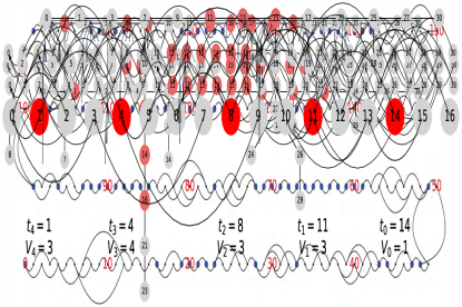
Figure 1: Sample $G_{1000}$ with $f_{1}$ and $f_{2}$, respectively, with Geometric(3/4) delay distribution. Graphs were drawn using Kamada-Kawai spring layout from python networkx module.

The crucial step in our analysis is decoupling the delay dynamics and the graph dynamics built on top. We define the notion of time-delay graph in Section 1.1 below. Moreover, recurrence of specific local graph structure will imply one-endedness.

When $\operatorname{\mathds{P}}(\xi=1)>0$, it suffices to know the number of leaves at the regeneration times. Indeed it will be shown in Lemma 2.12 that if there are infinitely many regeneration times where the new vertex connects to a unique single leaf, the limit graph is one-ended. When $\operatorname{\mathds{P}}(\xi=1)\geqslant 0$, we use a more complicated state space at the regeneration intervals of length $r:=\min\{k\geqslant 1\mid\operatorname{\mathds{P}}(\xi=k)>0\}$, which reduces to the previous state space when $\operatorname{\mathds{P}}(\xi=1)>0$. We consider a specific finite graph structure over a sequence of consecutive regeneration intervals, which implies that all initially present leaves are confirmed. This structure can easily be seen when $\xi=r$ a.s. This regenerative DAG structure, for $r=3$, is shown pictorially in Figure 2. This state-space is explicitly described in Section 6.4.2.

            

Figure 2: Graph representation (in two ways) of regenerative block structure for the DAG process for the function $f_{2}$ when $r=3$. Vertices before label $1$ represent the graph before the beginning of the event being depicted. Here, vertices $1,2,3$ are confirmed in the limit, when the time interval $[10,12]$ is a regeneration interval.

1.1 Time-Delay Graph

Given the delay sequence $\boldsymbol{\xi}=(\xi_{t})_{t\geqslant 0}$, we construct a time-delay graph on the vertex set $\mathds{Z}_{+}$ as follows. Each vertex $i\geqslant 1$ connects to vertex $(i-\xi_{i})_{+}$; and vertex $0$ has out-degree $0$.

The time-delay graph is always a tree. When the period $d$ of the support of $\xi$ is greater than $1$, this tree has $d$ ends. Otherwise, it is one-ended. Note that the in-degree of a vertex in the time-delay graph depends on future times, so stopping time-based arguments are not applicable. However, when $\operatorname{\mathds{E}}\xi<\infty$ and $\operatorname{\mathds{P}}(\xi=1)>0$, we show in Corollary 3.2 that there are infinitely many “regeneration times”; these times correspond to “synchronization moments” in a more descriptive network model such as the one in [16]. Regeneration time corresponds to all vertices $t_{0}$ in the time-delay graph such that there are no edges between vertices to the left and the right of $t_{0}$. See figure 3 for a simulated time-delay graph.

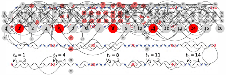
Figure 3: A sample time-delay graph, with linear and tree representation, respectively, with Geometric(1/2) delay. The regeneration times are given by red vertices. The third graph is ACM with Nakamoto construction function built with the given delay process (red vertices represent anchor vertices).

We show that the graph process at the regeneration times defines a Markov chain on $\mathcal{B}_{*}$. When this graph has its edges reversed, the regeneration times correspond to renewals or vertices such that any infinite path leading away from $0$ passes through said vertices. This process with the reversed edges is studied more carefully by Baccelli and Sodre [5].

When $\operatorname{\mathds{P}}(\xi=1)=0$ with $\operatorname{\mathds{E}}\xi<\infty$, we do not have the existence of any regeneration times; however a similar analysis can be carried out with “regeneration intervals” of length $r:=\min\{i\mid\operatorname{\mathds{P}}(\xi=i)>0\}$. See figure 4 for a simulated time-delay graph with $r=2$.

Figure 4: A sample time-delay graph, with linear and tree representation, respectively, with 1+Geometric(1/2) delay. The regeneration intervals are given by red vertices. The third graph is ACM with $f_{2}$ construction function built with the given delay process (red vertices represent regenerative block structure for the DAG process).

1.2 Relevance to Blockchain

Blockchain protocols are a new class of network consensus protocols that were introduced by Nakamoto’s Bitcoin whitepaper [20]. Each node in the network creates new data, called blocks, and the nodes exchange these blocks through pairwise communication [16, 14, 15, 13] with the goal of network-wide synchronization. This communication is subject to potentially unbounded delay.

The blocks correspond to vertices in a DAG; each vertex has an out-degree at least one. The choice of the outgoing edges is a form of distributed trust; see [20, 16, 9] for more details. A vertex, trusted by all network nodes, is called a confirmed vertex. Under this terminology, we can express the blockchain problem as follows.

Given a DAG, which vertices are confirmed?

We defer our comments about confirmed vertices until the end of this subsection for organizational clarity.

When $\operatorname{\mathds{E}}\xi=\infty$, infinitely many vertices will connect to the vertices with mark $0$. In this situation, the distributed trust dynamics can be interpreted as a system that makes no progress: for example, if there are only $N$ nodes in the network, this situation corresponds to nodes verifying some information more than once. Thus, the local finiteness of the limit is a crucial consideration for blockchain design.

Due to communication delay, at any time $t$, nodes may not be synchronized; thus, the problem of achieving consensus on the set of confirmed vertices is a complex issue. Recent work (see [16]) shows that the asymptotic property of almost sure one-endedness of the blockchain DAG allows nodes to agree on an infinite subset of confirmed vertices in the limit as time $t\to\infty$. Imprecisely, one-endedness is a topological property of an infinite graph, implying “growth to infinity only in one direction.” This concept is closely related to ends in a general topological space [11]. See Section 2.3 for a rigorous definition.

Thus, any effectively designed blockchain protocol achieves eventual one-endedness in synchronous and asynchronous operations, even though no real-world network can be genuinely synchronous. This paper provides a general framework to analyze the asynchronous dynamics of synchronously defined blockchain protocols. Specifically, we abstract the network synchronization problem to the behavior of the random variables $\boldsymbol{\xi}$ and the attachment of new vertices to the blockchain DAG to the construction function $f$ to isolate the DAG dynamics. To our knowledge, this is the first paper to isolate the DAG dynamics of general blockchain protocols. While King [19] does study a related model that works only studies a restricted functional of the graph process and not the process itself.

Many practical considerations, such as the security of blockchain implementation, inherently depend on successful consensus dynamics and thus the guarantee of eventual one-endedness. We hope that through a unified study of blockchain consensus dynamics, such considerations can also be unified, rather than studied on a case-by-case basis, as is presently the state-of-the-art (e.g. [9, 22]).

1.2.1 Confirmed Vertices

In Nakamoto’s original Bitcoin whitepaper [20] and subsequent work on blockchain security such as [9, 22], the definition of a “confirmed” vertex is at least the $k$–th vertex on the path from (one of) the furthest leaf (leaves) to the root. This definition holds only for the construction function given in Nakamoto’s protocol.

There are several problems with this definition, many of which arise even in Nakamoto’s Bitcoin protocol analysis. First, this definition refers to vertices as confirmed, even if they may eventually be “unconfirmed” due to the behavior of network delays (even without an adversarial agent). Second, even if defined for a particular construction function, the definition of a confirmed block should be invariant to the delay model. We note that network instability (e.g., in the sense of instability of the Markov models studied by [16]; the same concept is a key question in the analysis of queueing networks [6]) may lead to a limit graph with more than one end. In this case, the previous notion of a confirmed block includes vertices that should not be confirmed (and the set of “confirmed” vertices is not monotone).

A similar situation also arises in this paper where the support of the delays $\boldsymbol{\xi}$ does not include $1$, despite the existence of regeneration intervals with finite expected inter-regeneration lengths. The main difficulty with this definition is that confirmation and one-endedness are properties of limits of the process (thus, of an infinite graph) which cannot be inferred from the pre-limit process. Moreover, this definition does not readily generalize to other constructions.

Instead, we use the asymptotic definition of a “confirmed vertex” given in Gopalan et al. [16]: a vertex is confirmed if all but finitely many future vertices reference it. This definition resolves all of the issues mentioned above. Furthermore, an asymptotic approach to studying confirmation in such systems is more mathematically tractable.

1.3 Related Work

The time-delay model in our paper is closely related to the work of Baccelli and Sodre [5]. In their model, at each time $t$ (indexed by $\mathds{Z}$), a new vertex marked $t$ is added to a tree with a directed edge to the vertex $t+\nu_{t}$, where the $(\nu_{t})_{t}$ are i.i.d. One can think of this graph as having edges pointing to the future. Note that when $\operatorname{\mathds{E}}\nu_{1}<\infty$, this process, with reversed edges pointing to the past, uniquely determines the sequence $\boldsymbol{\xi}$ in our paper. We called this new graph with reversed edges the time-delay graph. Their future edge direction allows them to use stopping time methods to determine a renewal structure and study the unimodularity of the resulting tree. In the delay graph process, the regeneration times are not stopping times, which adds additional difficulty to the analysis. Moreover, the asynchronous composition model constructs graphs and trees with a more complicated structure, and we cannot immediately use their results to analyze our limiting graphs. The caveat to a more complicated analysis is that the time-delay graph as specified in our model more realistically captures delay dynamics in an internet network system, where different nodes in the network will learn of a piece of data at different times. This is achieved with our time-delay graph, whereas with edges pointing to the future, all nodes learn of any given data instantly. In Section 2.6, we mention a generalization of the ACM model combining both forward and backward delays.

In our model, recurrence of “regeneration intervals” in the time-delay graph plays a crucial role in defining a Markov chain for the actual DAG dynamics. Regenerative analysis for graphs based on the one-dimensional integer lattice is already present in the random growth model literature. For example, in the long-range last–passage percolation on the real line [12], long-range first–passage percolation in the one dimension case [8], among others.

King [19] studies the function $f_{2}$, which is in the main class of functions of interest in this paper. As with the work of Baccelli and Sodre [5], the delay graph in [19] has edges pointing to the future; but in [19] the delays are a fixed constant. This particular case is the same as setting $\xi_{t}=k$ in our model for some fixed $k$, for all times $t$. The author proves the existence of a stationary distribution for the number of leaves in the limit graph for this function. In the particular case of that paper, we note that this result implies one-endedness of the limit graph, but the author does not consider the topology of the limit graph. In this paper, along with our emphasis on the topological properties of the limit graph, we consider a more general process with random delays.

As with many stochastic growth models, our analysis is concerned with studying limiting behavior in space and time. We briefly contrast the model in this paper with those in other well-studied classes of problems, such as preferential attachment model, percolation, and unimodular random graphs. Our recursion in equation (1.1) closely resembles the dynamics of preferential attachment when the delays $\boldsymbol{\xi}$ are equal to one. However, we note that the model with random delays is not well-studied, and the analysis requires different techniques.

In addition, unlike in preferential attachment and percolation, where the goal is to study the local graphical structure and the number of connected components, we study the (topological) end structure of the limiting graph, which cannot be directly inferred from the local properties. Both the delay and the study of the end structure are motivated by the blockchain application [16]. Finally, recent work on unimodular random graphs [3] studies the end structure of stochastic growth processes on a class of trees. The models in those papers do not directly incorporate delays, and thus, the analysis does not apply to our problem. Also, our problem statement and primary analysis are concerned with DAGs and are not restricted to trees.

Analysis of asymptotic properties of limiting infinite graphs has also been used to study convergence properties for opinion dynamics in social networks [1]. In this paper, the main question about the limit graph is whether every finite subgraph has finite in-degree. This condition is related to but not necessarily equivalent to the end structure we study in this paper. However, as discussed above, the limiting end structure is of key importance in the blockchain context.

1.4 Organization of the Paper

The paper is structured as follows. In Section 2, we state our main results and the requisite definitions which we use in this paper. We also describe our notations there. In Section 3, we discuss the regenerative behavior of the time-delay graph. We discuss some examples of asynchronous composition in Section 4. In Sections 5 and 6, we prove the statements concerning the regenerative behavior in the time-delay graph and our main results, respectively. Finally, in Section 7, we discuss our results and some directions for future work.

2 Definitions and Main Result

For the rest of this paper, the term graph always refers to a directed acyclic graph (DAG).

2.1 Assumptions

We use $\xi$ and $\theta$ to refer random variables distributed identically to $\xi_{1}$ and $\theta_{1}$, respectively, for clarity of presentation. We will assume the following throughout the rest of the article:

• $\operatorname{\mathds{P}}(\xi\geqslant 1)=1$ and $\operatorname{\mathds{E}}\xi^{1+\delta}<\infty$ for some $\delta>0$,

• $\theta\sim\text{Uniform}([0,1])$.

2.2 Notations

For the rest of the article, we will follow the notations enumerated below for easy reference.

• For any real numbers $x,y$, we denote:

  $$x\wedge y=\min(x,y);\ x\vee y=\max(x,y);\ x_{+}=x\wedge 0;\ x_{-}=(-x)\wedge 0.$$

• For a graph $G=(V,E)$, we use the notation $u\to v$ if there is a directed path from the vertex $u$ to the vertex $v$ in $G$. It is clear from the definition of the asynchronous composition model that for any vertex $u$, $u\not\to u$.

• $\mathcal{B}_{\star}(\overline{\mathcal{B}}_{\star})$ denote the set of all rooted, connected DAGs with finitely (infinitely) many vertices.

• $\boldsymbol{\xi}:=(\xi_{t})_{t\geqslant 1}$ is the i.i.d. driving sequence of delays. We use the notation $\boldsymbol{\xi}_{i}^{j}:=(\xi_{i},\xi_{i+1},\ldots$, $\xi_{j})$ for $1\leqslant i\leqslant j\leqslant\infty$.

• $\boldsymbol{\theta}:=(\theta_{t})_{t\geqslant 1}$ is the i.i.d. driving sequence for the randomness at any instant. We use the notation $\boldsymbol{\theta}_{i}^{j}:=(\theta_{i},\theta_{i+1},\ldots,\theta_{j})$ for $1\leqslant i\leqslant j\leqslant\infty$ and

  $$f^{t}(G;\boldsymbol{\theta}_{1}^{t},\boldsymbol{\xi}_{1}^{t}):=G_{t}\text{ where }G_{t}=G_{t-1}\cup f(G_{(t-\xi_{t})_{+}},\theta_{t}),\quad t=1,2,\ldots$$

  for any $G\in\mathcal{B}_{*}$.

• $\mathcal{F}_{t}:=\sigma(\xi_{1},\ldots,\xi_{t},\theta_{1},\ldots,\theta_{t})$ is the $\sigma$-algebra generated by the trajectories up to time $t$.

• If needed, we will use the notation $G_{t}(f)$ instead of $G_{t}$ to emphasize that the asynchronous composition is with respect to the function $f$.

• We denote by $(\tau_{k})_{k\geqslant 1}$ the sequence of regeneration times as given in Definition 2.13, with $\tau_{1}\geqslant 0$ being the first regeneration time after time $0$. We denote by $(\tilde{\tau}_{k})_{k\geqslant 0}$ the sequence of instants at the beginning of regeneration intervals, as given in Definition 2.14

• We denote by $\gamma_{i}:=\tau_{i+1}-\tau_{i}$ and $\tilde{\gamma}_{i}:=\tilde{\tau}_{i+1}-\tilde{\tau}_{i}$ for $i\geqslant 1$.

• We will use the calligraphic letter $\mathcal{A}_{t}$ to denote a set at time $t$, and the corresponding roman letter $A_{t}$ to denote the cardinality of that set. We will use the corresponding notation $\hat{\mathcal{A}}_{k}=\mathcal{A}_{\tau_{k}}$ to denote the same set at the $k$-th regeneration time, along with the corresponding notation $\hat{A}_{k}$. We also use the notation $\tilde{\mathcal{A}}_{k}=\mathcal{A}_{\tilde{\tau}_{k}}$ to denote the same set at the first instant of the $k$-th regeneration interval, along with the corresponding notation $\hat{\tilde{A}}_{k}$.

• We introduce the following:

  • $\mathcal{L}(G)$ denotes the set of leaves (nodes with out-degree one) in the graph $G$, and $L(G)$ its size.

  • $\mathcal{I}_{t,s}:=\mathcal{L}(G_{s})\cap\mathcal{L}(G_{t})^{c}\text{ for }t\geqslant s,$ is the set of leaves at time $s$ which are not leaves at time $t$. $I_{t,s}$ is the size of $\mathcal{I}_{t,s}$.

• We will use the shorthand $\mathcal{L}_{t},L_{t}$ for $\mathcal{L}(G_{t}),L(G_{t})$, respectively. Similarly, we will use $\hat{\mathcal{L}}_{k},\hat{L}_{k}$, $\tilde{\mathcal{L}}_{k}$, $\tilde{L}_{k}$ for $\mathcal{L}(G_{\tau_{k}}),L(G_{\tau_{k}}),\mathcal{L}(G_{\tilde{\tau}_{k}}),L(G_{\tilde{\tau}_{k}})$, respectively.

2.3 Infinite Graphs

A graph $G=(V,E)$ is infinite if $V$ is infinite. An infinite graph $G$ is locally finite if all vertices $v\in V$ have finite degree.

We define $\overline{\mathcal{B}}_{\star}$ as the set of all rooted, locally finite, connected DAGs. Clearly, $\mathcal{B}_{\star}\subseteq\overline{\mathcal{B}}_{\star}$. However, the notion of endedness is only relevant for infinite graphs. We make the idea precise below. We define a ray as a semi-infinite directed path in an infinite graph $G\in\overline{\mathcal{B}}_{\star}$.

Definition 2.1 (See [17]).

Two infinite rays $p_{1}$ and $p_{2}$ in $G$ are equivalent if there exists a third infinite ray $p_{3}$ such that $|p_{1}\cap p_{3}|=|p_{2}\cap p_{3}|=\infty$, where the intersection is taken over vertices.

Lemma 2.2.

Two infinite rays $p_{1}$ and $p_{2}$ in $G$ are equivalent iff for any finite subgraph $S$ containing the root which only has a single component, the following holds: for any vertices $v_{1}\in G\setminus S$ and $v_{2}\in G\setminus S$ are on $p_{1}$ and $p_{2}$, respectively, there exists a vertex $v_{3}\in G\setminus S$ such that there is a directed path from $v_{3}$ to $v_{1}$ and a directed path from $v_{3}$ to $v_{2}$.

Proof of the above lemma follows easily from standard arguments (see [10]). Being equivalent defines an equivalence relation on the set of infinite rays in $G$. Note that Definition 2.2 is analogous to constructing ends in a general topological space by using the compact-open topology.

Definition 2.3 (See [17]).

The graph $G$ is $n$-ended if the equivalence relation in Definition 2.1 separates infinite rays of $G$ into $n$ equivalence classes; each class is called an end. If there is only a single equivalence class, $G$ is one-ended. If there are no infinite rays, $G$ has $0$ ends.

Observe that the definition of ends can be extended such that any finite graph has $0$ ends. Moreover, due to König’s Lemma, any locally finite infinite graph has at least one end. From this definition, it is clear that the number of ends in an infinite graph cannot be inferred from the properties of any finite subgraph.

We endow $\overline{\mathcal{B}}_{\star}$ with the metric $d_{*}$, defined as follows.

Definition 2.4 ([3, Chapter 2]).

The function

$$d_{*}(G_{1},G_{2}):=\frac{1}{1+s}$$

where $s$ is the supremum of all integers such that the $s$–balls w.r.t. the hop distance centered at the roots of $G_{1}$ and $G_{2}$ agree, is a metric on $\overline{\mathcal{B}}_{\star}$.

It is easily checked (see [3]) that $\overline{\mathcal{B}}_{\star}$ is a complete metric space. All limits in this paper are in $\overline{\mathcal{B}}_{\star}$. For the rest of this paper, we will denote by $G_{0}$ the graph consisting of a single root vertex marked $0$ and no edges.

Definition 2.5.

The synchronous limit is given by

$$f^{\infty}(G_{0};\boldsymbol{\theta},\boldsymbol{1}):=\lim_{n\to\infty}f^{n}(G_{0};\boldsymbol{\theta}_{1}^{n},\boldsymbol{1})$$

where the limit is w.r.t. the $d_{*}$ metric.

For all functions considered in this paper, the existence of the synchronous limit is immediate, and we omit proofs for brevity.

Definition 2.6.

The asynchronous limit is given by

$$G_{\infty}(f):=\lim_{t\to\infty}G_{t}(f)=\lim_{t\to\infty}f^{t}(G_{0},\boldsymbol{\theta}_{1}^{t},\boldsymbol{\xi}_{1}^{t}),$$

where the limit is w.r.t. the $d_{*}$ metric.

Observe that the synchronous limit is the particular case of the asynchronous limit when $\xi_{t}\equiv 1$ for all $t\geqslant 1$.

Definition 2.7.

The function $f$ is $k$-ended if $f^{\infty}(G;\boldsymbol{\theta}^{\infty},\boldsymbol{1})$ is $k$-ended for any finite $G\in\mathcal{B}_{\star}$.

2.3.1 Infinite Graphs and Blockchain

A vertex $v$ in the (synchronous or asynchronous) limit of the function $f$ is confirmed if $w\to v$ for all but finitely many $w>v$. We state a lemma from [16] which identifies crucial properties of limiting blockchain graphs. In the interest of self-containedness, we include proof of this lemma.

Lemma 2.8 ([16, Lemmas 3.4 and 3.5]).

If a locally finite infinite graph $G$ is one-ended, then it has infinitely many confirmed vertices. Conversely, if $G$ has infinitely many confirmed vertices, then there is a one-ended subgraph of $G$ which contains all of the confirmed vertices.

Proof.

Suppose that $G$ is one-ended. Fix any infinite ray $p_{1}$; we will show that each vertex contained in $p_{1}$ is confirmed. For any other infinite ray $p_{2}$, we have a ray $p_{3}$ which intersects both $p_{1}$ and $p_{2}$ infinitely often. This implies that for any vertex $v$ in $p_{1}$, all but finitely many vertices in $p_{2}$ have a path to $v$. This part of the result then follows since $G$ is locally finite.

Next, suppose that $G$ has infinitely many confirmed vertices and denote by $\hat{G}$ the subgraph of the confirmed vertices. The result follows immediately from Definition 2.2. $\blacksquare$

We note that, a spanning tree for a graph $G$ is a subgraph $G^{\prime}=(V,E^{\prime})$, where $E^{\prime}\subseteq E$, the root in $G^{\prime}$ is the same as the root in $G$, and each (non-root) vertex in $G^{\prime}$ has a unique path to the root. We add the following easy corollary, which is a new result:

Corollary 2.9.

A locally finite infinite graph $G$ has infinitely many confirmed vertices iff it has a one-ended spanning tree.

In practice, it is far easier to check the one-endedness of a graph than to establish the existence of a one-ended spanning tree. So we do not use the corollary even if it expresses a tighter condition for the existence of infinitely many confirmed vertices. It follows from Lemma 2.8 that a critical question related to the design of blockchain systems is the determination of which one-ended functions have one-ended asynchronous limits.

2.3.2 Some Technical Lemmas

The following technical lemmas are helpful in our analysis, and we put them here to simplify the presentation later in the paper.

Lemma 2.10.

Let $(T_{t})_{t}$ be a sequence of finite trees with $T_{t}\subseteq T_{t+1}$ for all $t\geqslant 0$. Suppose the number of leaves is non-decreasing in $t$ and diverges to infinity, and that any leaf in $T_{t}$ is such that for some $s>t$, that leaf is not a leaf in $T_{s}$. If $T:=\lim_{t\to\infty}T_{t}$ exists in $\overline{\mathcal{B}}_{\star}$, then $T$ has infinitely many ends.

Proof.

Fix any graph $T_{t}$. Any leaf in $T_{t}$ is part of an infinite path in $T$. Thus, if there are $k$ leaves in $T_{t}$, then $T$ has at least $k$ ends. The result follows since the number of leaves in $T_{t}$ tends to infinity. $\blacksquare$

Lemma 2.11.

Let $T\in\mathcal{B}_{\star}$ be an infinite tree. $T$ is one-ended iff it has infinitely many confirmed vertices.

Proof.

If $T$ is one-ended, then it has infinitely many confirmed vertices by Lemma 2.8. Suppose $T$ has infinitely many confirmed vertices. Since $T$ is a tree, there exists an infinite path $p$ consisting of confirmed vertices. However, since $T$ is a tree, all infinite paths must intersect $p$ infinitely often. $\blacksquare$

From the definition of one-endedness, it follows easily that for an infinite graph $G$, $G$ is one-ended iff any two rays are equivalent.

Lemma 2.12.

Let $G\in\mathcal{B}_{\star}$ be an infinite graph. Suppose that there is an infinite sequence of vertices $(v_{i})_{i}$ such that any infinite path passes through $v_{i}$ for all $i$. Then $G$ is one-ended.

Proof.

In this case, all rays are clearly equivalent. The result follows from the definition. $\blacksquare$

In Lemma 2.12, the vertices in the sequence $(v_{i})_{i}$ can be thought of as anchor vertices.

2.4 Definitions for the Delay Process

For the rest of this paper, we denote by

$$r:=\min_{n\in\mathds{N}}\{n:\operatorname{\mathds{P}}(\xi=n)>0\}$$ (2.1)

the minimal point in the support of $\xi$. The following definitions provide an important structural framework for our analysis.

Definition 2.13.

An integer $t\geqslant 0$ is a regeneration time for the delay sequence $(\xi_{s})_{s\geqslant 0}$ if $\xi_{t}=1$ and $\xi_{t+s}\leqslant s$ for all $s\geqslant 1$.

Note that, $t$ is a regeneration time iff $1\leqslant\xi_{t+s}\leqslant s\vee 1$ for all $s\geqslant 0$. For regeneration time to exist, clearly we need $\operatorname{\mathds{P}}(\xi=1)>0$ or $r=1$. In the general case, we define “regeneration interval” of length $r$ as follows.

Definition 2.14.

The interval $[t,t+r)$ is a regeneration interval if $\xi_{t+s}=r$ for $s\in[0,r)$ and $\xi_{t+s}\leqslant s$ for all $s\geqslant r$.

Here also, note that $t$ is the starting point of a regeneration interval iff $r\leqslant\xi_{t+s}\leqslant s\vee r$ for all $s\geqslant 0$. Clearly, Definitions 2.13 and 2.14 agree when $r=1$. It can be easily checked that both regeneration times and regeneration intervals have the Markov property.

2.5 Main Results and Proof Highlights

We introduce the following functions which are the main focus of our analysis:

• $f_{\operatorname{{Nak}}}$ is the Nakamoto function, where a vertex is chosen uniformly from those at the maximum hop distance from the root.

• In $f_{1}(G)$ a single leaf is chosen uniformly at random from $G$.

• For $k\geqslant 2$, $f_{k}(G)$ chooses a uniformly selected set of $k$ leaves from $G$ if possible; otherwise all leaves in $G$ are chosen.

• In $f_{\infty}(G)$ all leaves in $G$ are chosen.

• We denote by $f$ any random mixture of $(f_{i})_{i\geqslant 1}$ such that $\operatorname{\mathds{P}}(f=f_{1})<1$.

It is clear that all of $f_{\operatorname{{Nak}}},(f_{k})_{k\geqslant 1},f,f_{\infty}$ have one-ended synchronous limits. In addition, $(f_{k})_{k\geqslant 2}$ and $f,f_{\infty}$ are one-ended functions, but $f_{1}$ is not. Our main results are as follows. For the remainder of this paper, the almost sure existence of limits is obvious and we omit proofs.

We begin with an analysis of the Nakamoto construction $f_{\operatorname{{Nak}}}$, which is the canonical construction for blockchain systems. It is easy to check that, $G_{t}(f_{\operatorname{{Nak}}})$ is a tree for all $t\geqslant 1$. The asynchronous recursion given by

$$\begin{split}X_{t}&=X_{t-1}\vee(1+X_{(t-\xi_{t})_{+}}),\ t\geqslant 1,\\ X_{0}&=0\end{split}$$ (2.2)

determines the length of the longest path from any leaf to the root or the height of the tree at time $t$ for $f_{\operatorname{{Nak}}}$.

Theorem 2.15.

Let $\chi$ be an integer-valued random variable with $\operatorname{\mathds{P}}(\chi\geqslant k)=\prod_{i=1}^{k}\operatorname{\mathds{P}}(\xi\geqslant i)$, for $k\geqslant 1$. We have,

$$\frac{X_{t}}{t}\xrightarrow{a.s.}\lambda:=\frac{1}{\operatorname{\mathds{E}}(\chi)}\quad\text{ and }\quad\frac{1}{\sqrt{t}}\cdot(X_{t}-\lambda t) \xrightarrow{(d)}\textsc{N}(0,\lambda^{3}\operatorname{Var}(\chi))$$

as $t\to\infty$. Furthermore, $\frac{1}{n}X_{\lfloor nt\rfloor}\to\lambda t$ converges uniformly a.s. on the compact subsets of $\mathds{R}_{+}$ as $n\to\infty$. Define

$$Z_{n}(t):=n^{-1/2}\cdot(X_{\lfloor nt\rfloor}-\lambda nt),t\geqslant 0.$$

Then $Z_{n}(\cdot)\xrightarrow{w}Z(\cdot)$, which is a zero-drift Brownian motion with variance parameter $\lambda^{3}\operatorname{Var}(\chi)$.

Remark 2.1.

Note that, in Theorem 2.15 the random variable $\chi$ has moments of all order as $\operatorname{\mathds{P}}(\chi\geqslant k)\leqslant\operatorname{\mathds{P}}(\xi\geqslant k)^{k}\leqslant(\operatorname{\mathds{E}}\xi/k)^{k}$ for all $k\geqslant 1$.

Remark 2.2.

When $\xi\sim\text{Geometric}(p)$ with $\operatorname{\mathds{P}}(\xi=k)=pq^{k-1},k\geqslant 1$, we have $\operatorname{\mathds{P}}(\chi\geqslant k)=\prod_{i=1}^{k}q^{i-1}=q^{k(k-1)/2},k\geqslant 1$. Thus, in this particular example, the asymptotic growth rate of the longest chain in Theorem 2.15 is given by $\lambda=1/\sum_{k=1}^{\infty}q^{k(k-1)/2}$. This is related to the Jacobi Theta Functions. It is an interesting question on how to estimate $q$ based on the chain length from sample observations.

It is easy to biject the instants when $X_{t}$ increases by exactly one with the confirmed blocks in $G_{\infty}(f_{\text{Nak}})$. Thus, the recursion 2.2 also characterizes the fraction of blocks which are confirmed in the asynchronous limit.

To prove the first statement, we note that the intervals in which the process $X_{t}$ is constant have i.i.d. durations, since they depend solely on the i.i.d. delays $\boldsymbol{\xi}$ which occur after the moment of any increment. If an increment occurs at time $s$, the next increment occurs at the first instant when $t-\xi_{t}\geqslant s$; from this fact it is easy to compute the expected duration for a constant segment of the trajectory of $X_{t}$; the result follows by applying the strong law of large numbers. The second, third, and fourth convergence results in Theorem 2.15 follow from the renewal central limit theorem, the functional strong law of large numbers, and Donsker’s theorem for renewal processes, respectively.

Theorem 2.16.

The asynchronous limit of $f_{\operatorname{{Nak}}}$ exists and is one-ended, almost surely.

Note that if there are two regeneration intervals beginning at times $t$ and $t+r-1$, then there are also regeneration intervals beginning at all times in $[t+1,t+r)$. An increment to the height process $X_{t}$ almost surely occur in the interval $[t,t+r)$ at, say $t_{*}$. With probability uniformly bounded away from $0$ each of $r$ consecutive vertices connect to the same given vertex chosen at the time $t_{*}$ of the increment of $X_{t}$. The vertex added at time $t_{*}$ will be confirmed in the limit. Moreover, this event happens infinitely often. Thus, the asynchronous limit exists and is one-ended. Moreover, from the analysis it will be clear that the limiting DAG $G_{\infty}(f_{\text{Nak}})$ is a tree with an infinite spine (containing the confirmed vertices) and with finite trees hanging from each vertex in the spine.

Moreover, if we enumerate the vertices in $\mathcal{C}:=\{t\geqslant 1\mid X_{t}-X_{t-1}=1,t$ is the starting time of a regeneration interval of length $2r\}$ as $0<v_{1}<v_{2}<\cdots$, we have i.i.d. block structure in between two consecutive vertices $[v_{i},v_{i+1})$ in $\mathcal{C}$. We can call the vertices in $\mathcal{C}$, anchor vertices. See figure 3 (third picture) for a simulated graph with vertices in $\mathcal{C}$ marked in red.

Next, we present the results for $f_{k},k\geqslant 1$ and their mixtures.

Theorem 2.17.

The asynchronous limit $G_{\infty}(f_{1})$ exists and has infinitely many ends, almost surely. Furthermore, the expected number of leaves in $G_{t}(f_{1})$ is $\Theta_{\operatorname{\mathds{P}}}(t^{1/2})$.

Remark 2.3.

One can guess from the results of the above Theorem 2.17 that $t^{-1/2}\cdot L_{t}$ converges in distribution to some non-trivial limit as $t\to\infty$; however, we do not pursue this result here.

The end structure in Theorem 2.17 is as follows. When $r=1$, at the regeneration times, the functional describing the number of leaves is a non-decreasing Markov chain which tends to infinity almost surely. The result follows since the limit must be a tree. A similar analysis holds for $r\geqslant 2$, as the limit is also a tree here.

The growth rate follows by examining the second moment of the number of leaves. We first show that $\operatorname{\mathds{E}}(L_{t+1}-L_{t}\mid\mathcal{F}_{t})\approx 1/L_{t}$; from which it follows that $\operatorname{\mathds{E}}(L_{t+1}^{2}-L_{t}^{2}\mid\mathcal{F}_{t})$ is of constant order. Finally, an upper bound follows from induction and Jensen’s inequality; a lower bound follows immediately from the upper bound.

For $f_{k}$ with $k\geqslant 2$ or $f$ being a mixture of $f_{k}$’s with $\operatorname{\mathds{P}}(f=f_{1})<1$, we have the same endedness behavior for the synchronous and the asynchronous model as stated below.

Theorem 2.18.

The asynchronous limits $G_{\infty}(f_{k})$ and $G_{\infty}(f)$ are one-ended, almost surely, for $k\geqslant 2$.

Remark 2.4.

Limiting statements (similar to Theorem 2.15) about linear growth and distributional and process limits of the height process can be proved for the construction functions in Theorem 2.18; we omit the statements and proofs for brevity.

We briefly highlight the connection between Theorems 2.17, 2.18 and other fields of study. Namely, the relationship between the end structure of the asynchronous limits $G_{\infty}(f_{1})$ and $G_{\infty}(f_{2})$ resembles a power-of-two result, often seen in queueing/scheduling and combinatorics. The relationship between the end structure of $G_{\infty}(f_{1})$ and $G_{\infty}(f)$ resembles the stabilizability of an unstable system by an arbitrarily small control.

In the $r=1$ case, the key step in the proof of Theorem 2.18 is an application of Foster’s theorem [7] for the $\mathcal{B}_{\star}$-valued Markov chain given by the graph sequence at the regeneration times. The number of leaves in the graph acts as a Lyapunov function and induces a $\mathds{N}$-valued Markov chain. Stability implies that the induced Markov chain will hit the value $1$ infinitely often, giving an infinite sequence of confirmed vertices.

More generally, if $r\geqslant 2$, we work with the regeneration intervals. A similar analysis can be done to prove infinitely many occurrences of a a particular leaf geometry, which implies the existence of infinitely many confirmed vertices.

Finally, existence and one-endedness of the limit follows easily from Lemma 2.12 when $r=1$ and the fact that any two infinite paths are equivalent if $r>1$.

Similar to the proof of Theorem 2.17, we show that the expected increment of the number of leaves at any time is bounded above by a sub-linear function; the expected decrement is obviously a positive constant. See figure 5 for a simulated graph with $f=f_{2}$ and Geometric$(3/4)$ delay.

Figure 5: Confirmed vertices (Blue) in the $f_{2}$ case with Geometric(3/4) delay distribution.

When the composition function is graph dependent, one can prove a phase transition.

Theorem 2.19.

Define

$$\hat{f}_{k,l}:=\begin{cases}f_{k}&\text{w.p. }\frac{\alpha}{\sqrt{l}}\\ f_{1}&\text{otherwise}.\end{cases}$$

For fixed $k\geqslant 2$, define the function $g:\mathcal{B}_{*}\times[0,1]\to\mathcal{B}_{*}$ such that $g(\cdot)=\hat{f}_{k,l}(\cdot)$ whenever the argument has $l$ leaves. There exist constants $0<c_{1}<c_{2}<\infty$ such that the asynchronous limit of exists and is $g$ is one-ended if $\alpha>c_{2}$ and has infinitely many ends if $\alpha<c_{1}$, almost surely.

This result follows quickly from combining the results of Theorems 2.17 and 2.18. Finally, we will prove the following limiting commutative diagram behavior.

Theorem 2.20.

The following diagram commutes

where the convergence holds in the sense of distributional convergence in the space $(\mathcal{B}_{*},d_{*})$. Moreover, with coupled delays, the convergences are almost sure if $\operatorname{\mathds{E}}\xi^{1+\delta}<\infty$ for some $\delta>0$.

This result follows from the following key observation. Suppose that at some regeneration time $t$, that there is only $1$ leaf in the graph $G_{t}(f_{\infty})$ – call such a moment a special time. Let $k=k_{t}$ be the maximum number of leaves in the sequence $L_{1},L_{2},\ldots,L_{t}$. Then, we have $G_{t}(f_{j})=G_{t}(f_{\infty})$ for all $j\geqslant k$. Clearly, this value $k_{t}$ is non-decreasing function of $t$; the result follows as there are infinitely many special times.

2.6 Model Generalization

We note that our results hold in a special case of the following generalization of the model. This model is based on combining the “forward” delays of Baccelli and Sodre [5] and King [19], with the “backward” delays in our model. In an application context, the forward delays represent the computation time required to create a new block and the backward delays represent the time required to access data.

Denote by $(\nu_{t})_{t}$ a sequence of i.i.d. $\mathds{N}$-valued random variables with irreducible support ($\mathrm{gcd}(\{n\in\mathds{N}:\operatorname{\mathds{P}}(\nu_{1}=n)>0\})=1$). We assume that $\operatorname{\mathds{E}}\nu_{1}<\infty$ and define

$$G_{t}=G_{t-1}\cup f(\overline{G}_{(t-\xi_{t})_{+}}),$$

where $\overline{G}_{(t-\xi_{t})_{+}}$ is a subgraph of $G_{(t-\xi_{t})_{+}}$ which consists of those vertices $s$ such that $s+\nu_{s}\leqslant(t-\xi_{t})_{+}$. This corresponds to the vertex $t$ taking $\nu_{t}$ units of time to be created, and then to begin propagating, which is more realistic in the blockchain application context.

The “forward” delay process connecting $t$ to $t+\nu_{t}$ for $t\geqslant 1$ has renewals which are stopping times. When $\operatorname{\mathds{P}}(\xi=1)>0$, all of our results hold as-is since the intersection of independent renewal processes is again a renewal process with well understood gap distribution (see [4]), and since the regeneration times posses the required Markov property. We specifically point out the difference in the requirements on $\nu_{1}$ and $\xi_{1}$ for this setting: for $\nu_{1}$, we require irreducibility of the support, but for $\xi_{1}$, we require only information about its minimum value. For the more general situation, see the comments in Section 7.

3 Regenerative Behavior

Recall our standing assumption that $\operatorname{\mathds{E}}\xi<\infty$. Here we will analyze structure of the time-delay graph depending on whether $\operatorname{\mathds{P}}(\xi=1)>0$ or not. In the first case, we will prove existence of infinitely many pivotal points or “regeneration points” giving linear structure for the time-delay graph. In the second case, there is almost surely no regeneration points. In fact, depending on the g.c.d. of $\operatorname{Supp}(\xi)$ the time-delay graph can have a periodic structure. However, we will show that there exists infinitely many “regeneration intervals”, disconnecting the future from the past. The regenerative structure is one crucial ingredient for the subsequent analysis for the ACM.

3.1 Regeneration Times: $\operatorname{\mathds{P}}(\xi=1)>0$

We define $\mathcal{E}_{t}:=\bigcap_{s\geqslant 0}\{\xi_{s+t}\leqslant s\vee 1\}$ as the event that $t$ is a regeneration time. Recall that the delay random variables $(\xi_{s})_{s\geqslant 0}$ are i.i.d. $\sim\xi$. Thus, we have for all $t\geqslant 0$

$$\operatorname{\mathds{P}}(\mathcal{E}_{t})=q:=\operatorname{\mathds{P}}(\xi=1)\prod_{s=1}^{\infty}\operatorname{\mathds{P}}(\xi\leqslant s).$$

Note that, $q>0$ as $\operatorname{\mathds{P}}(\xi=1)>0$ and $\operatorname{\mathds{E}}\xi=\sum_{s=0}^{\infty}\operatorname{\mathds{P}}(\xi>s)<\infty$. We will use $\alpha:=\operatorname{\mathds{P}}(\xi=1)$. We also define

$$N_{n}:=\sum_{t=0}^{n}\mathds{1}_{\mathcal{E}_{t}}$$

as the number of regeneration points in the time interval $\{1,2,\ldots,n\}$. We can compute the mean and variance of $N_{n}$ easily.

Lemma 3.1.

Assume that $\operatorname{\mathds{P}}(\xi=1)>0$ and $\operatorname{\mathds{E}}\xi<\infty$. Then $\operatorname{\mathds{E}}N_{n}=nq$ for all $n\geqslant 1$ and ${n^{-2}}\operatorname{Var}(N_{n})\to 0$ as $n\to\infty$.

If we assume that $\operatorname{\mathds{E}}\xi^{2}<\infty$, then it follows from the proof that $n^{-1}\operatorname{Var}(N_{n})$ converges to a constant as $n\to\infty$. But, we do not need this result for our analysis. As an immediate corollary of Lemma 3.1 we get the following result.

Corollary 3.2.

There exist infinitely many regeneration times, almost surely.

Proof.

It is easy to see that $(N_{n})_{n\geqslant 1}$ is an increasing sequence of random variables converging a.s. to some integer-valued random variable $N_{\infty}$, which can possibly take the value $\infty$. Using Lemma 3.1 and Chebyshev’s inequality we have for any $\varepsilon>0$

$$\operatorname{\mathds{P}}\left(|{N_{n}}/n-q|>\varepsilon\right)\leqslant\operatorname{Var}(N_{n})/\varepsilon^{2}n^{2}\to 0\text{ as }n\to\infty.$$

Thus $N_{n}/n\to q$ in probability as $n\to\infty$. Since $q>0$, this proves that $N_{\infty}=\infty$ a.s. $\blacksquare$

The following corollary follows from similar arguments to above; we omit the proof.

Corollary 3.3.

There exist infinitely many regeneration times $(T_{i})_{i}$ such that $T_{i}+1$ is also a regeneration time, almost surely.

Denote by

$$0\leqslant\tau_{1}<\tau_{2}<\cdots<\cdots$$

an increasing enumeration of all the regeneration points in the interval $\{0,1,2,\ldots,\infty\}$.

We consider a more general delay process for all times $t\in\mathds{Z}$, from which the system dynamics at all times $t\in\mathds{Z}_{+}$ are uniquely determined. Specifically, let $(\xi_{i})_{i\in\mathds{Z}}$ be i.i.d. We denote by

$$J_{t}:=(t-\xi_{t},t)\subseteq\mathds{Z}$$

for all $t\in\mathds{Z}$. Denote by $A:=\cup_{t\in\mathds{Z}}J_{t}$. It follows that the random set $\mathds{Z}\setminus A:=\{\ldots<\tau_{-1}<\tau_{0}<0\leqslant\tau_{1}<\ldots\}$ is such that

$$\gamma_{k}:=\tau_{k+1}-\tau_{k}$$

are i.i.d. for all $k\in\mathds{Z}$. For $k\geqslant 1$, the times $\tau_{k}$ are precisely the regeneration times from the time-delay process.

Lemma 3.4.

The random variables $(\gamma_{k})_{k\geqslant 1}$ are i.i.d. with $\operatorname{\mathds{E}}\gamma_{1}=1/q$. Moreover, if $\operatorname{\mathds{E}}\xi^{k}<\infty$ for some $k\geqslant 2$, then $\operatorname{\mathds{E}}\gamma_{1}^{k}<\infty$.

Proof.

The fact that $(\gamma_{k})_{k\geqslant 1}$ are i.i.d. mainly follows from the fact that conditional on the event $\mathcal{E}_{t}=\{t$ is a regeneration time$\}$, $(\xi_{t+s})_{s\geqslant 1}$ is distributed as independent $(\hat{\xi}_{s})_{s\geqslant 1}$ where $\hat{\xi}_{s}\stackrel{{\scriptstyle\mathrm{d}}}{{=}}(\xi\mid\xi\leqslant s),s\geqslant 1$ and that the event $\mathcal{E}_{t}$ depends only on the future, $(\xi_{s})_{s\geqslant t}$.

For an event $A_{0,s}$ depending only on $\xi_{i},i\in(0,s]$, we write $A_{t,s}$ when the random variables $\xi_{i},i\in(0,s]$ are replaced by $\xi_{t+i},i\in(0,s]$. Fix $0\leqslant t_{1}<t_{2}<\ldots<t_{k}$ and events $A^{(i)}_{t_{i},t_{i+1}-t_{i}},i\geqslant 1$. We also use $\hat{\operatorname{\mathds{P}}}$ to denote $\operatorname{\mathds{P}}(\cdot\mid\mathcal{E}_{0})$, i.e., the case when $\xi_{t},t\geqslant 1$ is replaced by independent $\hat{\xi}_{t}\stackrel{{\scriptstyle\mathrm{d}}}{{=}}(\xi\mid\xi\leqslant t)$. Thus we have

$$\operatorname{\mathds{P}}(\tau_{1}=t_{1},\tau_{i+1}=t_{i},A^{(i)}_{t_{i},t_{i+1}-t_{i}},1\leqslant i<k)$$

$$\quad=\operatorname{\mathds{P}}(\tau_{1}=t_{1})\cdot\hat{\operatorname{\mathds{P}}}(\tau_{i}=t_{i+1}-t_{1},A^{(i)}_{t_{i}-t_{1},t_{i+1}-t_{i}},1\leqslant i\leqslant k-1).$$

By induction, this equals

$$\operatorname{\mathds{P}}(\tau_{1}=t_{1})\cdot\prod_{i=1}^{k-1}\hat{\operatorname{\mathds{P}}}(\tau_{1}=t_{i+1}-t_{i},A^{(i)}_{0,t_{i+1}-t_{i}}).$$

This proves the i.i.d. structure for $(\gamma_{k})_{k\geqslant 1}$.

From the independence result, it follows that at the regeneration times, the graph $G_{\tau_{k}}$ satisfies the Markov property. The fact that $\operatorname{\mathds{E}}\gamma_{1}=1/{q}$ follows from the renewal theorem. Finally, the second part of this lemma follows from the following Propositions 3.5 and 3.6. $\blacksquare$

Proposition 3.5.

$\operatorname{\mathds{E}}\gamma_{1}^{\beta}<\infty$ iff $\operatorname{\mathds{E}}\tau_{1}^{\beta-1}<\infty$, for any fixed $\beta\geqslant 1$.

Proposition 3.6.

$\operatorname{\mathds{E}}\tau_{1}^{\beta-1}<\infty$ if $\operatorname{\mathds{E}}\xi^{\beta}<\infty$, for any fixed $\beta\geqslant 1$.

Proofs of Propositions 3.5 and 3.6 are given in Sections 5.2 and 5.3, respectively.

3.2 Regeneration Intervals: $\operatorname{\mathds{P}}(\xi=1)=0$

In this case we consider the more general setting where $\operatorname{\mathds{P}}(\xi=1)\geqslant 0$; for which it suffices to assume that $\operatorname{\mathds{P}}(\xi=1)=0.$ This case can be interpreted as allowing the minimum delay to be greater than $1$. Similar results hold for regeneration intervals as for regeneration times, which we state next; for brevity we omit the proofs. Define

$$\tilde{\mathcal{E}_{t}}:=\bigcap_{s\in[0,r)}\{\xi_{t+s}=r\}\bigcap_{s\geqslant r}\{\xi_{t+s}\leqslant s\}=\bigcap_{s\geqslant 0}\{\xi_{t+s}\leqslant s\vee r\}$$

to be the event that the interval $[t,t+r)$ is a regeneration interval. Since the $(\xi_{i})_{i}$ are i.i.d. we have

$$\operatorname{\mathds{P}}(\tilde{\mathcal{E}}_{t}):=\prod_{s\geqslant 0}\operatorname{\mathds{P}}(\xi\leqslant s\vee r).$$

Similar to above, we define

$$\tilde{q}:=\prod_{s\geqslant 0}\operatorname{\mathds{P}}(\xi\leqslant s\vee r)>0,$$

since $\operatorname{\mathds{E}}\xi<\infty$. We define

$$\tilde{N}_{n}:=\sum_{t=0}^{n}\mathds{1}_{\tilde{\mathcal{E}}_{t}}$$

as the number of regeneration windows in the first $n+1$ segments.

Lemma 3.7.

$\operatorname{\mathds{E}}\tilde{N}_{n}=n\tilde{q}$ for all $n\geqslant 1$ and ${n^{-2}}\operatorname{Var}(\tilde{N}_{n})\to 0$ as $n\to\infty$.

In what follows we refer to regeneration windows by the first time in those windows; this is without loss of generality by the construction of the segmented time.

Corollary 3.8.

There exist infinitely many regeneration windows, almost surely.

We denote by $(\tilde{\tau}_{k})_{k\geqslant 1}$ the sequence of times such that $[\tilde{\tau}_{k},\tilde{\tau}_{k}+r)$ are regeneration intervals.

Corollary 3.9.

There exists infinitely many times $(T_{i})_{i}$ such that $[T_{i},T_{i}+r)$ and $[T_{i}+r,T_{i}+2r)$ are both regeneration intervals, almost surely.

Lemma 3.10.

The random variables $(\tilde{\gamma}_{i})_{i\geqslant 1}$ are i.i.d. with $\operatorname{\mathds{E}}\tilde{\gamma}_{1}=1/{\tilde{q}}$. Moreover, if $\operatorname{\mathds{E}}\xi^{k}<\infty$ for some $k>1$, then $\operatorname{\mathds{E}}\tilde{\gamma}_{1}^{k}<\infty$.

Lemma 3.10 follows from an identical argument to Lemma 3.4, which can be seen as follows. Indeed, suppose that time is “pre-chunked” into intervals $[rk+a,r(k+1)+a)$, where $k\in\mathds{Z}$ and $a$ is fixed. Indeed, on these chunks, the previous argument holds to identify regeneration windows; the result follows since $\boldsymbol{\xi}$ is i.i.d. and $a$ is arbitrary.

4 Applications

4.1 Nakamoto Function $f_{\operatorname{{Nak}}}$

It is clear that the synchronous and asynchronous limits of the Nakamoto construction are infinite trees.

Lemma 4.1.

Almost surely, the asynchronous limit of the Nakamoto construction exists and is one-ended.

Proof.

Here we give a direct proof for the $r=1$ case. The general case is stated in Theorem 2.16. From Corollary 3.3, we know that there are infinitely many pairs of consecutive regeneration times; it is easy to see that the first vertex added in any of these pairs will be almost surely confirmed as $t\to\infty$. If this vertex is at distance $s$ from the root, the $s$-ball around the root is fixed henceforth so the limit exists. Then, the result follows from Lemma 2.11. $\blacksquare$

4.2 Bounded Functions

Definition 4.2.

A construction function $f:\mathcal{B}_{*}\times[0,1]\to\mathcal{B}_{*}$ is bounded if there exists $b\in\mathds{N}$ such that all new edges in $f(G,u)$ terminate at vertices of mark at least

$$k:=\sup_{v\in V(G)}\{\mathrm{mark}(v)\}-b.$$

The following assumption states the contextual requirement that in the absence of delay, every (non-zero) block should be confirmed:

Assumption 4.3.

For any function used in a blockchain, every non-zero vertex is confirmed in the synchronous limit.

Lemma 4.4.

Let $f$ be a one-ended bounded function satisfying Assumption 4.3 and $\operatorname{\mathds{P}}(\xi=1)>0$. Then, almost surely, the asynchronous limit $G_{\infty}(f)$ exists and is one-ended.

To prove Lemma 4.4, we need the following proposition.

Proposition 4.5.

Let $f$ be a one-ended bounded function and let $b$ be the associated bounding constant. Then, in the synchronous limit, each vertex $v>b$ is such that for any vertex $u$ of mark at most $v-b-1$, there is a directed path $v\to u$.

Proof.

Follows immediately from Assumption 4.3 and the fact that $f$ is one-ended. $\blacksquare$

Proof of Lemma 4.4.

Let $b$ be as in Definition 4.2. Let $\mathcal{R}_{t}$ be the event which occurs if $\xi_{t}=\ldots=\xi_{t+4b-1}=1$ and $t+4b-1$ is a regeneration time.

Observe from the mutual independence of the $(\xi_{t})_{t}$ that $\operatorname{\mathds{P}}(\mathcal{R}_{t})=\operatorname{\mathds{P}}(\xi=1)^{4b-1}\operatorname{\mathds{P}}(\mathcal{E}_{t})$, which is bounded away from 0. Recall from Corollary 3.3 the almost sure existence of an infinite sequence of times $(t_{k})_{k}$ such that the event $\mathcal{R}_{t_{k}}$ occurs.

Any vertex arriving at or after time $t_{k}$ with an edge to a vertex in $G_{t_{k}-1}$ must arrive before $t_{k}+b$. Since $\sup_{k}(k-b_{k})\leqslant b$, no vertex arriving after time $t_{k}+4b-1$ has an edge to any vertex arriving before time $t_{k}+2b$. In particular, all such vertices arriving after time $t_{k}+4b-1$ have a path to vertex $t_{k}+2b$. Similarly, $\sup_{k}(k-b_{k})\leqslant b$ implies that the vertex $t_{k}+2b$ has a path to all vertices in the set $t_{k},t_{k}+1,\ldots,t_{k}+b-1$. Thus, vertex $t_{k}+2b$ has a path to all vertices older than $t_{k}$ which lie on an infinite ray ending within $G_{0}$. Hence, the vertex $t_{k}+2b$ is almost surely confirmed.

The almost sure existence and one-endedness of the limit follows from Lemma 2.12. $\blacksquare$

4.3 A Two-Ended Function with a One-Ended Asynchronous Limit

We show the (perhaps surprising) fact that the number of ends in the asynchronous limit need not dominate the number of ends in the synchronous limit.

We consider the construction $f$, which behaves as follows. The construction $f$ is independent of the driving sequence so we omit the driving random variables below. Below, we use the notation that $f^{n}(\cdot)$ is the $n$-th iterate of asynchronous composition. For a DAG $G_{0}\in\mathcal{B}_{*}$, $f(G_{0})$ gives the vertex marked with $(m-1)_{+}$ where $m$ is the largest mark in $G_{0}$.

It is clear that the synchronous limit $f^{t}(G_{0})$ is two-ended as $t\to\infty$ because of the periodic structure. However, the asynchronous limit can be one-ended. A similar example can be constructed for any period $d\geqslant 2$.

Lemma 4.6.

Assume that, $\operatorname{\mathds{P}}(\xi=1)\operatorname{\mathds{P}}(\xi=2)>0$. Almost surely, the asynchronous limit $G_{\infty}(f)$ exists and is one-ended.

Proof.

We show the existence of an infinite sequence of confirmed vertices, and conclude via Lemma 2.12. Indeed for $t\geqslant 3$, consider the event that $\xi_{t}=1,\xi_{t+1}=2$, and time $t+2$ is a regeneration time. From Corollary 3.3, this event occurs almost surely for infinitely many $t$. If $t$ is some such event where this event occurs, then all infinite paths pass through the vertex added at time $t-2$; hence the vertex $t-2$ is almost surely confirmed as $t\to\infty$. The result follows. $\blacksquare$

4.4 Asynchronous Limit of $f_{1}$

In this subsection, we consider the number of ends in the asynchronous limit of the construction $f_{1}$. The behavior of the asynchronous composition of $f_{1}$ plays a key role in the proof of our main result.

Lemma 4.7.

Almost surely, the asynchronous limit $G_{\infty}(f_{1})$ exists and has infinitely many ends.

Proof.

Here we present the proof for the simple case when $\operatorname{\mathds{P}}(\xi=1)\operatorname{\mathds{P}}(\xi=2)>0$. The general case is considered in Theorem 2.17.

Let $(\tau_{k})_{k\geqslant 1}$ be the sequence of regeneration times and recall that $\hat{L}_{k}:=|{\mathcal{L}}(G_{\tau_{k}})|$. It suffices to show that, almost surely, $\hat{L}_{k}\to\infty$ and every leaf in $G_{\tau_{k}}$ remains a leaf for only finitely many time steps. The existence of the limit then follows from the fact that every vertex’s degree is fixed and finite after the first regeneration time at which it is not a leaf; hence the graph $G_{\infty}$ is locally finite as desired. For a locally finite infinite tree, these two conditions are equivalent to having infinitely many ends; see Lemma 2.10.

We first show that $\hat{L}_{k}\to\infty$ a.s. Indeed, suppose otherwise; hence $\lim_{k\to\infty}\hat{L}_{k}=L<\infty$ with positive probability. Now, fix an integer $n\in\mathds{N}$. It follows that $\operatorname{\mathds{P}}(\hat{L}_{k+1}-\hat{L}_{k}>0\mid\hat{L}_{k}=n)\geqslant\frac{\rho}{n}>0$, where $\rho=\operatorname{\mathds{P}}(\tau_{k+1}=\tau_{k}+1,\xi_{\tau_{k}+1}=2)$. Thus, almost surely, $L>n$. It follows that $\hat{L}_{k}\to\infty$ a.s. since $n$ is arbitrary.

We now show that almost surely, any leaf in $G_{\tau_{k}}$ remains a leaf for only finitely many time steps. Note that the leaf count process is non-decreasing and can increase by at most one in consecutive time points. Fix some regeneration time $\tau_{k}$ and suppose that $\hat{L}_{k}=n$. Fix any leaf $v\in\mathcal{L}(G_{\tau_{k}})$. The probability $p$ that $v$ remains a leaf for infinitely many time steps is bounded by $p\leqslant\prod_{i=n}^{\infty}(1-1/{i})=0$. The result follows. $\blacksquare$

4.5 Asynchronous Limit of $f_{\infty}$

Lemma 4.8.

Almost surely, the asynchronous limit of $G_{\infty}(f_{\infty})$ exists and is one-ended.

Proof.

Here, we consider the case when $\operatorname{\mathds{P}}(\xi=1)>0$. The general $r$ proof follows essentially the same idea presented in the $f_{2}$ case. Recall from Corollary 3.3 that there are infinitely many pairs of consecutive regeneration times; obviously the first vertex in any such pair will be confirmed as $t\to\infty$; and will be such that any infinite path to the root passes through this vertex. We conclude via Lemma 2.12. $\blacksquare$

5 Proofs for Regenerative Behavior

5.1 Proof of Lemmas 3.1 and 3.7

Here we consider the general case $r\geqslant 1$, i.e., $\operatorname{\mathds{P}}(\xi=r)>0$ and $\operatorname{\mathds{P}}(\xi<r)=0$. Recall that, $\tilde{q}=\prod_{s=0}^{\infty}\operatorname{\mathds{P}}(\xi\leqslant s\vee r)$. We have

$$\operatorname{Var}(\tilde{N}_{n})=\sum_{t=1}^{n}\operatorname{\mathds{P}}(\tilde{\mathcal{E}}_{t})+2\sum_{1\leqslant s<t\leqslant n}\operatorname{\mathds{P}}(\tilde{\mathcal{E}}_{s}\tilde{\mathcal{E}}_{t})-n^{2}\tilde{q}^{2}.$$

We denote by $\tilde{q}_{t}$ the truncated product $\tilde{q}_{t}:=\prod_{s=0}^{t-1}\operatorname{\mathds{P}}(\xi\leqslant s\vee r)$ for $t\geqslant 0$ which decreases to $\tilde{q}$ as $t\to\infty$. In particular, for $t\geqslant r$, we have

$$0\leqslant\tilde{q}_{t}-\tilde{q}\leqslant\tilde{q}_{t}\left(1-\prod_{s=t+1}^{\infty}(1-\operatorname{\mathds{P}}(\xi>s))\right)\leqslant\sum_{s=t+1}^{\infty}\operatorname{\mathds{P}}(\xi>s).$$

Clearly, the events $(\tilde{\mathcal{E}}_{t})_{t>0}$ are identically distributed. Moreover for $t>s$, we have

$$\tilde{\mathcal{E}}_{t}\cap\tilde{\mathcal{E}}_{s}=\tilde{\mathcal{E}}_{t}\bigcap_{i=0}^{t-s-1}\{\xi_{s+i}\leqslant i\},$$ (5.1)

so that $\operatorname{\mathds{P}}(\tilde{\mathcal{E}}_{t}\cap\tilde{\mathcal{E}}_{s})=\tilde{q}\tilde{q}_{t-s}$. In particular, we have

$$\operatorname{Var}(\tilde{N}_{n}) =n\tilde{q}+2\tilde{q}\sum_{t=1}^{n}(n-t)\tilde{q}_{t}-n^{2}\tilde{q}^{2}=n\tilde{q}(1-\tilde{q})+2\tilde{q}\sum_{t=1}^{n}(n-t)(\tilde{q}_{t}-\tilde{q}).$$ (5.2)

Finally we get

$$\frac{1}{n^{2}}\operatorname{Var}(\tilde{N}_{n})\leqslant\frac{1}{n}\tilde{q}(1-\tilde{q})+\frac{2\tilde{q}}{n}\sum_{t=1}^{n}(\tilde{q}_{t}-\tilde{q})\to 0\text{ as }n\to\infty.$$

This completes the proof.

5.2 Proof of Proposition 3.5

Let $h:\mathds{Z}\to\mathds{R}$ be a function such that $h(0)=0$ and denote by

$$H(x):=\sum_{i=0}^{x}h(i),\quad x\in\mathds{N}.$$

We can re-express $h(x)=DH(x)=H(x+1)-H(x)$, where $D$ is the discrete derivative operator. It follows from a standard result of Palm theory [18, Chapter 6] that

$$\operatorname{\mathds{E}}(h(\tau_{1}))=\operatorname{\mathds{P}}(\mathcal{E}_{0})\operatorname{\mathds{E}}H(\gamma_{1})=q\operatorname{\mathds{E}}H(\gamma_{1}),$$

but we include a heuristic proof below for completeness. Our result then follows by picking $H(x)=x^{\beta}$ for $\beta>1$.

For $t\geqslant 0$, define $\lambda_{t}=\min\{\tau_{i}:\tau_{i}\geqslant t,i\geqslant 1\}$ as the next generation time after time $t$. Clearly, $\lambda_{t}-t\stackrel{{\scriptstyle\mathrm{d}}}{{=}}\lambda_{0}=\tau_{1}$

Fix some large integer $n$. Suppose that there are $K_{n}:=\max\{k\geqslant 0\mid\tau_{k}\leqslant n\}$ many regeneration times in the interval $[0,n]$. By stationarity, we see that:

$$n\operatorname{\mathds{E}}(h(\lambda_{0}))=\sum_{t=0}^{n-1}\operatorname{\mathds{E}}(h(\lambda_{t}-t)).$$

Denote by $Y_{j}:=(\tau_{j-1},\tau_{j}]$ the $j$-th interval in between two consecutive regeneration times after time $0$ for $j\geqslant 1$. For $t\in Y_{j}$, we have $\lambda_{t}=\tau_{j}$. In particular, we have $\sum_{t\in Y_{j}}h(\lambda_{t}-t)=H(\gamma_{j})-H(0)=H(\gamma_{j})$. Thus

$$n\operatorname{\mathds{E}}(h(\lambda_{0}))=\operatorname{\mathds{E}}K_{n}\cdot\operatorname{\mathds{E}}H(\gamma_{1})+O(1).$$

Finally, the result follows by scaling by $\frac{1}{n}$ and passing to the limit using the renewal theorem as $\operatorname{\mathds{E}}K_{n}/n\to q$.

5.3 Proof of Proposition 3.6

Let $F$ denote the distribution function of $\xi$. Here, we consider the case when we have $F(1)=\operatorname{\mathds{P}}(\xi=1)>0$. Define the positive random variable

$$V:=1+\max_{i\geqslant 0}(\xi_{i}-i\vee 1)\geqslant 1$$

where $\xi_{i},i\geqslant 0$ are i.i.d. $\sim F$. For any $k\geqslant 1$ we have $\operatorname{\mathds{P}}(V\leqslant k)=F(k)\prod_{i=k}^{\infty}F(i).$ It is clear that

$$\operatorname{\mathds{P}}(V=1)=q=F(1)\prod_{i=1}^{\infty}F(i).$$

We also have that for $k\geqslant 0$

$$\begin{split}\operatorname{\mathds{P}}(V>k)&=1-F(k)\prod_{i=k}^{\infty}F(i)\\ &\leqslant 1-F(k)+F(k)\sum_{i=k}^{\infty}(1-F(i))\leqslant 2\operatorname{\mathds{E}}(\xi-k)_{+}\leqslant 2\operatorname{\mathds{E}}(\xi\mathds{1}(\xi>k)).\end{split}$$ (5.3)

To analyze the distributional properties of $\tau_{1}$, first we note that, $\operatorname{\mathds{P}}(\tau_{1}=0)=q$ and for any $\ell\geqslant 1$

$$\operatorname{\mathds{P}}(\tau_{1}\geqslant\ell)=\operatorname{\mathds{P}}(\text{there is no regeneration time in }[0,l)).$$ (5.4)

Fix $t_{0}:=\ell-1$ and consider the event that there is no regeneration time in $[0,l]$. Define $V_{0}:=\infty$. Here we have no restriction about the time delay graph in the interval $[t_{0}+1,t_{0}+V_{0})$. Define

$$V_{1}:=1+\max_{0\leqslant i<V_{0}}(\xi_{t_{0}+i}-i\vee 1)\stackrel{{\scriptstyle\mathrm{d}}}{{=}}V.$$

If $t_{0}$ is not a regeneration time, we have $V_{1}>1$. Note that $V_{1}$ involves all the delay r.v.s in the interval $I_{0}:=[t_{0},t_{0}+V_{0})$. Moreover, in the time delay graph, there can be no regeneration time in the interval $[t_{1}+1,t_{0})$ where $t_{1}:=t_{0}-V_{1}$. We define

$$V_{2}:=1+\max_{0\leqslant i<V_{1}}(\xi_{t_{1}+i}-i\vee 1).$$

If $t_{1}$ is not a regeneration time, we have $V_{2}>1$. Again, $V_{2}$ involves all the delay r.v.s in the interval $I_{1}:=[t_{1},t_{0})$.

Continuing this process, with $t_{n}:=t_{n-1}-V_{n},V_{n+1}:=1+\max_{0\leqslant i<V_{n}}(\xi_{t_{n}+i}-i\vee 1)$ involving edges from the interval $I_{n}:=[t_{n},t_{n-1}),n\geqslant 1$ and so on, we see that $(V_{i})_{i\geqslant 0}$ is a Markov chain with $V_{0}=\infty$ and given $V_{n}=k\geqslant 1$, we have

$$V_{n+1}\stackrel{{\scriptstyle\mathrm{d}}}{{=}}1+\max_{0\leqslant i<k}(\xi_{i}-i\vee 1).$$

The first regeneration time can be obtained when $V_{n}$ hits $1$. This process is described pictorially in Figure 6.

Figure 6: Stochastic domination in the proof of Proposition 3.6 with $\ell=15,V_{i}=t_{i-1}-t_{i},i\geqslant 1$.

Define

$$N:=\inf\{n\geqslant 0\mid V_{n}=1\}\geqslant 1,$$

the hitting time to $1$ for the Markov chain. Define the random variable

$$S:=\sum_{n=1}^{N}V_{n}=\sum_{n=1}^{\infty}V_{n}\mathds{1}_{n\leqslant N}\geqslant 1.$$

Thus, we have the following relation

$$\{\text{There is no regeneration point in }[0,l)\}=\{S>\ell\}.$$ (5.5)

In particular, using equations (5.4) and (5.5), we have $\tau_{1}\stackrel{{\scriptstyle\mathrm{d}}}{{=}}S-1$. Thus, to control the moments of $\tau_{1}$ we need to get an upper bound for the moments of $S$. Note that,

$$\operatorname{\mathds{P}}(V_{2}=1\mid V_{1}=k)=\prod_{i=0}^{k-1}\operatorname{\mathds{P}}(\xi\leqslant i\vee 1)\geqslant q\text{ for all }k\in[1,\infty].$$

Thus $N$ is stochastically dominated by a Geometric$(q)$ random variable. It is also easy to see that $S$ is stochastically dominated by $\sum_{i=0}^{\widehat{N}}\widehat{V}_{i}$, where $(\widehat{V}_{i})_{i\geqslant 1}$ are i.i.d. random variables such that $\widehat{V}_{1}\sim V\mid V>1$ and are independent of $\widehat{N}\sim\text{Geometric}(q)$.

In particular, for $\beta>1$, we get that

$$\operatorname{\mathds{E}}(\tau_{1}+1)^{\beta-1}=\operatorname{\mathds{E}}S^{\beta-1}\leqslant\operatorname{\mathds{E}}\widehat{V}_{1}^{\beta-1}\cdot\operatorname{\mathds{E}}\widehat{N}^{\beta-1}<\infty$$

if $\operatorname{\mathds{E}}\widehat{V}_{1}^{\beta-1}<\infty$ or $\operatorname{\mathds{E}}V^{\beta-1}<\infty$.

Assume that $\operatorname{\mathds{E}}\xi^{\beta}<\infty$ for some $\beta>1$. We have using equation (5.3) that

$$\operatorname{\mathds{E}}V^{\beta-1} =\sum_{k\geqslant 0}((k+1)^{\beta-1}-k^{\beta-1})\operatorname{\mathds{P}}(V>k)$$

$$\leqslant 2\beta\sum_{k\geqslant 0}(k+1)^{\beta-2}\operatorname{\mathds{E}}(\xi\mathds{1}(\xi>k))\leqslant 2\beta\operatorname{\mathds{E}}(\xi+1)^{\beta}<\infty$$

where the first inequality follows from equation (5.3). This completes the proof.

6 Proofs of Main Results

In this section we present the proofs of our main results. The proof of Theorem 2.18 depends on the value of $r$; and we separate that proof into the two cases where $r=1$ and $r>1$.

6.1 Proof of Theorem 2.15

Denote $\pi_{0}=0$, and for $k\geqslant 1$, we inductively define $\pi_{k}=\min_{n\in\mathds{N}}\{n>\pi_{k-1}:X_{n}\geqslant k\}$. From the i.i.d. assumption on the $(\xi_{i})_{i}$, it is easy to see that the random variables $\chi_{k}:=\pi_{k+1}-\pi_{k},k\geqslant 0$ are i.i.d.. Note that the sequence $(\chi_{k})_{k}$ denotes the lengths of intervals where $X_{t}$ stays constant. It follows from the strong law of large numbers that

$$\frac{X_{t}}{t}\xrightarrow{a.s.}\frac{1}{\operatorname{\mathds{E}}(\chi_{1})}.$$

Finally, we compute the distribution of $\chi_{1}$ as follows. Note that the first time of increment for $X_{t}$ after time $0$ is the first time when $\xi_{i}<i$. Using the independence of $(\xi_{i})_{i}$, we get that $\operatorname{\mathds{P}}(\chi_{1}\geqslant k)=\prod_{i=1}^{k}\operatorname{\mathds{P}}(\xi_{i}\geqslant i)$; the result follows.

Observe that this proof works even when $r>1$ because for $i\leqslant r$, we have $\operatorname{\mathds{P}}(\xi_{i}\geqslant i)=1$. The second convergence is an immediate consequence of the renewal central limit theorem. The third convergence follows from the functional strong law of large numbers. Finally, the last convergence follows from Donsker’s theorem for renewal processes.

6.2 Proof of Theorem 2.16

Here we present the proof for the general case $r\geqslant 1$. Observe that if there are two regeneration intervals beginning at the instants $t_{0}$ and $t_{0}+r$, then there are also regeneration windows beginning at all of the instants in $(t_{0},t_{0}+r)$. We call such a regeneration interval $[t_{0},t_{0}+2r)$ a long regeneration interval beginning at $t_{0}$.

Fix a long regeneration interval beginning at $t_{0}$. Note that, almost surely, there is an infinite sequence of such regeneration intervals with finite expected inter-duration. We consider the instant $\rho$ of the last increment of the height process $X_{t}$ before time $t_{0}$. If $\rho\leqslant t_{0}-r$, then there is an increment of $X_{t}$ at time $t_{*}=t_{0}$. In this case, with probability $r^{-r}$, each leaf vertex in the regeneration interval beginning at $t_{0}+r$ connects to the leaf added at time $t_{*}$, as the height process will stay constant in the interval $[t_{0},t_{0}+r)$. From the definition of a regeneration interval, the leaf added at time $t_{*}$ will be confirmed in the asynchronous limit. If $\rho=t_{0}-i$ for some $i=1,2,\ldots,r-1$, then there is an increment of $X_{t}$ at time $t_{*}=t_{0}+r-i$. The same argument can be used to show that $\operatorname{\mathds{P}}($a long regeneration window contains a confirmed vertex$)\geqslant r^{-r}>0$.

It follows that the asynchronous limit exists and has infinitely many confirmed vertices, almost surely. Since the asynchronous limit is a tree, it immediately follows that it is one-ended.

This proof reduces to the previous, and simpler, argument in Lemma 4.1 when $r=1$. Indeed, recall the previous argument that if two consecutive instants are regeneration times, then the vertex added at the first instant is confirmed in the limit as $t\to\infty$.

6.3 Proof of Theorem 2.17

First we present the proof for the $r=1$ case. Proof for the general $r$ case is essentially the same. The fact that $G_{\infty}(f_{1})$ has infinitely many ends is established in Lemma 4.7 in the special case when $\operatorname{\mathds{P}}(\xi=1)\operatorname{\mathds{P}}(\xi=2)>0$.

It is easy to see that $L_{t}=L(G_{t})$, the number of leaves at time $t$, is a non-decreasing function of $t$ with $0\leqslant L_{t+1}-L_{t}\leqslant 1$ a.s. for all $t$. Here we will show that the expected number of leaves grows as $\Theta(t^{1/2})$. Since, $(\hat{L}_{k})_{k\geqslant 1}$ is a Markov chain, it follows that $L_{t}\to\infty$ almost surely and thus $G^{\infty}(f_{1})$ has infinitely many ends by Lemma 2.10.

Without loss of generality we can assume that $\mathcal{E}_{0}$ holds, i.e., $0$ is a regeneration time. Otherwise, we can shift the time to the first regeneration time $\tau_{1}$, which is a tight random variable. In particular, conditional on the event that $0$ is a regeneration time, the delays $(\xi_{t})_{t\geqslant 1}$ are independent and satisfy $(\xi_{t}\mid\mathcal{E}_{0})\sim(\xi\mid\xi\leqslant t)$ for all $t\geqslant 1$. We use $\hat{\xi}_{t}$ for $\xi_{t}$ conditioned on $\mathcal{E}_{0}$.

For the function $f_{1}$, we have:

$$V(G_{t})=V(G_{t-1})\cup\{t\}\text{ and }E(G_{t})=E(G_{t-1})\cup\{(t,\ell_{t})\},$$

where the vertices $(\ell_{t})_{t\geqslant 1}$ are independent and satisfy $\ell_{t}\sim\text{Unif}(\mathcal{L}(G_{t-\hat{\xi}_{t}}))$. We denote by

$$\mathcal{I}_{t,s}:=\mathcal{L}(G_{s})\cap\mathcal{L}(G_{t})^{c}\text{ for }t\geqslant s,$$

the set of leaves in $G_{s}$ which are not leaves in $G_{t}$ anymore. We denote by $I_{t,s}:=|\mathcal{I}_{t,s}|$ the number of such leaves in $G_{s}$. Observe that

$$L_{t}-L_{t-1}=\mathds{1}\{\ell_{t}\in\mathcal{I}_{t-1,t-\hat{\xi}_{t}}\}.$$

This follows since for the function $f_{1}$, at most a single new leaf can be added in any time step, and the number of leaves cannot decrease at any time step.

Let $\mathcal{F}_{t}$ be the $\sigma$-algebra generated by the delays $\hat{\xi}_{1},\hat{\xi}_{2},\ldots,\hat{\xi}_{t}$ and the leaf choices $\ell_{1},\ell_{2},\ldots,\ell_{t}$. We can express the conditional probability as

$$\operatorname{\mathds{P}}\left(\ell_{t}\in\mathcal{I}_{t-1,t-\hat{\xi}_{t}}\ \bigr{|}\ \mathcal{F}_{t-1}\right)=\sum_{i=1}^{t}\operatorname{\mathds{P}}(\hat{\xi}_{t}=i)\cdot\frac{I_{t-1,t-i}}{L_{t-i}}.$$ (6.1)

We begin with the upper bound. As noted above, the function $f_{1}$ implies that

$$I_{t-1,t-i} \leqslant(i-1)\wedge L_{t-i},\text{ and that }$$

$$L_{t-1} \leqslant L_{t-i}-I_{t-1,t-i}+(i-1-I_{t-1,t-i}).$$

Re-arranging, we get

$$L_{t-i}\geqslant L_{t-1}+2I_{t-1,t-i}-(i-1).$$

We now use the identity $\frac{ab}{b+2a-(i-1)}\leqslant\frac{b(i-1)}{b+(i-1)}\leqslant i-1$ for $0\leqslant a\leqslant i-1<b$ to bound equation (6.1). In particular, we have

$$\operatorname{\mathds{P}}\left(\ell_{t}\in\mathcal{I}_{t-1,t-\hat{\xi}_{t}}\ \bigr{|}\ \mathcal{F}_{t-1}\right) =\sum_{i=1}^{t}\operatorname{\mathds{P}}(\hat{\xi}_{t}=i)\cdot\frac{I_{t-1,t-i}}{L_{t-i}}$$

$$\leqslant\frac{1}{L_{t-1}}\sum_{i=1}^{L_{t-1}}(i-1)\operatorname{\mathds{P}}(\hat{\xi}_{t}=i)+\operatorname{\mathds{P}}\left(\hat{\xi}_{t}-1\geqslant L_{t-1}\mid\mathcal{F}_{t-1}\right)$$

$$\leqslant\frac{2}{L_{t-1}}\operatorname{\mathds{E}}(\hat{\xi}_{t}-1)_{+}.$$

Here, the first inequality follows by breaking the interval $[1,t]$ into sub-intervals $[1,L_{t-1}]$ and $[L_{t-1}+1,t]$; and by bounding the term ${I_{t-1,t-i}}/{L_{t-i}}$ by $(i-1)/L_{t-1}$ in the first subinterval and by $1$ in the second. Recall from the model that $\hat{\xi}_{t}$ is independent of $\mathcal{F}_{t-1}$, so that $\operatorname{\mathds{E}}((\hat{\xi}_{t}-1)_{+}\mid\mathcal{F}_{t-1})=\operatorname{\mathds{E}}(\hat{\xi}_{t}-1)_{+}$. By taking $c:=\sup_{t}2\operatorname{\mathds{E}}(\hat{\xi}_{t}-1)_{+}$, it follows that

$$\operatorname{\mathds{P}}\left(\ell_{t}\in\mathcal{I}_{t-1,t-\hat{\xi}_{t}}\mid\mathcal{F}_{t}\right)\leqslant\frac{c}{L_{t-1}}\text{ for all }t.$$

In particular, we have

$$\operatorname{\mathds{E}}(L_{t}\mid\mathcal{F}_{t-1})\leqslant L_{t-1}+\frac{c}{L_{t-1}}.$$

We conclude by examining the difference of the second moments $L_{t}^{2}-L_{t-1}^{2}$. We have that $L_{t}^{2}-L_{t-1}^{2}=(2L_{t-1}+1)\mathds{1}\{\ell_{t}\in\mathcal{I}_{t-1,t-1-\hat{\xi}_{t}}\}$, which follows from expanding $(L_{t-1}+1)^{2}$. Thus, in follows that

$$\operatorname{\mathds{E}}(L_{t}^{2}\mid\mathcal{F}_{t-1})-L_{t-1}^{2} \leqslant(2L_{t-1}+1)\frac{c}{L_{t-1}}\leqslant 2c+\frac{1}{L_{t-1}}\leqslant 2c+1.$$

By induction, we have that $\operatorname{\mathds{E}}L_{t}^{2}\leqslant(2c+1)t+L_{0}^{2}$. Hence by Jensen’s inequality we have $\operatorname{\mathds{E}}L_{t}\leqslant\sqrt{\operatorname{\mathds{E}}(L_{t}^{2})}\leqslant\sqrt{(2c+1)t+L_{0}^{2}}$, which establishes the upper bound for $\operatorname{\mathds{E}}L_{t}$. We now establish a lower bound. Observe that

$$\operatorname{\mathds{E}}(L_{t}\mid\mathcal{F}_{t-1})\geqslant L_{t-1}+\frac{c_{1}}{L_{t-1}}$$

for some constant $c_{1}>0$. Since $\operatorname{\mathds{E}}L_{t}\leqslant\sqrt{(2c+1)t+L_{0}^{2}}$ and $\operatorname{\mathds{E}}(1/L_{t-1})\geqslant 1/\operatorname{\mathds{E}}L_{t-1}$, it follows by induction that

$$\operatorname{\mathds{E}}L_{t}\geqslant\sum_{i=1}^{t-1}\frac{c_{1}}{\sqrt{(2c+1)i+L_{0}^{2}}}=\Theta(\sqrt{t}).$$

6.4 Proof of Theorem 2.18

Let $\mathcal{A}_{t}$ be the event that $f\neq f_{1}$ at time $t$. Clearly, $(\mathcal{A}_{t})_{t\geqslant 1}$ are i.i.d.

6.4.1 Case $1$: $r=1$

Recall that $\hat{L}_{k}$ denotes the number of leaves at time $\tau_{k}$, for $k\geqslant 1$. Moreover, $(\hat{L}_{k})_{k}$ is an $\mathds{N}$-valued Markov Chain. Thus, it suffices to show that it is positive recurrent.

Note that, at any time if the delay is $1$ and $f_{1}$ is not chosen at that time, the number of leaves goes down by at least one. Thus

$$\operatorname{\mathds{P}}(\hat{L}_{2}=\ell-1\mid\hat{L}_{1}=\ell)\geqslant\operatorname{\mathds{P}}(\xi=1,\mathcal{A}_{1})>0$$

and similarly $\operatorname{\mathds{P}}(\hat{L}_{2}=\ell+1\mid\hat{L}_{1}=\ell)>0$ for all $\ell\geqslant 1$. Thus, $\hat{L}_{k}$ is irreducible.

If $(\hat{L}_{k})_{k\geqslant 1}$ is positive recurrent, there exists a sequence of regeneration times $(\tau_{j_{l}})_{l\geqslant 1}$ such that $\hat{L}_{j_{l}}=1$. It follows that all infinite paths in $G_{\infty}(f)$ pass through the vertices added at the times $(\tau_{j_{l}})_{l\geqslant 1}$, which in turn establishes the result.

We show that $(\hat{L}_{k})_{k}$ is positive recurrent using Foster’s Theorem. As the Markov chain is time homogenous, it suffices to show the following.

Lemma 6.1.

There exists $\ell_{0}<\infty$ such that $\operatorname{\mathds{E}}(\hat{L}_{2}-\hat{L}_{1}\mid\hat{L}_{1}=\ell)\leqslant-\varepsilon$ for some $\varepsilon>0$, whenever $\ell\geqslant\ell_{0}$.

Proof.

Recall that, $\gamma_{1}=\tau_{2}-\tau_{1}$ is the gap between the first two consecutive regeneration times. Using the Markov structure, thus we have

$$\operatorname{\mathds{E}}(\hat{L}_{2}-\hat{L}_{1}\mid\hat{L}_{1}=\ell) =\operatorname{\mathds{E}}(L_{\gamma_{1}}-L_{0}\mid L_{0}=\ell,\mathcal{E}_{0})$$

$$=\operatorname{\mathds{E}}((L_{\gamma_{1}}-\ell)_{+}\mid L_{0}=\ell,\mathcal{E}_{0})-\operatorname{\mathds{E}}((L_{\gamma_{1}}-L_{0})_{-}\mid L_{0}=\ell,\mathcal{E}_{0}).$$

We consider the two terms separately. First, we upper bound the term

$$\operatorname{\mathds{E}}((L_{t}\vee\ell-L_{t-1}\vee\ell)_{+}\mid L_{0}=\ell,\mathcal{E}_{0})$$

$$\qquad=\operatorname{\mathds{P}}(L_{t}-L_{t-1}=1,L_{t-1}\geqslant\ell\mid L_{0}=\ell,\mathcal{E}_{0}).$$

Recall from the proof of Theorem 2.17 that $I_{t,s}$ is the number of vertices which are leaves at time $s$ and are not leaves at time $t>s$. We also continue the notation from there $(\xi_{t}\mid\mathcal{E}_{0})\sim\hat{\xi_{t}}\stackrel{{\scriptstyle\mathrm{d}}}{{=}}(\xi_{t}\mid\xi_{t}\leqslant t)$; or equivalently, we use $\hat{\xi}_{t}$ when conditioning on the event that $0$ is a regeneration time.

As in the proof of Theorem 2.17, we have

$$\operatorname{\mathds{P}}(L_{t}-L_{t-1}=1\mid\mathcal{F}_{t-1})=\sum_{i=1}^{t}\operatorname{\mathds{P}}(\hat{\xi}_{t}=i)\cdot\frac{I_{t-1,t-i}}{L_{t-i}}.$$ (6.2)

Recall from the process dynamics that $L_{t-i}>L_{t-1}-i$ and that $I_{t-1,t-i}<i$. We can substitute these bounds into (6.2), which yields

$$\operatorname{\mathds{P}}(L_{t}-L_{t-1}=1\mid\mathcal{F}_{t-1})\leqslant\sum_{i=1}^{t}\operatorname{\mathds{P}}(\hat{\xi}_{t}=i)\cdot\left(\frac{i-1}{L_{t-1}-i+1}\wedge 1\right).$$

For any $k\in\{1,2,\ldots,t\}$, we can upper bound the rhs as

$$\frac{k-1}{L_{t-1}-k+1}+\operatorname{\mathds{P}}(\hat{\xi}_{t}>k)\leqslant\frac{k-1}{L_{t-1}-k+1}+\frac{\operatorname{\mathds{E}}\hat{\xi}_{t}}{k}.$$

Note that $\operatorname{\mathds{E}}\hat{\xi}_{t}\leqslant\sup_{s\geqslant 1}\operatorname{\mathds{E}}\hat{\xi}_{s}<\infty$. We can now optimize over $k$ by choosing $k$ to be the nearest integer to $\sqrt{L_{t-1}}$. Thus, for some universal constant $c\in(0,\infty)$, we have

$$\operatorname{\mathds{P}}(L_{t}-L_{t-1}=1\mid\mathcal{F}_{t-1})\leqslant\frac{c}{\sqrt{L_{t-1}}}\text{ for all }t.$$

It follows that

$$\operatorname{\mathds{E}}\left((L_{t}\vee\ell-L_{t-1}\vee\ell)_{+}\mid\mathcal{F}_{t},L_{0}=\ell,\mathcal{E}_{0}\right)$$

$$\qquad=\operatorname{\mathds{P}}(L_{t}-L_{t-1}=1,L_{t-1}\geqslant\ell\mid L_{0}=\ell,\mathcal{E}_{0})\leqslant c\;\ell^{-1/2}.$$

We can now bound $\operatorname{\mathds{E}}((L_{\gamma_{1}}-\ell)_{+}\mid L_{0}=\ell,\mathcal{E}_{0})$. Indeed, we have

$$\operatorname{\mathds{E}}((L_{\gamma_{1}}-\ell)_{+}\mid L_{0}=\ell,\mathcal{E}_{0}) \leqslant\sum_{t=1}^{\infty}\operatorname{\mathds{E}}((L_{t}\vee\ell-L_{t-1}\vee\ell)_{+}\cdot\mathds{1}_{\gamma_{1}\geqslant t}\mid L_{0}=\ell,\mathcal{E}_{0})$$

$$=\sum_{t=1}^{\infty}\operatorname{\mathds{P}}(L_{t}-L_{t-1}=1,L_{t-1}\geqslant\ell,\gamma_{1}\geqslant t\mid L_{0}=\ell,\mathcal{E}_{0})$$

Using Hölder’s inequality for $p,q>1,\frac{1}{p}+\frac{1}{q}=1$, we get

$$\operatorname{\mathds{E}}((L_{\gamma_{1}}-\ell)_{+}\mid L_{0}=\ell,\mathcal{E}_{0}) \leqslant\left(c\ell^{-1/2}\right)^{1/p}\cdot\sum_{t=1}^{\infty}\operatorname{\mathds{P}}(\gamma_{1}\geqslant t)^{1/q}$$

$$\leqslant c^{1/p}\ell^{-1/(2p)}\sum_{i=1}^{\infty}\left(\operatorname{\mathds{E}}\gamma_{1}^{\beta}/t^{\beta}\right)^{1/q},$$

for $\beta>q>1$ with $\operatorname{\mathds{E}}\gamma_{1}^{\beta}<\infty$. Using Propositions 3.5 and 3.6, we have $\operatorname{\mathds{E}}\xi^{\beta}<\infty$ implies that $\operatorname{\mathds{E}}\gamma_{1}^{\beta}<\infty$. Under our assumption that $\operatorname{\mathds{E}}\xi^{1+\delta}<\infty$ for some $\delta>0$, taking $\beta=1+\delta>q>1$, we get that

$$\operatorname{\mathds{E}}((L_{\gamma_{1}}-\ell)_{+}\mid L_{0}=\ell,\mathcal{E}_{0}) \leqslant c_{1}\ell^{-1/(2p)}$$ (6.3)

for some constants $c_{1}>0,p>1$.

Now, we bound $\operatorname{\mathds{E}}((L_{\gamma_{1}}-\ell)_{-}\mid L_{0}=\ell,\mathcal{E}_{0}).$ Observe that when $\ell\geqslant 2$, we have

$$\operatorname{\mathds{E}}((L_{\gamma_{1}}-\ell)_{-}\mid L_{0}=\ell,\mathcal{E}_{0})\geqslant\operatorname{\mathds{P}}(\xi_{1}=1,\mathcal{A}_{1})>0$$ (6.4)

as when $f\neq f_{1},\xi_{1}=1$ there is a decrease in the number of leaves. Combining the bounds (6.3) and (6.4), for sufficiently large $\ell$, we have

$$\operatorname{\mathds{E}}(\hat{L}_{2}-\hat{L}_{1}\mid\hat{L}_{1}=\ell) \leqslant c_{1}\ell^{-1/(2p)}-\operatorname{\mathds{P}}(\xi_{1}=1,\mathcal{A}_{1})\leqslant-\varepsilon,$$

for some constants $\varepsilon>0$. The result follows. $\blacksquare$

6.4.2 Case $2$: $r>1$

We consider the Markov chain $X(t)$, given by the leaf geometry of the sequence $(G_{t},G_{t+1}$, $\ldots,G_{t+r-1})$. Specifically, $X(t)$ takes values of $r$–tuples of finite DAGs with maximum path length $r$. When $r=1$, there is a natural bijection of this state space with the natural numbers $\mathds{N}$, which identifies the following analysis with the previous one. One-endedness of the limit $G_{\infty}(f_{2})$ follows again from the positive recurrence of $X_{t}$.

To see this, suppose that $L_{t}=r$ for some $t$ such that the interval $[t,t+r)$ is a regeneration interval. We define an event of positive probability such that all the vertices in the regeneration interval $[t,t+r)$ satisfies the property that all vertices of mark at least $t+r(r+1)$ have a path to each vertex in this regeneration interval. Hence all vertices in this regeneration interval are confirmed in $G_{\infty}(f_{2})$; and from the positive recurrence of $X(t)$ it follows that this event occurs infinitely often.

For convenience, we temporarily renumber the vertices in the window $[t,t+r(r+1))$ by $[1,2,\ldots,1+r(r+1))$. With positive probability, the function $f_{1}$ is not chosen in this interval. When the number of leaves is at the minimum value $r$, the vertex number $1$ must have out-degree $1$; vertex number $2$ has out-degree $2$, one of the vertices connected to by vertex number $2$ is also connected to by vertex number $1$. We proceed similarly so that each of the $r$ leaves present when vertex $1$ is added is connected to by at least one of the vertices $1,2,\ldots,r$. All other vertices $t$ connect to $t-r$ and $t-r-1$. It is obvious that since the last $r$ vertices correspond to a regeneration window, each of the first $r$ vertices are confirmed. This is shown pictorially in Figure 2, for $r=3$. In the figure, we only draw $2$ outgoing edges for the vertices; as any $f\neq f_{1}$ adds at least 2 edges for each vertex whenever possible.

Thus, let $[t_{i},t_{i}+r)$ be a sequence of disjoint regeneration intervals such that all vertices in each interval are confirmed in $G_{\infty}(f_{2})$. From the previous property of our event, any two infinite rays in $G_{\infty}(f_{2})$ each pass through the regeneration intervals $[t_{2i},t_{2i}+r)$ for all $i\in\mathds{N}$. For $i\geqslant 2$, the vertices in the regeneration interval along the infinite rays each have a path to a vertex in the regeneration interval $[t_{2i-1},t_{2i-1}+r)$; which in turn has a path to vertices along the infinite paths contained in the regeneration interval $[t_{2(i-1)},t_{2(i-1)+r})$. This establishes one-endedness of the limit.

We now show that $X(t)$ is recurrent. For a regeneration interval $[t,t+r)$, we define

$$V_{t}:=\sum_{i=0}^{r-1}\hat{L}_{t+i}.$$

Once again, we apply Foster’s theorem to get the required result. We will prove the following result.

Lemma 6.2.

For sufficiently large $\ell$, $\operatorname{\mathds{E}}(V_{\tau_{2}}-V_{\tau_{1}}\mid V_{\tau_{1}}=\ell)\leqslant-\varepsilon$ for some $\varepsilon>0$.

Note that there are only finitely many states such that $V_{\tau_{1}}<k$ for any $k$.

Proof.

Similarly to the proof in Subsection 6.4.1, we express the expectation into its positive and negative components,

$$\operatorname{\mathds{E}}(V_{\tilde{\tau}_{2}}-V_{\tilde{\tau}_{1}}\mid V_{\tilde{\tau}_{1}}=\ell)=\operatorname{\mathds{E}}((V_{\tilde{\tau}_{2}}-V_{\tilde{\tau}_{1}})_{+}\mid V_{\tilde{\tau}_{1}}=\ell)-\operatorname{\mathds{E}}((V_{\tilde{\tau}_{2}}-V_{\tilde{\tau}_{1}})_{-}\mid V_{\tilde{\tau}_{1}}=\ell).$$

We now analyze each one separately. For the positive component, the proof and conclusions in Case $1$ hold here, which can be seen by noting that for the sums in the previous proof, $(\sum_{i=r}^{t}\cdot)_{+}\leqslant\sum_{i=1}^{t}(\cdot)_{+}$, and the same for infinite sums.

We analyze the negative component as follows. Observe that when $\ell\geqslant 2r+r$, we have

$$\operatorname{\mathds{E}}((V_{\tilde{\tau}_{2}}-V_{\tilde{\tau}_{1}})_{-}\mid V_{\tilde{\tau}_{1}}=\ell) \geqslant\operatorname{\mathds{P}}\bigl{(}\xi_{r}=r,\bigcap_{i=1}^{r}\mathcal{A}_{i},\mathcal{O}\ \bigl{|}\ V_{0}=\ell,\tilde{\tau}_{1}=0\bigr{)}\geqslant\varepsilon>0.$$

Here the event $\mathcal{O}$ given $\tilde{\tau}_{1}=0$ is as follows. Number all the $\ell\geqslant 2r+r$ leaves present in $G_{0}$ by $1,2,\ldots,\ell$ in order of oldest-to-newest. Then $\mathcal{O}$ is the event that each vertex added in the interval $[0,r)$ chooses a disjoint pair of leaves from the set $1,2,\ldots,\ell-r$. Notice that the probability of this event is non-decreasing in $\ell\geqslant 2r+r$.

The remainder of this proof follows exactly as for Case $1$ in Section 6.4.1. $\blacksquare$

6.5 Proof of Theorem 2.19

We observe, using the results of Theorems 2.17 and 2.18, that

$$\frac{c_{1}}{\sqrt{l}}-\frac{k\alpha}{\sqrt{{l}}}\leqslant\operatorname{\mathds{E}}(L_{t+1}-L_{t}\mid L_{t}=l)\leqslant\frac{c_{2}}{\sqrt{l}}-\frac{k\alpha}{\sqrt{{l}}},$$

for appropriate positive constants $c_{1}<c_{2}$.

Define $c^{\prime}_{1}=c_{1}-k\alpha$ and $c^{\prime}_{2}=c_{2}-k\alpha$. Using the identity $a^{3/2}-b^{3/2}=(\sqrt{a}-\sqrt{b})(a+b+\sqrt{ab})$, we observe that

$$L_{t+1}^{3/2}-L_{t}^{3/2}\approx(L_{t+1}+L_{t})\cdot\frac{L_{t+1}-L_{t}}{\sqrt{L_{t+1}}+\sqrt{L_{t}}}.$$

Conditioning on $L_{t}=l$, it follows that

$$c^{\prime}_{1}\leqslant\operatorname{\mathds{E}}(L_{t+1}^{3/2}-L_{t}^{3/2}\mid L_{t}=l)\leqslant c^{\prime}_{2}.$$

Since for any $l$, it occurs with positive probability that $L_{t}=l$ and $L_{t+1}=1$, the result follows from Foster’s theorem when $k\alpha>c_{2}$; the result is obvious when $k\alpha<c_{1}$.

6.6 Proof of Theorem 2.20

The convergence in time is an immediate consequence of one-endedness and we omit the proof for brevity. The remainder of the result may be expressed as the following lemmas:

Lemma 6.3.

For any time $t\geqslant 0$, $\lim_{k\to\infty}G_{t}(f_{k})=G_{t}(f_{\infty})$ a.s. when the driving sequences for each function are coupled.

Proof.

For any time $t$, the sequence of DAGs $(G_{i}(f_{n}))_{1\leqslant i\leqslant t}$ have strictly less than $t+1$ leaves; hence the DAGs $(G_{t}(f_{n}))_{n>t}$ are all equal to $G_{t}(f_{\infty})$; the result follows. $\blacksquare$

Lemma 6.4.

$\lim_{k\to\infty}d_{*}(G_{\infty}(f_{k}),G_{\infty}(f_{\infty}))=0$ a.s. when the driving sequences for each function are coupled.

Proof.

We call a time $t$ special if

1. $[t,t+r)$, and $[t+r,t+2r)$ are regeneration intervals, and

2. $|\mathcal{L}(G_{t}(f_{\infty}))|=r$.

From Lemma 4.8, there exist, almost surely, infinitely many special times $(\kappa_{i})_{i\geqslant 1}$ with $0\leqslant\kappa_{1}<\kappa_{2}<\cdots$.

Let $M_{i}:=\min_{t\in[\kappa_{i},\kappa_{i+1}]}|\mathcal{L}(G_{t}(f_{\infty}))|$, and let $D_{i}$ be the hop distance between the vertices added at times $\kappa_{i}$ and $\kappa_{i+1}$. Both $(M_{i})_{i}$ and $(D_{i})_{i}$ are sequences of positive finite integer-valued random variables with infinite support. Furthermore it is clear that both $M_{i},D_{i}\leqslant\kappa_{i+1}-\kappa_{i}$.

Assume, WLOG, that $0$ is a special time. For any $i$, we have that $\max_{t\leqslant\kappa_{i}}|\mathcal{L}(G_{t}(f_{\infty}))|\leqslant\max_{1\leqslant k\leqslant i}M_{k}$; furthermore we have that the hop distance of the $\kappa_{i}$-th vertex from the root is given by $D_{1}+D_{2}+\cdots+D_{i}$.

The key step of this proof is the fact that $\max_{t\leqslant\kappa_{i}}|\mathcal{L}(G_{t}(f_{\infty}))|\leqslant k$ implies that for all $j\geqslant k$, and with coupled delays, $G_{t}(f_{j})=G_{t}(f_{\infty})$ for times $t\leqslant\kappa_{i}$. In particular, we have that

$$\sup_{j\geqslant k}d_{*}(G_{\infty}(f_{j}),G_{\infty}(f_{\infty}))\leqslant\frac{1}{1+D_{1}+D_{2}+\cdots+D_{h}}\text{ whenever }\max_{1\leqslant l\leqslant h}M_{l}\leqslant k.$$

Thus, for any $\varepsilon>0$ and positive integer $h$, we have

$$\operatorname{\mathds{P}}(\sup_{j\geqslant k}d_{*}(G_{\infty}(f_{j}),G_{\infty}(f_{\infty}))>\varepsilon/(1+\varepsilon))$$

$$\qquad\leqslant\operatorname{\mathds{P}}(\max_{1\leqslant l\leqslant h}M_{l}>k)+\operatorname{\mathds{P}}(D_{1}+D_{2}+\cdots+D_{h}<1/\varepsilon).$$

The remainder of the result is an application of concentration inequality.

First, we assume that $\operatorname{\mathds{E}}\xi^{2}<\infty$; this can be easily relaxed. We want to choose $h$ such that $h\operatorname{\mathds{E}}D_{1}>1/\varepsilon$, say $h\operatorname{\mathds{E}}D_{1}=2/\varepsilon$. We have, by Chebyshev’s inequality

$$\operatorname{\mathds{P}}\left(\sum_{j=1}^{h}D_{j}<1/\varepsilon\right)=\operatorname{\mathds{P}}\left(\sum_{j=1}^{h}(\operatorname{\mathds{E}}D_{1}-D_{j})>\frac{1}{2}h\operatorname{\mathds{E}}D_{1}\right)\leqslant\frac{4\operatorname{Var}(D_{1})}{(\operatorname{\mathds{E}}D_{1})^{2}}\cdot\frac{1}{h},$$ (6.5)

whenever $\operatorname{\mathds{E}}D_{1}^{2}<\infty$ and

$$\operatorname{\mathds{P}}(\max_{1\leqslant l\leqslant h}M_{l}>k)=1-(1-\operatorname{\mathds{P}}(M_{1}>k))^{h}\leqslant h\operatorname{\mathds{P}}(M_{1}>k)\leqslant h\operatorname{\mathds{P}}(\kappa_{2}-\kappa_{1}>k).$$

We choose $h\approx\operatorname{\mathds{P}}(\kappa_{2}-\kappa_{1}>k)^{-1/2}$ and $\varepsilon_{k}=2/(h\operatorname{\mathds{E}}D_{1})\approx\sqrt{\operatorname{\mathds{P}}(\kappa_{2}-\kappa_{1}>k)}$ to get the bound

$$\operatorname{\mathds{P}}(\sup_{j\geqslant k}d_{*}(G_{\infty}(f_{j}),G_{\infty}(f_{\infty}))>\varepsilon_{k}/(1+\varepsilon_{k}))\leqslant\text{constant}\cdot\sqrt{\operatorname{\mathds{P}}(\kappa_{2}-\kappa_{1}>k)}.$$

Thus the a.s. convergence result follows when $\operatorname{\mathds{E}}D_{1}^{2}<\infty$.

Note that if two consecutive times are regeneration times, the second is special. Hence $\kappa_{2}-\kappa_{1}$ is bounded by geometric many i.i.d. sum of $\tilde{\gamma}_{i}$’s. Clearly, the condition $\operatorname{\mathds{E}}D_{1}^{2}<\infty$ holds when $\operatorname{\mathds{E}}(\kappa_{2}-\kappa_{1})^{2}<\infty$. From Propositions 3.5 and 3.6, this holds when $\operatorname{\mathds{P}}(\xi=1)>0$ and $\operatorname{\mathds{E}}\xi^{2}<\infty$.

More generally, if $\operatorname{\mathds{E}}\xi^{1+\delta}<\infty$ for some $\delta>0$, we have $\operatorname{\mathds{E}}(\kappa_{2}-\kappa_{1})^{1+\delta}<\infty$. Moreover, we can obtain a bound of the order $O(h^{-\delta})$ in equation (6.5) and the rest of this proof follows by taking $h\approx\operatorname{\mathds{P}}(\kappa_{2}-\kappa_{1}>k)^{-1/(1+\delta)}$. Note that for convergence in distribution, we only require finiteness of the first moment of $\xi$. $\blacksquare$

7 Discussion and Further Questions

This article introduces the asynchronous composition model as a tool for the asymptotic analysis of blockchain construction functions. We show the efficacy of asynchronous composition for studying the end structure of limiting blockchain graphs and by studying the Nakamoto construction from the Bitcoin protocol and the construction $f_{2}$ from the Iota protocol. Using the related idea of an asynchronous recursion, we also explicitly characterize the growth rate of the longest path to the root under the Nakamoto function. This rate is the key parameter used in the security analyses of that construction but has not been previously characterized.

A large variety of questions may be posed from the asynchronous composition model.

1. Modeling I: We consider the model generalization discussed in Section 2.6. It is non-trivial to extend the results to the generalization when $r>1$, or when the support of $\nu_{1}$ is not irreducible; but this is nevertheless an important practical model as it is more realistic than the “standard” ACM.

2. Modeling II: We can also generalize the model with a weighted version. Suppose each vertex $v$ has a weight at time $t$ given by $w_{t}(v)\in[0,\infty)$. If $v$ is not present before time $t$, define $w_{s}(v)=0,s<t$. Initially, at time $0$ all vertices are assigned an initial weight $w_{0}(v),v\in G_{0}$. A new vertex arriving at time $t$, connects to vertices chosen proportional to the vertex weights at time $(t-\xi_{t})_{+}$. The new and the old vertices it connects to, gets their weight at time $t$ updated according to some weight update rule. For all other vertices weights stays the same. One can ask questions about properties of the limiting graph for different weight update rules. In our case, the initial assigned weights are $\mathds{1}_{\text{in-degree}=0}$ and the weight update rule is that the new vertex gets weight $1$ and old vertices get weight $0$.

3. Which values (in $\mathds{Z}_{+}\cup\{\infty\}$) can the number of ends in asynchronous composition take?

   This qualitative question is analogous to the question in percolation and unimodular random graphs. For percolation, there can be $0$, $1$, or $\infty$ infinite components; any unimodular random graph has $0$, $1$, $2$, or $\infty$ ends.

   Due to our restriction of the process to $\overline{\mathcal{B}}_{\star}$, we know that there cannot be $0$ ends in the asynchronous limit. We conjecture that there can only be $1$ or $\infty$ ends in the asynchronous limit for any construction $f$ and non-constant irreducible delay measure $\xi$.

4. Fix a construction function $f$, and let $\Xi$ be the space of non-constant irreducible probability distributions on $\mathds{N}$. Is the number of ends in the asynchronous limit invariant to $\Xi$?

   This question arises purely from the asynchronous composition model but does not have an analog in the model of percolation or unimodular graphs. There is practical importance to this question in the context of blockchain systems. If there exists a function whose asynchronous limit is only one-ended for a specific $\xi\in\Xi$, then such a function may not work in all network situations arising in a blockchain system.

5. Fix $\xi\in\Xi$ as above. Does every one-ended function have a one-ended asynchronous limit?

   This question can be interpreted as, “given any fixed network behavior, can any one-ended construction function be used in a blockchain system?” We conjecture that this statement is true, at least when $r=1$. Indeed, an intuition for this may be as follows. Since the function is one-ended, the synchronous limit is one-ended for any finite graph. Thus, in asynchronous operation, if the delay process satisfies $r=1$ for infinitely many sufficiently long disjoint intervals, one may be able to conclude that the asynchronous limit is also one-ended. This intuition is a critical idea in many of the proofs in this paper, although the construction functions we consider are more limited in scope.

6. Do graph properties of preferential attachment, such as degree distribution, remain invariant under asynchronous composition?

   Note that the standard preferential attachment model corresponds to synchronous limits in the terminology of this paper. We can define a delay version of this model by taking $f$ to be a set of vertices chosen according to a function of the degree in the given graph. The martingale structure from the synchronous case will not be present anymore. However, it is interesting to see if the degree distribution still converges in distribution and the effect of the delay on the power-law parameter.

7. Theory of asynchronous recursions and delay-differential equations.

   The asynchronous recursion we consider in this paper is a max-type distributional recursion. However, due to the random delays, the analysis does not fall into any class discussed in the well-known survey paper [2]. It is also unclear how to define a continuous counterpart to this kind of recursion; and how the discrete and continuous versions would be related. It may be of independent interest to develop the theory of such recursions and delay-differential equations.

[Acknowledgments.] The authors would like to thank Abishek Sankararaman for initial discussions and constructive comments that improved the quality of this paper.

References

- Acemoglu et al. [2011] {barticle}[author] \bauthor\bsnmAcemoglu, \bfnmDaron\binitsD., \bauthor\bsnmDahleh, \bfnmMunther A.\binitsM. A., \bauthor\bsnmLobel, \bfnmIlan\binitsI. and \bauthor\bsnmOzdaglar, \bfnmAsuman\binitsA. (\byear2011). \btitleBayesian learning in social networks. \bjournalRev. Econ. Stud. \bvolume78 \bpages1201–1236. \bdoi10.1093/restud/rdr004 \bmrnumber2896020 \endbibitem
- Aldous and Bandyopadhyay [2005] {barticle}[author] \bauthor\bsnmAldous, \bfnmDavid J.\binitsD. J. and \bauthor\bsnmBandyopadhyay, \bfnmAntar\binitsA. (\byear2005). \btitleA survey of max-type recursive distributional equations. \bjournalAnn. Appl. Probab. \bvolume15 \bpages1047–1110. \bdoi10.1214/105051605000000142 \bmrnumber2134098 \endbibitem
- Aldous and Lyons [2007] {barticle}[author] \bauthor\bsnmAldous, \bfnmDavid\binitsD. and \bauthor\bsnmLyons, \bfnmRussell\binitsR. (\byear2007). \btitleProcesses on unimodular random networks. \bjournalElectron. J. Probab. \bvolume12 \bpagesno. 54, 1454–1508. \bdoi10.1214/EJP.v12-463 \bmrnumber2354165 \endbibitem
- Alexander and Berger [2016] {barticle}[author] \bauthor\bsnmAlexander, \bfnmKenneth S.\binitsK. S. and \bauthor\bsnmBerger, \bfnmQuentin\binitsQ. (\byear2016). \btitleLocal asymptotics for the first intersection of two independent renewals. \bjournalElectron. J. Probab. \bvolume21 \bpagesPaper No. 68, 20. \bdoi10.1214/16-EJP17 \bmrnumber3580034 \endbibitem
- Baccelli and Sodre [2019] {barticle}[author] \bauthor\bsnmBaccelli, \bfnmFrançois\binitsF. and \bauthor\bsnmSodre, \bfnmAntonio\binitsA. (\byear2019). \btitleRenewal processes, population dynamics, and unimodular trees. \bjournalJ. Appl. Probab. \bvolume56 \bpages339–357. \bdoi10.1017/jpr.2019.24 \bmrnumber3986940 \endbibitem
- Bramson [2008] {bbook}[author] \bauthor\bsnmBramson, \bfnmMaury\binitsM. (\byear2008). \btitleStability of queueing networks. \bseriesLecture Notes in Mathematics \bvolume1950. \bpublisherSpringer, Berlin \bnoteLectures from the 36th Probability Summer School held in Saint-Flour, July 2–15, 2006. \bmrnumber2445100 \endbibitem
- Brémaud [2020] {bbook}[author] \bauthor\bsnmBrémaud, \bfnmPierre\binitsP. (\byear2020). \btitleProbability theory and stochastic processes. \bseriesUniversitext. \bpublisherSpringer, Cham. \bdoi10.1007/978-3-030-40183-2 \bmrnumber4174397 \endbibitem
- Chatterjee and Dey [2016] {barticle}[author] \bauthor\bsnmChatterjee, \bfnmShirshendu\binitsS. and \bauthor\bsnmDey, \bfnmPartha S.\binitsP. S. (\byear2016). \btitleMultiple phase transitions in long-range first-passage percolation on square lattices. \bjournalComm. Pure Appl. Math. \bvolume69 \bpages203–256. \bdoi10.1002/cpa.21571 \bmrnumber3434612 \endbibitem
- Dembo et al. [2020] {binproceedings}[author] \bauthor\bsnmDembo, \bfnmAmir\binitsA., \bauthor\bsnmKannan, \bfnmSreeram\binitsS., \bauthor\bsnmTas, \bfnmErtem Nusret\binitsE. N., \bauthor\bsnmTse, \bfnmDavid\binitsD., \bauthor\bsnmViswanath, \bfnmPramod\binitsP., \bauthor\bsnmWang, \bfnmXuechao\binitsX. and \bauthor\bsnmZeitouni, \bfnmOfer\binitsO. (\byear2020). \btitleEverything is a Race and Nakamoto Always Wins. In \bbooktitleProceedings of the 2020 ACM SIGSAC Conference on Computer and Communications Security \bpages859–878. \bpublisherAssociation for Computing Machinery, \baddressNew York, NY, USA. \endbibitem
- Diestel [2018] {bbook}[author] \bauthor\bsnmDiestel, \bfnmReinhard\binitsR. (\byear2018). \btitleGraph theory, \beditionfifth ed. \bseriesGraduate Texts in Mathematics \bvolume173. \bpublisherSpringer, Berlin \bnotePaperback edition of [MR3644391]. \bmrnumber3822066 \endbibitem
- Diestel and Kühn [2003] {barticle}[author] \bauthor\bsnmDiestel, \bfnmReinhard\binitsR. and \bauthor\bsnmKühn, \bfnmDaniela\binitsD. (\byear2003). \btitleGraph-theoretical versus topological ends of graphs. \bjournalJ. Combin. Theory Ser. B \bvolume87 \bpages197–206. \bnoteDedicated to Crispin St. J. A. Nash-Williams. \bdoi10.1016/S0095-8956(02)00034-5 \bmrnumber1967888 \endbibitem
- Foss, Martin and Schmidt [2014] {barticle}[author] \bauthor\bsnmFoss, \bfnmSergey\binitsS., \bauthor\bsnmMartin, \bfnmJames B.\binitsJ. B. and \bauthor\bsnmSchmidt, \bfnmPhilipp\binitsP. (\byear2014). \btitleLong-range last-passage percolation on the line. \bjournalAnn. Appl. Probab. \bvolume24 \bpages198–234. \bdoi10.1214/13-AAP920 \bmrnumber3161646 \endbibitem
- Fralix [2020] {barticle}[author] \bauthor\bsnmFralix, \bfnmBrian\binitsB. (\byear2020). \btitleOn classes of Bitcoin-inspired infinite-server queueing systems. \bjournalQueueing Syst. \bvolume95 \bpages29–52. \bdoi10.1007/s11134-019-09643-w \bmrnumber4102496 \endbibitem
- Frolkova and Mandjes [2019] {barticle}[author] \bauthor\bsnmFrolkova, \bfnmMaria\binitsM. and \bauthor\bsnmMandjes, \bfnmMichel\binitsM. (\byear2019). \btitleA Bitcoin-inspired infinite-server model with a random fluid limit. \bjournalStoch. Models \bvolume35 \bpages1–32. \bdoi10.1080/15326349.2018.1559739 \bmrnumber3945344 \endbibitem
- Gopalan and Stolyar [2021] {barticle}[author] \bauthor\bsnmGopalan, \bfnmAditya\binitsA. and \bauthor\bsnmStolyar, \bfnmAlexander\binitsA. (\byear2021). \btitleData Flow Dissemination in a Network. \bjournalarXiv preprint arXiv:2110.09648. \endbibitem
- Gopalan et al. [2020] {barticle}[author] \bauthor\bsnmGopalan, \bfnmAditya\binitsA., \bauthor\bsnmSankararaman, \bfnmAbishek\binitsA., \bauthor\bsnmWalid, \bfnmAnwar\binitsA. and \bauthor\bsnmVishwanath, \bfnmSriram\binitsS. (\byear2020). \btitleStability and Scalability of Blockchain Systems. \bjournalProc. ACM Meas. Anal. Comput. Syst. \bvolume4. \bdoi10.1145/3392153 \endbibitem
- Halin [1964] {barticle}[author] \bauthor\bsnmHalin, \bfnmR.\binitsR. (\byear1964). \btitleÜber unendliche Wege in Graphen. \bjournalMath. Ann. \bvolume157 \bpages125–137. \bdoi10.1007/BF01362670 \endbibitem
- Kallenberg [2017] {bbook}[author] \bauthor\bsnmKallenberg, \bfnmOlav\binitsO. (\byear2017). \btitleRandom measures, theory and applications. \bseriesProbability Theory and Stochastic Modelling \bvolume77. \bpublisherSpringer, Cham. \bdoi10.1007/978-3-319-41598-7 \bmrnumber3642325 \endbibitem
- King [2021] {barticle}[author] \bauthor\bsnmKing, \bfnmChristopher\binitsC. (\byear2021). \btitleThe fluid limit of a random graph model for a shared ledger. \bjournalAdv. in Appl. Probab. \bvolume53 \bpages81–106. \bdoi10.1017/apr.2020.48 \bmrnumber4232750 \endbibitem
- Nakamoto [2019] {btechreport}[author] \bauthor\bsnmNakamoto, \bfnmSatoshi\binitsS. (\byear2019). \btitleBitcoin: A peer-to-peer electronic cash system \btypeTechnical Report, \bpublisherManubot. \endbibitem
- Popov [2016] {barticle}[author] \bauthor\bsnmPopov, \bfnmSerguei\binitsS. (\byear2016). \btitleThe tangle. \bjournalcit. on \bpages131. \endbibitem
- Sankagiri, Gandlur and Hajek [2021] {barticle}[author] \bauthor\bsnmSankagiri, \bfnmSuryanarayana\binitsS., \bauthor\bsnmGandlur, \bfnmShreyas\binitsS. and \bauthor\bsnmHajek, \bfnmBruce\binitsB. (\byear2021). \btitleThe Longest-Chain Protocol Under Random Delays. \bjournalarXiv preprint arXiv:2102.00973. \endbibitem