Optimised operation of low-emission offshore oil and gas platform integrated energy systems

Abstract

This paper considers the operation of offshore oil and gas platform energy systems with energy supply from wind turbines to reduce local CO₂ emissions.

A new integrated energy system model for operational planning and simulation has been developed and implemented in an open-source software tool (Oogeso). This model and tool is first presented, and then applied on a relevant North Sea case with different energy supply alternatives to quantify and compare emission reductions and other key indicators.

1 Introduction

Offshore oil and gas platforms [1] are typically isolated systems with local energy supply by natural gas turbines. In the past, offshore energy system operation and power management systems have relied on the high controllability of gas turbines and an excess of low-cost natural gas fuel, with few incentives to consider alternatives. This is presently changing with the need for CO₂ emission reductions due to policy targets, legal limits or high carbon emission taxes. Local emissions from oil and gas fields come mainly from the combustion of natural gas to supply local energy demand, and to eliminate these emissions, fossil-fuel based gas turbines must be replaced by clean alternatives, such as power from offshore wind, power via cable from shore, shift to hydrogen-based gas turbine fuels, or fuel cells. With new energy supply alternatives, new operating strategies are required in order to best utilise the available resources within the given constraints.

Better energy efficiency is one way to reduce CO₂ emissions. A potential for energy savings and emission reductions up to about 15–20% has been indicated in the literature [2]. Improved efficiency, especially related to production manifolds and gas compression systems, is important [3]. However, energy efficiency alone can never bring emissions anywhere close to zero. Gas turbines with carbon capture and storage may be possible [4, 5], but is unlikely to ever become a practical and economical option for the small gas turbines used on oil and gas platforms.

To achieve large CO₂ emission reductions, it seems clear that a different energy supply is needed. Electric power via cables from shore is an economical option for near-shore installations that reduces emissions by replacing inefficient offshore gas turbines by better alternatives onshore [6]. However, cables are costly, and this approach adds strain on the onshore system in terms of increased power demand and need for grid transmission capacity. Gas turbines running on hydrogen fuels is another alternative being considered [7], but is not available yet.

Electrification is important, but not the whole solution. A significant portion of the energy-demanding equipment on existing offshore installations is mechanically supplied via direct drive gas turbines [8], and switching to electric drives is not straightforward. Moreover, as heat is normally supplied via gas turbine waste heat recovery, a full replacement of the gas turbines requires new systems for heat supply.

Offshore wind power is an obvious alternative that is already available at commercial scale, and the oil and gas industry has already shown interest in offshore wind power development [9]. Presently, the interest is very high, exemplified by the Hywind Tampen development where an 88 MW wind farm will supply power to the Snorre and Gullfaks oil and gas fields [10] from 2022.

A study of the potential for emission reductions through improved operational strategies with hybrid wind and gas power supply to an oil and gas field has highlighted that the appropriate sizing of the wind power plant is crucial for the cost-effectiveness of such a hybrid system [11, 12]. The study considered wind energy share up to $40\text{\,}\%$. Increasing wind power capacity further gives oversupply when the wind is strong, and still lack of power when the wind is not blowing. This is in line with the actual development at Hywind Tampen, where the wind farm capacity does not exceed the power demand, relying on gas turbines to provide balancing and the remaining energy. A study of an oil production platform in the Pacific found an optimal wind penetration level of 57% with resulting emission reduction of 40%, using a mixed-integer linear optimisation approach [13]. However, it is unclear how wind power variability is accounted for and whether power system stability issues are considered in this study.

Electrical stability of oil and gas installations with wind power supply has been studied both for isolated systems [14, 15, 16] and for systems with cable link to shore [17, 18], with conclusions indicating that such systems can perform well with appropriate energy management and electrical system controls [19]. In systems with large energy supply and demand variability, energy storage may be needed both for energy balancing and for electrical stability [20]. A challenge with high shares of converter interfaced load and generation is that it gives volatile electrical systems with low inertia, requiring new types of control [21, 22]. Alternatively, or in addition, flexibility in loads, such as water injection pumps with variable speed drives, can alleviate some of the challenges related to the variability of wind power supply, even stability issues due to short-term wind-induced power fluctuations [23].

With a shift away from gas turbines, new energy system operational strategies considering all sources of variability and flexibility are needed, both for maintaining the security of supply and for keeping operating costs at a minimum. This is especially important for electrically isolated systems without cable to shore. To assist the development and assessment of such new energy system designs and operating strategies for offshore energy systems, improved analysis and optimisation models are needed. This paper contributes in this direction with a focus on the integration of wind power and batteries to reduce emissions.

Integrated multi-energy modelling and optimisation of offshore oil and gas energy systems is not new, but previous studies [24, 25] are mainly concerned with traditional systems with gas turbines, considering CO₂ emission reductions, but not to the degree needed to meet industry and societal targets for 2030 and beyond. To become carbon neutral, design and operation of platform energy systems will need to change dramatically. Oil and gas platforms in the North Sea are part of an energy infrastructure that will undoubtedly undergo a big transition in the coming years [26], where offshore energy hubs may become key building blocks [27].

In this paper we analyse an isolated offshore oil and gas platform with wind energy supply in combination with gas turbines and energy storage, as illustrated in Figure 1. The paper has two main parts. The first part describes an operational optimisation model that has been created as an open-source tool to explore and identify the optimal operational strategy and to analyse integration challenges and benefits with low-emission technologies. The second part applies this tool to analyse an oil and gas platform. The results give a quantification of CO₂ emission reductions and other performance indicators with different configurations of wind turbines and energy storage.

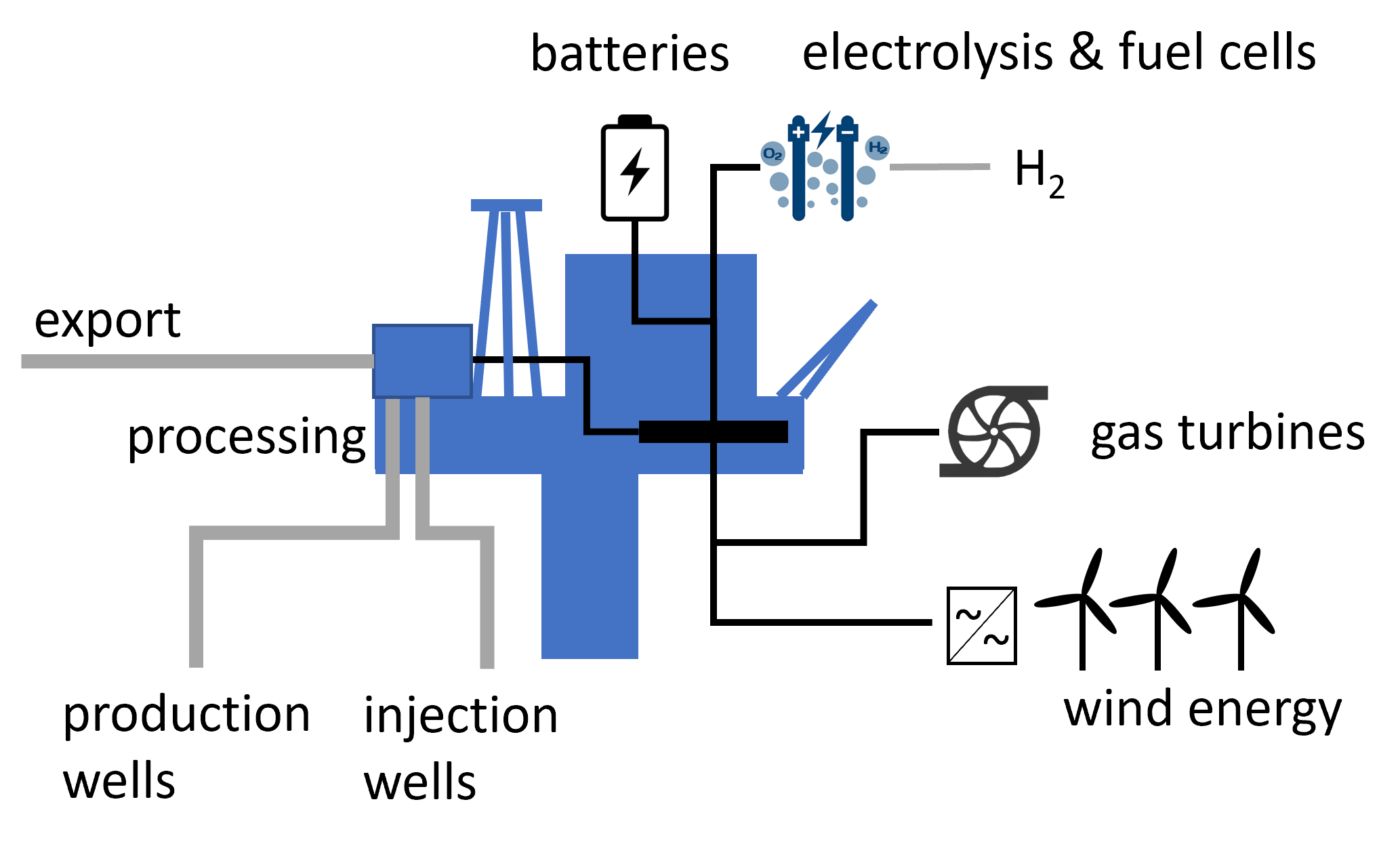
Figure 1: Offshore oil and gas platform with isolated energy system supplied partly by wind energy

2 An integrated model for energy system operation

For assessments of how different system designs and operating strategies influence offshore oil and gas platform energy system performance in terms of carbon emissions, fuel costs, oil and gas export rate etc, a new integrated energy system model has been developed and applied in simulation studies. This energy system model considers multiple energy and fluid flow carriers in offshore energy systems that may consist of multiple platforms connected together with pipelines and electric power cables. The integrated modelling is essential to capture the links between heat and power demand and oil and gas production and processing. These are important when studying how for example allowing load flexibility in combination with variable wind power supply can reduce emissions whilst maintaining production rates within specified limits. Details about this model are presented in the following.

2.1 Model overview

The purpose of the model is to allow fast and relatively simple analysis of the energy system, and to provide a convenient way to explore “what if” type questions. At its core, the model is an operational optimisation model that aims to identify optimal use of available flexible resources. Some examples of questions the model can address are: How are emissions affected if we add a wind turbine? How does it affect the number of gas turbine startups and shutdowns? What if we allow some flexibility in water injection pumps, how does that influence the need for energy storage? The emphasis is on the energy supply and distribution system. As mentioned above, energy consumption and its dependence on oil and gas transport and processing is also included, but typically represented on an aggregated level.

The model is a multi-energy optimisation model, partly inspired by the concept of energy hubs [28, 29]. The approach is familiar from previous studies of integrated energy systems, see e.g. [30, 31]. In most cases, such models are used for investment planning, whereas the application here is operational planning and comparisons of different system configurations and power management strategies in the operational phase.

2.2 Devices and networks

The basic building blocks in the model are devices and networks. Devices are all the individual components, such as gas turbine generators, compressors, pumps, auxiliary loads, separator trains, batteries, electrolysers, and others. Generally, devices connect a set of input and output flows of energy/matter. For example, a gas turbine takes gas input and gives electricity and heat output. Mathematical expressions relate these input/output flow quantities: Different sets of equations (and inequalities) describe the properties of the individual device types and the relationships between the input and the output. For computational efficiency, only linear relationships are considered in the model. All device types included in the model, with their respective input/output flows are illustrated in Figure 2. The mathematical expressions describing each device type are given in A.1.

Figure 2: Device types with their in/out flows

Devices are located at nodes that in turn are connected by edges (pipelines or cables) into networks. For each node, there is a set of inlet and outlet terminals, one for each network type. And devices and edges are connected via these terminals. Edges are distinguished by which type of flow they carry.

Edges of the same type make up a network of that type. That is, there is one network for each carrier, i.e. electricity, heat, oil, gas, water, hydrogen. The physical energy or matter flow through the networks may be described by different methods. The simplest is a transport model, where no constraints except upper and lower limits on each edge are included. More detailed linear flow models are also possible: For electricity, the linearised power flow equations relating power flow and nodal voltage could be used, and for fluids, the linearised Weymouth (for gas) or Darcy-Weissbach (for liquids) equations relating flow rates and pressure levels may be used.

Electrical losses may be accounted for via a piece-wise linear loss function relating power flow to power loss. This may have a significant impact in case of long distance electric power connections.

2.3 Optimisation problem

The equations and inequalities for all devices and networks are combined with an objective function into a mixed-integer linear programming (MILP) optimisation problem. Various elements may be included in the objective function, such as e.g. fuel consumption, carbon emission, and other operating costs. In general, the objective is to minimise a penalty, whose exact interpretation is determined by the user input.

The device and network equations or inequalities mentioned in Section 2.2 are constraints in the optimisation. The optimisation problem is solved sequentially, with energy storage, load flexibility and start-up delay linking different time-steps. The problem is solved by looping over time-steps, and updated between each step. Time-series profiles describe the variability where relevant, e.g. power availability for wind turbines, wellstream flow, power demand variations etc.

Schematically, the optimisation problem is defined as follows:

$$\begin{split}\min\sum_{d\in\mathbb{D}}\Bigl{[}&\sum_{t\in\mathbb{T}}\Bigl{\{}P^{d}(f_{d,c}^{i}(t),y^{d}_{\text{on}},y^{d}_{\text{prep}})+c^{d}_{\text{start}}y^{d}_{\text{start}}(t)+c^{d}_{\text{stop}}y^{d}_{\text{stop}}(t)\Bigr{\}}\\ &+c^{d}_{\text{storage}}\delta_{E}^{d}\Bigr{]}\\ \text{such that:}\\ &\text{all constraints are satisfied}\end{split}$$ (1)

where $\mathbb{D}$ is the set of devices, $\mathbb{T}$ is the set of time-steps in the optimisation horizon (see below), $f_{d,c}^{i}$ is the flow of carrier $c$ in or out ($i\in\{\text{in,out}\}$) of device $d$, $y^{d}_{\text{on}},y^{d}_{\text{prep}},y^{d}_{\text{start}},y^{d}_{\text{stop}}$ are binary variables indicating device on/off status (see below), $P^{d}(\dots)$ is a piece-wise linear penalty function for device $d$, $c^{d}_{\text{start}}$ is start-up penalty, $c^{d}_{\text{stop}}$ is shut-down penalty, $c^{d}_{\text{storage}}$ is storage depletion penalty, $\delta_{E}^{d}$ is the energy storage filling compared to a target value at the end of the optimisation horizon. The target value could be some value based on long-term storage utilisation planning. The penalty function $P^{d}$ may include fuel costs, CO₂ taxes or other costs (or negative incomes) as a function of input/output flows. A penalty for storage depletion is relevant when the model includes energy storage devices whose capacity is large compared to the optimisation horizon. Without such a penalty, the optimisation will not see a benefit of charging or filling the storage.

The constraints are spelled out in detail in A. In brief, they include relationships describing the devices, energy or matter balance in each terminal, network flow equations, and reserve power requirements.

2.4 Start-stop logic and rolling horizon

Optimised start and stop of gas turbine generators, and possibly other devices, can have a significant impact on the energy system performance. Since there is some preparation time from start-up decision to actual power output and potential limitations on ramping rates, forecasts and planning ahead is important. To keep track of on/off and activation status, four binary variables are used [32]. The decision variables are $y_{\text{start}}$ and $y_{\text{stop}}$, which are 1 if a decision to start or stop is made. The two derived variables $y_{\text{prep}}$ and $y_{\text{on}}$ indicate whether the device is in startup preparation or online respectively. This is illustrated in Figure 3 for an example with preparation time of 4 time-steps: The device is in preparation if it was started in the last 4 time-steps, and online if it was started 4 steps previously or online in the previous step and not stopped in the present step (see equation 4 and 5). A gas turbine generator consumes fuel also in the preparation phase, but provides electric power only when it is in the online state.

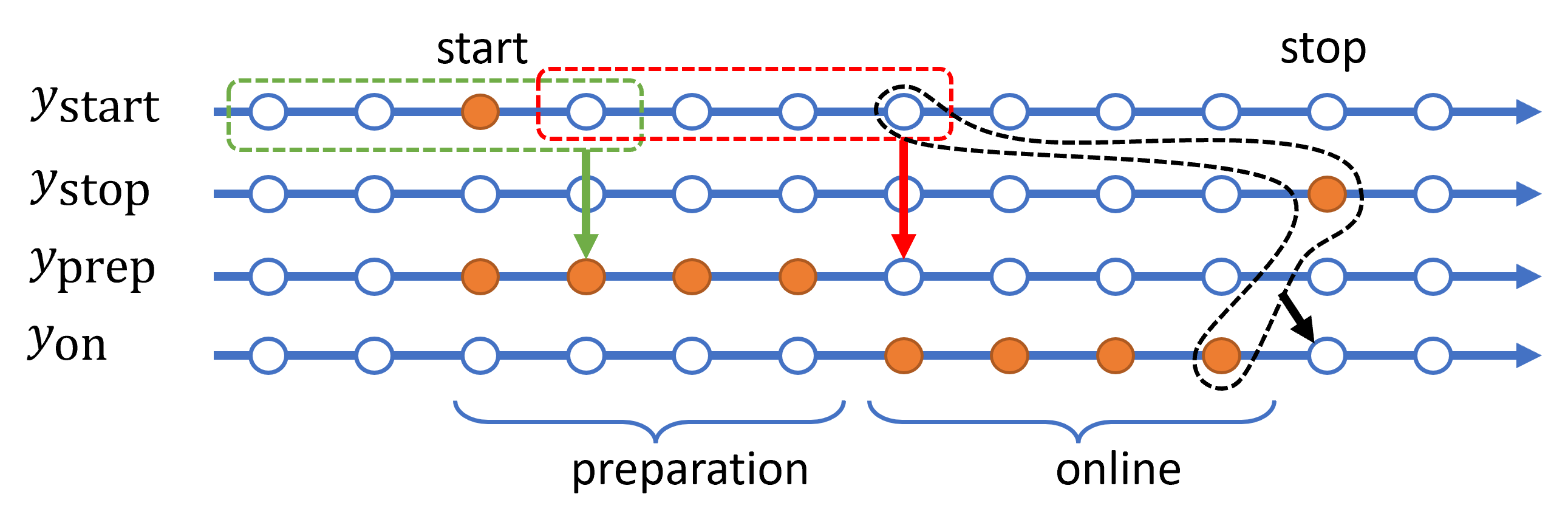
Figure 3: Start–stop logic. Illustrative example with a preparation time of 4 time-steps. Colouring of the dots indicate binary value 1 (orange) or 0 (white). The control variables $y_{\text{start}}$ and $y_{\text{stop}}$ determine the preparation and on/off status.

A rolling horizon optimisation is used to account for start-up delays, short-term flexibility in energy storage and energy demand, and the availability of improved forecasts closer to real-time. This means that the optimisation is repeated at regular intervals as time moves forward. This is illustrated in Figure 4. At a given time-step $t$, the system is optimised for a certain prediction horizon $(t,\dots,t+t_{H})$, where $t_{H}$ is the number of time-steps in the prediction horizon. Variable values for the first time step(s) represent decisions while values for later time steps are preliminary plans to be fixed or adjusted in subsequent iterations. In this figure, the optimisation is repeated every 2 time-steps, and the prediction horizon is 6 time-steps.

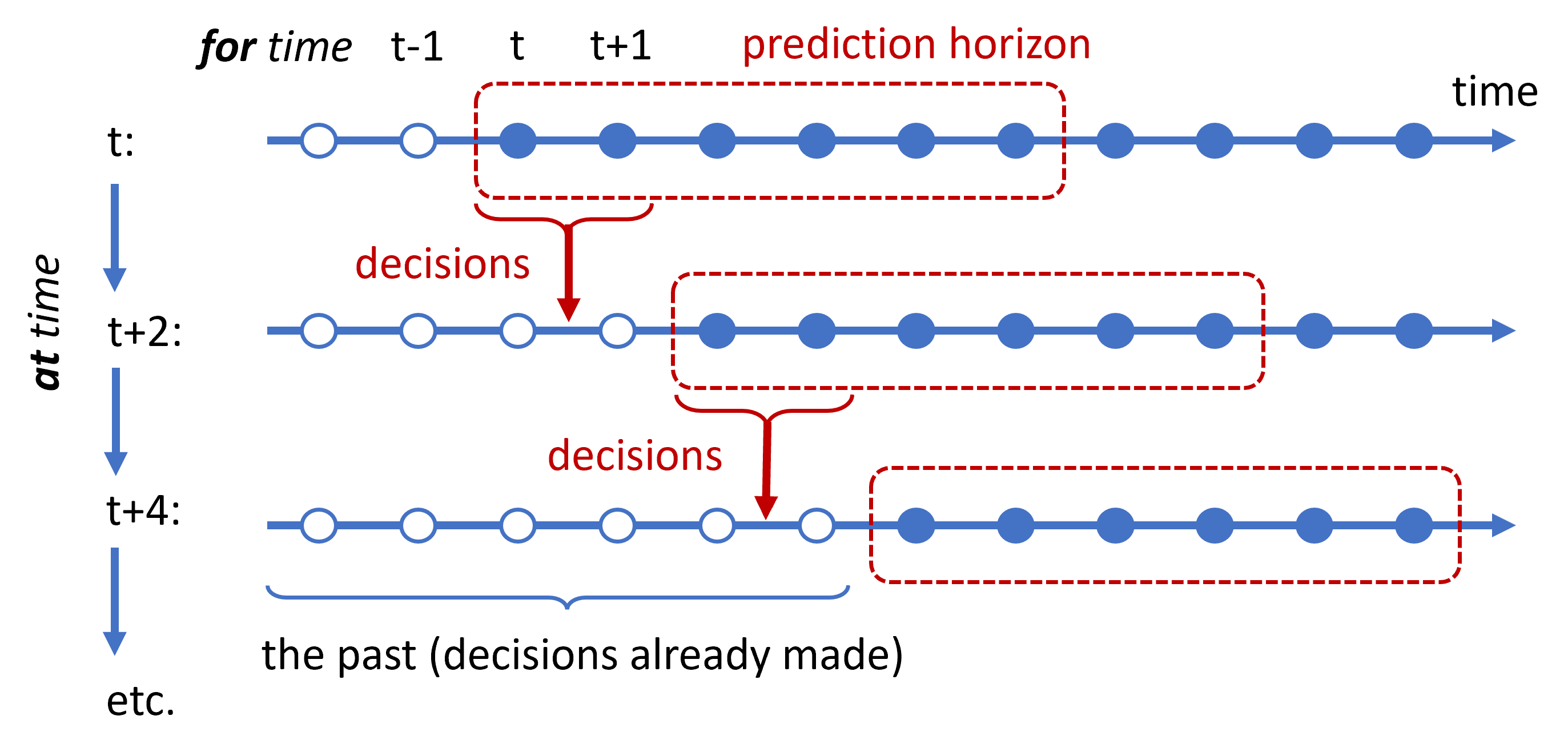
Figure 4: Rolling horizon optimisation with a prediction horizon of 6 time-steps, repeated every 2 time-steps (example)

2.5 The Oogeso tool

The above generic modelling concepts have been implemented as a new open source Python package named Offshore Oil and Gas Energy System Optimisation tool, or Oogeso for short [33].

This tool optimises system operation in the presence of variability and different sources of flexibility. Relevant decision variables are for example when to start-up or shut-down a gas turbine, when to charge or discharge a battery, or when to invoke load flexibility. In principle, it is an operational planning tool that identifies optimal set-points that can be fed into an energy management system. The main intended use, however, is to simulate offshore multi-energy systems and compute fuel consumption, greenhouse gas emissions, number of gas turbine starts and stops, and other key performance indicators, and use these to assess and compare simulation cases with different system designs or parameter choices reflecting different operating strategies. In this context, the purpose of the optimisation is to obtain a realistic operation of the system as part of a system analysis, rather than to identify optimal set-points in themselves.

It should be noted that the Oogeso tool is an energy system analysis tool, with only a simple representation of the oil and gas processing system, and that it does not include a reservoir model. However, it includes the connection between flow rates and energy demand for pumps and compressors which are crucial to address the potential for energy demand flexibility. The Oogeso tool allows devices and networks to be arranged in any way, making it suitable to analyse a broad range of different configurations without too much effort on the modelling side.

2.6 Online power reserve

An important system parameter affecting energy system operation is the required online power reserve (spinning reserve). This is power capacity reserved to balance unforeseen variations in demand and supply due to for example a motor start-up or wind forecast error. In traditional offshore power systems, only gas turbine generators provide reserve. In general, however, unused generator capacity, potential storage discharge capacity and potential load reduction may all contribute to the reserve. The reserve in an offshore energy system is typically not sufficient to cover all demand in case of a generator failure or other similar rare events. In those cases, frequency-based load shedding will be activated. The Oogeso model considers operational planning close to real-time, but not such real-time control actions.

3 Simulation setup

This section presents results from simulations of a relevant offshore oil and gas platform using the Oogeso tool described in the previous chapter.

The aim of the study is to assess and compare different alternatives for carbon emission reductions by adding wind energy supply to an existing platform, with and without energy storage. Additionally, this study demonstrates the applicability of the Oogeso analysis tool on a relevant case.

3.1 The LEOGO reference platform

The Low Emission Oil and Gas Open (LEOGO) reference platform [34] has been used as a basis for demonstrating the model and to analyse some alternatives for reducing carbon emissions. The LEOGO platform is a hypothetical but realistic case that is representative of a Norwegian offshore oil and gas production platform. It is well suited for our present purpose since the specification and associated data is public.

In brief, the LEOGO platform represents an oil and gas platform with production rates of $8600\text{\,}\mathrm{S}\mathrm{m}^{3}\mathrm{/}\mathrm{d}\mathrm{a}\mathrm{y}$ oil, $4.3\text{\,}\mathrm{m}\mathrm{i}\mathrm{l}\mathrm{l}\,~{}\mathrm{S}\mathrm{m}\mathrm{3}\mathrm{/}\mathrm{d}\mathrm{a}\mathrm{y}$ gas, and $13\,000\text{\,}\mathrm{S}\mathrm{m}\mathrm{3}\mathrm{/}\mathrm{d}\mathrm{a}\mathrm{y}$ water. The gas-to-oil ratio is 500 and the water cut is 0.6. Wellstream transport is supported by gas lift and reservoir pressure is maintained by water injection. Sea water is used in addition to production water for the water injection. Extracted oil and gas is exported via pipelines to a nearby platform. The main energy consumers are the gas compressors, oil export pumps, and water injection pumps. Electricity demand is about $40\text{\,}\mathrm{M}\mathrm{W}$, in the base case supplied by three gas turbines with active power rating of $21.8\text{\,}\mathrm{M}\mathrm{W}$. Heat demand is about $8\text{\,}\mathrm{M}\mathrm{W}$, supplied by gas turbine heat recovery.

The platform as represented in the Oogeso tool is illustrated in Figure 5.

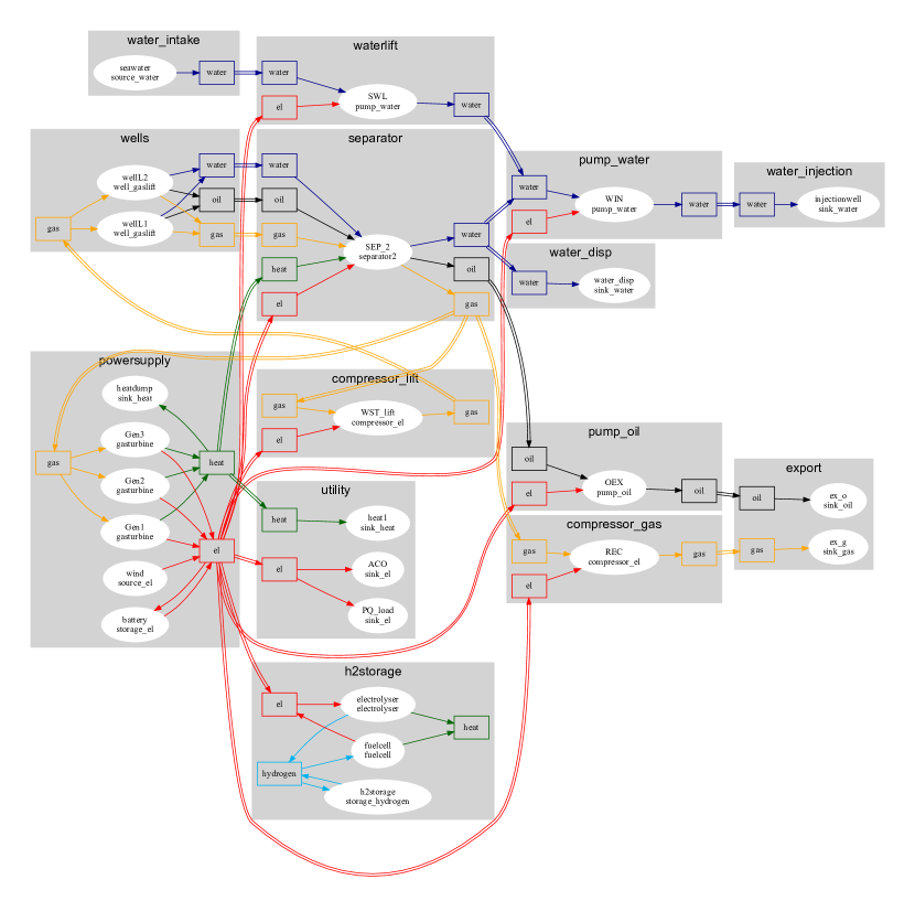
Figure 5: Overview of the LEOGO model implemented in Oogeso. Edge colours represent different energy carriers. Gray boxes are nodes and white ellipses are devices.

3.2 Energy demand and supply forecasts

In an energy management system with real-time operational optimisation, the best available forecasts for energy demand and supply would be used in each optimisation run. In a simulation setup, this is a bit different as the forecasts are given by input time-series up-front. To account for forecast errors when looking farther ahead, we use two different time-series for wind power: A forecast which represents the best prediction some time ahead, and a nowcast which represents the improved prediction for the next few minutes. In our case, the forecast has been generated from the nowcast simply by the addition of Gaussian noise.

In the simulations presented below, the nowcast was used for the first 10 minutes and the forecast was used for the rest of the optimisation horizon. This is a simplification of the real-world situation, but enables us to see the effect of forecast uncertainty to some extent.

Simulations were run for a one-week period, using wind speed data from the first week of April 2020, see Figure 6.

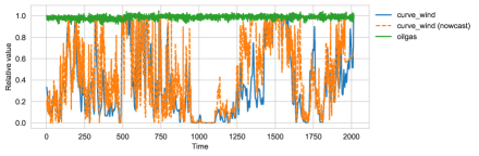
Figure 6: Time series profiles for wind forecasts and oil and gas production (wellstream flow rate)

3.3 Simulation cases

Four simulation cases, summarised in Table 3.3, have been defined. The base case corresponds to a typical present-day situation with power supply from local gas turbines. The three variations expand on this case with the addition of wind power, battery storage and hydrogen storage (via electrolyser and fuel cells). The battery storage is fairly small, but provides sufficient reserve power that a gas turbine may be allowed to switch off. The hydrogen storage is large enough to supply the full power demand for about 4 days. These simulation cases are chosen to illustrate some generic performance differences, but not selected in detail.

Table 1: Simulation cases

Base case	Variation A	Variation B	Variation C
3 gas turbines	3 gas turbines
24 MW wind power

& 3 gas turbines 24 MW wind power 4 MW/4 MWh battery 3 gas turbines 96 MW wind power Hydrogen storage

Table 2: Main simulation parameters

Parameter	Value
Time resolution	5 min
Time between each optimisation	30 min
Planning horizon	120 min
Reserve required	5 MW
Gas turbine generator max power	21.8 MW
Gas turbine generator min power	3.5 MW
Gas turbine generator startup time	30 min

For the simulations, time-steps of 5 minutes were used. This resolution is high enough to account for wind power variability and gas turbine generator start-up delays. Further key input parameters are given in Table 2. The full data and simulation settings are provided with the LEOGO dataset [34].

4 Results

An overview and comparison of simulation results is provided in Figure 7. The main observations from the simulations are elaborated in the following.

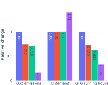
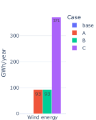
Figure 7: Simulation results

4.1 Emissions

CO₂ emission rates for the different simulation cases are compared to the base case in the first plot in Figure 7, and absolute numbers and time-variation are shown in Figure 8. In the base case, a more or less constant power demand is supplied by three gas turbine generators, and the emission rate is steady at close to $8\text{\,}\mathrm{k}\mathrm{g}\mathrm{C}\mathrm{O}_{\mathrm{2}}\mathrm{/}\mathrm{s}$. Wind power reduces gas turbine fuel usage and therefore emissions. The reduction is $25\text{\,}\%$ in variation A and $28\text{\,}\%$ in variation B. The slightly better performance in variation B is because the reserve provided by the battery makes it possible to switch off an extra gas turbine, thus allowing gas power generation at higher efficiency.

In Variation C, the wind power capacity has been increased to 96 MW with a total wind energy production similar to the energy demand. The electricity demand is increased by $41\text{\,}\%$ because of the electrolyser which produces hydrogen when there is excess wind power. Since there is no other heat source, one gas turbine is still needed to supply the heat demand and giving rise to CO₂ emissions. If waste heat recovery from the electrolyser and fuel cell or an electric heater were included instead, this would not be needed and the emission rate could be reduced to almost zero. The jump in emissions at time-step around 1200 is because of sustained low wind conditions where the hydrogen storage has run empty, see Figure 9. Therefore more power and even a second gas turbine is required for a short time.

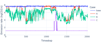
Figure 8: CO₂ emission rates

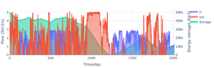
Figure 9: Hydrogen storage utilisation (Variation C). Flow in and out (left hand axis) and storage filling level (right-hand axis)

4.2 Gas turbine utilisation

Gas turbine running hours are compared in the third plot in Figure 7, and usage goes down as wind energy share increases. In this case, it is interesting to note that variation B with a battery has a significant improvement compared to variation A. The same is seen when comparing the number of starts (and stops) in the fourth plot. The reason for this is the $4\text{\,}\mathrm{M}\mathrm{W}$ online power reserve provided by the battery, which lowers the needed reserve from the gas turbines from $5\text{\,}\mathrm{M}\mathrm{W}$ to $1\text{\,}\mathrm{M}\mathrm{W}$ (sum). The gas turbines can therefore be run closer to maximum power, allowing one or two gas turbines to be shut-down more often in case B than in A. Both the gas turbine running hours and the number of starts and stops is therefore considerably less in variation B than in variation A. As noted above, in variation C, a single gas turbine is needed for the heat demand with minimal need for starts and stops.

It is clear from this that the relationship between the power demand, the gas turbine power capacity and the reserve requirement has a significant impact on emission reduction and number of gas turbine starts and stops. To obtain the maximum benefits, selecting the right capacities in the design phase and tuning of operational strategies is therefore important.

Figure 10 shows a time-series of power supply and start/stop status of the gas turbine generators in Variation A simulations. The gas turbines balance the variable wind power to cover the electricity demand which is just over 40 MW. The third gas turbine generator is only needed when wind power is low. Note that the power sharing between the online generators is not realistically represented in this plot, and is an artefact of the linear modelling: In reality, generator controls would ensure equal loading of the online generators.

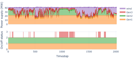
Figure 10: Power supply and generator start/stop status (Variation A)

4.3 Reserve

The impact of the battery on the reserve requirement is illustrated in more detail in Figure 11 which shows power supply and available reserve from each of the power sources in Variation A and Variation B. The importance of the reserve requirement is clear. The dotted red line shows the required margin of 5 MW, and the total online power reserve must be above this limit. Around time-step 950, the wind drops to zero, but even though the two gas generators has a combined capacity of 43.6 MW, a third power source is needed to provide sufficient power reserve. In Variation A this is done by starting up a third generator, whereas in Variation B, stored energy and power capacity of the battery provides the required reserve. In fact, in these simulations with fairly constant demand around 41 MW, we can easily deduce that the battery or a third generator is needed when the wind power forecast is less than about 2.4 MW.

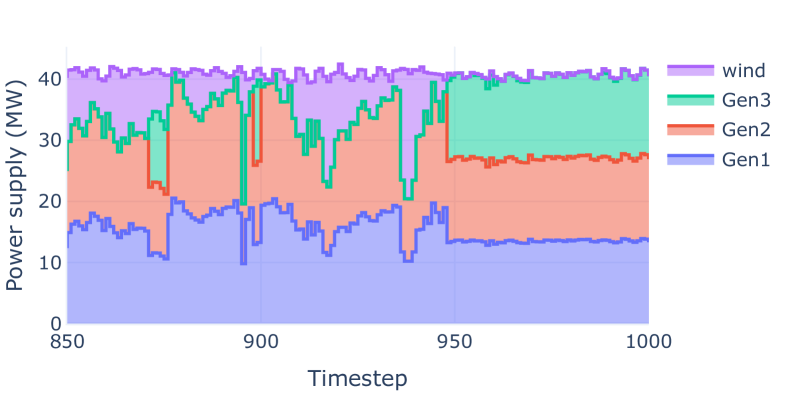
(a) Variation A – power supply

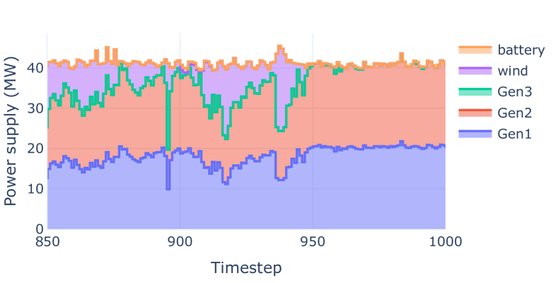
(b) Variation B – power supply

(c) Variation A – reserve

(d) Variation B – reserve

Figure 11: Comparison of power output (top) and available resrve (bottom) in Variations A and B. The battery in Variation B contributes to reserve and avoids the need for starting up an exta gas turbine at timestep 950.

5 Conclusion

The Oogeso open-source optimisation and simulation tool for analysis of energy system operation has been presented and demonstrated for a relevant offshore oil and gas platform case. It has proven useful to assess the effects of modifications in system configurations and operating parameters, such as e.g. wind power capacity, reserve requirement, energy storage capacity, and their impact on CO₂ emissions and other performance indicators.

The results have quantified the benefits of adding wind turbines and energy storage to reduce CO₂ emissions whilst satisfying electricity and heat demand within specified reserve safety margins. The case variations have been selected to illustrate key capabilities of the modelling approach and do not represent optimised alternatives. The details of the simulation results should be considered in light of this.

The work presented in this paper opens multiple directions for follow-on work. On the modelling side, planned future work will consider demand-side flexibility and how this can be efficiently represented in the operational optimisation model. Utilising load flexibility will be important to minimise the need for costly energy storage alternatives. Load flexibility may also lower the power reserve requirement. Another improvement would be to use forecast uncertainty and an option to determine the reserve requirement dynamically: If the forecast is uncertain, more reserve is needed. Although the Oogeso tool has been made for analyses of offshore oil and gas installations, the model is generic and can be used also for other types of multi-energy systems. To better represent thermal systems, the fluid temperature should be explicitly included, as well as thermal losses.

Acknowledgements

The work reported here has received financial support by the Research Council of Norway through PETROSENTER LowEmission (project code 296207) and through the OFFLEX project (project code 319158). Insightful comments on the manuscript by colleague Til K Vrana are greatly appreciated.

Appendix A Oogeso Optimisation problem constraints

The following sections describe in detail the equations and inequalities governing the energy system as represented in the Oogeso model, i.e. all the constraints in the optimisation problem that was outlined in Section 2.3. The constraints are grouped into constraints associated with devices, with networks (nodes or edges) and global constraints.

For questions regarding the exact implementation that are not clear from this presentation, the reader is pointed to the open-source code [33].

A.1 Device constraints

Devices are governed by some relationships that are generic and common for all device types, and some that are specific to each device type. The generic constraints, corresponding to max/min flow (e.g. power output) (2), ramp rate limits (3), and on/off status (4 and 5), are:

$$y_{\text{on}}f^{\text{min}}pr(t) \leq f\leq y_{\text{on}}f^{\text{max}}pr(t)$$ (2)

$$-r_{-}^{\text{max}} \leq\frac{f(t)-f(t-1)}{f^{\text{max}}\Delta t}\leq r_{+}^{\text{max}}$$ (3)

$$y_{\text{on}}(t)-y_{\text{on}}(t-1) =y_{\text{start}}(t-t_{s})-y_{\text{stop}}(t)$$ (4)

$$y_{\text{prep}}(t) =\sum_{\tau=0}^{t_{s}-1}y_{\text{start}}(t-\tau)$$ (5)

where $t$ is the time-step, $f$ is a flow variable whose definition depends on the device type (specified below), $f^{\text{max}}$ and $f^{\text{min}}$ are maximum and minimum flow limits, $pr(t)$ is a time-series profile (or 1 if no profile is specified $y_{\text{on}}$ and $y_{\text{prep}}$ are binary variables indicating whether the device is on or in preparatory (startup) phase, $y_{\text{start}}$ and $y_{\text{stop}}$ are bindary variables indicating wheter the device is starting or stopping, $t_{s}$ is the number of timestep the device spends in preparatory phase, $\Delta t$ is the timestep length, and $r_{\pm}^{\text{max}}$ is maximum up and downwards ramping limit.

The constraints specific to each type are given in the following.

Well

The well is the source for the combined oil/gas/water wellstream from the reservoir. The model allows for gas injection, whose purpose is to assist the wellstream flow. The set of governing equations are:

$$f =(f^{\text{out}}_{\text{gas}}-f^{\text{in}}_{\text{gas}})+f^{\text{out}}_{\text{oil}}+f^{\text{out}}_{\text{water}}$$ (6)

$$p^{\text{gas}}_{\text{out}}=p^{\text{oil}}_{\text{out}}=p^{\text{water}}_{\text{out}} =\hat{p}_{\text{separator}}$$ (7)

$$f^{\text{out}}_{\text{water}} =\frac{r_{w}}{1+R_{s}(1-r_{w})}f$$ (8)

$$f^{\text{out}}_{\text{oil}} =\frac{1-r_{w}}{1+R_{s}(1-r_{w})}f$$ (9)

$$f^{\text{out}}_{\text{gas}}-f^{\text{in}}_{\text{gas}} =\frac{R_{s}(1-r_{w})}{1+R_{s}(1-r_{w})}f$$ (10)

$$f^{\text{in}}_{\text{gas}} =r_{\text{inj}}f^{\text{out}}_{\text{oil}}$$ (11)

$$p^{\text{in}}_{\text{gas}} =\hat{p}_{\text{inj}}$$ (12)

where $f$ is the wellstream flow from the reservoir into the well, $\hat{p}_{\text{separator}}$ is the separator inlet pressure and assumed fixed. $R_{s}$ is the gas over oil ratio (GOR), $r_{w}$ is the water cut (WC) ratio, $r_{\text{inj}}$ is the gas injection ratio, which is assumed fixed, and $\hat{p}_{\text{inj}}$ is the gas injection pressure, which is also assumed fixed.

Separator

The separator train is the device that splits the composite wellstream into its individual gas, water and oil components. The representation here is a simple model where the heat and electricity demand are assumed proportional to the flow. The following equations describe separator devices:

$$f^{\text{out}}_{\text{oil}} =f^{\text{in}}_{\text{oil}}$$ (13)

$$f^{\text{out}}_{\text{gas}} =f^{\text{in}}_{\text{gas}}$$ (14)

$$f^{\text{out}}_{\text{water}} =f^{\text{in}}_{\text{water}}$$ (15)

$$p^{\text{gas}}_{\text{out}} =\hat{p}^{\text{gas}}_{\text{sep,out}}$$ (16)

$$p^{\text{oil}}_{\text{out}} =\hat{p}^{\text{oil}}_{\text{sep,out}}$$ (17)

$$p^{\text{water}}_{\text{out}} =\hat{p}^{\text{water}}_{\text{sep,out}}$$ (18)

$$f^{\text{in}}_{\text{heat}} =r_{\text{heat}}(f^{\text{in}}_{\text{oil}}+f^{\text{in}}_{\text{gas}}+f^{\text{in}}_{\text{water}})$$ (19)

$$f^{\text{in}}_{\text{el}} =r_{\text{el}}(f^{\text{in}}_{\text{oil}}+f^{\text{in}}_{\text{gas}}+f^{\text{in}}_{\text{water}})$$ (20)

where $r_{\text{heat}}$ is the heat demand factor, $r_{\text{el}}$ is the electricity demand factor, $\hat{p}^{\text{gas}}_{\text{sep,out}}$, $\hat{p}^{\text{oil}}_{\text{sep,out}}$, $\hat{p}^{\text{water}}_{\text{sep,out}}$ are nominal (assumed fixed) separator outlet pressures,

Compressor

Compressors are used to increase the pressure of natural gas, needed for gas lift and gas transport (export). The equation expressing the compressor power consumption is derived from the work done compressing the gas in an adiabatic process, assuming the ideal gas law. That gives the non-linear equation

$$\begin{split}P_{\text{compr}}(q,p_{\text{gas}}^{\text{in}},p_{\text{gas}}^{\text{out}})&=c\Bigl{[}(\frac{p_{\text{gas}}^{\text{out}}}{p_{\text{gas}}^{\text{in}}})^{a}-1\Bigr{]}q\\ &\quad a=\frac{k-1}{k}\\ &\quad c=\frac{\rho}{\eta_{is}}\frac{1}{k-1}ZRT_{1}\end{split}$$ (21)

where $q$ is the gas flow rate, $p_{1}$, $p_{2}$ is inlet/outlet pressure, $R$ is the individual gas constant, $\rho$ is gas density at standard conditions, $\eta_{is}$ is the isentropic efficiency of the compressor, $k$ is the specific heat capacity ratio, $Z$ is gas compressibility, and $T_{1}$ is inlet temperature.

The linearised version of this power demand function is:

$$P^{\text{linear}}_{\text{compr}}(q,p_{\text{gas}}^{\text{in}},p_{\text{gas}}^{\text{out}})=c\Bigl{[}a(\frac{\hat{p}^{\text{out}}}{\hat{p}^{\text{in}}})^{a}\hat{q}(\frac{p^{\text{out}}}{\hat{p}^{\text{out}}}-\frac{p^{\text{in}}}{\hat{p}^{\text{in}}})+((\frac{\hat{p}^{\text{out}}}{\hat{p}^{\text{in}}})^{a}-1)q\Bigr{]}$$ (22)

For an electric compressor we therefore get the following constraints

$$f^{\text{gas}}_{\text{out}} =f^{\text{gas}}_{\text{in}}$$ (23)

$$f^{\text{in}}_{\text{el}} =P^{\text{linear}}_{\text{compr}}(f_{\text{gas}}^{\text{out}},p_{\text{gas}}^{\text{in}},p_{\text{gas}}^{\text{out}})$$ (24)

and for a gas-driven compressor:

$$f^{\text{gas}}_{\text{out}} =f^{\text{gas}}_{\text{in}}-\frac{1}{c_{\text{gas}}}P^{\text{linear}}_{\text{compr}}(f_{\text{gas}}^{\text{out}},p_{\text{gas}}^{\text{in}},p_{\text{gas}}^{\text{out}})$$ (25)

where $c_{\text{gas}}$is the gas calorific value (combustible energy content).

Pumps

Power consumption by oil or water pumps can be computed considering the work needed to move the liquid up a pressure gradient. For an incompressible liquid, the result is

$$P_{\text{pump}}(q)=\frac{1}{\eta_{\text{pump}}}(p^{\text{out}}-p^{\text{in}})q\approx\frac{1}{\eta_{\text{pump}}}(\hat{p}^{\text{out}}-\hat{p}^{\text{in}})q$$ (26)

where $q$ is the flow rate, $\eta_{\text{pump}}$ is the pump efficiency, and we have assumed that pressure levels are close to nominal values $\hat{p}$ This gives the pump equations:

$$f^{\text{out}} =f^{\text{in}}$$ (27)

$$f^{\text{in}}_{\text{el}} =P_{\text{pump}}(f^{\text{in}})$$ (28)

Gas turbine generators

Gas turbine generators use gas to generate electricity and heat. The equations expressing their relaionships are:

$$f =f_{\text{el}}^{\text{out}}$$ (29)

$$\frac{f_{\text{gas}}^{\text{in}}}{f^{\text{max}}}c_{\text{gas}} =A\frac{f_{\text{el}}^{\text{out}}}{f^{\text{max}}}+B(y_{\text{on}}+y_{\text{prep}})$$ (30)

$$f_{\text{heat}}^{\text{out}} =(f_{\text{gas}}^{\text{in}}c_{\text{gas}}-f_{\text{el}}^{\text{out}})\eta_{\text{heat}}$$ (31)

where $f_{\text{gas}}^{\text{in}}$, $f_{\text{el}}^{\text{out}}$ and $f_{\text{heat}}^{\text{out}}$ are variables describing the flow in/out of the device, $c_{\text{gas}}$ is the gas energy content (MJ/Sm3), $A$ and $B$ are dimensionless coefficients that specify the linear fuel consumption curve.

Heater

For electric heaters (boilers or heat pumps), the equation relating electricity consumption and heat output is

$$f =f_{\text{el}}^{\text{in}}$$ (32)

$$f_{\text{heat}}^{\text{out}} =\eta f_{\text{el}}^{\text{in}}$$ (33)

where $\eta$ is the el-to-heat efficiency.

Sources

These device only have an equation defining the flow variable $f$ used in the generic device constraints, depending on source type:

$$f=f^{\text{in}}_{\text{c}},\quad c\in\{\text{oil},\text{gas},\text{water},\text{el},\text{heat},\text{hydrogen}\}$$ (34)

Sinks

As for sources, sink device only have an equation defining the flow variable $f$ used in the generic device constraints, depending on which sink type:

$$f=f^{\text{in}}_{\text{c}},\quad c\in\{\text{oil},\text{gas},\text{water},\text{el},\text{heat},\text{hydrogen}\}$$ (35)

Battery storage

The constraints for battery storage are:

$$f =f_{\text{el}}^{\text{out}}$$ (36)

$$(\eta f_{\text{el}}^{\text{in}}-\frac{1}{\eta}f_{\text{el}}^{\text{out}})\Delta t =E(t)-E(t-1)$$ (37)

$$E^{\text{min}}\leq E\leq E^{\text{max}}$$ (38)

$$f^{\text{out}}_{\text{el}} \leq f^{\text{max}}$$ (39)

$$f^{\text{in}}_{\text{el}} \leq-f^{\text{min}}$$ (40)

$$p^{\text{max}} =\min\{f^{\text{max}},\frac{E}{t_{\text{res}}}\}$$ (41)

where $\Delta t$ is the timestep duration, $\eta$ is the charge/discharge efficiency, $E(t)$ is the storage energy content at timestep $t$, and $t_{\text{res}}$ is the minimum time the power must be available to count towards reserve. The variable $p^{\text{max}}$ gives the maximum available power from the the storage, a quantity needed to compute the power reserve. It is limited both by the discharge capacity and by the energy in the storage.

The equation with the minimum value function is represented by the linear equations

$$f^{\text{max}}-M(1-y_{\text{storage}}) \leq p^{\text{max}}\leq f^{\text{max}}$$ (42)

$$\frac{E}{t_{\text{res}}}-My_{\text{storage}} \leq p^{\text{max}}\leq\frac{E}{t_{\text{res}}}$$ (43)

where $y_{\text{storage}}$ is a binary helper variable, $M$ is a large (big-M) parameter (larger than $f^{\text{max}}$). The binary variable $y$ will be 1 if $\frac{E}{t_{\text{res}}}<f^{\text{max}}$, and 0 otherwise.

Hydrogen storage

The hydrogen storage model is somewhat simpler than battery storage because the charging/discharging is represented by separate units (electrolyser and fuel cell). Its equations are

$$f =f_{\text{hydrogen}}^{\text{out}}$$ (44)

$$(f_{\text{hydrogen}}^{\text{in}}-f_{\text{el}}^{\text{out}})\Delta t =E(t)-E(t-1)$$ (45)

$$E^{\text{min}} \leq E\leq E^{\text{max}}$$ (46)

$$\delta_{E} \geq-(E-E_{\text{target}})$$ (47)

where $\delta_{E}$ is a non-negative variable representing the energy storage deviation from the target value $E_{\text{target}}$ at the end of the optimisation horizon.

The storage deviation constraints are associated with the storage depletion penalty in the objective function (Eq. 1).

Electrolyser

These devices produce hydrogen and heat from electricity:

$$f =f^{\text{el}}_{\text{in}}$$ (48)

$$f^{\text{hydrogen}}_{\text{out}}c_{h} =f^{\text{el}}_{\text{in}}\eta_{\text{h}}$$ (49)

$$f^{\text{heat}}_{\text{out}} =f^{\text{el}}_{\text{in}}(1-\eta_{\text{h}})\eta_{\text{heat}}$$ (50)

where $c_{h}$ is the hydrogen calorific value (energy content), $\eta_{\text{h}}$ is the electrolyser efficiency, and $\eta_{\text{heat}}$ is the waste heat recovery efficiency.

Fuelcells

These produce electricity and heat from hydrogen:

$$f =f^{\text{el}}_{\text{out}}$$ (51)

$$f^{\text{el}}_{\text{out}} =f^{\text{hydrogen}}_{\text{in}}c_{h}\eta_{\text{cell}}$$ (52)

$$f^{\text{heat}}_{\text{out}} =f^{\text{hydrogen}}_{\text{in}}c_{h}(1-\eta_{\text{cell}})\eta_{\text{heat}}$$ (53)

where $c_{h}$ is the hydrogen calorific value (energy content), $\eta_{\text{cell}}$ is the fuel cell efficiency, and $\eta_{\text{heat}}$ is the waste heat recovery efficiency.

A.2 Network constraints

The following sections give the network-related constraints.

A.2.1 Flow balance at each node terminal

Edges to the node $n$ are always connected to the in terminal and edges from the node are always connected to the out terminal. Therefore, for each node $n$ and carrier $c$ the total flow into the ”in” terminal and out of the ”out” terminal are given as the contributions from the connected devices and edges as:

in: $$F^{\text{in}}_{c}=-\sum_{d\in\mathbb{D}_{n}}f_{\text{d,c}}^{\text{in}}+\sum_{e\in\mathbb{E}^{\text{to}}_{c,n}}(q_{e}-q_{e,+}^{\text{loss}})-q^{\text{term}}_{c,n}=0$$ (54)

out: $$F^{\text{out}}_{c}=-\sum_{d\in\mathbb{D}_{n}}f_{\text{d,c}}^{\text{out}}+\sum_{e\in\mathbb{E}^{\text{from}}_{c,n}}(q_{e}+q_{e,-}^{\text{loss}})-q^{\text{term}}_{c,n}=0$$ (55)

where $\mathbb{D}_{n}$ is the set of devices at node $n$, $\mathbb{E}_{c,n}^{\text{from}}$ is the set of edges of carrier $c$ going from node $n$, $\mathbb{E}_{c,n}^{\text{to}}$ is the set of edges of carrier $c$ going to node $n$.

The term $q^{\text{term}}_{c,n}$ is only present if there are no devices connecting both the in and the out terminal for a given carrier $c$ (and therefore have device constraints specifying the flow between them). It is used and is used to effectively merge the in/out terminals to a single terminal.

A.2.2 Electrical losses

To account for (electrical) losses, the edge flow, which in general can be positive or negative, is split in two always non-negative variables $q_{+}$and $q_{-}$, such that

$$q =q_{+}-q_{-}$$ (56)

Only one of these components will be non-zero at any time.

We define the flow components such that $q_{+}$ is the flow in positive direction out of the “from” end and $q_{-}$ is the flow in negative direction out of the “to” end. Losses are calculated via a piece-wise linear function $F^{\text{loss}}$:

$$q_{+}^{\text{loss}}=F^{\text{loss}}(q_{+}),\qquad q_{-}^{\text{loss}}=F^{\text{loss}}(q_{-}),\qquad q^{\text{loss}}=q_{+}^{\text{loss}}+q_{-}^{\text{loss}}.$$ (57)

The general expressions for edge flow out of the “from” end ($q^{\text{from}}$) and into the “to” end ($q^{\text{to}}$) are:

$$q^{\text{from}} =q_{+}-(q_{-}-q_{-}^{\text{loss}})=q+q_{-}^{\text{loss}}$$ (58)

$$q^{\text{to}} =(q_{+}-q_{+}^{\text{loss}})-q_{-}=q-q_{+}^{\text{loss}}$$ (59)

A.2.3 Fluid pressure deviation limit

Limits on the deviation of pressure from the nominal value (given through input data) may be added for fluid flows. For example, if the gas pressure at the export point, or the water injection pump output pressure should have a fixed value, this may be enforced in this way. The associated constraint is given as:

$$p_{n,c}^{\text{nom}}(1-\delta_{n,c}^{\text{max}}) \leq p_{n,c}\leq p_{n,c}^{\text{nom}}(1+\delta_{n,c}^{\text{max}})$$ (60)

where $p_{n,c}$ is the pressure for carrier $c$ at node $n$, $p_{n,c}^{\text{nom}}$ is nominal pressure, and $\delta_{n,c}^{\text{max}}$ is the maximum allowable relative pressure deviation from the nominal value (0–1).

A.2.4 Edge flow limits

Edges may be specified as bidirectional, which is generally the case for electric flow, or one-directional, which is generally the case for fluids:

$$-q^{\text{max}} \leq q\leq q^{\text{max}}\qquad(\text{bidirectional})$$ (61)

$$0 \leq q\leq q^{\text{max}}\qquad(\text{one-directional})$$ (62)

where $q$ is the edge flow, $q^{\text{max}}$ is the maximum flow (in either direction).

A.2.5 Edge flow equations

The simplest way to represent edge flow is as a transport model, where the flow is constrained only by upper and lower bounds, and by energy/matter balance in the endpoint nodes.

However, for extended networks with a meshed electricity grid or long-distance pipelines, it may be necessary to use more advanced models relating voltage angles and power flow for electric networks, or flow rate and pressure for pipeline fluid flows are possible. These are described below.

Electric power flow

Power flow in an electricity grid is determined by the locations of power injection and ejection and the impedances of the alternative routes. The equations describing this are the non-linear AC power flow equations. A linearised version of these equations gives a good approximation if voltages are close to nominal values, phase angle differences are small and resistances are small compared to reactances. The linearised equations, in matrix form and expressed using dimensionless per unit quantities, are

$$\mathbf{Q}=\mathbf{DA\Theta},$$ (63)

where $\mathbf{Q}=[q_{1},\dots,q_{m}]$ is a vector of edge power flow, $\mathbf{D}=\text{diag}(-\frac{1}{x_{1}},\dots,-\frac{1}{x_{m}})$ is a diagonal matrix with elements given by the edge reactances, $A$ is the $m\times n$-dimensional node–branch incidence matrix describing the network topology, $\mathbf{\Theta}=[\theta_{1},\dots,\theta_{n}]$ is the vector of nodal voltage angles, and $m$ is the number of edges and $n$ is the number of nodes.

In addition to the above equation, it is necessary to define a reference node $n_{\text{ref}}$ for voltage angles such that $\theta_{n_{\text{ref}}}=0$.

Gas flow

The empirical Weymouth equation is appropriate for describing pressure drop in gas pipelines with large diameter, at high pressure, and high flow rates [35], and is used if pressure drop in gas pipelines is considered in the model. The equation relates flow rate and pressure in and out:

$$q=k\sqrt{\left(p_{1}^{2}-e^{s}p_{2}^{2}\right)},$$ (64)

where $q$ is the edge fluid flow rate, $p_{1}$ and $p_{2}$ are inlet and outlet pressure, $\exp(s)$ is a constant factor that accounts for elevation differences (see below), and $k$ is a pipeline property constant given as:

$$k=4.3328\cdot 10^{-8}\frac{\mathrm{m}^{\mathrm{3}}}{\mathrm{\text{s MPa}}}\cdot\frac{T_{b}}{P_{b}}\left[GT_{f}L_{e}Z\right]^{-\frac{1}{2}}D^{\frac{8}{3}},$$ (65)

where $D$ is pipe diameter (in mm), $T_{b}$ is base temperature (ambient temperature) (in K), $P_{b}$ is base pressure (local atmosphere) (in MPa), $G$ is the gas gravity constant, $T_{f}$ is the gas temperature, and $Z$ is the compressibility factor.

The factor $e^{s}$ and the equivalent length $L_{e}$ together account for elevation differences. These are defined as:

$$s=0.0684G\frac{z_{2}-z_{1}}{T_{f}Z},$$ (66)

$$L_{e}=L\frac{e^{s}-1}{s},$$ (67)

where $z$ is elevation (in m) and $L$ is the segment length (km).

It is assumed here that the pressure remains close to the given nominal values $\hat{p}_{1}$ and $\hat{p}_{2}$ at the pipe endpoints. The non-linear Weymouth equation is then linearised around these points, [36]

$$p_{1}=\hat{p}_{1}+\Delta p_{1},\quad p_{2}=\hat{p}_{2}+\Delta p_{2},$$ (68)

giving the linear equation:

$$q=\frac{k}{\sqrt{\left(\hat{p}_{1}^{2}-e^{s}\hat{p}_{2}^{2}\right)}}\left[\hat{p}_{1}p_{1}-e^{s}\hat{p}_{2}p_{2}\right],$$ (69)

that relates flow rate $q$ and pressure at start $p_{1}$ and endpoint $p_{2}$.

Liquid flow

The pressure loss in an incompressible fluid (liquid) pipeline due to friction is described by the empirical Darcy-Weisbach equation [35]:

$$p_{2}-p_{1}=-\rho g(z_{2}-z_{1})-f_{D}\frac{\rho L}{D}\frac{V^{2}}{2},$$ (70)

where $p_{1}$ and $p_{2}$ are inlet and outlet pressure, $V$ is average fluid velocity, $z$ is elevation, $\rho$ is fluid density, $g=9.98~{}\text{m}/\text{s}^{2}$ is the gravity constant, $L$ is the pipe length, $D$ is the pipe diameter, and $f_{D}$ is the Darcy friction factor.

Since the velocity $V$ is related to the volumetric flow rate $q$, this can be written as

$$p_{2}-p_{1}=-\rho g(z_{2}-z_{1})-\frac{8f_{D}\rho Lq^{2}}{\pi^{2}D^{5}}.$$ (71)

The Darcy friction factor $f_{D}$ is determined by pipe properties and flow regime. It can be computed in different ways, but in our model is assumed given as user input.

Linearising this equation around an operating point given by the nominal pressure values $\hat{p}_{1},\hat{p}_{2}$ and flow rate $\hat{q}$ (derived from the equation above), we get a linear equation that relates flow rate and in/out pressure for liquid pipeline flow:

$$p_{2}-p_{1}= -(q-\hat{q})\frac{2X}{k}+(\hat{p}_{2}-\hat{p}_{1})$$ (72)

$$X=\sqrt{(\hat{p}_{1}-\hat{p}_{2})-\rho g(z_{2}-z_{1})}$$ (73)

$$k=\sqrt{\frac{\pi^{2}D^{5}}{8f_{D}\rho L}}$$ (74)

$$\hat{q}=kX$$ (75)

Note that for this linear approximation to be good, the flow rate needs to be close to the nominal value. If conditions change, the coefficients should be updated.

A.3 Global constraints

In addition to constraints associated with devices and the networks, the optimisation problem may includes global constraints as explained in the following.

Reserve margin limit

Power reserve is the online available power capacity that is not used. Both generators and loads may contribute reserve. The reserve requirement constraint is:

$$\sum_{d\in\mathbb{D}}(f_{\text{d,el}}^{\text{max}}x_{d}^{\text{res}}-f_{\text{d,el}}^{\text{out}}+f_{\text{d,el}}^{\text{in}}x_{d}^{\text{L,res}})\geq R^{\text{L,min}}$$ (76)

where $\mathbb{D}$ is the set of devices, $f_{\text{d,el}}^{\text{max}}$ is the maximum available electric power output for device d, $x_{d}^{\text{res}}$ is a reserve factor parameter (0–1) that determines how much of the unused capacity should count towards the reserve, $x_{d}^{\text{L,res}}$ is a parameter (0–1) that determines how much of the load can be reduced, $R^{\text{min}}$ is the minimum reserve limit (MW).

For a generator, the reserve factor is typically 1, but may be less if for example there is uncertainty in the estimation of available capacity, as is the case for wind power. For loads, the reserve factor $x_{d}^{\text{L,res}}$ is 0 if no load shedding is allowed.

Emission rate limit

The CO₂ emission rate is the emission per time. If a hard limit on emissions should be enforced, an emission rate limit may be specified through the equation:

$$\sum_{d\in\mathbb{D}_{gas}}c_{\text{CO${}_{2}$ }}(f_{\text{d,gas}}^{\text{in}}-f_{\text{d,gas}}^{\text{out}})\leq e_{\text{CO${}_{2}$ }}^{\text{max}}$$ (77)

where $\mathbb{D}_{gt}$ is the set of gas-combusting devices (gas turbine generators and gas-driven compressors), $c_{\text{CO${}_{2}$ }}$ is gas CO₂ content (kg/Sm3), and $e_{\text{CO${}_{2}$ }}^{\text{max}}$ is the CO₂ emission rate limit (kg/s).

References

-
[1]
H. Devold,
Oil
and gas production handbook. An introduction to oil and gas production,
transport, refining and petrochemical industry, ABB Oil and Gas, 2013.
URL https://search.abb.com/library/Download.aspx?DocumentID=9AKK104295D4314&LanguageCode=en&DocumentPartId=&Action=Launch - [2] T.-V. Nguyen, M. Voldsund, P. Breuhaus, B. Elmegaard, Energy efficiency measures for offshore oil and gas platforms, Energy 117 (2016) 325–340, the 28th International Conference on Efficiency, Cost, Optimization, Simulation and Environmental Impact of Energy Systems - ECOS 2015. doi:https://doi.org/10.1016/j.energy.2016.03.061.
- [3] M. Voldsund, T.-V. Nguyen, B. Elmegaard, I. S. Ertesvåg, A. Røsjorde, K. Jøssang, S. Kjelstrup, Exergy destruction and losses on four north sea offshore platforms: A comparative study of the oil and gas processing plants, Energy 74 (2014) 45–58. doi:https://doi.org/10.1016/j.energy.2014.02.080.
- [4] S. Roussanaly, A. Aasen, R. Anantharaman, B. Danielsen, J. Jakobsen, L. Heme-De-Lacotte, G. Neji, A. Sødal, P. Wahl, T. Vrana, R. Dreux, Offshore power generation with carbon capture and storage to decarbonise mainland electricity and offshore oil and gas installations: A techno-economic analysis, Applied Energy 233-234 (2019) 478–494. doi:https://doi.org/10.1016/j.apenergy.2018.10.020.
- [5] L. O. Nord, R. Anantharaman, A. Chikukwa, T. Mejdell, Ccs on offshore oil and gas installation - design of post-combustion capture system and steam cycle, Energy Procedia 114 (2017) 6650–6659, 13th International Conference on Greenhouse Gas Control Technologies, GHGT-13, 14-18 November 2016, Lausanne, Switzerland. doi:https://doi.org/10.1016/j.egypro.2017.03.1819.
- [6] L. Riboldi, S. Völler, M. Korpås, L. O. Nord, An integrated assessment of the environmental and economic impact of offshore oil platform electrification, Energies 12 (11) (2019). doi:10.3390/en12112114.
- [7] E. Æsøy, J. G. Aguilar, S. Wiseman, M. R. Bothien, N. A. Worth, J. R. Dawson, Scaling and prediction of transfer functions in lean premixed h2/ch4-flames, Combustion and Flame 215 (2020) 269–282. doi:https://doi.org/10.1016/j.combustflame.2020.01.045.
- [8] Gas Turbines or Electric Drives in Offshore Applications, Vol. Volume 4: Turbo Expo 2005 of Turbo Expo: Power for Land, Sea, and Air. doi:10.1115/GT2005-68003.
- [9] T. Mäkitie, H. E. Normann, T. M. Thune, J. Sraml Gonzalez, The green flings: Norwegian oil and gas industry’s engagement in offshore wind power, Energy Policy 127 (2019) 269–279. doi:https://doi.org/10.1016/j.enpol.2018.12.015.
- [10] Equinor, Hywind tampen, https://www.equinor.com/en/what-we-do/hywind-tampen.html, accessed 2021-07-02 (2021).
- [11] M. Korpås, L. Warland, W. He, J. O. G. Tande, A case-study on offshore wind power supply to oil and gas rigs, Energy Procedia 24 (2012) 18–26. doi:https://doi.org/10.1016/j.egypro.2012.06.082.
- [12] W. He, G. Jacobsen, T. Anderson, F. Olsen, T. D. Hanson, M. Korpås, T. Toftevaag, J. Eek, K. Uhlen, E. Johansson, The potential of integrating wind power with offshore oil and gas platforms, Wind Engineering 34 (2) (2010) 125–137. doi:10.1260/0309-524X.34.2.125.
- [13] Q. Zhang, H. Zhang, Y. Yan, J. Yan, J. He, Z. Li, W. Shang, Y. Liang, Sustainable and clean oilfield development: How access to wind power can make offshore platforms more sustainable with production stability, Journal of Cleaner Production 294 (2021) 126225. doi:https://doi.org/10.1016/j.jclepro.2021.126225.
- [14] H. G. Svendsen, M. Hadiya, E. V. Øyslebø, K. Uhlen, Integration of offshore wind farm with multiple oil and gas platforms, in: 2011 IEEE Trondheim PowerTech, 2011, pp. 1–3. doi:10.1109/PTC.2011.6019309.
- [15] A. R. Årdal, T. Undeland, K. Sharifabadi, Voltage and frequency control in offshore wind turbines connected to isolated oil platform power systems, Energy Procedia 24 (2012) 229–236, selected papers from Deep Sea Offshore Wind R&D Conference, Trondheim, Norway, 19-20 January 2012. doi:https://doi.org/10.1016/j.egypro.2012.06.104.
- [16] D. Hu, X. Zhao, X. Cai, J. Wang, Impact of wind power on stability of offshore platform power systems, in: 2008 Third International Conference on Electric Utility Deregulation and Restructuring and Power Technologies, 2008, pp. 1688–1692. doi:10.1109/DRPT.2008.4523677.
- [17] J. I. Marvik, E. V. Øyslebø, M. Korpås, Electrification of offshore petroleum installations with offshore wind integration, Renewable Energy 50 (2013) 558–564. doi:https://doi.org/10.1016/j.renene.2012.07.010.
- [18] M. L. Kolstad, K. Sharifabadi, A. R. Årdal, T. M. Undeland, Grid integration of offshore wind power and multiple oil and gas platforms, in: 2013 MTS/IEEE OCEANS - Bergen, 2013, pp. 1–7. doi:10.1109/OCEANS-Bergen.2013.6608004.
- [19] X. Xie, J. Zhong, Y. Sun, J. Wang, C. Wei, Online optimal power control of an offshore oil-platform power system, Technology and Economics of Smart Grids and Sustainable Energy 3 (2018). doi:10.1007/s40866-018-0056-7.
- [20] E. F. Alves, D. d. S. Mota, E. Tedeschi, Sizing of hybrid energy storage systems for inertial and primary frequency control, Frontiers in Energy Research 9 (2021) 206. doi:10.3389/fenrg.2021.649200.
- [21] D. d. S. Mota, E. Tedeschi, On adaptive moving average algorithms for the application of the conservative power theory in systems with variable frequency, Energies 14 (4) (2021). doi:10.3390/en14041201.
- [22] D. d. S. Mota, E. Tedeschi, Understanding the effects of exponentially decaying dc currents on the dual dq control of power converters in systems with high x/r, in: 2021 IEEE 15th International Conference on Compatibility, Power Electronics and Power Engineering (CPE-POWERENG), 2021, pp. 1–6. doi:10.1109/CPE-POWERENG50821.2021.9501204.
- [23] S. Sanchez, E. Tedeschi, J. Silva, M. Jafar, A. Marichalar, Smart load management of water injection systems in offshore oil and gas platforms integrating wind power, IET Renewable Power Generation 11 (9) (2017) 1153–1162. doi:https://doi.org/10.1049/iet-rpg.2016.0989.
- [24] T.-V. Nguyen, B. Elmegaard, L. Pierobon, F. Haglind, P. Breuhaus, Modelling and analysis of offshore energy systems on north sea oil and gas platforms, in: Proceedings of the 53rd SIMS conference on Simulation and Modelling, 2012, sIMS 2012, 53rd Conference on Simulation and Modelling.
- [25] A. Zhang, H. Zhang, M. Qadrdan, W. Yang, X. Jin, J. Wu, Optimal planning of integrated energy systems for offshore oil extraction and processing platforms, Energies 12 (4) (2019). doi:10.3390/en12040756.
- [26] R. McKenna, M. D’Andrea, M. G. González, Analysing long-term opportunities for offshore energy system integration in the danish north sea, Advances in Applied Energy 4 (2021) 100067. doi:https://doi.org/10.1016/j.adapen.2021.100067.
- [27] H. Zhang, A. Tomasgard, B. R. Knudsen, H. G. Svendsen, S. J. Bakker, I. E. Grossmann, Modelling and analysis of offshore energy hubs, preprint: https://arxiv.org/abs/2110.05868 (2021). arXiv:2110.05868.
- [28] M. Geidl, G. Andersson, Optimal power flow of multiple energy carriers, IEEE Transactions on Power Systems 22 (1) (2007) 145–155. doi:10.1109/TPWRS.2006.888988.
- [29] A. Zhang, H. Zhang, M. Qadrdan, X. Li, Q. Li, Energy hub based electricity generation system design for an offshore platform considering co2-mitigation, Energy Procedia 142 (2017) 3597–3602, proceedings of the 9th International Conference on Applied Energy. doi:https://doi.org/10.1016/j.egypro.2017.12.250.
- [30] B. H. Bakken, H. I. Skjelbred, O. Wolfgang, etransport: Investment planning in energy supply systems with multiple energy carriers, Energy 32 (9) (2007) 1676–1689. doi:https://doi.org/10.1016/j.energy.2007.01.003.
- [31] I. van Beuzekom, M. Gibescu, J. Slootweg, A review of multi-energy system planning and optimization tools for sustainable urban development, in: 2015 IEEE Eindhoven PowerTech, 2015, pp. 1–7. doi:10.1109/PTC.2015.7232360.
- [32] E. Castillo, A. J. Gonejo, P. Pedregal, R. Garciá, N. Alguacil, Mixed-Integer Linear Programming, John Wiley & Sons, Ltd, 2001, Ch. 2, pp. 25–46. doi:https://doi.org/10.1002/9780471225294.ch2.
- [33] H. G. Svendsen, M. D. Aslesen, Offshore oil and gas energy system operational optimisation (oogeso) software code v1.0.0 (2022). doi:10.5281/zenodo.5971182.
- [34] H. G. Svendsen, A. Holdyk, T. K. Vrana, Leogo reference platform dataset v1.0 (2022). doi:10.5281/zenodo.5970656.
- [35] E. Menon, Gas Pipeline Hydraulics, CRC Press, 2005. doi:10.1201/9781420038224.
- [36] A. Tomasgard, F. Rømo, M. Fodstad, K. Midthun, Optimization models for the natural gas value chain, in: G. Hasle, K.-A. Lie, E. Quak (Eds.), Geometric Modelling, Numerical Simulation, and Optimization: Applied Mathematics at SINTEF, Springer Berlin Heidelberg, Berlin, Heidelberg, 2007, pp. 521–558. doi:10.1007/978-3-540-68783-2_16.