PCENet: High Dimensional Surrogate Modeling for Learning Uncertainty

Abstract

Learning data representations under uncertainty is an important task that emerges in numerous machine learning applications. However, uncertainty quantification (UQ) techniques are computationally intensive and become prohibitively expensive for high-dimensional data. In this paper, we present a novel surrogate model for representation learning and uncertainty quantification, which aims to deal with data of moderate to high dimensions. The proposed model combines a neural network approach for dimensionality reduction of the (potentially high-dimensional) data, with a surrogate model method for learning the data distribution. We first employ a variational autoencoder (VAE) to learn a low-dimensional representation of the data distribution. We then propose to harness polynomial chaos expansion (PCE) formulation to map this distribution to the output target. The coefficients of PCE are learned from the distribution representation of the training data using a maximum mean discrepancy (MMD) approach. Our model enables us to (a) learn a representation of the data, (b) estimate uncertainty in the high-dimensional data system, and (c) match high order moments of the output distribution; without any prior statistical assumptions on the data. Numerical experimental results are presented to illustrate the performance of the proposed method.

1 Introduction

Learning the input-output (I/O) relations of a given data system is a fundamental problem presents in several applications including supervised learning, solving and learning partial differential equations (PDEs), control systems, signal processing, computer vision, natural language processing, and many more. In recent times, Neural-Networks (NNs) have popularly been used for this purpose, and have been shown to be comprehensive and highly effective in these applications Goodfellow et al. (2016); Han et al. (2018); Deng and Liu (2018); Fadlullah et al. (2017); Voulodimos et al. (2018). In many situations, the tasks of learning data representation and I/O relationship also need to account for the uncertainty in the data (known as aleatoric/data uncertainty) and/or the system (known as epistemic/model uncertainty). Thus, the learning model should also offer means to perform uncertainty quantification (UQ) Smith (2013). For example, uncertainty in the data arises due to reasons such as noise, training and testing data mismatch, incomplete data, class overlap, discordant, multi-modal data and others Malinin (2019); Abdar et al. (2021). On the other hand, uncertainty in the model/system occurs due to inadequate knowledge, incorrect assumptions upon data distributions and/or model functions, natural variability in system parameters, faulty sub-systems and more Abdar et al. (2021); Schobi et al. (2015).

Given the importance of the problem, numerous methods for uncertainty modeling and quantification have been proposed in different engineering fields Smith (2013); Sullivan (2015) and the artificial intelligence literature Abdar et al. (2021). Traditional UQ techniques are typically stochastic sampling-based simulation methods Mohamed et al. (2010). However, these methods are computationally very expensive, making them inadequate for modern large and complex data models. Alternatively, surrogate modelling (also known as response surface or meta-model) techniques such as Polynomial Chaos Expansions (PCEs) Ghanem and Spanos (1990); Xiu and Karniadakis (2002); Soize and Ghanem (2004), Gaussian process modelling and regression Rasmussen (2003); Chen et al. (2015), and Support Vector Machines Li et al. (2006) have received much attention due to their low computational cost. Recently, deep learning methods Tripathy and Bilionis (2018); Zhang et al. (2019); Zheng et al. (2021), including Bayesian neural networks Wang and Yeung (2016); Abdar et al. (2021) have been used as surrogate models for UQ. However, parameterizing and training most of these surrogate models will be intractable when the number of input parameters is large (known as the "curse of dimensionality" Verleysen and Francois (2005)), i.e., for high-dimensional data systems.

Proposed approach:

In this paper, we design a surrogate modeling approach to learn representations of high-dimensional data systems under uncertainty. Our approach is to learn the functional mapping between the distributions of the input and output data, where both distributions could be unknown a-priori. This assists in data uncertainty modeling and propagation, as well as in promoting generalizability Wilson and Izmailov (2020). The proposed method comprises of two stages. In the first stage, we map the (possibly high-dimensional) input data distribution to a low-dimensional latent distribution using a NN approach. Then, in the second stage, a surrogate model is trained to learn a mapping between the latent and the output distributions. For the dimensionality reduction stage, we employ Variational Autoencoders (VAE) Kingma and Welling (2013), a NN-based Bayesian unsupervised learning approach. VAE embeds/maps the (possibly unknown) input data distribution to a normal distribution in a lower latent dimension, enabling us to use a suitable surrogate model to map the latent space to the output. VAE also helps in uncertainty propagation, and has recently been used for input data uncertainty quantification Böhm et al. (2019); Mehrasa et al. (2019); Guo et al. (2020).

In the surrogate modeling stage, we consider Polynomial Chaos Expansions (PCEs) Xiu and Karniadakis (2002); Ghanem and Spanos (1990); Oladyshkin and Nowak (2012) to learn the mapping from the latent distribution to the output space. PCEs are highly efficient uncertainty modeling techniques and have many appealing properties, including: (a) they are inexpensive to compute; (b) they can match higher-order moments, making them suitable for arbitrary distributions with arbitrary probability measures Oladyshkin and Nowak (2012); and (c) they capture the global characteristic of the function Schobi et al. (2015). We propose a maximum mean discrepancy (MMD) approach Gretton et al. (2012) to learn the coefficients of PCE from the training data. MMD is a moment matching technique, and therefore, enables us to match high order moments of the output distribution to the model response. Moreover, our approach only requires to sample the latent distribution, and does not require any prior statistical assumptions on the data.

In the learning set-up, we have a dataset $({\mathbf{x}}_{1},y_{1}),\ldots,({\mathbf{x}}_{n},y_{n})$ where $\{{\mathbf{x}}_{i}\}_{i=1}^{n}\in\mathcal{X}\subseteq\mathbb{R}^{m}$ and $\{y_{i}\}_{i=1}^{n}\in\mathcal{Y}\subseteq\mathbb{R}$, and a function $F:\mathcal{X}\longrightarrow\mathcal{Y}$, parameterized by ${\bm{\mathrm{\rho}}}$ (that may depend on the priors of $\{\mathcal{X},\mathcal{Y\}}$), such that the observations satisfy $y_{i}=F({\mathbf{x}}_{i},{\bm{\mathrm{\rho}}})$. We assume that $F$ is expensive to evaluate, and thus our goal is to build a cheap-to-compute function $\tilde{F}:\mathbb{R}^{m}\to\mathbb{R}$ that approximates $F$ well with respect to ${\bm{\mathrm{\rho}}}$, e.g., $|F-\tilde{F}|$ has a small ${\bm{\mathrm{\rho}}}$-weighted $\ell_{2}$ norm, which is expensive to evaluate. Our proposed model consists of two stages. In the first stage, we use a dimensionality reduction function $E:\mathbb{R}^{m}\to\mathbb{R}^{d}$ that maps $\{{\mathbf{x}}_{1},\dots,{\mathbf{x}}_{n}\}$ to $\{{\mathbf{z}}_{1},\dots,{\mathbf{z}}_{n}\}$ of a lower dimension with a new distribution ${\bm{\mathrm{\eta}}}$. Here, we set the latent dimension (a hyperparameter) $d$ to be much smaller than the input dimension $m$. The function $E$ will hence be the encoder part of VAE Kingma and Welling (2013). In the second stage, we construct a family of multivariate polynomials $\left\{\varphi_{j}\right\}_{j=1}^{N}$ which are orthogonal w.r.t. the distribution ${\bm{\mathrm{\eta}}}$, and the coefficients of the corresponding PCE are learned using the MMD approach (a kernel regression task) in order to map $\{{\mathbf{z}}_{1},\dots,{\mathbf{z}}_{n}\}$ to $\{y_{1},\dots,y_{n}\}$. The PCE function $P:\mathbb{R}^{d}\to\mathbb{R}$ has an expansion of the form

$$P({\bm{\mathrm{{\mathbf{z}}}}})=\sum_{j=1}^{N}c_{j}\varphi_{j}({\bm{\mathrm{{\mathbf{z}}}}}),$$

where $\varphi_{j}(\cdot)$’s are the orthogonal polynomials and $c_{j}$’s are coefficients learned using the MMD approach. Therefore, the proposed surrogate model can be written as $\tilde{F}({\mathbf{x}})=P\circ E({\mathbf{x}})=P({\bm{\mathrm{{\mathbf{z}}}}})$.

Outline:

In section 2, we provide details on notation as well as background information required for our method. We also discuss some of the prior works that are closely related to our approach. In section 3, we present the proposed method PCE-Net for learning data representation under uncertainty, and discuss the theoretical motivation and characteristics of the method. Numerical simulation results on a few datasets from different applications illustrating the performance of PCE-Net are presented in section 4.

2 Preliminaries

In this section, we first present the notation details and definitions. We then briefly discuss the three main ingredients of our proposed PCE-Net model, namely, Variational Autoencoder (VAE), Polynomial Chaos Expansion (PCE), and Maximum Mean Discrepancy (MMD). We end the section with a discussion on some of the related prior works.

2.1 Notation

We will follow the standard notation of lowercase, bold lowercase and bold uppercase letters for scalars $x$, vectors ${\mathbf{x}}$, and matrices ${\bm{\mathrm{X}}}$, respectively. Probability vector spaces are denoted using bold calligraphic letters $\mathcal{X}$ and functions using uppercase letters $F(\cdot)$. $D_{KL}$ denotes the Kullback-Leibler divergence (KL-divergence), and $f_{\bm{\mathrm{X}}}(\cdot)$ denotes the joint probability density function with ${\bm{\mathrm{X}}}$. Finally, $\mathcal{N}\left({\bm{\mathrm{\mu}}},{\bm{\mathrm{\Sigma}}}\right)$ denotes the multivariate Gaussian distribution with mean vector ${\bm{\mathrm{\mu}}}$ and covariance matrix ${\bm{\mathrm{\Sigma}}}$.z

2.2 Variational Autoencoder

VAE was first introduced by Kingma and Welling (2013), and is an unsupervised learning technique based on dimensionality reduction and variational inference (VI) Hinton and Van Camp (1993); Waterhouse et al. (1996); Jordan et al. (1998). VAE comprises of two parts. The first part is the encoder parameterized by ${\bm{\mathrm{\phi}}}$ which takes input ${\mathbf{x}}\in\mathbb{R}^{m}$ and returns a distribution on the latent variable ${\mathbf{z}}\in\mathbb{R}^{d}$, where $d<m$. The second part is the decoder parametrized by ${\bm{\mathrm{\theta}}}$ which tries to reconstruct ${\mathbf{x}}$ from the samples of the latent distribution. Together with VI, the encoder is the inference model and the decoder is the generative model. These two parts/NNs are jointly optimized in order to maximize the evidence lower bound (ELBO):

$$\begin{split}\cal{L}\left({\bm{\mathrm{\theta}}},{\bm{\mathrm{\phi}}};{\mathbf{x}}\right)&=\mathbb{E}_{q}\left[\ln p_{{\bm{\mathrm{\theta}}}}({\mathbf{x}},{\mathbf{z}})-\ln q_{{\bm{\mathrm{\phi}}}}({\mathbf{z}}|{\mathbf{x}})\right]\\ &=\ln p({\mathbf{x}})-D_{KL}\left[q_{{\bm{\mathrm{\phi}}}}({\mathbf{z}}|{\mathbf{x}})||p({\mathbf{z}}|{\mathbf{x}})\right]\\ &\leq\ln p({\mathbf{x}})\end{split}$$ (1)

where $\ln p({\mathbf{x}})$ is the marginal likelihood, and $D_{KL}$ is the KL-divergence.

In VI, an intractable posterior distribution $p_{{\bm{\mathrm{\theta}}}}({\mathbf{z}}|{\mathbf{x}})$ of a latent variable model $p_{{\bm{\mathrm{\theta}}}}({\mathbf{x}},{\mathbf{z}})=p_{{\bm{\mathrm{\theta}}}}({\mathbf{x}}|{\mathbf{z}})p({\mathbf{z}})$ is approximated by a guide $q_{{\bm{\mathrm{\phi}}}}({\mathbf{z}}|{\mathbf{x}})$. The approximation, $q_{{\bm{\mathrm{\phi}}}}({\mathbf{z}}|{\mathbf{x}})$, is performed by taking $q_{{\bm{\mathrm{\phi}}}}({\mathbf{z}}|{\mathbf{x}})$ to be a simple distribution, e.g., Gaussian with a diagonal covariance $\cal{N}\left({\bm{\mathrm{\mu}}}({\mathbf{x}}),{\bm{\mathrm{\Sigma}}}({\mathbf{x}})\right)$. The parameters of $q_{{\bm{\mathrm{\phi}}}}({\mathbf{z}}|{\mathbf{x}})$ are estimated by maximizing Eq. (1). In VAE, the encoder outputs $q_{{\bm{\mathrm{\phi}}}}({\mathbf{z}}|{\mathbf{x}})$ by returning ${\bm{\mathrm{\mu}}}({\mathbf{x}})$ and (the diagonal elements of) ${\bm{\mathrm{\Sigma}}}({\mathbf{x}})$, and then ${\mathbf{z}}$ is sampled and passed through the decoder which allows the optimization of the ELBO.

Importantly, ELBO can also be written as

$$\mathcal{L}\left({\bm{\mathrm{\theta}}},{\bm{\mathrm{\phi}}};{\mathbf{x}}\right)=\mathbb{E}_{q}\left[\ln p_{{\bm{\mathrm{\theta}}}}({\mathbf{x}}|{\mathbf{z}})\right]-D_{KL}\left[q_{{\bm{\mathrm{\phi}}}}({\mathbf{z}}|{\mathbf{x}})||p({\mathbf{z}})\right]$$ (2)

where $p({\mathbf{z}})$ is some predetermined prior distribution. The term $D_{KL}\left[q_{{\bm{\mathrm{\phi}}}}({\mathbf{z}}|{\mathbf{x}})||p_{{\bm{\mathrm{\theta}}}}({\mathbf{z}})\right]$ can be viewed as a regularization term which forces $q_{{\bm{\mathrm{\phi}}}}({\mathbf{z}}|{\mathbf{x}})$ to be approximately distributed as the prior $p({\mathbf{z}})$, which is independent of ${\mathbf{x}}$. Thus, $q_{{\bm{\mathrm{\phi}}}}({\mathbf{z}})$ is approximately distributed as the prior. Typically, the prior is chosen to be $p({\mathbf{z}})=\cal{N}\left(\mathbf{0},{\bm{\mathrm{I}}}\right)$.

2.3 Polynomial Chaos Expansion

Polynomial Chaos Expansion (PCE) is an inexpensive surrogate model that aims to map uncertainty from an input space $\mathcal{X}\subseteq\mathbb{R}^{m}$ to an output space $\mathcal{Y}\subseteq\mathbb{R}$. The uncertainty is expressed through a probabilistic framework using random vectors, i.e., ${\bm{\mathrm{Y}}}=P({\bm{\mathrm{X}}})$ where ${\bm{\mathrm{X}}}\in\cal{X}$ with a given joint probability density function (PDF) $f_{\bm{\mathrm{X}}}(\cdot)$ and $P(\cdot)$ is a sum of polynomials that are typically orthogonal w.r.t. the measure $f_{\bm{\mathrm{X}}}$ Ghanem and Spanos (1990); Xiu and Karniadakis (2002); Soize and Ghanem (2004). In contrast to other probabilistic methods such as Gaussian processes, PCEs approximate the global behavior of the model using a set of orthogonal polynomials. It is also assumed that ${\bm{\mathrm{Y}}}$ has a finite variance $\mathbb{E}[{\bm{\mathrm{Y}}}^{2}]<\infty$, and that each component of ${\bm{\mathrm{X}}}$ has finite moments of any order.

Thus, the space of square integrable functions w.r.t. the weighted function $f_{\bm{\mathrm{X}}}(\cdot)$ can be represented by an orthonormal basis of polynomials $\{\varphi_{{\bm{\mathrm{i}}}}(\cdot)\}_{{\bm{\mathrm{i}}}\in\mathbb{N}^{m}}$:

$$\int_{\cal{X}}\varphi_{{\bm{\mathrm{i}}}}({\mathbf{x}})\varphi_{{\bm{\mathrm{j}}}}({\mathbf{x}})f_{\bm{\mathrm{X}}}({\mathbf{x}})=\delta_{{\bm{\mathrm{ij}}}}\,.$$ (3)

Therefore, ${\bm{\mathrm{Y}}}$ can be represented as

$${\bm{\mathrm{Y}}}=P({\bm{\mathrm{X}}})=\sum_{{\bm{\mathrm{j}}}\in\mathbb{N}^{m}}c_{{\bm{\mathrm{j}}}}\varphi_{{\bm{\mathrm{j}}}}({\bm{\mathrm{X}}})\,.$$ (4)

The coefficients $c_{{\bm{\mathrm{j}}}}$ in (4) are usually computed using a data driven regression approach Schobi et al. (2015); Torre et al. (2019); Lataniotis et al. (2020). Given a dataset of observations $({\mathbf{x}}_{1},y_{1}),\dots,({\mathbf{x}}_{n},y_{n})\in\mathcal{X}\times\mathcal{Y}$, the coefficients can be found by regression fitting, such as by minimizing the $L_{2}$ loss function

$$\sum_{i=1}^{n}\left(y_{i}-P({\mathbf{x}}_{i})\right)^{2}.$$

Crucially, the orthonormality of the basis implies that the squared sum of the PCE coefficients typically displays rapid decay, which in turn reduces the number of coefficients actually required and thus avoids overfitting.

Furthermore, in the case where the components of ${\bm{\mathrm{X}}}$ are independent and identically distributed, the polynomials in (4) are composed of univariate polynomials by tensor product:

$$\varphi_{{\bm{\mathrm{j}}}}({\bm{\mathrm{X}}})=\prod_{k=1}^{m}\varphi_{j_{k}}^{(k)}(X_{k})$$ (5)

where $\varphi_{j_{k}}^{(k)}$ is the $j_{k}$ polynomial in the $k$-th dimension. Since using the series (4) is not practical, PCE is used as a surrogate that replaces the true model in practice. This is done by truncating the series such that $|{\bm{\mathrm{j}}}|=\sum_{k=1}^{N}j_{k}\leq N$:

$$P_{N}({\bm{\mathrm{X}}})=\sum_{j=1}^{N_{p}}c_{j}\varphi_{j}({\bm{\mathrm{X}}})$$ (6)

where the number of coefficients is

$$N_{p}=\frac{(N+m)!}{N!m!}\,.$$

It can be seen that for a large dimension $m$, the process becomes prohibitively expensive.

2.4 Maximum Mean Discrepancy

Gretton et al. (2012) presented a metric for measuring distances between distributions in terms of mean embedding, which they termed maximum mean discrepancy (MMD) . Let $\cal{H}$ be a reproducing kernel Hilbert space (RKHS) over the domain $\cal{X}$ and $K:\cal{X}\times\cal{X}\to\mathbb{R}$ be the associated kernel. Denote ${\bm{\mathrm{\mu}}}_{{\bm{\mathrm{\eta}}}}=\mathbb{E}_{x\sim{\bm{\mathrm{\eta}}}}[K({\mathbf{x}},\cdot)]$ as the kernel mean of a given probability measure ${\bm{\mathrm{\eta}}}$ over $\cal{X}$. Then, for two probability measures ${\bm{\mathrm{\eta}}}$ and ${\bm{\mathrm{\nu}}}$ over $\cal{X}$, with mean embeddings ${\bm{\mathrm{\mu}}}_{{\bm{\mathrm{\eta}}}}$ and ${\bm{\mathrm{\mu}}}_{{\bm{\mathrm{\nu}}}}$ respectively, the MMD is:

$$\text{MMD}({\bm{\mathrm{\eta}}},{\bm{\mathrm{\nu}}})=\|{\bm{\mathrm{\mu}}}_{{\bm{\mathrm{\eta}}}}-{\bm{\mathrm{\mu}}}_{{\bm{\mathrm{\nu}}}}\|_{{\cal H}}^{2}\,$$

and can also be expressed as

$$\text{MMD}({\bm{\mathrm{\eta}}},{\bm{\mathrm{\nu}}})=\mathbb{E}_{{\bm{\mathrm{\eta}}}}\left[K({\mathbf{x}},{\mathbf{x}}^{\prime})\right]-2\mathbb{E}_{{\bm{\mathrm{\eta}}},{\bm{\mathrm{\nu}}}}\left[K({\mathbf{x}},{\mathbf{y}})\right]+\mathbb{E}_{{\bm{\mathrm{\nu}}}}\left[K({\mathbf{y}},{\mathbf{y}}^{\prime})\right]\,.$$

where ${\mathbf{x}},{\mathbf{x}}^{\prime}\sim{\bm{\mathrm{\eta}}}$ and ${\mathbf{y}},{\mathbf{y}}^{\prime}\sim{\bm{\mathrm{\nu}}}$. It can be seen that MMD is zero only if the two distributions are equal.

Given two sets of samples ${\bm{\mathrm{X}}}=\{{\mathbf{x}}_{i}\}_{i=1}^{n_{1}}$ and ${\bm{\mathrm{Y}}}=\{{\mathbf{y}}_{i}\}_{i=1}^{n_{2}}$, one may ask whether their distributions ${\bm{\mathrm{\eta}}}$ and ${\bm{\mathrm{\nu}}}$ are the same. For that purpose, an empirical estimate of MMD can be obtained by

$${\cal L}_{{MMD}^{2}}=\frac{1}{n_{1}^{2}}\sum_{i,j=1}^{{n_{1}}}K({\mathbf{x}}_{i},{\mathbf{x}}_{j})-\frac{2}{{n_{1}}{n_{2}}}\sum_{i=1}^{n_{1}}\sum_{j=1}^{n_{2}}K({\mathbf{x}}_{i},{\mathbf{y}}_{j})+\frac{1}{n_{2}^{2}}\sum_{i,j=1}^{n_{2}}K({\mathbf{y}}_{i},{\mathbf{y}}_{j})\,.$$ (7)

Note that, as a consequent, the resulting kernel mean may incorporate high order moments of ${\bm{\mathrm{\eta}}}$. For example, when the kernel $K(\cdot,\cdot)$ is linear, $\mathbb{E}_{{\bm{\mathrm{\eta}}}}[K]={\bm{\mathrm{\mu}}}_{{\bm{\mathrm{\eta}}}}$ is simply the mean of ${\bm{\mathrm{\eta}}}$. Thus, choosing a Gaussian kernel allows us to capture high-order moments, and MMD acts as a moment matching approach, see Li et al. (2015); Kiasari et al. (2017) for details.

2.5 Related Work

In this section we discuss some of the prior works in the literature that are closely related to our proposed approach. PCEs as surrogate models (SM) have been popularly used for data driven uncertainty quantification and sensitivity analysis in numerous applications Xiu and Karniadakis (2002); Crestaux et al. (2009); Najm (2009); Sepahvand et al. (2010); Duong et al. (2016); Torre et al. (2019); Ubaru et al. (2021). Arbitrary PCE Oladyshkin and Nowak (2012) has been proposed to handle data with arbitrary and unknown distributions, and sparse PCE Blatman and Sudret (2011) was proposed for reducing the computational cost of PCEs. Schobi et al. (2015) proposed a method named PC-Krigging that combines PCEs with Gaussian processes for improved global-local representation of the given data system. However, as previously mentioned, such surrogate modeling approaches are not applicable for high-dimensional data systems.

The idea of using dimensionality reduction (DR) methods for uncertainty quantification of high-dimensional data systems has been considered in the UQ literature Ghanem and Spanos (2003), and DR methods such as principal component analysis (PCA), kernel PCA Ma and Zabaras (2011), active subspace methods Constantine et al. (2015) and autoencoders Mehrasa et al. (2019) have been used. Tripathy et al. (2016) proposed an active subspace approach (DR method) that is combined with a Gaussian process (SM method) for high-dimensional uncertainty propagation. Later, Lataniotis et al. (2020) presented a general framework for Dimensionality Reduction Surrogate Modelling (DRSM) approach for UQ, and studied various combinations of DR (PCA and kernel PCA) and SM (PCE and Gaussian processes) methods for UQ. Their approach is to approximate the input data using a kernel density estimation, and then use a relative generalization error for learning the SM. Deep neural network based surrogate models have been proposed by Tripathy and Bilionis (2018); Zheng et al. (2021) for high dimensional uncertainty quantification. However, our approach differs from these methods in multiple aspects, namely: (a) our approach is to learn the mapping between input and output distributions, and not that of the given training input and output data (better generalization); (b) we directly learn the distributions of the data in the latent space and do not use kernel density estimation (significant computational cost gain); and (c) we use a moment matching approach to learn the coefficients of the SM (improved output distribution matching).

3 PCE-Net

In this section, we present the proposed method PCE-Net for high-dimensional uncertainty quantification. The method follows the DRSM approach and (a) uses VAE for learning a distribution of the input data in a low-dimensional latent space, (b) then considers a PCE surrogate model to map the latent space to the output, and (c) uses MMD to learn the coefficients of PCE.

We begin by training a VAE on the given input data $\{{\mathbf{x}}_{1},\dots,{\mathbf{x}}_{n}\}$. The learned parameters ${\bm{\mathrm{\phi}}}$ of the encoder allow each of the data points ${\mathbf{x}}_{i},\,i=1,\dots,n$ to generate a distribution $\mathcal{N}\left({\bm{\mathrm{\mu}}}_{i},{\bm{\mathrm{\Sigma}}}_{i}\right)$, from which the corresponding ${\mathbf{z}}_{1},\dots,{\mathbf{z}}_{n}\in\mathbb{R}^{d}$ can be sampled. We denote by $E_{{\bm{\mathrm{\phi}}}}(\cdot)$ the encoder and sampling operations which map each data point ${\mathbf{x}}_{i}$ to a low dimensional sample ${\mathbf{z}}_{i}$.

In the next stage, we consider the $d$ components of ${\mathbf{z}}_{i}$’s as $d$ random variables and the $n$ samples as drawn from the multivariates $\mathcal{N}\left({\bm{\mathrm{\mu}}}_{i},{\bm{\mathrm{\Sigma}}}_{i}\right)$, respectively. Since VAE is used to obtain ${\mathbf{z}}_{i}$’s, the prior joint distribution of the $d$ variables will be $\mathcal{N}\left({\bm{\mathrm{0}}},{\bm{\mathrm{I}}}\right)$. Hence, the univariate prior distributions will all be $\mathcal{N}\left(0,1\right)$, for each of the components of ${\mathbf{z}}_{i}$. The PCE model is applied to learn the input-output relations, using the new set of data points $({\mathbf{z}}_{1},y_{1}),\dots,({\mathbf{z}}_{n},y_{n})$. Since the prior distributions of the i.i.d components of ${\mathbf{z}}_{i}$’s are the standard normal, we can use the tensorized form for PCE as given in (5).

The PCE coefficients are learned via the MMD loss function in (7). This can be interpreted as matching the moments of the model distribution to the empirical data distribution. We denote the (approximate) PCE response by:

$$\tilde{y}_{i}=P_{N_{p}}({\mathbf{z}}_{i})=\sum_{k=1}^{N_{p}}c_{k}\varphi_{k}({\mathbf{z}}_{i}).$$ (8)

Then, the coefficients $c_{k}$’s can be estimated by minimizing ${\cal L}_{{MMD}^{2}}(\sigma)$, given by

$${\cal L}_{{MMD}^{2}}(\sigma)=\frac{1}{n^{2}}\Bigg{(}\sum_{i,j=1}^{n}K(\tilde{y}_{i},\tilde{y}_{j})-2\sum_{i,j=1}^{n}K(y_{i},\tilde{y}_{j})+\sum_{i,j=1}^{n}K(y_{i},y_{j})\Bigg{)},$$ (9)

where $K$ is the Gaussian kernel, i.e., $K(y,y^{\prime})=\exp{\frac{-1}{2\sigma^{2}}(y-y^{\prime})^{2}}$, and we consider $\sigma$ as a hyperparameter. We use the following gradient of ${\cal L}_{{MMD}^{2}}(\sigma)$ for optimization:

$$\frac{\partial{\cal L}_{{MMD}^{2}}}{\partial c_{k}} =\frac{-1}{n^{2}\sigma^{2}}\Bigg{(}2\sum_{i,j=1}^{n}K(y_{i},\tilde{y}_{j})(y_{i}-\tilde{y}_{j})\varphi_{k}({\mathbf{z}}_{j})+\sum_{i,j=1}^{n}K(\tilde{y}_{i},\tilde{y}_{j})(\tilde{y}_{i}-\tilde{y}_{j})(\varphi_{k}({\mathbf{z}}_{i})-\varphi_{k}({\mathbf{z}}_{j}))\Bigg{)}$$

$$k=1,\dots,N_{p}.$$ (10)

Using the analysis presented in Li et al. (2015); Kiasari et al. (2017), it can be shown that, for a Gaussian kernel, the moments (of all order) of the PCE response will be close to the moments of the output data $y$. The proposed model is depicted in Figure 1. The training procedure of our algorithm is detailed in Algorithm 1.

Figure 1: PCE-Net model

Algorithm 1 PCE-Net Training

  Input: $({\mathbf{x}}_{1},y_{1}),\dots,({\mathbf{x}}_{n},y_{n})\subset\mathbb{R}^{m}\times\mathbb{R}$, latent space dimension $d$, PCE degree $N_{p}$, hyperparameter set $\mathcal{S}$

  Output: PCE output $\tilde{{\mathbf{y}}}_{1},\dots,\tilde{{\mathbf{y}}}_{n}$.

  1. Train a VAE network using the input $\{{\mathbf{x}}_{1},\dots,{\mathbf{x}}_{n}\}$.Let $E_{{\bm{\mathrm{\phi}}}}(\cdot)$ be the encoder. Then, we have$E_{{\bm{\mathrm{\phi}}}}({\mathbf{x}}_{i})\leftarrow{\bm{\mathrm{\mu}}}({\mathbf{x}}_{i}),{\bm{\mathrm{\sigma}}}^{2}({\mathbf{x}}_{i}):\forall i=1,\dots,n$.

  2. Set $p_{{\bm{\mathrm{\phi}}}}({\mathbf{z}}|{\mathbf{x}}_{i})\leftarrow\mathcal{N}\left({\bm{\mathrm{\mu}}}({\mathbf{x}}_{i}),{\bm{\mathrm{\sigma}}}^{2}({\mathbf{x}}_{i})\right)$

  Sample ${\mathbf{z}}_{1},\dots,{\mathbf{z}}_{n}$ from $p_{{\bm{\mathrm{\phi}}}}({\mathbf{z}}|{\mathbf{x}}_{1}),\dots,p_{{\bm{\mathrm{\phi}}}}({\mathbf{z}}|{\mathbf{x}}_{n})$ respectively.

  3. Split the data into train, validation and test sets

  for $\sigma\in\mathcal{S}$: do

     4. Learn PCE coefficients ${c_{1},\dots,c_{N_{p}}}$ using MMD on the train set

  end for

  5. Set $\hat{\sigma}\leftarrow\arg\min_{\sigma\in\mathcal{S}}\mathcal{L}_{\text{CV}}$

  6. ${c_{1},\dots,c_{N_{p}}}\leftarrow\arg\min{\cal L}_{{MMD}^{2}}(\hat{\sigma})$

  7. $\forall i=1,\dots,n:\ \tilde{y}_{i}\leftarrow P_{N_{p}}({\mathbf{z}}_{i})$

  return  $\tilde{y}_{1},\dots,\tilde{y}_{n}$

Cross Validation:

After the dimensionality reduction step using VAE, in order to select a good value for the hyperparameter $\sigma$ for the Gaussian kernel in MMD, we employ the cross validation (CV) approach on the validation set over a set of values $\mathcal{S}$. The loss function used for CV is

$$\mathcal{L}_{\text{CV}}=\sum_{i=1}^{n}\frac{(y_{i}-\mu_{\tilde{y}_{i}})^{2}}{\text{Var}\left[\tilde{y}|{\mathbf{x}}_{i}\right]},$$ (11)

where the expectation $\mu_{\tilde{y}_{i}}$ is computed as an integral approximation of the true expectation

$$\mathbb{E}\left[\tilde{y}|{\mathbf{x}}_{i}\right]=\int_{\mathbb{R}^{d}}P_{N_{p}}({\mathbf{z}})f_{{\mathbf{z}}|{\mathbf{x}}_{i}}({\mathbf{z}})d{\mathbf{z}}$$

and the variance $\text{Var}\left[y|{\mathbf{x}}_{i}\right]$ is computed as an integral approximation of the true variance

$$\text{Var}\left[\tilde{y}|{\mathbf{x}}_{i}\right]=\int_{\mathbb{R}^{d}}(P_{N_{p}}({\mathbf{z}})-\mu_{\tilde{y}_{i}})^{2}f_{{\mathbf{z}}|{\mathbf{x}}_{i}}({\mathbf{z}})d{\mathbf{z}}\,.$$

High Order Moments of the Responses:

Since we use PCE as the surrogate model, in addition to being able to compute point-wise responses at a given data point, we can also compute the high order moments of that response. For a given data point ${\mathbf{x}}_{i}$, the $k^{th}$ moment of the PCE response $\tilde{y}_{i}$ is given by

$$m_{k}(\tilde{y}_{i}|{\mathbf{x}}_{i})=\int_{\mathbb{R}^{d}}(P_{N_{p}}({\mathbf{z}}))^{k}f_{{\mathbf{z}}|{\mathbf{x}}_{i}}({\mathbf{z}})d{\mathbf{z}}\,.$$ (12)

The above integral can either be computed analytically (when possible), or using numerical approximations such as a Gauss-Hermite quadrature with the normal weight function $f_{{\mathbf{z}}|{\mathbf{x}}_{i}}({\mathbf{z}})$, or Monte Carlo integration.

The use of MMD ensures that these moments of the PCE response match (are close to) the moments of the true outputs. Moreover, using the results in Chen et al. (2021), we can argue that by matching the moments, we can ensure that the distribution of the response $\tilde{y}$ is close to the distribution of the output $y$. In particular, Proposition 1 in Chen et al. (2021) says, for any two probability density measures ${\bm{\mathrm{\eta}}}$ and ${\bm{\mathrm{\nu}}}$ that have the same moments up to degree $k$, and are constant on some interval $[a,b]$, the following holds:

$$\int\left|{\bm{\mathrm{\eta}}}({\mathbf{z}})-{\bm{\mathrm{\nu}}}({\mathbf{z}})\right|d{\mathbf{z}}<12(b-a)k^{-1}.$$

Indeed, MMD aims to minimize the distance between the true distribution of the outputs and the distribution of the surrogate model, by matching moments. Therefore, the above distance between the distributions (of $\tilde{y}$ and ${y}$) is likely to be small and bounded.

Properties of PCE-Net: We next list some of the properties and advantages of PCE-Net over other existing UQ methods.

• PCE-Net (in contrast to other DRSM models) computes the distributions of the data in the latent space (using VAE), and we do not need to approximate the distribution of the input data (e.g. with kernel density estimation). Hence, it is computationally less expensive.

• We can compute the moments of the global output variable directly from PCE using the coefficients, e.g., the first moment (mean) is the first coefficient of PCE, variance (second moment) is the sum of the square of the coefficients, and so on. However, in order to compute the conditional moments (12) (e.g., by Monte-Carlo of the moments’ integral), other methods will need to approximate the (high-dimensional) data distribution, whereas PCE-Net only requires sampling from the latent space.

• Using MMD, we match the global moments of the system output and PCE response. This in turn likely matches the conditional moments as well. This is because, VAE ensures that the posterior of the encoder is close to the prior. Therefore, by the moment matching approach, we are approximately matching the conditional moments of the posterior (of the input data) too.

4 Numerical Results

In this section we illustrate the performance of PCE-Net on five datasets from different applications. The first three datasets are well known in the context of machine learning algorithms, and the last two datasets are related to solving PDEs. For the implementation of VAE, we used the Pyro package Bingham et al. (2019), and for the PCE implementation, we used the Chaospy package Feinberg and Langtangen (2015).

Implementation details: Algorithm 1 was used for training PCE-Net with the following components. The VAE consisted of a symmetric encoder and decoder, each with one hidden layer and with the activation functions softplus and sigmoid, respectively. The training was performed with ADAM optimizer. For PCE stage, we learned the PCE coefficients using a single sample from the latent space for each input data point, and we performed the cross validation (about $10\%$ of VAE training data) using the loss in Eq. (11). The set of $\sigma$ values was $\mathcal{S}=\{0.01,0.1,1,2.5,5,10,100\}$. The $\mu_{y_{i}}$’s are computed using the expectation function in Chaospy. The Chaospy function computes the expectation either analytically for certain distributions or by numerical approximation of the integral.

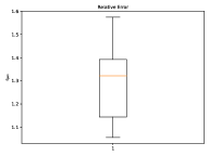
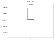
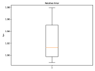
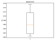
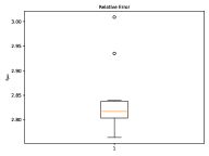
Error metrics: We present results in terms of the relative generalisation error (see e.g. Schobi et al. (2015); Lataniotis et al. (2020)) on the test data (about $10\%$ of all data) denoted by $\mathcal{T}$, given by:

$$\epsilon_{gen}=\frac{\sum_{i=1}^{|\mathcal{T}|}(y_{i}-\mu_{\tilde{y}_{i}})^{2}}{\sum_{i=1}^{|\mathcal{T}|}(y_{i}-\mu_{y})^{2}},$$ (13)

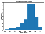
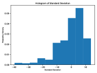
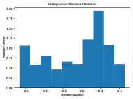
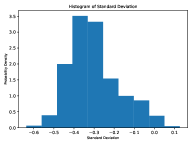
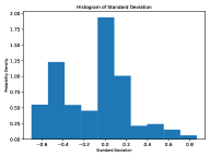
where $\mu_{y}$ is the mean of the true outputs of the test set, and $\mu_{\tilde{y}_{i}}$ is the PCE response mean approximately estimated using Monte-Carlo integration with 1000 samples. For each dataset, we performed 10 independent trials, and these are represented in the boxplots as follows. In the plots, the median error is represented using a central (orange) line and the top and bottom edges of the box are the 25th and 75th percentiles, respectively. Our results are comparable to other existing methods for supervised-learning, such as Least angle regression (LARS) Efron et al. (2004); Blatman and Sudret (2011). For each dataset, we compute the error using Eq. (13) for LARS (reported in the figure captions) and compare it to our results. For the PDE datasets, we achieve superior results over LARS, while for the other standard datasets the LARS outperforms by a small margin. In addition, for each test data-point, we measured the distance between the exact response and $\mu_{\tilde{y}_{i}}$ w.r.t the standard deviation $\sqrt{\text{Var}\left[\tilde{y}|{\mathbf{x}}_{i}\right]}$ as:

$$\frac{y_{i}-\mu_{\tilde{y}_{i}}}{\sqrt{\text{Var}\left[\tilde{y}|{\mathbf{x}}_{i}\right]}},\ i=1,\dots,|\mathcal{T}|\ .$$ (14)

We represent the probability density distribution of these results using the histogram plots. We can see in the histogram plots that our errors are distributed almost symmetrically around zero and most of the errors are within one standard deviation.

Figure 2: Left to Right: Boston housing, Parkinson Speech, Diabetes. Top: Histogram plot of the standard deviation. Bottom: box plots of the relative errors. LARS test errors: $0.2453,61598.57,0.5351$.

4.1 Machine Learning Datasets

We first demonstrate the performance of PCE-Net on three datasets that appear in machine learning applications, and are used for analyzing supervised-learning methods.

4.1.1 Boston Housing

This dataset concerns with the housing values in the suburbs of Boston, 1970. It was published in Harrison Jr and Rubinfeld (1978) and has been used in many machine learning articles that address regression problems, including analysis with different supervised learning methods in Quinlan (1993). The data consists of 506 samples with 13 features. The 13 features were encoded with a VAE (6 neurons in the hidden layer) into a 3-dimensional latent space. The learning rate was $10^{-4}$ and the number of epochs was $100$. For the PCE stage, we chose adaptively the degree to be 3. Results are reported in Figure 2 (left).

4.1.2 Parkinson Speech Dataset

The Parkinson dataset consists of 20 People with Parkinson’s and 20 healthy people who appeared at the Department of Neurology in Cerrahpasa Faculty of Medicine, Istanbul University. From all the patients, 26 types of sound recordings (voice samples including sustained vowels, numbers, words and short sentences) were taken and used as the features (1040 samples overall). UPDRS (Unified Parkinson Disease Rating Scale) score of each patient is the output which is determined by an expert physician. This dataset was collected and studied in Sakar et al. (2013). The 26 features were encoded with a VAE (12 neurons in the hidden layer) to a 4-dimensional latent space. The learning rate was $0.01$ and the number of epochs was $100$. For the PCE stage, we chose adaptively the degree to be 2. Results are reported in Figure 2 (center).

4.1.3 Diabetes Dataset

The diabetes dataset consists of 442 diabetes patients, with baseline of ten health features as well as the response of interest, a quantitative measure of disease progression one year after baseline. This dataset was analysed in Efron et al. (2004). The 10 features were encoded with a VAE (6 neurons in the hidden layer) to a 2-dimensional latent space. The learning rate was $10^{-3}$ and the number of epochs was $300$. For the PCE stage, we chose adaptively the degree to be 3. Results are reported in Figure 2 (right).

Figure 3: Left to Right: Allen-Cahn, Hamilton-Jacobi-Bellman. Top: Histogram plot of the standard deviation. Bottom: Box plot of the relative errors. LARS test error: $71054.25,8.8054$.

4.2 Learning Differential Equations

Next, we demonstrate how PCE-Net performs on problems that aim to learn solutions of PDEs. Both PDEs that are considered here appeared in Han et al. (2018) as examples for solving high-dimensional PDEs using deep learning.

4.2.1 Allen-Cahn Equation

We considered the following Allen-Cahn equation for $t\in[0,0.3]$ and ${\mathbf{x}}\in\mathbb{R}^{100}$:

$$\frac{\partial u}{\partial t}(t,{\mathbf{x}}) =\Delta u(t,{\mathbf{x}})+u(t,{\mathbf{x}})-u^{3}(t,{\mathbf{x}})$$

$$u(t=0.3,{\mathbf{x}}) =\frac{1}{2+0.4\|{\mathbf{x}}\|^{2}}\,.$$

We sampled ${\mathbf{x}}_{1},\dots,{\mathbf{x}}_{831}$ from different normal distributions, and used the method in Han et al. (2018) to obtain the solution $u(t=0,{\mathbf{x}}_{1}),\dots,u(t=0,{\mathbf{x}}_{831})$ for the equation. The goal of PCE-Net is to learn the input-output relation $({\mathbf{x}}_{1},u(t=0,{\mathbf{x}}_{1})),\dots,({\mathbf{x}}_{n},u(t=0,{\mathbf{x}}_{831}))$. The 100 features were encoded with a VAE (25 neurons in the hidden layer) to a 6-dimensional latent space. The learning rate was $10^{-5}$ and the number of epochs was $150$. For the PCE stage, we chose adaptively the degree to be 2. Results are reported in Figure 3 (left).

4.2.2 Hamilton-Jacobi-Bellman Equation

Lastly, we considered the following Hamilton-Jacobi-Bellman equation for $t\in[0,1]$ and ${\mathbf{x}}\in\mathbb{R}^{100}$:

$$\frac{\partial u}{\partial t}(t,{\mathbf{x}}) +\Delta u(t,x)-\|\nabla u(t,{\mathbf{x}})\|^{2}=0$$

$$u(t=1,{\mathbf{x}}) =\ln\left(\frac{1+\|{\mathbf{x}}\|^{2}}{2}\right)\,.$$

As in the example of Allen-Cahn equation, we sampled ${\mathbf{x}}_{1},\dots,{\mathbf{x}}_{1136}$ from different normal distributions, and used the method in Han et al. (2018) to obtain $u(t=0,{\mathbf{x}}_{1}),\dots,u(t=0,{\mathbf{x}}_{1136})$ from the equation. The goal of PCE-Net is to learn the input-output relations $({\mathbf{x}}_{1},u(t=0,{\mathbf{x}}_{1})),\dots,({\mathbf{x}}_{n},u(t=0,{\mathbf{x}}_{1136}))$. The 100 features were encoded with a VAE (16 neurons in the hidden layer) to a 6-dimensional latent space. The learning rate was $10^{-4}$ and the number of epochs was $150$. For the PCE stage, we chose adaptively the degree to be 2. Results are reported in Figure 3 (right).

5 Conclusions

In this paper, we presented PCE-Net, a surrogate model based approach for learning uncertainty in high-dimensional data systems. The method comprises of two stages; namely, a dimensionality reduction stage, where VAE is used to learn a distribution of the inputs on a low-dimensional latent space, and a surrogate modeling stage, where PCE and MMD are used to learn a mapping from the latent space to the output space. The combination of VAE and PCE provides means to learn a functional relation between the input and output distribution and also allows for uncertainty propagation. While the VAE ensures that the posterior distribution in the latent space captures the input distribution, PCE and MMD ratify that the global and conditional moments of the response match that of the outputs. In order to estimate the posterior statistics and moments it is only necessary to sample the latent space (rather than the high-dimensional input space itself), and henceforth the PCE captures the global characteristics of the data. Numerical experimental results on various datasets illustrate the utilities of the proposed method in different applications. PCE-Net yields reasonably accurate results for supervised learning, which are comparable to standard regression techniques. It can also model uncertainty in stochastic PDEs and learning problems.

References

- Abdar et al. [2021] M. Abdar, F. Pourpanah, S. Hussain, D. Rezazadegan, L. Liu, M. Ghavamzadeh, P. Fieguth, X. Cao, A. Khosravi, U. R. Acharya, et al. A review of uncertainty quantification in deep learning: Techniques, applications and challenges. Information Fusion, 2021.
- Bingham et al. [2019] E. Bingham, J. P. Chen, M. Jankowiak, F. Obermeyer, N. Pradhan, T. Karaletsos, R. Singh, P. Szerlip, P. Horsfall, and N. D. Goodman. Pyro: Deep universal probabilistic programming. The Journal of Machine Learning Research, 20(1):973–978, 2019.
- Blatman and Sudret [2011] G. Blatman and B. Sudret. Adaptive sparse polynomial chaos expansion based on least angle regression. Journal of computational Physics, 230(6):2345–2367, 2011.
- Böhm et al. [2019] V. Böhm, F. Lanusse, and U. Seljak. Uncertainty quantification with generative models. arXiv preprint arXiv:1910.10046, 2019.
- Chen et al. [2015] P. Chen, N. Zabaras, and I. Bilionis. Uncertainty propagation using infinite mixture of gaussian processes and variational bayesian inference. Journal of computational physics, 284:291–333, 2015.
- Chen et al. [2021] T. Chen, T. Trogdon, and S. Ubaru. Analysis of stochastic lanczos quadrature for spectrum approximation. arXiv preprint arXiv:2105.06595, 2021.
- Constantine et al. [2015] P. G. Constantine, M. Emory, J. Larsson, and G. Iaccarino. Exploiting active subspaces to quantify uncertainty in the numerical simulation of the hyshot ii scramjet. Journal of Computational Physics, 302:1–20, 2015.
- Crestaux et al. [2009] T. Crestaux, O. Le Maıtre, and J.-M. Martinez. Polynomial chaos expansion for sensitivity analysis. Reliability Engineering & System Safety, 94(7):1161–1172, 2009.
- Deng and Liu [2018] L. Deng and Y. Liu. Deep learning in natural language processing. Springer, 2018.
- Duong et al. [2016] P. L. T. Duong, T. N. Pham, J. Goncalves, E. Kwok, M. Lee, et al. Uncertainty quantification and global sensitivity analysis of complex chemical processes with a large number of input parameters using compressive polynomial chaos. Chemical Engineering Research and Design, 115:204–213, 2016.
- Efron et al. [2004] B. Efron, T. Hastie, I. Johnstone, and R. Tibshirani. Least angle regression. The Annals of statistics, 32(2):407–499, 2004.
- Fadlullah et al. [2017] Z. M. Fadlullah, F. Tang, B. Mao, N. Kato, O. Akashi, T. Inoue, and K. Mizutani. State-of-the-art deep learning: Evolving machine intelligence toward tomorrow’s intelligent network traffic control systems. IEEE Communications Surveys & Tutorials, 19(4):2432–2455, 2017.
- Feinberg and Langtangen [2015] J. Feinberg and H. P. Langtangen. Chaospy: An open source tool for designing methods of uncertainty quantification. Journal of Computational Science, 11:46–57, 2015.
- Ghanem and Spanos [1990] R. Ghanem and P. D. Spanos. Polynomial chaos in stochastic finite elements. 1990.
- Ghanem and Spanos [2003] R. G. Ghanem and P. D. Spanos. Stochastic finite elements: a spectral approach. Courier Corporation, 2003.
- Goodfellow et al. [2016] I. Goodfellow, Y. Bengio, and A. Courville. Deep learning. MIT press, 2016.
- Gretton et al. [2012] A. Gretton, K. M. Borgwardt, M. J. Rasch, B. Schölkopf, and A. Smola. A kernel two-sample test. The Journal of Machine Learning Research, 13(1):723–773, 2012.
- Guo et al. [2020] F. Guo, R. Xie, and B. Huang. A deep learning just-in-time modeling approach for soft sensor based on variational autoencoder. Chemometrics and Intelligent Laboratory Systems, 197:103922, 2020.
- Han et al. [2018] J. Han, A. Jentzen, and E. Weinan. Solving high-dimensional partial differential equations using deep learning. Proceedings of the National Academy of Sciences, 115(34):8505–8510, 2018.
- Harrison Jr and Rubinfeld [1978] D. Harrison Jr and D. L. Rubinfeld. Hedonic housing prices and the demand for clean air. Journal of environmental economics and management, 5(1):81–102, 1978.
- Hinton and Van Camp [1993] G. E. Hinton and D. Van Camp. Keeping the neural networks simple by minimizing the description length of the weights. In Proceedings of the sixth annual conference on Computational learning theory, pages 5–13, 1993.
- Jordan et al. [1998] M. I. Jordan, Z. Ghahramani, T. S. Jaakkola, and L. K. Saul. An introduction to variational methods for graphical models. In Learning in graphical models, pages 105–161. Springer, 1998.
- Kiasari et al. [2017] M. A. Kiasari, D. S. Moirangthem, and M. Lee. Generative moment matching autoencoder with perceptual loss. In International Conference on Neural Information Processing, pages 226–234. Springer, 2017.
- Kingma and Welling [2013] D. P. Kingma and M. Welling. Auto-encoding variational bayes. arXiv preprint arXiv:1312.6114, 2013.
- Lataniotis et al. [2020] C. Lataniotis, S. Marelli, and B. Sudret. Extending classical surrogate modeling to high dimensions through supervised dimensionality reduction: a data-driven approach. International Journal for Uncertainty Quantification, 10(1), 2020.
- Li et al. [2006] H.-s. Li, Z.-z. Lü, and Z.-f. Yue. Support vector machine for structural reliability analysis. Applied Mathematics and Mechanics, 27(10):1295–1303, 2006.
- Li et al. [2015] Y. Li, K. Swersky, and R. Zemel. Generative moment matching networks. In International Conference on Machine Learning, pages 1718–1727. PMLR, 2015.
- Ma and Zabaras [2011] X. Ma and N. Zabaras. Kernel principal component analysis for stochastic input model generation. Journal of Computational Physics, 230(19):7311–7331, 2011.
- Malinin [2019] A. Malinin. Uncertainty estimation in deep learning with application to spoken language assessment. PhD thesis, University of Cambridge, 2019.
- Mehrasa et al. [2019] N. Mehrasa, A. A. Jyothi, T. Durand, J. He, L. Sigal, and G. Mori. A variational auto-encoder model for stochastic point processes. In Proceedings of the IEEE/CVF Conference on Computer Vision and Pattern Recognition, pages 3165–3174, 2019.
- Mohamed et al. [2010] L. Mohamed, M. Christie, and V. Demyanov. Comparison of stochastic sampling algorithms for uncertainty quantification. SPE Journal, 15(01):31–38, 2010.
- Najm [2009] H. N. Najm. Uncertainty quantification and polynomial chaos techniques in computational fluid dynamics. Annual review of fluid mechanics, 41:35–52, 2009.
- Oladyshkin and Nowak [2012] S. Oladyshkin and W. Nowak. Data-driven uncertainty quantification using the arbitrary polynomial chaos expansion. Reliability Engineering & System Safety, 106:179–190, 2012.
- Quinlan [1993] J. R. Quinlan. Combining instance-based and model-based learning. In Proceedings of the tenth international conference on machine learning, pages 236–243, 1993.
- Rasmussen [2003] C. E. Rasmussen. Gaussian processes in machine learning. In Summer school on machine learning, pages 63–71. Springer, 2003.
- Sakar et al. [2013] B. E. Sakar, M. E. Isenkul, C. O. Sakar, A. Sertbas, F. Gurgen, S. Delil, H. Apaydin, and O. Kursun. Collection and analysis of a parkinson speech dataset with multiple types of sound recordings. IEEE Journal of Biomedical and Health Informatics, 17(4):828–834, 2013.
- Schobi et al. [2015] R. Schobi, B. Sudret, and J. Wiart. Polynomial-chaos-based kriging. International Journal for Uncertainty Quantification, 5(2), 2015.
- Sepahvand et al. [2010] K. Sepahvand, S. Marburg, and H.-J. Hardtke. Uncertainty quantification in stochastic systems using polynomial chaos expansion. International Journal of Applied Mechanics, 2(02):305–353, 2010.
- Smith [2013] R. C. Smith. Uncertainty quantification: theory, implementation, and applications, volume 12. Siam, 2013.
- Soize and Ghanem [2004] C. Soize and R. Ghanem. Physical systems with random uncertainties: chaos representations with arbitrary probability measure. SIAM Journal on Scientific Computing, 26(2):395–410, 2004.
- Sullivan [2015] T. J. Sullivan. Introduction to uncertainty quantification, volume 63. Springer, 2015.
- Torre et al. [2019] E. Torre, S. Marelli, P. Embrechts, and B. Sudret. Data-driven polynomial chaos expansion for machine learning regression. Journal of Computational Physics, 388:601–623, 2019.
- Tripathy et al. [2016] R. Tripathy, I. Bilionis, and M. Gonzalez. Gaussian processes with built-in dimensionality reduction: Applications to high-dimensional uncertainty propagation. Journal of Computational Physics, 321:191–223, 2016.
- Tripathy and Bilionis [2018] R. K. Tripathy and I. Bilionis. Deep uq: Learning deep neural network surrogate models for high dimensional uncertainty quantification. Journal of computational physics, 375:565–588, 2018.
- Ubaru et al. [2021] S. Ubaru, L. Horesh, and G. Cohen. Dynamic graph and polynomial chaos based models for contact tracing data analysis and optimal testing prescription. Journal of biomedical informatics, 122:103901, 2021.
- Verleysen and Francois [2005] M. Verleysen and D. Francois. The curse of dimensionality in data mining and time series prediction. In International work-conference on artificial neural networks, pages 758–770. Springer, 2005.
- Voulodimos et al. [2018] A. Voulodimos, N. Doulamis, A. Doulamis, and E. Protopapadakis. Deep learning for computer vision: A brief review. Computational intelligence and neuroscience, 2018, 2018.
- Wang and Yeung [2016] H. Wang and D.-Y. Yeung. Towards bayesian deep learning: A framework and some existing methods. IEEE Transactions on Knowledge and Data Engineering, 28(12):3395–3408, 2016.
- Waterhouse et al. [1996] S. Waterhouse, D. MacKay, T. Robinson, et al. Bayesian methods for mixtures of experts. Advances in neural information processing systems, pages 351–357, 1996.
- Wilson and Izmailov [2020] A. G. Wilson and P. Izmailov. Bayesian deep learning and a probabilistic perspective of generalization. arXiv preprint arXiv:2002.08791, 2020.
- Xiu and Karniadakis [2002] D. Xiu and G. E. Karniadakis. The wiener–askey polynomial chaos for stochastic differential equations. SIAM journal on scientific computing, 24(2):619–644, 2002.
- Zhang et al. [2019] D. Zhang, L. Lu, L. Guo, and G. E. Karniadakis. Quantifying total uncertainty in physics-informed neural networks for solving forward and inverse stochastic problems. Journal of Computational Physics, 397:108850, 2019.
- Zheng et al. [2021] X. Zheng, J. Zhang, N. Wang, G. Tang, and W. Yao. Mini-data-driven deep arbitrary polynomial chaos expansion for uncertainty quantification. arXiv preprint arXiv:2107.10428, 2021.