Elucidating the $\rho$-meson’s role as intermediate resonance in the time-like electromagnetic pion form factor

Abstract

Motivated by the planned measurements of the time-like electromagnetic proton form factors an exploratory study of the time-like electromagnetic pion form factor is presented in a formalism which describes mesons as Poincaré-invariant bound states. In the respective quark interaction kernel, beyond the gluon-intermediated interactions for valence-type quarks, non-valence effects are included by allowing the pions to couple back in a self-consistent manner to the quarks. Consequently, the opening of the dominant $\rho$ decay channel, $\rho\to\pi\pi$, and the presence of a multi-particle branch cut, setting in when the two-pion threshold is crossed, are included consistently, first in the correspondingly calculated quark-photon vertex, and then consequently in the time-like electromagnetic pion form factor. The obtained results are in agreement with the available experimental data and provide further evidence for the efficacy of a vector-meson dominance model. Effects of going beyond the here employed isospin-symmetric limit are discussed. Last but not least, an outlook is provided on how to include in Poincaré-covariant Faddeev approaches the effects of intermediate resonances in the calculation of baryon properties.

1 Introduction

Quantum Chromodynamics (QCD) provides the basis for our current understanding of hadron physics. Perturbative as well as non-perturbative QCD calculations have become impressively successful in the last decades. From a theoretical point of view, QCD is a model Quantum Field Theory. It realises locality and unitarity, and being asymptotically free QCD is an ultraviolet complete Quantum Field Theory. The latter property quite obviously underlies the success of perturbative calculations for hard hadronic and semi-hadronic processes.

The perturbative description of elementary particles is essentially based on the field-particle duality which means that each field in a Quantum Field Theory is associated with a physical particle. Quite obviously, this is not the case for the elementary fields of QCD, the quarks and gluons. First of all, QCD being a gauge theory, together with the fact that only gauge-invariant quantities can be observables, rules already out that quarks and gluons can be directly observed. In a gauge theory, the rôle of fields is to implement the principle of locality. The types of different elementary fields needed in the theory is related to the structure of the gauge group, it is not, at least not directly, related to the empirical spectrum of particles. Second, what is usually referred to as “confinement” is obviously going beyond the mere issue of “only-gauge-invariant-observables”, respectively, colour confinement (see, e.g., refs. Greensite:2011zz ; Alkofer:2006fu ), and an especially puzzling aspect is the following: As only hadrons are produced from processes involving hadronic initial states, one has to explain that the only thresholds in hadronic amplitudes are due to the productions of other hadronic states. Consequently, singularities occurring in the amplitudes of hadronic and thus composite states are exclusively due to their hadronic substructure, or phrased otherwise, due to virtual fluctuations to hadronic resonances.

This implies not only that hadron spectroscopy and hadron structure are strongly interrelated, but, in particular, that a microscopic understanding of the effect of resonances on form factors, structure functions, etc., will shed light on the precise working of quark-hadron duality. Compelling evidence for the consequences of this duality on the qualitative as well as the semi-quantitative level has been found (for a review see, e.g., Ref. Melnitchouk:2005zr ) and contributed to a verification of this duality which is, beyond the trivial fact of the absence of coloured states, the clearest experimental signature for confinement. The attributed perfect orthogonality of the quark and gluon degrees of freedom on the one hand and hadronic states on the other hand, and thus the perfect absence of ââdouble-countingââ when doing calculations either with quarks and gluons within QCD or within purely hadronic descriptions, is nothing else but another way to express central aspects of confinement. Basing a (confessedly impossible) exact calculation for a hadronic or semi-hadronic scattering process either on elementary QCD correlation functions or only on hadronic correlations functions needs to lead to the same result by the virtue of colour confinement, the latter being a consequence of gauge invariance. The way by which the hadronic amplitudes become effectively independent of the singularities of the elementary correlation functions is then an imprint of the dynamical realisation of confinement.

The formation of an excited hadronic bound state, being an unstable resonance, is closely related to the open decay channels. This is most evident from the analysis of time-like form factors in kinematic regions close to a resonance. To capture this interplay correctly in a QCD-based calculation of a hadron form factor, the in- (respectively, out-) going hadron and the hadronic resonance which is apparent in the form factor have to be described both in a mutual consistent manner as composite objects of quarks and gluons. Thus, a calculation of a time-like form factor from QCD, or from a microscopic model based on QCD degrees of freedom, has to overcome the challenge to treat all necessary elements on the same basis and to a sufficient degree of sophistication. Only then the result will allow conclusions on the hadron structure encoded in such a form factor.

It should be emphasised that the presented study aims for comprehending the interplay of the different features of the form factor and as they arise from the QCD degrees of freedom. It is also designed such that it can be generalised to an investigation of baryon form factors, and hereby especially the nucleons’ time-like form factor. (NB: Different space-like baryon form factors have been calculated in this approach, see, e.g., Refs. Eichmann:2016yit ; Nicmorus:2010sd ; Eichmann:2011vu ; Eichmann:2011pv ; Sanchis-Alepuz:2013iia ; Sanchis-Alepuz:2017mir for some recent respective work.) A thorough understanding of the proton time-like form factor at very low $Q^{2}$ is a very timely subject as the upcoming PANDA experiment possesses the unique possibility to measure the proton’s electromagnetic form factors in the so-called unphysical region through the process $\bar{p}p\to l^{+}l^{-}\pi^{0}$, $l=e,\mu$ Fischer:2021kcr . At large $Q^{2}$ the question of the onset of the convergence scale between the space-like and the time-like form factors arises.

In this talk an exploratory study of the time-like pion electromagnetic form factor employing a combination of Bethe-Salpeter and Dyson-Schwinger equations Miramontes:2021xgn will be discussed, and its results will be presented. To obtain the most important features of the pions’ time-like form factor one needs to take into account
(i) the pion as bound state of quark and antiquark thereby at the same accommodating its special role as would-be Goldstone boson of the dynamically broken chiral symmetry of QCD,
(ii) the mixing of the $\rho$-meson, being determined consistently as a quark-antiquark bound state, with a virtual photon when this photon is in turn coupled to a quark-antiquark pair via the fully renormalised quark-photon vertex, and
(iii) the dominant decay channel of the $\rho$-meson, namely, $\rho\to\pi\pi$.

Before presenting how to combine these in our study a few general remarks about the time-like pion electromagnetic form factor are in order.

2 The time-like electromagnetic pion form factor: General aspects

Figure 1: Electron-positron pair annihilating to a virtual photon with time-like momentum which then decays to a pion pair.

Experimentally the time-like electromagnetic pion form factor is typically determined from electron-positron pair annihilation into a pion pair, see Fig. 1. In the physical region above the two-pion production threshold the corresponding amplitude possesses a cut, and thus the time-like pion form factor has to be treated as a complex quantity.

The pion form factor contains all kind of processes turning a virtual photon into a pion pair, cf. Fig.  1. Using that in the interesting kinematic regime strong-interaction processes dominate by orders of magnitude against electroweak processes, an important first ingredient to the pion form factor is how the virtual photon couples to a quark via all possible QCD processes. The corresponding amplitude is nothing else than the full quark-photon vertex which includes, at least in principle, the information about the virtual photon’s hadronic substructure. The two more further ingredients are the quark propagator and the pion bound state amplitude.

The presented study is performed in the isospin symmetric limit. As isospin breaking is clearly visible in the time-like pion form factor, in particular through $\rho$-$\omega$ mixing, a vector meson dominance (VMD) based fit is used to extract the expected form of the pion form factor without this mixing effect, see Fig. 2.

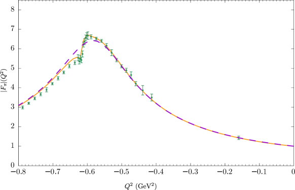
Figure 2: Absolute value of the pion form factor in the time-like ($Q^{2}<0$) domain from the VMD-based fit given in ref. OConnell:1995nse (full line) in comparison to the experimental data Akhmetshin:2006bx . The dashed line is based on the same expression but without $\rho$-$\omega$ mixing, i.e., the mixing matrix element is put to zero.

As can be seen from Fig. 2 the VMD model of ref. OConnell:1995nse describe the experimental data precisely. But how does it arise from the dynamics of QCD degrees of freedom?

3 Interactions in Dyson-Schwinger and Bethe-Salpeter equations

The interactions used in the exploratory study Miramontes:2021xgn have been a gluon exchange (in the form of the Maris-Tandy model Maris:1997tm ; Maris:1999nt ) as well as a pion exchange and $s$- and $u$-channel pion decay contributions, see Fig. 3, the latter both in self-consistent manner. Here the following disclaimer is in order: To keep this calculation feasible a number of technically motivated approximations have been made. It has been checked that these had only a minor impact on the results, for further details see Ref. Miramontes:2021xgn .

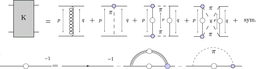
Figure 3: Truncations used herein for the Bethe-Salpeter interaction kernel $K$ (upper diagram) and the quark Dyson-Schwinger equation (lower diagram). In the upper diagram, the terms on the right-hand side correspond to the gluon, pion exchange, and s- and u-channel pion decay contributions to the truncation, respectively. The s- and u-channel pion decay terms do not contribute to the quark Dyson-Schwinger equation.

As already stated the quark-photon vertex is a decisive element in the presented calculation. It has been determined with the above mentioned interactions in Ref. Miramontes:2019mco . The Dirac structure of the vertex can be expanded in a basis consisting of twelve elements, and all of them are taken into account to obtain the below displayed results. In addition, out of these twelve structure eight are transverse to the photon’s momentum. These transverse amplitudes display a pole at the (calculated) $\rho$-meson mass and multi-pion cut above the two-pion threshold.

The Dyson-Schwinger and Bethe-Salpeter equations are integral equations which are solved numerically. Hereby, for the presented calculation the major technical challenge arises from the singularities of the integrands. This implies that one has to find integration contours in presence of cuts generated by quark propagator poles and the pion propagator pole as well as two-pion cuts and the $\rho$ pole, the latter two also arising in the quark-photon vertex. To this end one has to determine, typically by resolving respective conditions numerically, the location of poles and cuts of the integrand. Then the integration contour is deformed such no cuts are crossed and no residues of poles are inadvertently picked up. Fig. 4 shows an example of such a contour deformation. Note that different contour deformations have to be done for different external momenta.

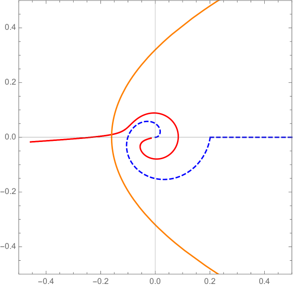
Figure 4: Shown is the complex $p^{2}$ plane such that time-like momenta correspond to the left real half-axis. Without singularities in the integrand the integration would be performed over space-like momenta, i.e., over the right real half-axis. In the presented example this is not possible due to the pion cut represented by the red fill line. Correspondingly, the integration contour is deformed to the dashed blue line. The singularities of the quark propagator are all to the left of the displayed parabola, and therefore do not necessitate further contour deformations.

4 Results

For the presented exploratory calculation, the parameters are adjusted in a simple manner, especially as we aim at a qualitative understanding of the physical mechanisms involved in determining the shape of the pion form factor, and not so much at achieving an accurate quantitative agreement with experiment. As the pion-decay kernels will not only move the $\rho$-meson pole into the complex plane but also shift down its real value a precise fit of the two (effective) parameters of the Maris-Tandy model to reproduce the meson masses would have required quite some computational resources. In addition, only a reasonably accurate value for the pion decay constant, namely $f_{\pi}$= 138 MeV has resulted. Although this value is a few percent larger than the experimental one, $f^{expt.}_{\pi}=130.5$ MeV, we have adopted it in view of a compromise in the effort needed for the parameter determination and the related accuracy. In table 1 the determined meson masses as well as the pion decay constant are shown.

Table 1: The pion mass $m_{\pi}$, the pion decay constant $f_{\pi}$, the $\rho$-meson and $\omega$-meson masses $m_{\rho}$ and $m_{\omega}$ for the two different used parameterisations of the model (labeled with $\eta$) and for the case with gluon- and pion-exchange kernels but without decay kernels are shown. The current quark mass has been set to $m_{q}=6.8\leavevmode\nobreak\$MeV. The two rightmost, separated, columns display for the case when including the decay kernels the extracted $\rho$-meson pole position defined as $M_{pole}^{2}=M_{\rho}^{2}-iM_{\rho}\Gamma_{\rho}$. All values for dimensionful quantities are given in GeV.

$\Lambda=0.78$	$m_{\pi}$	$f_{\pi}$	$m_{\rho}$	$m_{\omega}$	$M_{\rho}$	$\Gamma_{\rho}$
$\eta=1.5$	0.139	0.138	0.768	0.778	0.750	0.100
$\eta=1.6$	0.126	0.138	0.774	0.784	0.759	0.105

The pion exchange kernels lift the otherwise present degeneracy in between the iso-vector $\rho$- and the iso-singlet $\omega$-meson. These interactions induce a mass splitting $m_{\omega}-m_{\rho}=10$ MeV which compares favourably with the experimental splitting of 7 - 8 MeV.

Fig. 5 displays our results for the space-like form factor from which we also extract the result for the pion radius, $\sqrt{\langle r_{\pi}^{2}\rangle}=$ 0.68 fm. It is reassuring that the space-like form factor, including the pion radius, shows a very good agreement with experimental data. As we included the most important physical processes with effects in the time-like regime we take this as evidence that the imaginary part in the time-like region is precisely enough reproduced to provide very good results for the space-like form factor.

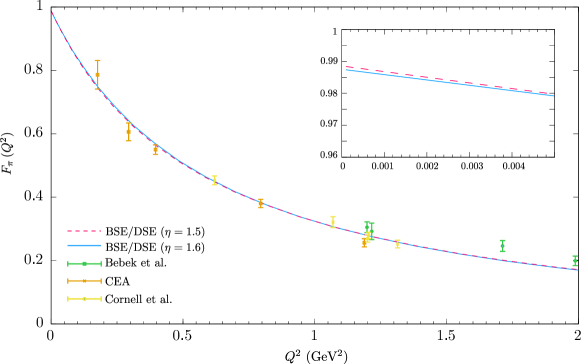
Figure 5: Pion form factor in the spacelike $Q^{2}>0$ domain for the model parameters $\eta=1.5$ and $\eta=1.6$. (The inset illustrates the impact of one of the technically motivated approximations.)

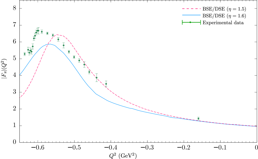
Figure 6: Absolute value of the pion form factor in the time-like $Q^{2}<0$ domain for the model parameters $\eta=1.5$ and $\eta=1.6$ as described in the text and compared to experimental data Akhmetshin:2006bx .

The results for the absolute value of the pion form factor for time-like ($Q^{2}<0$) virtualities are displayed in Figs. 6. As a consequence of the decay kernels, the pion form factor (as well as the quark-photon vertex) possess a cut along the real negative axis starting at the two-pion threshold $Q^{2}=-4m_{\pi}^{2}$, and therefore also an imaginary part contributes significantly to the absolute value.

With decay kernels included, the $\rho$-meson pole, present in the quark-photon vertex, moves into the complex plane, and consequently the pion form factor develops a bump-like shape with approximately correct height and width. Therefore the presented calculation corrects a deficiency of earlier respective studies of the time-like pion form factor, without or even with the pion exchange term, for which the form factor diverges at the $Q^{2}$-value corresponding to the $\rho$-meson mass.

Table 2: The coefficients of the rational fits to the pion form factor as discussed in the text. All values for dimensionful quantities are given in GeV.

	$\eta$ =1.5	$\eta$ =1.6	VMD expression		$\eta$ =1.5	$\eta$ =1.6	VMD expression
$a_{1}$	0.5587	0.4149	0.72	$c_{1}$	0.0591	0.0997	0
$a_{2}$	0.8828	0.6827	1.2	$c_{2}$	0.1295	0.2383	0.2308
$b_{0}$	0.3600	0.3600	0.36	$d_{0}$	0.3600	0.3600	0.36
$b_{1}$	1.2307	1.2517	1.2	$d_{1}$	1.1924	1.2464	1.2
$b_{2}$	1.0722	1.1000	1.037	$d_{2}$	0.9973	1.0916	1.037

In order to provide a measure for the proximity of our results to the VMD predictions we performed rational fits (Padé fits) to the results for the real part and for the imaginary part of the form factor and compare the coefficients to the VMD expression without $\rho$-$\omega$ mixing. To stay as general as possible we used first an ansatz with twelve parameters in total:

$$Re\,F_{\pi}(Q^{2})-F_{\pi}(0) \approx -\frac{a_{0}+a_{1}Q^{2}+a_{2}(Q^{2})^{2}+a_{3}(Q^{2})^{3}}{b_{0}+b_{1}Q^{2}+b_{2}(Q^{2})^{2}+b_{3}(Q^{2})^{3}}$$

$$Im\,F_{\pi}(Q^{2}) \approx \frac{c_{0}+c_{1}Q^{2}+c_{2}(Q^{2})^{2}+c_{3}(Q^{2})^{3}}{d_{0}+d_{1}Q^{2}+d_{2}(Q^{2})^{2}+d_{3}(Q^{2})^{3}}\,.$$

We obtained almost vanishing values for the coefficients $a_{0}$, $a_{3}$, $b_{3}$, $c_{0}$, $c_{3}$ and $d_{3}$. Phrased otherwise, the fit confirms the structure expected from the VMD expression. Based on this, the fits have been repeated for

$$Re\,F_{\pi}(Q^{2})-F_{\pi}(0) \approx -\frac{a_{1}Q^{2}+a_{2}(Q^{2})^{2}}{b_{0}+b_{1}Q^{2}+b_{2}(Q^{2})^{2}}\,,$$

$$\quad Im\,F_{\pi}(Q^{2}) \approx \frac{c_{1}Q^{2}+c_{2}(Q^{2})^{2}}{d_{0}+d_{1}Q^{2}+d_{2}(Q^{2})^{2}}\,.$$ (2)

The coefficients resulting from these fitting ansätze as well as the ones resulting from VMD expression are given in table 2. Note that the expression based on the VMD hypothesis is an astonishingly good representation of the results based on the microscopic model of QCD degrees of freedom: Other terms than VMD-predicted ones are tiny, and the elaborated calculation yields within error margin the VMD predicted functional form.

Another remark applies to the fact that there is no significant impact from quark propagator poles on the pion form factor. As discussed in the Introduction this is a wanted feature in the view of confinement, however, it should be understood why this happens in the presented study which contains, despite its quite high level of sophistication, not all QCD features.

Reassuring is nevertheless that the resulting time-like pion form factor in the kinematic region $0>Q^{2}>0.8$GeV² is determined by the $\rho$-meson pole and the two-pion cut despite basing the calculation on QCD degrees of freedom.

5 Conclusions and Outlook

The main message of the presented study is the feasibility of studying time-like quantities in a Dyson-Schwinger–Bethe-Salpeter approach including intermediate resonances and thus decay channels in the interaction kernels. Despite the applied modelling (which can be overcome in future investigations) and the technical limitations inherent to the approach we found a remarkable agreement with the experimental data.

As a side result we provided a detailed quantitative verification of the VMD model for the pion form factor. In view of the fact that the $\rho$-meson pole and the two-pion cut are determining the prominent features of the pion form factor it might be considered expected that the VMD hypothesis should be, at least, qualitatively correct. Therefore, the more surprising, and definitely positive, aspect is that a microscopic model built on QCD degrees of freedom provide a pion form factor shaped by the hadron substructure of the virtual photon.

One obvious way to improve the presented study is to take isospin breaking via the different quark masses and electric charges into account. First steps in this direction have been undertaken Miramontes:2022mex , however, a microscopic description for $\rho$-$\omega$-mixing including the decay channels for these vector mesons, and its implementation into a calculation of the pion form factor, is still a task to be performed yet.

It would be also worth to extend the presented study to calculate the $\gamma$ $\pi$ $\pi$ $\pi$ form factor which is only non-vanishing due to the chiral anomaly. How in such a form factor, whose soft-point value is fixed due to the anomaly and thus easily understood from the perspective of QCD, the hadron resonances are determining the prominent time-like features will be of general interest.

Last but not least, the question of the accessibility of the nucleons’ time-like form factors arises. The presented study paves the way for an analogous inclusion of decay kernels into baryon bound state equations. To this end we note that a functional approach based on Dyson-Schwinger and bound-state equations allows for a unified description of mesons and baryons, see, e.g., Ref. Eichmann:2016yit , which quite successfully describes the hadron spectrum and space-like form factors. However, exactly these studies provide an estimate about the dramatic increase in complexity when dealing with baryon instead of meson bound state equations and a respective calculation of form factors based on these equations. Nevertheless, given the increased effort from the experimental side and the resulting anticipated highly precise data over a large kinematical region certainly justifies the correspondingly increased effort on the theoretical side.

References

- (1) J. Greensite, An introduction to the confinement problem, Lect. Notes Phys. 972, 2nd ed., 2020.
- (2) R. Alkofer and J. Greensite, J. Phys. G 34 (2007) S3 [arXiv:hep-ph/0610365 [hep-ph]].
- (3) W. Melnitchouk, R. Ent and C. Keppel, Phys. Rept. 406 (2005) 127 [arXiv:hep-ph/0501217 [hep-ph]].
- (4) Á. Miramontes, H. Sanchis-Alepuz and R. Alkofer, Phys. Rev. D 103 (2021) 116006 [arXiv:2102.12541 [hep-ph]].
- (5) G. Eichmann, H. Sanchis-Alepuz, R. Williams, R. Alkofer and C. S. Fischer, Prog. Part. Nucl. Phys. 91 (2016) 1 [arXiv:1606.09602 [hep-ph]].
- (6) D. Nicmorus, G. Eichmann and R. Alkofer, Phys. Rev. D 82 (2010) 114017 [arXiv: 1008.3184 [hep-ph]].
- (7) G. Eichmann, Phys. Rev. D 84 (2011) 014014 [arXiv:1104.4505 [hep-ph]].
- (8) G. Eichmann and C. S. Fischer, Eur. Phys. J. A 48 (2012) 9 [arXiv:1111.2614 [hep-ph]].
- (9) H. Sanchis-Alepuz, R. Williams and R. Alkofer, Phys. Rev. D 87 (2013) 096015 [arXiv:1302.6048 [hep-ph]].
- (10) H. Sanchis-Alepuz, R. Alkofer and C. S. Fischer, Eur. Phys. J. A 54 (2018) 41 [arXiv:1707.08463 [hep-ph]].
- (11) G. Barucca et al. [PANDA], [arXiv:2101.11877 [hep-ex]].
- (12) B. Ananthanarayan, I. Caprini and D. Das, Phys. Rev. D 102 (2020) 096003 [arXiv: 2008.00669 [hep-ph]].
- (13) H. B. O’Connell, B. C. Pearce, A. W. Thomas and A. G. Williams, Prog. Part. Nucl. Phys. 39 (1997) 201 [arXiv:hep-ph/9501251 [hep-ph]].
- (14) R. R. Akhmetshin et al. [CMD-2], Phys. Lett. B 648 (2007) 28 [arXiv:hep-ex/0610021 [hep-ex]].
- (15) Á. S. Miramontes, R. Alkofer, C. S. Fischer and H. Sanchis-Alepuz, [arXiv:2202.04618 [hep-ph]].
- (16) P. Maris and C. D. Roberts, Phys. Rev. C 56 (1997) 3369 [nucl-th/9708029].
- (17) P. Maris and P. C. Tandy, Phys. Rev. C 60 (1999) 055214 [nucl-th/9905056].
- (18) Á. S. Miramontes and H. Sanchis-Alepuz, Eur. Phys. J. A 55 (2019) 170 [arXiv: 1906.06227 [hep-ph]].
- (19) Á. Miramontes, A. Bashir, K. Raya and P. Roig, arXiv:2112.13916 [hep-ph].