Differential Private Knowledge Transfer for Privacy-Preserving Cross-Domain Recommendation
Abstract.
Cross Domain Recommendation (CDR) has been popularly studied to alleviate the cold-start and data sparsity problem commonly existed in recommender systems. CDR models can improve the recommendation performance of a target domain by leveraging the data of other source domains. However, most existing CDR models assume information can directly ‘transfer across the bridge’, ignoring the privacy issues. To solve this problem, we propose a novel two stage based privacy-preserving CDR framework (PriCDR). In the first stage, we propose two methods, i.e., Johnson-Lindenstrauss Transform (JLT) and Sparse-aware JLT (SJLT), to publish the rating matrix of the source domain using Differential Privacy (DP). We theoretically analyze the privacy and utility of our proposed DP based rating publishing methods. In the second stage, we propose a novel heterogeneous CDR model (HeteroCDR), which uses deep auto-encoder and deep neural network to model the published source rating matrix and target rating matrix respectively. To this end, PriCDR can not only protect the data privacy of the source domain, but also alleviate the data sparsity of the source domain. We conduct experiments on two benchmark datasets and the results demonstrate the effectiveness of PriCDR and HeteroCDR.
1. Introduction
Cross-Domain Recommendation (CDR) has been popularly studied recently, due to its powerful ability to solve the data sparsity issue of traditional recommender systems (Zhu et al., 2021a). Most existing CDR models focus on leveraging different kinds of data across multiple domains to improve the recommendation performance of a target domain (or domains) through ‘bridges’. Here, the data are usually users’ private data, e.g., user-item rating, review, and user profile. The ‘bridge’ refers to the linked objects between different domains such as common user, common item, and common features.
Privacy issues in CDR. Existing CDR models assume information can directly ‘transfer across the bridge’, ignoring the privacy issues. The key of CDR model is designing transfer strategies across bridges, e.g., cross network (Hu et al., 2018) and dual transfer network (Li and Tuzhilin, 2020). The above models assume all data are plaintext to both domains, which is inconsistent with reality. Since these data for CDR models usually involve user sensitive information and cannot be shared with others due to regulation reasons. Therefore, how to build CDR models on the basis of protecting data privacy becomes an urgent research problem.
Problem definition. In this paper, we consider a two-domain cross recommendation problem for simplification. Specifically, we assume there are two domains (a source domain and a target domain) which have the same user set but different user-item interaction pairs. We also assume the user-item interactions only have rating data and leave other side-information as future work. The problem of privacy-preserving CDR is to improve the recommendation performance of the target domain by leveraging the data of the source domain, while protecting the data privacy of both domains.
Existing work. The existing privacy-preserving recommendation models are mainly designed for two categories, i.e., individual customers and business partners. The former assumes that each client only contains the private data of a single user (Nikolaenko et al., 2013; Hua et al., 2015; Chen et al., 2018), and the existing work on this either assumes the existence of a semi-honest server or reveals middle information (e.g., latent factors) during model training. The later assumes that each client (domain) has the private data of a batch of users (Ogunseyi et al., 2021; Gao et al., 2019b, a; Chen et al., 2020a; Cui et al., 2021), which can be seen as privacy-preserving CDR models. However, they are customized to certain settings, e.g., social recommendation (Chen et al., 2020a) and location recommendation (Gao et al., 2019b), and thus are not suitable to our problem.
Our proposal. In this paper, we propose a novel two stage based privacy-preserving CDR framework (PriCDR). In stage one, the source domain privately publishes its user-item ratings to the target domain. In stage two, the target domain builds a CDR model based on its raw data and the published data of the source domain.
Design goals. The two stages in PriCDR should have the following goals. First, for stage one, user-item rating matrix publishing should not only preserve the data privacy of the source domain, but also facilitate the following CDR task. Specifically, there should be the following requirements in rating publishing. (1) Privacy-preserving. From the published user-item ratings, the target domain should not identify whether a user has rated an item. (2) Restricted isometry property. The nature of most recommender systems is collaborative filtering. That is, users who have similar ratings tend to share similar tastes. Thus, the published rating matrix should approximate the original one well, as the restricted isometry property stated in the literature of matrix completion (Candes and Tao, 2005). Thus, the users can still collaborate with each other. (3) Sparse-awareness. Data sparsity is a long-standing problem in recommender systems. Thus, rating publishing should be able to handle the sparse user-item rating data. After rating publishing in stage one, the user-item rating data becomes heterogeneous in stage two. However, most existing CDR frameworks, e.g., (Zhu et al., 2019; Chen et al., 2020b; Yuan et al., 2019; Li and Tuzhilin, 2020; Hu et al., 2018), are symmetrical. Thus, a new CDR framework that can handle such heterogeneous data is needed.
Technical solution. In stage one, inspired by the fact that Johnson-Lindenstrauss Transform (JLT) preserves differential privacy (Blocki et al., 2012), we propose two methods to publish rating matrix differential privately. We first propose JLT based differential private rating matrix publishing mechanism, which can not only protect data privacy but also preserve the similarity between users. We then propose Sparse-aware JLT (SJLT) which can further reduce the computation complexity of JLT and alleviate the data sparsity in the source domain with sub-Gaussian random matrix and Hadamard transform. We finally theoretically analyze their privacy and utility. In stage two, we propose a novel heterogeneous CDR model (HeteroCDR), which uses deep auto-encoder and deep neural network to model the published source rating matrix and target rating matrix, respectively. We also propose an embedding alignment module to align the user embeddings learnt from two networks.
Contributions. We summarize our main contributions as follows: (1) We propose PriCDR, a general privacy-preserving CDR framework, which has two stages, i.e., rating publishing and cross-domain recommendation modeling. (2) We propose two differential private rating publishing algorithms, via JLT and SJLT respectively, we also provide their privacy and utility guarantees. (3) We propose HeteroCDR to handle the heterogeneous rating data between the published source domain and target domain. (4) We conduct experiments on two benchmark datasets and the results demonstrate the effectiveness of PriCDR and HeteroCDR.
2. Related Work
2.1. Cross Domain Recommendation
Cross Domain Recommendation (CDR) is proposed to handle the cold-start and data sparsity problem commonly existed in the traditional single domain recommender systems (Zhu et al., 2021a). The basic assumption of CDR is that different behavioral patterns from multiple domains jointly characterize the way users interact with items (Li et al., 2021; Zhu et al., 2019). Thus, CDR models can improve the recommendation performance of the single domain recommender systems by transferring the knowledge learnt from other domains using auxiliary information. To date, different kinds of knowledge transferring strategies are proposed in CDR, e.g., cross connections (Hu et al., 2018), dual learning (Li and Tuzhilin, 2020), and adversarial training (Yuan et al., 2019). However, most existing CDR models assume information can directly ‘transfer across the bridge’, ignoring the privacy issues. In this paper, we aim to solve the privacy issue in CDR using differential privacy.
2.2. Privacy-Preserving Recommendation
Most existing privacy-preserving recommendation models are built to protect the data privacy of individual customers (2C) rather than business partners (2B). The main difference between these two types of models is the data distribution on clients. The former (2C case) assumes that each client only contains the private data of a single user, while the later (2B case) assumes that each client has the private data of a batch of users. The representative work of the 2C models include (McSherry and Mironov, 2009; Liu et al., 2015; Nikolaenko et al., 2013; Hua et al., 2015; Chen et al., 2018), which use different types of techniques. For example, McSherry et al. (McSherry and Mironov, 2009) presented a differential private recommendation method by adding plain Gaussian noise on the covariance matrix. Hua et al. (Hua et al., 2015) adopted differential privacy for matrix factorization, and there is a trade-off between privacy and accuracy. Chen et al. (Chen et al., 2018) proposed decentralized matrix factorization and can only applied for point-of-interest recommendation. The representative work of the 2B model includes (Chen et al., 2020a; Gao et al., 2019b; Liu et al., 2021; Ogunseyi et al., 2021; Cui et al., 2021). First, the model in (Chen et al., 2020a) was designed for secure social recommendation, which is not suitable to the situations where all the domains have user-item rating data. Second, (Gao et al., 2019b) was designed for location recommendation, which uses differential privacy to protect user location privacy and is not suitable to our problem. Besides, (Ogunseyi et al., 2021) uses somewhat homomorphic encryption and thus is limited to only small-scale dataset (with hundreds of users).
In summary, the existing privacy-preserving recommendation approaches are either designed for 2C scenario or 2B scenarios that are not suitable to our problem. In this paper, we propose to adopt differential privacy for 2B scenario where two domains have the same batch of users but different sets of items.
3. Preliminaries
3.1. User-item Rating Differential Privacy
Differential privacy is a robust, meaningful, and mathematically rigorous definition of privacy (Dwork et al., 2014). The goal of differential privacy is to learn information about the population as a whole while protecting the privacy of each individual (Dwork, 2011, 2007). By a careful design mechanism, differential privacy controls the fundamental quantity of information that can be revealed with changing one single individual (Jiang et al., 2016). Before diving into the differential private mechanism for user-item rating matrix publishing, we first introduce some basic knowledge on differential privacy.
In the scenario of recommender systems, we have a rating matrix as defined in Definition 3.1. Under such setting, we also define the neighbouring rating matrices in Definition 3.2.
Definition 3.1 (User-item Rating Matrix).
Let be a set of users and be a set of items. Define user-item rating matrix with denoting the rating of user on item .
Definition 3.2 (Neighbouring Rating Matrices).
Two rating matrices and are neighbouring if exactly one user-item rating in is changed arbitrarily to obtain . Suppose and , there exists one pair with and such that
To measure the privacy leakage of a randomized algorithm , we define the privacy loss on neighbouring rating matrices below.
Definition 3.3 (Privacy Loss (Dwork et al., 2014)).
Let and be two neighbouring rating matrices, be a randomized algorithm, and be the probability distributions induced by on and respectively. The privacy loss is a random variable defined as
where ,
We want to protect the privacy of each user-item rating pair (), i.e., by changing a single such that the output result of is almost indistinguishable. Thus, we define the differential privacy with respect to user-item rating matrix in Definition 2.
Definition 3.4 (User-level Differential Privacy).
A randomized algorithm that takes a user-item vector as input is differential private if for any differ-by-one user-item vectors , and any event ,
| (1) |
If , we say that is differentially private.
Definition 3.5 (Rating Matrix Differential Privacy).
A randomized algorithm that takes rating matrix as input guarantees differential privacy (DP) if for any pair of neighbouring rating matrices , and any event ,
| (2) |
If , we say that is differentially private.
3.2. Random Transform
We present two random transforms which preserve DP.
Definition 3.6 (Johnson-Lindenstrauss Transform (JLT) (Blocki et al., 2012)).
The Johnson-Lindenstrauss that transforms a vector from to is defined by , where , where is a dense matrix with all elements equal one.
Sparse-aware JLT performs similarly as JLT, which maps a high-dimensional space to a lower-dimensional space with norm of transformed vector maintained with a significant probability.
Definition 3.7 (Sparse-aware JLT (SJLT) (Ailon and Chazelle, 2009)).
The SJLT that transforms a sparse vector from to is defined by , where with , ,
| (3) |
is the normalized Hadamard matrix where is the bit-wise inner product mod 2, and is a random diagonal matrix where
| (4) |
4. The Proposed Framework
In this section, we first describe the notations and then present the framework of PriCDR and its two stages.
4.1. Notations
We assume there are only two domains, i.e., domain and domain , which have the same batch of users but different user-item pairs. We assume domain has a private rating matrix , and domain holds another private rating matrix , where denotes the number of users, and denote the number of items on domain and domain , respectively. We use and to denote the latent embedding of the user on the published source domain and target domain, respectively. We also use to denote the latent embedding of item on the target domain. Notice that for a matrix , we denote its -th column as . We summarize the main notations in Appendix A.
4.2. Overview of PriCDR
We propose PriCDR, a general privacy-preserving CDR framework. Similar as most existing CDR models, PriCDR aims to transfer the knowledge learnt from the source domain to help improve the recommendation performance of the target domain. However, different from the existing CDR models that assume the data from both the source and target domains are available, PriCDR aims to build a CDR model on the basis of protecting the data of both domains.
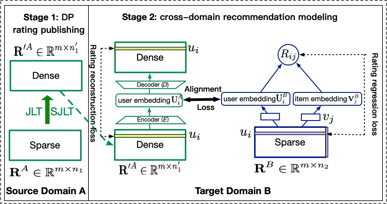
PriCDR consists of two stages, i.e., rating publishing and cross-domain recommendation modeling, as is shown in Figure 1. First, as described in Section 1, rating publishing mainly has three goals, i.e., G1: privacy-preserving, G2: restricted isometry property, and G3: sparse-aware. To achieve these goals, we propose two differential private rating matrix publishing algorithms, including JLT and SJLT. The former one achieves privacy-preserving and restricted isometry property while the later one further achieves sparse-aware, which will be further demonstrated both in theoretically in Sec. 5 and experimentally in Sec. 6. Second, to handle the heterogeneity between the published rating matrix of the source domain and the original rating matrix of the target domain, we propose a new cross-domain recommendation model (i.e., HeteroCDR). HeteroCDR has three parts, a rating reconstruction module for the published source domain, a rating regression module for the target domain, and a user embedding alignment module between the user embeddings of the source domain and target domain.
With our proposed two stages, PriCDR can not only protect rating privacy, but also take advantage of the characteristics of both domains. Thus, PriCDR can achieve comparable even better performance than most existing plaintext CDR models, as will be reported in Sec. 6. We will present these two stages in details.
4.3. Differential Private Rating Publishing
We first present the rating publish stage of PriCDR. We protect the source domain data by publishing the source domain rating matrix to the target domain utilizing differential privacy. To protect the individual user-item rating privacy, we want the rating publishing stage to satisfy differential privacy. For this purpose, we propose to publish the rating matrix in the source domain differential privately via JLT or SJLT, as is shown in Algorithm 1. The whole process of the rating publish stage can be divided into two procedures, i.e., perturb the singular values of the normalized rating matrix (lines 1-1) and transform the perturbed rating matrix by JLT or SJLT (lines 1-1). We now describe these procedures in details.
Explanation of hyper-parameters. First of all, we introduce the hyper-parameters used Algorithm 1. and are privacy-related hyper-parameters. We tune for different privacy budget and fix , where is number of input data. and are utility-related hyper-parameters to determine the subspace dimension after applying JLT or SJLT. The larger and , the smaller , the smaller probability we get for the concentration results in Theorem 5.4.
Perturb the singular values of the normalized rating matrix. Before applying random transforms on rating matrix, we apply singular value perturbation, which consists of four steps. The first step is to subtract the mean from rating matrix (line 1). The second step is to compute the compressed dimension and singular value perturbation (line 3). The third step is to compute the singular value decomposition of matrix and get the singular values as the non-zero elements of the diagonal matrix (line 4). The fourth step is to modify the singular values of by , where (line 5). By exerting proper singular value perturbation on the randomized rating matrix, we get a perturbed rating matrix with the same singular vectors but a different spectrum from the original rating matrix. In recommender systems, it is common to use the singular vectors corresponding to top singular values. Thus, we preserve the privacy by perturbing the singular values while maintaining utility by keeping singular vectors unchanged, which achieves G1: privacy-preserving.
Transform the perturbed rating matrix by JLT or SJLT. After the first procedure, one can transform the perturbed rating matrix randomly via JLT (line 7 and line 14) or SJLT (line 9-12 and line 14). By applying random transform, we exert a proper randomness on rating matrix where the magnitude is determined by perturbation parameter in the previous procedure. By the expectation approximation result (Proposition 5.3) and concentration result of Gaussian or sub-Gaussian random matrix ( Proposition C.1), we conclude that JLT and SJLT achieve G2: restricted isometry property ( see Theorem 5.4). The main difference between JLT and SJLT is how to generate the random matrix . The random matrix of JLT is generated by Gaussian ensemble, while that of SJLT is generated by sub-Gaussian ensemble and random Hadamard matrix, as described in Definition 3.7. By singular value perturbation and random transform with JLT or SJLT, we get a differentially privately published rating matrix . Compared with JLT, (1) SJLT can reduce the computation complexity of matrix multiplication by utilizing random Hardmard transform with computation complexity of while JLT costs (line 14). (2) the random hardmard transform in SJLT serves as a precondition when input is sparse (verified by Lemma 5.5), and thus SJLT achieves G3: sparse-awareness.
4.4. CDR Modeling
We then present the cross-domain modeling stage of PriCDR. The cross-domain modeling stage is done by the target domain by using the published rating matrix of the source domain and the original rating matrix of the target domain.
We propose a novel cross-domain recommendation model, i.e., HeteroCDR, to solve the heterogeneity between the published rating matrix of the source domain and the original rating matrix of the target domain. HeteroCDR has three parts: (1) a rating reconstruction module for the differential privately published source domain; (2) a rating regression module for the target domain; and (3) a user embedding alignment module between the user embeddings of the source domain and target domain. We will describe these three modules separately in detail.
Rating reconstruction of the source domain. Let be the private rating matrix of the source domain, be the published rating matrix of the source domain, and . Considering that is a dense matrix with each row denoting the perturbed behaviors of each user, we use auto-encoder to learn user embedding. Specifically, we can first obtain the user embedding by the encoder, i.e., , where is the dimension of user embedding. The autoencoder can then reconstruct the perturbed ratings of each user by . After it, the reconstruction loss is given by:
| (5) |
where is the mean square loss. With the rating reconstruction module, the encoder and decoder can model the perturbed user-item rating interactions in the source domain.
Rating regression of the target domain. The rating regression module in the target domain is similar as the existing deep neural network based recommendation models, e.g., Deep Matrix Factorization (DMF) (Xue et al., 2017) and Neural Matrix Factorization (NeuMF) (He et al., 2017). In this paper, we take DMF as an example. The key idea of DMF is to minimize the cross-entropy between the true ratings and the predicted ratings , where the predicted ratings is obtained by multiple fully-connected layers. Specifically, we first get the user and item latent embeddings and with denoting the embedding dimension, and then the predicted ratings are the cosine similarities between user and item latent embeddings, i.e., . Its loss function is given as:
| (6) |
where is the maximum rating in the target domain. With the rating regression module, we can model the user-item rating interactions in the target domain.
User embedding alignment between source and target domains. Although the rating reconstruction module and the rating regression module can model the perturbed ratings of the source domain and the original ratings of the target domain respectively, the knowledge learnt from the source domain cannot be transferred to the target domain yet. To facilitate the knowledge transfer between the source and target domains, we further propose a user embedding alignment module. The user embedding alignment module aims to match the user embedding learnt from the rating reconstruction module and the user embedding learnt from the rating regression module. Our motivation is that users tend to have similar preferences across different domains. For example, users who like romantic movies are likely to like romantic book as well. Formally, the user embedding alignment loss is given as:
| (7) |
Total loss. The loss of HeteroCDR is a combination of the three type of losses above. That is,
| (8) |
where is a hyper-parameter that controls the strength of the user embedding alignment module.
5. Analysis
5.1. Privacy Analysis
To analyze the privacy of Algorithm 1, we study how the output distribution changes for neighbouring rating matrices and how to achieve both user-level DP and rating matrix DP.
User-level differential privacy. We first present the user-level differential privacy, i.e., privacy loss for a single row in differential private published rating matrix. In Theorem 5.1, we show that both JLT and SJLT achieve user-level DP.
Theorem 5.1 (User-level Differential Privacy).
Proof.
We present its proof in Appendix B.1. ∎
Rating matrix differential privacy. Based on user-level privacy guarantees (Theorem 5.1) and the k-fold composition theorem (Theorem B.1 in Appendix), we present differential privacy with respect to rating value of Algorithm 1.
Theorem 5.2 (Rating Matrix Differential Privacy).
Algorithm 1 preserves differential privacy with respect to a single rating value changing in .
Proof.
We present its proof in Appendix B.2. ∎
By presenting privacy guarantees for user-level and rating matrix, we show our algorithm achieves G1: Privacy-preserving.
5.2. Utility Analysis
We analyze the utility of Algorithm 1 from a probabilistic perspective. First, we show that the expectation of the perturbed published rating matrix on the low-dimensional subspace approximates the input rating matrix on the high-dimensional original space, with a bias determined by privacy parameters (Theorem 5.3). Based on the expectation approximation, we show Algorithm 1 achieves Restricted isometry property, i.e., the output rating matrix concentrates around the mean approximation with a large probability determined by privacy parameters (Theorem 5.4).
Expectation approximation. We first present the approximation effect of the published rating matrix to original one, which is the foundation of restricted isometry property.
Proposition 5.3.
Let and be the input and output rating matrix of Algorithm 1, respectively. Then, the mean squared error of the input and output covariance matrices are
where is the dimension of the reduced item space, is the number of user, and are privacy parameters.
Proof.
We present its proof in Appendix C.1. ∎
Restricted isometry property. We then come to the main results— Algorithm 1 has Restricted isometry property.
Theorem 5.4 (Restricted Isometry Property).
Let and be the input and output rating matrix of Algorithm 1, respectively. Then
where is the dimension of reduced item space, is the number of user, and
Proof.
We present its proof in Appendix C.2. ∎
By the concentration results, we see that the larger subspace dimension , the larger probability approximated with a distance of , which verifies the conclusion.
Improvement of SJLT. Furthermore, we explain how SJLT improves JLT from the perspective of preconditioning. Applying SJLT on a vector , we have . Since and are unitary, preserves norm, i.e., .
Lemma 5.5 (Randomized Hardmard transform (Ailon and Chazelle, 2009)).
Let and be defined in Definition 3.7. For any set of vectors in , with probability at least ,
Proof.
We present its proof in Appendix C.3. ∎
By Lemma 5.5, we observe that the preconditioner reduces the norm of . With the same -norm and reduced norm, the energy of vector is spread out. That is, the preconditioner smoothes out the sparse vector and improves the utility of sparse sub-Gaussian transform . To this end, our algorithm achieves G2 (restricted isometry property) and G3 (sparse-aware).
6. Experiments and Analysis
In this section, we conduct experiments on two real-world datasets to answer the following research questions. RQ1: How can our model outperform the state-of-the-art recommendation model that is trained using the data of the target domain only? RQ2: What is the performance of our model compared with the state-of-the-art CDR models that are trained using both the plaintext source and target datasets? RQ3: Is our proposed CDR model (HeteroCDR) effective for the heterogeneous user-item rating data in the source and target domains? RQ4: How do the parameters of JLT and SJLT (mainly , , and ) in stage 1 affect our model performance? RQ5: Will different data sparsity in the source domain affect the performance of JLT and SJLT?
6.1. Experimental Setup
Datasets. We choose two real-world datasets, i.e., Amazon and Douban. The Amazon dataset (Ni et al., 2019; Zhao et al., 2020) has three domains, i.e., Movies and TV (Movie), Books (Book), and CD Vinyl (Music). The Douban dataset (Zhu et al., 2019, 2021b) also has three domains, i.e., Book, Music, and Movie. Since the user-item interaction ratings in both datasets range from 0 to 5, we binarize them by taking the ratings that are higher or equal to 3 as positive and others as negative, following (Hu et al., 2018). We also filter the users and items with less than 5 interactions. For simplification, we only choose the user-item interactions of the common users across domains. The detailed statistics of these datasets after pre-process are shown in Appendix D.
Comparison methods. To validate the performance of our proposed model, we compare PriCDR and its variants (PriCDR-SYM, PriCDR-J, and PriCDR-S) with both the famous single domain recommendation methods (BPR, NeuMF, and DMF) and the state-of-the-art CDR methods (CoNet, DDTCDR, DARec, and ETL). BPR (Rendle et al., 2012) is a representative pairwise learning-based factorization model, focusing on minimizing the ranking loss between predicted ratings and observed ratings. NeuMF (He et al., 2017) is a representative neural network based model, replacing the conventional inner product with a neural architecture to improve recommendation accuracy. DMF (Xue et al., 2017) is the state-of-the-art deep neural network based recommendation model, employing a deep architecture to learn the low-dimensional factors of users and items. CoNet (Hu et al., 2018) enables dual knowledge transfer across domains by introducing cross connections unit from one base network to the other and vice versa. DDTCDR (Li and Tuzhilin, 2020) introduces a deep dual transfer network that transfers knowledge with orthogonal transformation across domains. DARec (Yuan et al., 2019) transfers knowledge between domains with shared users, learning shared user representations across different domains via domain adaptation technique. ETL (Chen et al., 2020b) is a recent state-of-the-art CDR model that adopts equivalent transformation module to capture both the overlapped and the non-overlapped domain-specific properties. PriCDR-SYM is a comparative model for ablation study which replaces HeteroCDR with a symmetrical CDR framework, using auto-encoder to model both the published source rating matrix and the target rating matrix. PriCDR-SYM uses JLT based differential private rating matrix publishing mechanism. PriCDR-J is our proposed PriCDR with JLT based differential private rating matrix publishing mechanism in the first stage. PriCDR-S is our proposed PriCDR with Sparse-aware JLT based differential private rating matrix publishing mechanism.
Evaluation method. To evaluate the recommendation performance, We use the leave-one-out method which is widely used in literature (He et al., 2017). That is, we randomly reserve two items for each user, one as the validation item and the other as the test item. Then, following (He et al., 2017; Hu et al., 2018), we randomly sample 99 items that are not interacted by the user as the negative items. We choose three evaluation metrics, i.e., Hit Ratio (HR), Normalized Discounted Cumulative Gain (NDCG), and Mean Reciprocal Rank (MRR), where we set the cut-off of the ranked list as 5 and 10.
Parameter settings. For both source domain and target domain, we use two-layer MLP with hidden size of 500 and 200 as the network architecture and ReLU as the activation function. For a fair comparison, we choose Adam (Kingma and Ba, 2014) as the optimizer, and tune both the parameters of PriCDR and the baseline models to their best values. For differential private related parameters, we vary in and subspace dimension for the differential privately published rating matrix in . For SJLT, we vary the sparsity coefficient of the reduced matrix in . For CDR modeling, we set batch size to 128 for both the source and target domains. The dimension of the latent embedding is set to . Meanwhile we set the hyper-parameter for user embedding alignment, since it achieves the best performance. For all the experiments, we perform five random experiments and report the average results.
6.2. Model Comparison (RQ1 and RQ2)
We report the comparison results on Douban and Amazon datasets in Table 1. From the results, we can find that: (1) All the cross domain recommendations models (e.g., DARec) perform better than single domain recommendation (e.g., NeuMF) models, indicating that cross domain recommendations can integrate more useful information to enhance the model performance, which always conform to our common sense. (2) Our proposed PriCDR-J and PriCDR-S outperform all the single-domain and cross-domain baseline models in all tasks, which means the two-stage design of privacy-preserving CDR works well in predicting users’ preference in target domain while preserving the data privacy of the source domain at the same time. (3) By comparing the performance between PriCDR-J and PriCDR-S, we can conclude that Sparse-aware Johnson-Lindenstrauss Transform can effectively alleviate the data sparsity in the source domain, and thus significantly boosts the recommendation performance of PriCDR .
| HR@5 | NDCG@5 | MRR@5 | HR@10 | NDCG@10 | MRR@10 | HR@5 | NDCG@5 | MRR@5 | HR@10 | NDCG@10 | MRR@10 | |
| (Amazon) MusicBook | (Amazon) MovieMusic | |||||||||||
| BPR | 0.2633 | 0.2090 | 0.1827 | 0.3824 | 0.2580 | 0.2442 | 0.2448 | 0.1569 | 0.1734 | 0.3852 | 0.2035 | 0.1983 |
| NeuMF | 0.2760 | 0.2271 | 0.2086 | 0.4015 | 0.2577 | 0.2608 | 0.2937 | 0.1971 | 0.1988 | 0.4328 | 0.2401 | 0.2200 |
| DMF | 0.3075 | 0.2543 | 0.2367 | 0.4312 | 0.2713 | 0.2864 | 0.3316 | 0.2146 | 0.2266 | 0.4671 | 0.2715 | 0.2448 |
| CoNet | 0.3743 | 0.3157 | 0.3063 | 0.4831 | 0.3352 | 0.3245 | 0.3995 | 0.2857 | 0.2731 | 0.5328 | 0.3340 | 0.2973 |
| DDTCDR | 0.4067 | 0.3403 | 0.3241 | 0.5054 | 0.3690 | 0.3318 | 0.4311 | 0.3368 | 0.2974 | 0.5499 | 0.3736 | 0.3126 |
| DARec | 0.4741 | 0.3758 | 0.3420 | 0.5702 | 0.4098 | 0.3499 | 0.4916 | 0.3825 | 0.3402 | 0.6192 | 0.4220 | 0.3567 |
| ETL | 0.4769 | 0.3801 | 0.3462 | 0.5877 | 0.4153 | 0.3607 | 0.5308 | 0.4126 | 0.3714 | 0.6517 | 0.4511 | 0.3873 |
| PriCDR-SYM | 0.4360 | 0.3467 | 0.3172 | 0.5487 | 0.3828 | 0.3321 | 0.4933 | 0.3815 | 0.3445 | 0.6103 | 0.4192 | 0.3600 |
| PriCDR-J | 0.4898 | 0.3984 | 0.3648 | 0.5853 | 0.4292 | 0.3744 | 0.5399 | 0.4344 | 0.3992 | 0.6519 | 0.4706 | 0.4141 |
| PriCDR-S | 0.5203 | 0.4264 | 0.3964 | 0.6181 | 0.4580 | 0.4092 | 0.5733 | 0.4608 | 0.4220 | 0.6853 | 0.4970 | 0.4392 |
| (Amazon) MovieBook | (Douban) BookMusic | |||||||||||
| BPR | 0.2798 | 0.1665 | 0.2210 | 0.3716 | 0.2109 | 0.2392 | 0.1375 | 0.0822 | 0.0699 | 0.2889 | 0.1058 | 0.0950 |
| NeuMF | 0.3042 | 0.1989 | 0.2341 | 0.3999 | 0.2438 | 0.2403 | 0.1336 | 0.0913 | 0.0728 | 0.3042 | 0.1187 | 0.1093 |
| DMF | 0.3253 | 0.2281 | 0.2570 | 0.4238 | 0.2510 | 0.2439 | 0.1547 | 0.1003 | 0.0824 | 0.3315 | 0.1367 | 0.1100 |
| CoNet | 0.3744 | 0.2659 | 0.2978 | 0.4905 | 0.3050 | 0.3098 | 0.2044 | 0.1321 | 0.0996 | 0.3787 | 0.1633 | 0.1340 |
| DDTCDR | 0.4322 | 0.3490 | 0.3132 | 0.5288 | 0.3827 | 0.3355 | 0.2312 | 0.1425 | 0.1037 | 0.3934 | 0.1846 | 0.1506 |
| DARec | 0.4904 | 0.3824 | 0.3388 | 0.6034 | 0.4224 | 0.3552 | 0.2703 | 0.1878 | 0.1479 | 0.4285 | 0.2269 | 0.1711 |
| ETL | 0.5124 | 0.4119 | 0.3757 | 0.6339 | 0.4514 | 0.3915 | 0.3241 | 0.2161 | 0.1832 | 0.4545 | 0.2545 | 0.1987 |
| PriCDR-SYM | 0.4614 | 0.3665 | 0.3346 | 0.5801 | 0.4031 | 0.3496 | 0.3225 | 0.2113 | 0.1848 | 0.4535 | 0.2517 | 0.2002 |
| PriCDR-J | 0.5320 | 0.4324 | 0.3992 | 0.6423 | 0.4673 | 0.4135 | 0.3290 | 0.2208 | 0.1854 | 0.4675 | 0.2643 | 0.2034 |
| PriCDR-S | 0.5516 | 0.4483 | 0.4136 | 0.6585 | 0.4843 | 0.4285 | 0.3701 | 0.2582 | 0.2212 | 0.5097 | 0.3032 | 0.2397 |
| (Douban) MovieBook | (Douban) MovieMusic | |||||||||||
| BPR | 0.1827 | 0.1132 | 0.1091 | 0.3436 | 0.1590 | 0.1375 | 0.1572 | 0.1079 | 0.0959 | 0.3387 | 0.1635 | 0.1134 |
| NeuMF | 0.1989 | 0.1279 | 0.1124 | 0.3640 | 0.1748 | 0.1453 | 0.1641 | 0.0932 | 0.0947 | 0.3462 | 0.1577 | 0.1204 |
| DMF | 0.2376 | 0.1438 | 0.1321 | 0.3952 | 0.1940 | 0.1511 | 0.1889 | 0.1104 | 0.1082 | 0.3754 | 0.1823 | 0.1409 |
| CoNet | 0.2736 | 0.1724 | 0.1533 | 0.4407 | 0.2330 | 0.1996 | 0.2284 | 0.1358 | 0.1305 | 0.4193 | 0.2179 | 0.1748 |
| DDTCDR | 0.2984 | 0.1803 | 0.1776 | 0.4699 | 0.2487 | 0.2174 | 0.2457 | 0.1639 | 0.1522 | 0.4298 | 0.2375 | 0.1846 |
| DARec | 0.3331 | 0.2285 | 0.2109 | 0.4970 | 0.2789 | 0.2310 | 0.2990 | 0.2017 | 0.1835 | 0.4576 | 0.2608 | 0.2081 |
| ETL | 0.3850 | 0.2705 | 0.2348 | 0.5247 | 0.3157 | 0.2572 | 0.3383 | 0.2357 | 0.2008 | 0.4739 | 0.2862 | 0.2286 |
| PriCDR-SYM | 0.3742 | 0.2642 | 0.2310 | 0.5159 | 0.3094 | 0.2490 | 0.3194 | 0.2242 | 0.1930 | 0.4720 | 0.2737 | 0.2122 |
| PriCDR-J | 0.3926 | 0.2788 | 0.2421 | 0.5349 | 0.3248 | 0.2603 | 0.3450 | 0.2496 | 0.2197 | 0.4872 | 0.2922 | 0.2373 |
| PriCDR-S | 0.4301 | 0.3090 | 0.2702 | 0.5686 | 0.3503 | 0.2872 | 0.3801 | 0.2736 | 0.2440 | 0.5109 | 0.3158 | 0.2609 |
6.3. In-depth Model Analysis
Ablation study (RQ3). To study whether our model is effective for the heterogeneous user-item rating data, we compare PriCDR-J and PriCDR-S with PriCDR-SYM. The results from Table 1 show that both PriCDR-Jand PriCDR-S outperform PriCDR-SYM in all tasks, indicating that the heterogeneous CDR model we proposed in stage two makes it easier to handle the heterogeneity of rating data produced by stage one, and thus achieves a superior performance.
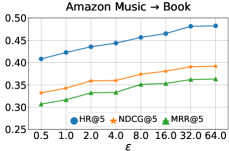
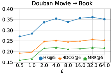
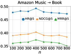
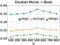
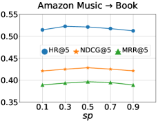
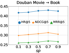
Parameter analysis (RQ4). We now study the effects of hyper-parameters on model performance. The most important parameters in PriCDR-J are the privacy parameter and subspace dimension . The key parameter in PriCDR-S is , which denotes the sparsity degree of the sparse Johnson-Lindenstrauss matrix. We report the results in Fig. 2-Fig. 4, where we use (Amazon) Music Book and (Douban) Movie Book datasets. Fig. 2 shows the effect of . With user-level differential privacy, the published rating matrix changes with subspace dimension . For details, please refer to Appendix B.2. We can find that the performance gradually improves when increases and finally keeps a stable level after reaches 32.0 in (Amazon) Music Book. And for the dataset (Douban) Movie Book, the turning point is when . We also vary and report the results in Fig. 3. The bell-shaped curve indicates that the accuracy will first gradually increase with and then slightly decrease, and PriCDR-J achieves the best performance when in (Amazon) Music Book and when in (Douban) Movie Book. Fig. 4 shows the effect of . The results show that when is small (e.g., 0.1), SJLT fails to grasp enough knowledge from the rating matrix in source domain. When is large (e.g., 0.9), SJLT gets redundant information from source domain rating matrix. A medium , e.g., 0.5 on (Amazon) Music Book and 0.7on (Douban) Movie Book, enables SJLT to grasp enough knowledge from the source domain rating matrix while exert an implicit regularization on optimization, and thus can achieve the best performance.
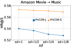
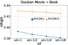
Effect of source domain sparsity (RQ5). To study the effect of source domain sparsity on the performance of JLT and SJLT, we change the sparsity of the source domain by sampling from the original dataset, such that the sparsity degree could be adjusted to . Here, denotes the original dataset without sampling. We report the results in Fig. 5, where we use (Amazon) Movie Music and (Douban) Movie Book datasets. From the results, we can conclude that: (1) The decrease of brings the decrease of the performance for both JLT and SJLT. (2) SJLT shows greater stability than JLT when the source domain becomes more sparse, which is owning to its sparse-aware ability, as we have analyzed in Sec. 5.2.
7. Conclusion
In this paper, we aim to solve the privacy issue in existing Cross Domain Recommendation (CDR) models. For this, we propose a novel two stage based privacy-preserving CDR framework, namely PriCDR. In stage one, the source domain privately publishes its user-item ratings to the target domain, and we propose two methods, i.e., Johnson-Lindenstrauss Transform (JLT) based and Sparse-aware JLT (SJLT) based, for it. We theoretically analyze the privacy and utility of our proposed differential privacy based rating publishing methods. In stage two, the target domain builds a CDR model based on its raw data and the published data of the source domain, and we propose a novel heterogeneous CDR model (HeteroCDR) for it. We empirically study the effectiveness of our proposed PriCDR and HeteroCDR on two benchmark datasets and the comprehensive experimental results show their effectiveness.
Acknowledgements.
This work was supported in part by the National Key R&D Program of China (No.2018YFB1403001) and the National Natural Science Foundation of China (No. 62172362 and No. 72192823).References
- (1)
- Ailon and Chazelle (2009) Nir Ailon and Bernard Chazelle. 2009. The fast Johnson–Lindenstrauss transform and approximate nearest neighbors. SIAM Journal on computing 39, 1 (2009), 302–322.
- Bhatia (2007) Rajendra Bhatia. 2007. Perturbation bounds for matrix eigenvalues. SIAM.
- Blocki et al. (2012) Jeremiah Blocki, Avrim Blum, Anupam Datta, and Or Sheffet. 2012. The johnson-lindenstrauss transform itself preserves differential privacy. In 2012 IEEE 53rd Annual Symposium on Foundations of Computer Science. IEEE, 410–419.
- Candes and Tao (2005) Emmanuel J Candes and Terence Tao. 2005. Decoding by linear programming. IEEE transactions on information theory 51, 12 (2005), 4203–4215.
- Chen et al. (2020a) Chaochao Chen, Liang Li, Bingzhe Wu, Cheng Hong, Li Wang, and Jun Zhou. 2020a. Secure Social Recommendation Based on Secret Sharing. In ECAI. 506–512.
- Chen et al. (2018) Chaochao Chen, Ziqi Liu, Peilin Zhao, Jun Zhou, and Xiaolong Li. 2018. Privacy Preserving Point-of-Interest Recommendation Using Decentralized Matrix Factorization. In AAAI. AAAI Press, 257–264.
- Chen et al. (2020b) Xu Chen, Ya Zhang, Ivor Tsang, Yuangang Pan, and Jingchao Su. 2020b. Towards Equivalent Transformation of User Preferences in Cross Domain Recommendation. arXiv preprint arXiv:2009.06884 (2020).
- Cui et al. (2021) Jinming Cui, Chaochao Chen, Lingjuan Lyu, Carl Yang, and Wang Li. 2021. Exploiting Data Sparsity in Secure Cross-Platform Social Recommendation. Advances in Neural Information Processing Systems (2021).
- Dasgupta and Gupta (2003) Sanjoy Dasgupta and Anupam Gupta. 2003. An elementary proof of a theorem of Johnson and Lindenstrauss. Random Structures & Algorithms 22, 1 (2003), 60–65.
- Dwork (2007) Cynthia Dwork. 2007. An ad omnia approach to defining and achieving private data analysis. In International Workshop on Privacy, Security, and Trust in KDD. Springer, 1–13.
- Dwork (2011) Cynthia Dwork. 2011. A firm foundation for private data analysis. Commun. ACM 54, 1 (2011), 86–95.
- Dwork et al. (2014) Cynthia Dwork, Aaron Roth, et al. 2014. The algorithmic foundations of differential privacy. Foundations and Trends in Theoretical Computer Science 9, 3-4 (2014), 211–407.
- Dwork et al. (2010) Cynthia Dwork, Guy N Rothblum, and Salil Vadhan. 2010. Boosting and differential privacy. In 2010 IEEE 51st Annual Symposium on Foundations of Computer Science. IEEE, 51–60.
- Gao et al. (2019a) Chen Gao, Xiangning Chen, Fuli Feng, Kai Zhao, Xiangnan He, Yong Li, and Depeng Jin. 2019a. Cross-domain recommendation without sharing user-relevant data. In The world wide web conference. 491–502.
- Gao et al. (2019b) Chen Gao, Chao Huang, Yue Yu, Huandong Wang, Yong Li, and Depeng Jin. 2019b. Privacy-preserving cross-domain location recommendation. Proceedings of the ACM on Interactive, Mobile, Wearable and Ubiquitous Technologies 3, 1 (2019), 1–21.
- He et al. (2017) Xiangnan He, Lizi Liao, Hanwang Zhang, Liqiang Nie, Xia Hu, and Tat-Seng Chua. 2017. Neural collaborative filtering. In Proceedings of the 26th international conference on world wide web. 173–182.
- Hu et al. (2018) Guangneng Hu, Yu Zhang, and Qiang Yang. 2018. Conet: Collaborative cross networks for cross-domain recommendation. In Proceedings of the 27th ACM international conference on information and knowledge management. 667–676.
- Hua et al. (2015) Jingyu Hua, Chang Xia, and Sheng Zhong. 2015. Differentially Private Matrix Factorization. In IJCAI. 1763–1770.
- Jiang et al. (2016) Wuxuan Jiang, Cong Xie, and Zhihua Zhang. 2016. Wishart Mechanism for Differentially Private Principal Components Analysis. In Proceedings of the Thirtieth AAAI Conference on Artificial Intelligence, February 12-17, 2016, Phoenix, Arizona, USA, Dale Schuurmans and Michael P. Wellman (Eds.). AAAI Press, 1730–1736.
- Kingma and Ba (2014) Diederik P Kingma and Jimmy Ba. 2014. Adam: A method for stochastic optimization. arXiv preprint arXiv:1412.6980 (2014).
- Li et al. (2021) Pan Li, Zhichao Jiang, Maofei Que, Yao Hu, and Alexander Tuzhilin. 2021. Dual Attentive Sequential Learning for Cross-Domain Click-Through Rate Prediction. In KDD ’21: The 27th ACM SIGKDD Conference on Knowledge Discovery and Data Mining, Virtual Event, Singapore, August 14-18, 2021, Feida Zhu, Beng Chin Ooi, and Chunyan Miao (Eds.). ACM, 3172–3180. https://doi.org/10.1145/3447548.3467140
- Li and Tuzhilin (2020) Pan Li and Alexander Tuzhilin. 2020. Ddtcdr: Deep dual transfer cross domain recommendation. In Proceedings of the 13th International Conference on Web Search and Data Mining. 331–339.
- Liu et al. (2021) Shuchang Liu, Shuyuan Xu, Wenhui Yu, Zuohui Fu, Yongfeng Zhang, and Amelie Marian. 2021. FedCT: Federated Collaborative Transfer for Recommendation. In Proceedings of the 44th International ACM SIGIR Conference on Research and Development in Information Retrieval. 716–725.
- Liu et al. (2015) Ziqi Liu, Yu-Xiang Wang, and Alexander J. Smola. 2015. Fast Differentially Private Matrix Factorization. In Proceedings of the 9th ACM Conference on Recommender Systems, RecSys 2015, Vienna, Austria, September 16-20, 2015, Hannes Werthner, Markus Zanker, Jennifer Golbeck, and Giovanni Semeraro (Eds.). ACM, 171–178. https://doi.org/10.1145/2792838.2800191
- McSherry and Mironov (2009) Frank McSherry and Ilya Mironov. 2009. Differentially private recommender systems: Building privacy into the netflix prize contenders. In Proceedings of the 15th ACM SIGKDD international conference on Knowledge discovery and data mining. 627–636.
- Ni et al. (2019) Jianmo Ni, Jiacheng Li, and Julian McAuley. 2019. Justifying Recommendations using Distantly-Labeled Reviews and Fine-Grained Aspects. In EMNLP-IJCNLP. 188–197. https://doi.org/10.18653/v1/D19-1018
- Nikolaenko et al. (2013) Valeria Nikolaenko, Stratis Ioannidis, Udi Weinsberg, Marc Joye, Nina Taft, and Dan Boneh. 2013. Privacy-preserving matrix factorization. In Proceedings of the 2013 ACM SIGSAC conference on Computer & communications security. 801–812.
- Ogunseyi et al. (2021) Taiwo Blessing Ogunseyi, Cossi Blaise Avoussoukpo, and Yiqiang Jiang. 2021. Privacy-Preserving Matrix Factorization for Cross-Domain Recommendation. IEEE Access (2021).
- Rendle et al. (2012) Steffen Rendle, Christoph Freudenthaler, Zeno Gantner, and Lars Schmidt-Thieme. 2012. BPR: Bayesian personalized ranking from implicit feedback. arXiv preprint arXiv:1205.2618 (2012).
- Wikipedia contributors (2021) Wikipedia contributors. 2021. Chernoff bound — Wikipedia, The Free Encyclopedia. https://en.wikipedia.org/w/index.php?title=Chernoff_bound&oldid=1050419718 [Online; accessed 18-October-2021].
- Xue et al. (2017) Hong-Jian Xue, Xinyu Dai, Jianbing Zhang, Shujian Huang, and Jiajun Chen. 2017. Deep Matrix Factorization Models for Recommender Systems.. In IJCAI, Vol. 17. Melbourne, Australia, 3203–3209.
- Yuan et al. (2019) Feng Yuan, Lina Yao, and Boualem Benatallah. 2019. DARec: Deep Domain Adaptation for Cross-Domain Recommendation via Transferring Rating Patterns. In Proceedings of the Twenty-Eighth International Joint Conference on Artificial Intelligence, IJCAI 2019, Macao, China, August 10-16, 2019, Sarit Kraus (Ed.). ijcai.org, 4227–4233. https://doi.org/10.24963/ijcai.2019/587
- Zhao et al. (2020) Cheng Zhao, Chenliang Li, Rong Xiao, Hongbo Deng, and Aixin Sun. 2020. CATN: Cross-Domain Recommendation for Cold-Start Users via Aspect Transfer Network. 229–238. https://doi.org/10.1145/3397271.3401169
- Zhu et al. (2019) Feng Zhu, Chaochao Chen, Yan Wang, Guanfeng Liu, and Xiaolin Zheng. 2019. Dtcdr: A framework for dual-target cross-domain recommendation. In CIKM. 1533–1542.
- Zhu et al. (2021a) Feng Zhu, Yan Wang, Chaochao Chen, Jun Zhou, Longfei Li, and Guanfeng Liu. 2021a. Cross-Domain Recommendation: Challenges, Progress, and Prospects. In IJCAI. 4721–4728.
- Zhu et al. (2021b) Feng Zhu, Yan Wang, Jun Zhou, Chaochao Chen, Longfei Li, and Guanfeng Liu. 2021b. A unified framework for cross-domain and cross-system recommendations. IEEE Transactions on Knowledge and Data Engineering (2021).
Appendix A Notations
We summarize the main notations used in this paper in Table 2.
| Notation | Meaning |
|---|---|
| privacy hyper-parameters in DP | |
| utility hyper-parameters in DP | |
| matrix of all elements equal one | |
| identity matrix | |
| normalized Hadamard matrix | |
| randomized diagonal matrix | |
| Gaussian random matrix | |
| sub-Gaussian random matrix |
Appendix B Privacy Analysis
B.1. User-level Differential Privacy
Proof.
To achieve privacy-preserving property, we need to verify the user-level differential privacy as JLT described in Theorem 5.1. As defined in Definition 3.2, we suppose two neighbouring rating matrix and with a rank-1 gap, i.e., Suppose the SVD decomposition of and are and Due to the limited space, we present the proof for the scenario that both singular values of and are greater than the perturbation parameter . The general case is an extension of this proof combined with the results in (Blocki et al., 2012). To achieve the user-level differential privacy of JLT, we considere the difference between the two distributions as
where and is a random vector sampled from Then we have two stage results. Firstly,
| (9) |
Secondly,
By Lindskii’s theorem on rank-1 perturbation (Theorem 9.4 in (Bhatia, 2007)), we have , and thus Equation (9) naturally holds. For the second result, by the discussion in (Blocki et al., 2012), we have
To achieve DP on user-level, we solve the following inequality exactly
We have
Since , we have
Thus, by choosing we have Algorithm 1 with JLT satisfies user-level DP. Then we discuss the case of Algorithm 1 with SJLT. By the construction of SJLT in Definition 3.7, we have two good properties for Algorithm 1.
-
•
and are unitary, i.e.,
-
•
Rows in are sub-Gaussian,
where is constructed by concatenating i.i.d. sparse random Gaussian vectors which is generated by
In order to check the distribution between and , we compare the difference in Probability Density Function (PDF) of a single row in and , i.e., and , with denoting a sub-Gaussian vector. Then the privacy of Algorithm 1 with SJLT follows the same procedure as JLT.
∎
B.2. Rating Matrix Differential Privacy
By user-level differential privacy, we then compare the distribution difference on probability density function of a single row in output rating matrix and . To analyze the difference of two whole rating matrices and , we utilize the following composition theorem presented in Theorem B.1.
Composition Theorem. By user-level differential privacy, we then compare the distribution difference on probability density function of a single row in output rating matrix and . To analyze the difference of two whole rating matrices and , we utilize the following composition theorem presented in Theorem B.1.
Theorem B.1 (Composition Theorem (Dwork et al., 2010)).
For every , and the class of differential private mechanisms is differentially private under fold adaptive composition, for
| (10) |
where
Proof of rating matrix differential privacy. We simply describe the proof as follows.
Appendix C Utility Analysis
C.1. Expectation Approximation
Proof.
Let be the input rating matrix. The SVD decomposition of is
After the singular value perturbation, we have
Then the output rating matrix is
where is the random matrix generated by Definition 3.6 or 3.7.
Then we consider the expectation mean squared error of covariance matrices,
The last equality is confirmed by the property of Gaussian orthogonal ensemble, i.e.,
Thus
with .
∎
Before prove RIP (Theorem 5.4), we present the proposition used in proving Johnson-Lindenstrauss Lemma (Dasgupta and Gupta, 2003).
Proposition C.1.
Let and be either JLT or SJLT. Let , and Then
C.2. Restricted Isometry Property
Proof.
Let be the column vector of rating matrix for respectively. Each represents the user-item rating list for user . Let Then
By Proposition C.1, we have
Denote the event and By the fact and each row of are pairwise independent. We have
To conclude, we have
Similarly,
Thus
∎
C.3. Preconditioning Effect of Randomized Hardmard Transform
Proof.
Without loss of generality,we supoose . Denote For each , , where Then we can compute the moment generating function of ,
By the results of Chernoff tail bound (Wikipedia contributors, 2021), we have
Let , and sum over coordinates, we have the desired result. ∎
Appendix D Datasets Description
We conduct extensive experiments on two popularly used real-world datasets, i.e., Amazon and Douban, for evaluating our model on CDR tasks. First, the Amazon dataset has three domains, i.e., Movies and TV (Movie), Books (Book), and CDs and Vinyl (Music) with user-item ratings. Second, the Douban dataset has three domains, i.e., Book, Movie and Music. We show the detailed statistics of these datasets after pre-process in Table 3.
| Datasets | Users | Items | Ratings | Density | |
|---|---|---|---|---|---|
| Amazon | Music | 16,367 | 18,467 | 233,251 | 0.08% |
| Book | 23,988 | 291,325 | 0.07% | ||
| Amazon | Movie | 15,914 | 19,794 | 416,228 | 0.13% |
| Music | 20,058 | 280,398 | 0.08% | ||
| Amazon | Movie | 29,476 | 24,091 | 591,258 | 0.08% |
| Book | 41,884 | 579,131 | 0.05% | ||
| Douban | Book | 924 | 3,916 | 50,429 | 1.39% |
| Music | 4,228 | 50,157 | 1.28% | ||
| Douban | Movie | 1,574 | 9,471 | 744,983 | 4.99% |
| Book | 6,139 | 85,602 | 0.89% | ||
| Douban | Movie | 1,055 | 9,386 | 557,989 | 5.63% |
| Music | 4,981 | 60,626 | 1.15% | ||