Understanding Hyperdimensional Computing for Parallel Single-Pass Learning

Abstract

Hyperdimensional computing (HDC) is an emerging learning paradigm that computes with high dimensional binary vectors. There is an active line of research on HDC in the community of emerging hardware because of its energy efficiency and ultra-low latency—but HDC suffers from low model accuracy, with little theoretical understanding of what limits its performance. We propose a new theoretical analysis of the limits of HDC via a consideration of what similarity matrices can be “expressed” by binary vectors, and we show how the limits of HDC can be approached using random Fourier features (RFF). We extend our analysis to the more general class of vector symbolic architectures (VSA), which compute with high-dimensional vectors (hypervectors) that are not necessarily binary. We propose a new class of VSAs, finite group VSAs, which surpass the limits of HDC. Using representation theory, we characterize which similarity matrices can be “expressed” by finite group VSA hypervectors, and we show how these VSAs can be constructed. Experimental results show that our RFF method and group VSA can both outperform the state-of-the-art HDC model by up to 7.6% while maintaining hardware efficiency. This work aims to inspire a future interest on HDC in the ML community and connect to the hardware community.

1 Introduction

Hyperdimensional computing (HDC) is an emerging learning paradigm. Unlike conventional cognitive modeling that computes with real numbers, it computes with high dimensional binary vectors, referred to as binary hypervectors, the dimension of which is usually at least in the thousands. HDC is brain-inspired as high dimensional representations have two fundamental properties similar to human brains: they are (1) distributed and highly parallel; and (2) robust to noise and tolerant to component failure (Kanerva, 2009). On the other hand, the massive parallelism and simple arithmetic project HDC into the scope of energy-efficient and ultra-low-latency computing, especially with the rise of emerging hardware (Imani et al., 2021, 2020; Gupta et al., 2020; Salamat et al., 2019). As a result, HDC has recently attracted considerable attention from edge applications, e.g., robotics, DNA pattern matching, and health diagnosis, as well as data center applications such as recommendation systems (Mitrokhin et al., 2019; Neubert et al., 2019; Neubert and Schubert, 2021; Kim et al., 2020; Burrello et al., 2019; Guo et al., 2021).

The practical deployment of HDC is undermined by its low model accuracy compared to other alternatives, e.g., neural networks (NN). The state-of-the-art HDC model on MNIST has an accuracy of $89$% (Chuang et al., 2020). A two-layer NN, however, can easily achieve $95$% (Lecun et al., 1998).

There are two main approaches in the literature to improving HDC. One approach is to increase the hypervector dimension, staying within the classic HDC paradigm and just making the binary vectors longer (Neubert et al., 2019; Schlegel et al., 2021). An alternative is to increase the complexity of each element in a hypervector, e.g., to floating-point or complex numbers (unit circle in the complex plane) (Plate, 1995; Gallant and Okaywe, 2013; Gayler, 1998; Plate, 1994): this moves the system into the more general realm of vector symbolic architecture (VSA) (Schlegel et al., 2021), which uses high-dimensional vectors with elements that are not necessarily binary (unlike binary HDC). However, these remedies are not based on any theoretical analysis of the limits of HDC, and as a result there is a lack of more-than-empirical understanding of when and how they should be deployed.

In this work, we introduce a new notion of expressivity for any VSA using similarity matrices. Given a set of hypervectors $v_{1},\ldots,v_{n}$ in a VSA, each entry $\mathbf{M}_{ij}$ in the similarity matrix $\mathbf{M}$ is defined as the similarity between a pair of hypervectors $v_{i}$ and $v_{j}$; the similarity is typically measured by an inner product function. Informally, we propose that a VSA is more expressive when it can express (i.e. represent with some set of vectors) a wider class of similarity matrices. Importantly, which $\mathbf{M}$ a VSA can express is independent of the vector dimension $D$: this new notion distinguishes between longer-vector and more-complex-vector approaches.

We show that HDC, with binary hypervectors even in any dimension, cannot express as many similarity matrices that a VSA with more complex hypervectors can. Even worse, the current method of initializing the hypervectors in an HDC system further reduces the expressible set, which impedes the success of HDC. This notion of expressivity is closely related to learning ability. We exhibit a simple task where current HDC (of any $D$) is incapable of learning a Bayes optimal classifier, while any other VSA system that can express a particular similarity matrix $\mathbf{M}$ (which HDC cannot express) can learn it through the same procedure.

Based on our analysis, we investigate how we can improve HDC through the lens of similarity matrices. We first propose to improve the initialization of binary hypervectors by employing random Fourier features (RFFs) (Rahimi and Recht, 2007). This method is different from existing approaches that increase the dimension or complexity of hypervectors. We show that this better initialization via expressing a similarity matrix can already surpass state-of-the-art HDC accuracy on MNIST by $6.4$%. We then propose and formally define group VSA, an extended version of HDC where elements in hypervectors are more complex than binary but less than floating-point. Group VSA can further improve the RFF-initialized HDC by $1.2$% on MNIST.

Our contributions are as follows:

• We provide a theoretical analysis of the limitations of an HDC system with binary hypervectors.

• We approach the expressivity limit of HDC systems with random Fourier features and empirically evaluate the improvements on standard benchmarks.

• We propose group VSA, which generalizes HDC with more complex elements, expanding the set of expressible similarity matrices while maintaining efficiency.

• We evaluate the performance of group VSA on both conventional HDC tasks and image tasks, and study its efficiency implications by analyzing the circuit depths.

2 Related Work

The term HDC was first introduced by Kanerva (2009). It is also referred to as VSA in some literature (Schlegel et al., 2021), a line of work that does symbolic computing. Binary HDC can be traced back to Binary Spatter Code (BSC) (Kanerva, 1994; Kanerva et al., 1997).

Model capacity improvement. There are two main VSA formats other than binary HDC: using floating-point real vectors (Plate, 1995; Gallant and Okaywe, 2013; Gayler, 1998; Gosmann and Eliasmith, 2019) or complex vectors (Plate, 1994). Typically their model capacities are higher since their individual vector components are more complex. Another way of increasing the model capacity is increasing the vector length (Neubert et al., 2019; Schlegel et al., 2021; Chuang et al., 2020; Frady et al., 2018). However, it remains unknown when and how we should apply these methods, and whether they are sufficient to solve a task. Our approach is different as our proposed methods are based on the theoretical analysis of, and are designed to bypass, the limits of binary HDC.

Hardware implication. HDC inspires a novel hardware architecture that requires associative memory (Hopfield, 1982) where long vectors can be stored and addressed efficiently. It is therefore popularized recently in the emerging in-memory computing community (Imani et al., 2020; Gupta et al., 2020). In the meantime, the simplicity of HDC arithmetic and the massive parallelism make HDC suitable for tasks that require high energy efficiency and low latency. It has been demonstrated successful on commercial hardware as well (Imani et al., 2021; Salamat et al., 2019; Basaklar et al., 2021). In this work, we provide an analysis on the circuit depths of HDC and our proposed group VSA.

Theory. Understanding HDC from a theoretical perspective is currently limited. Thomas et al. (2020); Frady et al. (2018) presented some theoretical foundations of HDC, introducing the benefit of high-dimensional vectors, hypervector encoding, and the connection between HDC and kernel approximation. Our work instead presents the limits of HDC and how we can bypass it. Frady et al. (2021) propose to generalize VSA/HDC to function space. Our work is different since our proposed group VSA, a generalization of HDC, is still discrete and preserves the hardware efficiency.

3 Background on HDC

In this section we introduce basics of HDC: hypervectors, arithmetic, and the learning paradigm. We then present a classical approach of HDC on the popular MNIST database. A more comprehensive introduction is in Ge and Parhi (2020).

HD Representations. In HDC, we compute with binary hypervectors in a high-dimensional space referred to as hyperspace. Given a random hypervector $v$ in a $10,000$ dimensional space $\{-1,1\}^{10,000}$, it is well known from the “curse” of dimensionality that most vectors in this hyperspace are nearly orthogonal to $v$ (Kanerva, 2009). We call such hypervectors unrelated. The “curse” provides two intriguing properties for cognitive tasks: (1) independent random hypervectors will be unrelated and so can naturally represent objects that are semantically separate, e.g. letters of the alphabet; (2) two hypervectors $u$ and $v$ that have a high-enough inner-product similarity can be classified as being related (i.e. somehow dependent) with high probability. Classical HDC therefore represents data using binary hypervectors randomly drawn from a hyperspace. HDC computes with hypervectors using a fixed set of primitive operations: similarity, binding, bundling, and permutation.

Similarity. A similarity function $\mathcal{S}(u,v)$ measures how close two hypervectors $u,v\in\{-1,1\}^{D}$ are. It is typically defined as an inner product function (Frady et al., 2021) $\mathcal{S}(u,v)=\frac{1}{D}\sum_{i=1}^{D}u_{i}v_{i}$; this is an affine function of the hamming distance for binary hypervectors (Kanerva, 2009).

Binding $\bigotimes$. The binding operation combines two hypervectors $u,v$ into a new hypervector in the same space that represents them as a pair. For binary $\{-1,+1\}^{D}$, binding is equivalent to coordinate-wise multiplication, i.e. $(u\otimes v)\in\{-1,+1\}^{D}$ and $(u\otimes v)_{i}=u_{i}v_{i}$ for all $i\in\{1,\ldots,D\}$. Binding preserves similarity, in the sense that $\mathcal{S}(u\otimes w,v\otimes w)=\mathcal{S}(u,v)$ for any hypervectors $u$, $v$, and $w$; also, if $u$ is highly similar to $v$ and $x$ is highly similar to $y$, then $u\otimes x$ will be highly similar to $v\otimes y$ (although usually less than either constituent pair). Binding is implemented on hardware as an XOR.

Bundling $\bigoplus$. Bundling represents an unordered collection of hypervectors. The bundling operation takes in a set of hypervectors and yields a hypervector that is maximally similar to all of them: it acts as an aggregation of a set of hypervectors. Bundling $v_{1},\ldots,v_{m}\in\{-1,+1\}^{D}$ yields $\left(\bigoplus_{k=1}^{m}v_{k}\right)_{i}=\operatorname*{sgn}\left(\sum_{k=1}^{m}\left(v_{k}\right)_{i}\right)\text{ for all }i\in\{1,\ldots,D\}$. This takes a majority vote at each coordinate of the vector; ties are broken at random. HDC typically leverages bundling to learn a class representative.

Permutation $\prod$. The permutation operation is a shuffling of the elements in a hypervector. It can be represented as a multiplication of a permutation matrix $\Pi$. A random permutation on a hypervector yields another hypervector that is unrelated to it. Note that permutation is invertible, meaning that $\Pi^{-1}\Pi v_{i}=v_{i}$. It is thus useful for encoding order and position information. In hardware, permutation usually appears as shifting since its implementation is efficient.

3.1 MNIST as a Case Study

We outline how to use the classic HDC approach on the MNIST digit recognition task for illustration.

Encoding. First, 256 basis hypervectors $\{v_{0},v_{1},\dots,v_{255}\}$ are independently drawn at random from a hyperspace $\{-1,+1\}^{D}$: each hypervector $v_{i}$ represents a pixel intensity $i$. Second, we bind all 784 pixels in an MNIST image by their corresponding hypervectors. Since the binding operation is commutative by definition, but pixels in an image have meaningful relative positions, each pixel hypervector is shifted before joining the encoding to preserve that position information. If the input pixel intensities are $p_{0},p_{1},\ldots,p_{783}$, then its encoded hypervector $t$ is $v_{p_{0}}\otimes(\Pi v_{p_{1}})\otimes\cdots\otimes({\Pi}^{783}v_{p_{783}})$, where ${\Pi}^{j}$ denotes shifting a hypervector $j$ times.

Learning. Encoding yields a set of training hypervectors $\mathbb{T}=\{t_{1},t_{2},\dots,t_{60,000}\}$. To learn, we bundle all the hypervectors that are from the same digit. Concretely, a class centroid $s_{c}$ is computed by $s_{c}=\bigoplus_{i|y_{i}=c}t_{i}$. Each training image is used only once, making this process single-pass learning.

Inference. At the inference time, a given test image is encoded through the same procedure. The model outputs the class $c$ with the highest similarity $\mathcal{S}(t_{\text{test}},s_{c})$.

4 Similarity Matrices and the Limits of HDC

Traditionally the expressivity of HDC setups is identified with the dimension of the hypervectors $D$. This notion is unhelpful for probing the fundamental limitations of HDC, which do not depend on $D$. In this section, we define a new notion of expressivity, which reveals the limits of HDC.

Definition 1.

An HDC (or VSA) system can express a similarity matrix $\mathbf{M}\in\mathbb{R}^{n\times n}$ if for any $\varepsilon>0$, there exists a $D\in\mathbb{N}$ and $D$-dimensional hypervectors $v_{1},v_{2},\ldots,v_{n}$ in the HDC/VSA such that $|\mathbf{M}_{ij}-\mathcal{S}(v_{i},v_{j})|\leq\varepsilon$ where $\mathcal{S}$ denotes the similarity function of the HDC/VSA.

Informally, this means that the HDC/VSA can approximate $\mathbf{M}$ arbitrarily well. Limitations on $\mathbf{M}$ we can express correspond to limitations on the similarity relation we can represent on data: if we have some dataset and know how similar each pair of examples should be, whether or not we can represent the similarity accurately with an HDC embedding depends on whether HDC can express the corresponding $\mathbf{M}$. Surprisingly, there are some matrices that an HDC system can never express.

Lemma 4.1.

Binary HDC can not express the matrix $\mathbf{M}_{\textup{Lemma \ref{lem:sim_hdc_fail}}}=\frac{3}{2}I_{3}-\frac{1}{2}\mathbf{1}_{3\times 3}.$

Our notion of expressivity corresponds to learning ability, we give an example task for which whether a VSA/HDC approach can learn the Bayes-optimal classifier depends on whether it can express $\mathbf{M}_{\textup{Lemma \ref{lem:sim_hdc_fail}}}$. Consider a supervised learning task with input set $\mathcal{X}=\{0,1,2\}$, output label set $\mathcal{Y}=\mathcal{X}$, and source distribution $\mathcal{P}(x,y)\!:=\!(1/9+2p)~{}\textit{if}~{}x=y~{}\textit{else}~{}(1/9-p)$ for some small positive number $p$. We say that a VSA can learn this task if there exists a $D$-dimensional encoding of $\mathcal{X}$ in that VSA such that, when the bundling method in Section 3.1 is used on a training set of size $N$ drawn from $\mathcal{P}$, the resulting classifier is the Bayes optimal classifier with arbitrarily high probability as $N$ increases.

Statement 4.1.

Binary HDC cannot learn this task. Any VSA (formalized later in Definition 2) that can express $\mathbf{M}_{\textup{Lemma \ref{lem:sim_hdc_fail}}}$ can learn this task.

Details on Statement 4.1 are in appendix. This learning task shows that only increasing the dimensionality of hypervectors cannot help learn the correct predictions if unable to express a certain matrix. This implies that our notion of expressivity captures HDC limitations in a way that relates to learning.

Limitations due to initialization. So far in this section we have described limitations that are inherent to using binary representations in a VSA. Classical HDC methods are often limited in an additional way: rather than considering arbitrary binary hypervectors, they use hypervectors that are sampled independently at random. In such a system, any hypervector used for an embedding (used to represent an entity) is constructed either by (1) independently sampling a binary hypervector where each entry has some probability $p$ of being $1$, or (2) permuting and/or binding some pre-existing hypervectors. Examples of this setup can be found in Burrello et al. (2019); Smith and Stanford (1990); Imani et al. (2019b). Surprisingly, we show that this approach further restricts the set of similarity matrices that can be expressed in expectation.

Lemma 4.2.

Let $u_{1},u_{2},\ldots,u_{K}$ be binary vectors sampled coordinate-wise independently at random, where each coordinate of $u_{i}$ has the same probability $p_{i}$ of being $1$. Let $v_{0}$, $v_{1}$, and $v_{2}$ be vectors that result from some composition of binding and permutation operations acting on $u_{1},\ldots,u_{K}$, and let $\mathbf{M}\in\mathbb{R}^{3\times 3}$ be their similarity matrix, such that $\mathbf{M}_{ij}=\mathcal{S}(v_{i},v_{j})$. Then

$$\textstyle\left\|\operatorname*{\mathbb{E}}[\mathbf{M}]-\left(\begin{smallmatrix}1&-\frac{1}{3}&-\frac{1}{3}\\ -\frac{1}{3}&1&-\frac{1}{3}\\ -\frac{1}{3}&-\frac{1}{3}&1\\ \end{smallmatrix}\right)\right\|_{F}\geq\frac{\sqrt{2}}{3},$$

but this target matrix can be expressed by binary HDC.

5 Encoding Hypervectors via RFF

Our analysis using similarity matrices provides a strong motivation for using more principled methods to construct hypervectors. We argue that, if there is some similarity matrix $\mathbf{M}$ we want to achieve, we should directly instantiate hypervectors to match it in expectation.

Algorithm 1 Construct correlated hypervectors

  input: similarity matrix $\mathbf{M}\in\mathbb{R}^{n\times n}$, dimension $d$

  let $\hat{\Sigma}=\sin(\frac{\pi}{2}\mathbf{M})$ {elementwise}

  let $U\Lambda U^{T}=\hat{\Sigma}$ {symmetric eigendecomposition}

  sample $X\in\mathbb{R}^{n\times d}$ iid unit Gaussians

  return $\operatorname*{sgn}(U\Lambda_{+}^{1/2}X)$ {elementwise}

A natural way to represent a desired similarity matrix $\mathbf{M}\in\mathbb{R}^{n\times n}$ is to project it onto the set of representable matrices of binary vectors, which would correspond to a distribution one could sample from. Unfortunately, this approach is intractable as it would require solving a linear programming problem of size exponential in $n$. Instead, to approach the expressivity limits of binary HDC, we propose the following approach, given in Algorithm 1. First, we sample $d$ independent multivariate Gaussians over $\mathbb{R}^{n}$; Our $n$ HDC vectors of length $d$ are then given by the signs of these Gaussians. The following lemma tells us how to make this produce a desired similarity matrix $\mathbf{M}$.

Lemma 5.1.

Suppose $X,Y$ are jointly Gaussian zero-mean unit-variance random variables, then $\operatorname*{\mathbb{E}}[\operatorname*{sgn}(X)\operatorname*{sgn}(Y)]=\frac{2}{\pi}\arcsin\left(\operatorname*{\mathbb{E}}[XY]\right).$

From this lemma, it immediately follows that if the elementwise $\sin$ of $\frac{\pi}{2}\mathbf{M}$ is positive semi-definite, then Algorithm 1 produces hypervectors that, in expectation, exactly achieve $\mathbf{M}$; otherwise, some approximation to $\mathbf{M}$ is produced. It also immediately follows that Algorithm 1 can achieve more similarity matrices than the classical procedure of Lemma 4.2: while that lemma shows that the similarity matrix $\frac{4}{3}I_{3}-\frac{1}{3}\mathbf{1}_{3\times 3}$ cannot be achieved in expectation by classical HDC initialization, Algorithm 1 can achieve it as $\sin(\frac{\pi}{2}\cdot\frac{-1}{3})=\frac{-1}{2}$ and $\frac{3}{2}I_{3}-\frac{1}{2}\mathbf{1}_{3\times 3}$ is positive semidefinite.

Algorithm 1 gives us more freedom to achieve a wider range of similarity matrices; however, it does not tell us which similarity matrix $\mathbf{M}$ to choose for a given task and whether $\sin(\frac{\pi}{2}\mathbf{M})$ is positive semi-definite or not. In this paper, we use the well-known RBF kernel (Vert et al., 2004) to choose the similarity matrix between entities, but any similarity matrix appropriate for a task is applicable.

6 Group VSA

So far we have shown how replacing existing initialization methods can approach the limits of binary HDC. However, as Lemma 4.1 shows, binary HDC itself has inherent limits. Other known VSAs, such as the unit cycle VSA (Plate, 1994)—in which the elements are complex numbers of absolute value $1$—can surpass these limits. However, this comes with the problem of a continuous space—requiring both approximation and significant hardware complexity overhead compared to binary HDC. In this section, we propose a new class of VSA, finite group VSA, which effectively “interpolates” between them so as to bypass the similarity-representation limits of binary HDC without the need for a continuous space.

We start by defining a VSA, and then propose to use group structures for the elements of hypervectors as a different approach to improve the expressivity of VSA. Binary HDC can be considered as a special case of our construction corresponding to the 2-element group.

Definition 2.

A group VSA is a tuple $(G,\mu,\otimes,\mathcal{S},\oplus)$, where $G$ is some measurable set of symbols, $\otimes:G\times G\rightarrow G$ is the binding operator, $\mathcal{S}:G\times G\rightarrow\mathbb{R}$ is a symmetric similarity operator, and $\oplus:G^{<\omega}\rightarrow G$ is the bundling operator (which maps a finite sequence of symbols to a symbol). A VSA must have the following properties:

• Binding. $(G,\otimes)$ is a group,​ i.e., binding is associative over $G$ and has inverse and identity elements.

• Similarity to self. $\mathcal{S}(x,x)=1$ for all $x\in G$.

• Similarity preserved by binding. $\mathcal{S}(g\otimes x,g\otimes y)=\mathcal{S}(x\otimes g,y\otimes g)=\mathcal{S}(x,y)$ for all $g,x,y\in G$.

• Similarity extensible to an inner product. There exists a finite-dimensional Hilbert space $V$ over $\mathbb{R}$ and an embedding $\psi:G\rightarrow V$ such that $\mathcal{S}(x,y)=\langle\psi(x),\psi(y)\rangle$ for all $x,y\in G$. Equivalently, $\sum_{i=1}^{n}\sum_{j=1}^{n}c_{i}c_{j}\mathcal{S}(x_{i},x_{j})\geq 0$ for any $x_{1},\ldots,x_{n}\in G$ and scalars $c_{1},\ldots,c_{n}\in\mathbb{R}$.

• Random vectors are dissimilar to any other vector. $\operatorname*{\mathbb{E}}_{g\sim\operatorname{Uniform}(G)}[\mathcal{S}(g,x)]=0$ for any $x\in G$.

• Bundling. Bundling of $x_{1},\ldots,x_{m}\in G$ returns $\bigoplus_{i=1}^{m}x_{i}=\arg\max_{g\in G}\;\sum_{i=1}^{m}\mathcal{S}(g,x_{i})$ or one of the maxima in case of a tie.

To compute using a VSA of dimension $D$, we use hypervectors in $G^{D}$, extend binding and bundling to act elementwise on these hypervectors, and extend similarity to compute the average similarity over the dimensions as $\mathcal{S}([x_{1},\ldots,x_{D}],[y_{1},\ldots,y_{D}])=\frac{1}{D}\sum_{i=1}^{D}\mathcal{S}(x_{i},y_{i})$. It is easy to see that binary HDC is equivalent to a VSA where $G=\{-1,1\}$, $\otimes$ is multiplication, and $\mathcal{S}(x,y)=xy$. Similarly, a unit-cycle VSA (i.e., FHRR) has $G=\{z\in\mathbb{C}\mid|z|=1\}$, $\otimes$ as complex multiplication, and $\mathcal{S}(x,y)=\operatorname{Re}(x^{*}y)$. Most other schemes called “VSAs” in literature fall under our definition, e.g., Gayler (1998), with few exceptions (Plate, 1995) that violate the group requirement. In order to run efficiently on hardware, we add the following restriction.

Definition 3.

A finite group VSA is a VSA where $G$ is finite. That is, $(G,\otimes)$ is a finite group.

On hardware, finite $G$ allows the VSA elements to be represented exactly and lets the VSA operations be computed exactly. The hardware cost will depend on the size of $G$. In many cases, we would like binding to preserve similarity in a stronger sense than that guaranteed by Definition 2. It is often desirable that the similarity after binding is the product of the similarities before binding, i.e.,

$$\mathcal{S}(x_{1}\otimes x_{2},y_{1}\otimes y_{2})=\mathcal{S}(x_{1},y_{1})\cdot\mathcal{S}(x_{2},y_{2});$$ (1)

this would make $\otimes$ behave like a tensor product space with inner product given by $\mathcal{S}$. This property is particularly important, usually when an object consists of multiple features, we will bind these features so as to derive a representative vector for the object, this property ensures that two objects with multiple pairs of similar features to have similar representative vectors.

Of course this equation is not guaranteed to hold for elements of $G$ in general (e.g., when $x_{1}\otimes x_{2}=y_{1}\otimes y_{2}$); however, most VSAs can approximate this behavior by adding an extra randomization step.

Definition 4.

Let $A$ denote the uniform distribution over automorphisms of $(G,\otimes,\mathcal{S})$. Then we say that VSA has the product property if for any $x_{1},x_{2},y_{1},y_{2}\in G$,

$$\textstyle\operatorname*{\mathbb{E}}_{\alpha\sim A}[\mathcal{S}(x_{1}\otimes\alpha(x_{2}),y_{1}\otimes\alpha(y_{2}))]=\operatorname*{\mathbb{E}}_{\alpha\sim A}[\mathcal{S}(\alpha(x_{1})\otimes x_{2},\alpha(y_{1})\otimes y_{2})]=\mathcal{S}(x_{1},y_{1})\cdot\mathcal{S}(x_{2},y_{2}).$$

It is easy to see that this holds for binary HDC, as the identity map is the only automorphism of $\mathbb{Z}/2\mathbb{Z}$ and (1) holds for binary HDC; this also holds for the unit cycle VSA, where the only automorphisms are the identity ($z\mapsto z$) and the complex conjugate automorphism ($z\mapsto z^{*}$). Rather than using this transformation directly, if one exists we can ensure this “product property” holds by initializing our hypervectors appropriately: if we sample hypervectors $(x_{1},y_{1})$ at random with independent entries and independently of $(x_{2},y_{2})$ and both distributions are invariant under automorphisms, then $\operatorname*{\mathbb{E}}[\mathcal{S}(x_{1}\otimes x_{2},y_{1}\otimes y_{2})]=\operatorname*{\mathbb{E}}[\mathcal{S}(x_{1},y_{1})]\cdot\operatorname*{\mathbb{E}}[\mathcal{S}(x_{2},y_{2})]$.

6.1 Constructing a VSA from a finite group

At first glance, the definition of a group VSA may seem open-ended, offering little guidance as to what the limitations of finite group VSAs may be and how they can be constructed. Surprisingly, we can fully characterize the finite group VSAs through representation theory. We start by introducing definitions specialized to finite-dimensional complex representations, before stating the full theorem.

Definition 5 (James et al. (2001); Fulton and Harris (2013)).

A representation of a group $G$ over $\mathbb{C}^{n}$ is a group homomorphism $\rho$ from $G$ to $\mathbb{C}^{n\times n}$ such that $\rho(gh)=\rho(g)\rho(h)$ for all $g,h\in G$.

The character of a representation $\rho$ is the function $\chi:G\rightarrow\mathbb{C}$ given by $\chi(g)=\operatorname{Tr}(\rho(g))$. The representation (and corresponding character) is said to be irreducible if no proper subspace of $\mathbb{C}^{n}$ is preserved by the group action. The trivial representation, had by all groups, is $\rho:G\rightarrow\mathbb{C}^{1\times 1}$ with $\rho(g)=1$ and $\chi(g)=1$.

It is a standard result that each finite group possesses a finite number of irreducible characters equal to the number of conjugacy classes of the group (Serre, 1977; Fulton and Harris, 2013).

Theorem 6.1.

Let $(G,\otimes)$ be a finite group, and let $X$ denote the set of its non-trivial irreducible characters. Let $\alpha\!\!:\!\!X\!\!\!\rightarrow\!\!\mathbb{R}_{\geq 0}$ be some function that assigns a non-negative weight to each of the characters. Then, if we set $\mathcal{S}$ as $\mathcal{S}(g,h)\!=\!\frac{\sum_{\chi\in X}\alpha(\chi)\cdot\operatorname{Re}(\chi(g^{-1}\otimes h))}{\sum_{\chi\in X}\alpha(\chi)\cdot\chi(\mathbf{1})}$, where the inverse and unit $\mathbf{1}$ are those of the group, and define bundling $\oplus$ as given in (• ‣ 2), then $(G,\otimes,\mathcal{S},\oplus)$ is a finite group VSA. Any finite group VSA can be constructed in this way. If in this construction $\alpha$ is supported on only one character $\chi$, i.e. $\mathcal{S}(g,h)=\operatorname{Re}(\chi(g^{-1}\otimes h))/\chi(\mathbf{1})$, then the VSA will have the product property.

This construction makes it seem as though finite-group VSAs with the product property may be a restricted subset, which could be less expressive. The following result shows that this is not the case.

Statement 6.1.

Let $\mathbf{M}$ be a similarity matrix expressible by a finite group VSA. Then there exists a finite group VSA that has the product property and can also express $\mathbf{M}$.

6.2 Cyclic Group VSA

Most of our work with group VSAs in this paper will use the cyclic group $G=\mathbb{Z}/n\mathbb{Z}=\{0,1,\cdots,n-1\}$, as Definition 2 indicates, we first provide an embedding $\psi:G\rightarrow V$ to a finite-dimensional Hilbert space $V$ over $\mathbb{R}$. Let $\psi(x)=\left(\cos(2\pi x/n),\sin(2\pi x/n)\right)$.

Definition 6.

The standard cyclic group VSA is given by:

• The symbol set $G=\mathbb{Z}/n\mathbb{Z}=\{0,1,\cdots,n\!-\!1\}$ with addition modulo $n$ as binding operation $\otimes$.

• Similarity is defined as $\mathcal{S}(x,y)=\langle\psi(x),\psi(y)\rangle=\cos(2\pi(x-y)/n).$

This cyclic group VSA is in some sense a “subset” of the unit cycle VSA, and as $n$ goes to infinity, it approximates the the unit cycle VSA arbitrarily well (Plate, 1994), serving as an interpolation between the binary HDC and the unit cycle VSA. As a straightforward consequence, any $\mathbf{M}$ that can be expressed by this VSA can also be expressed by the unit cycle VSA. To compute with this VSA, we follow the procedure in Section 6: use hypervectors in $G^{D}$, and extend similarity, binding and bundling operations accordingly. Similar to the HDC case, we utilize random Fourier features for a better basis hypervectors initialization with minor modifications of Algorithm 1; we replace the $\operatorname*{sgn}$ function in the last step with the ($n$th) quantile function of a Gaussian so as to map into $G$.

Note that as Theorem 6.1 shows, this setup is not the only VSA over the cyclic group. Indeed, for any distribution $\alpha$ over $\{1,\ldots,n-1\}$, the similarity function $\mathcal{S}(x,y)=\sum_{k=1}^{n-1}\alpha(k)\cos\left(\frac{2\pi(x-y)k}{n}\right)$ would yield a finite group VSA. We focus on the VSA of Definition 6 because it satisfies the product property, and all other VSAs on $G$ that do so are either isomorphic to it or isomorphic to the same construction with a smaller $n$.

6.3 Non-Abelian Finite Group VSAs

Our analysis of cyclic group VSAs from the previous section extends naturally to cover all finite Abelian groups (i.e. groups in which $\otimes$ is commutative), since it is a classic result that every finite Abelian group factors as the direct product of cyclic groups. It is natural to ask: what about non-Abelian groups? Because they simplify both representation and computation, it would be convenient if we could restrict our attention to Abelian groups only. Unfortunately, the following two statements together show that non-Abelian groups can be strictly more expressive than Abelian groups.

Statement 6.2.

Any similarity matrix $\mathbf{M}$ that can be expressed by a finite Abelian group VSA can be expressed by the unit-cycle VSA ($G=\{z\in C\mid|z|=1\}$, $x\otimes y=xy$, $\mathcal{S}(x,y)=\operatorname{Re}(x^{*}y)$).

Statement 6.3.

There exists a similarity matrix $\mathbf{M}$ that can be expressed by a VSA over the (non-Abelian) binary icosahedral group, but not by the unit-cycle VSA (i.e., FHRR).

Statement 6.2 follows from the standard representation-theoretic result that all irreducible representations of a finite Abelian group are one-dimensional, while Statement 6.3 is proved by direct construction. While these results do show that, non-Abelian finite group VSAs are “more powerful” than Abelian finite group VSAs, the additional complexity needed to unlock this power seems not worthwhile for our applications, where unit-cycle VSA already performs well—so, in our experiments we focus solely on the cyclic group. We leave exploration of non-Abelian VSAs to future work.

7 Learning via SGD Instead of Bundling

Prior works train an HDC model via bundling hypervectors in the same class $\mathbb{T}_{c}=\{t_{i}|\text{label}(t_{i})=c\}$. This is based on the fundamental assumption about bundling that the class representative $s_{c}$ is similar to each $t_{i}$. We find that it is not always true, depending on the number of vectors being bundled.

Suppose a set $\mathbb{T}_{c}$ has $2k+1$ (avoids a tie) unrelated hypervectors, we can theoretically calculate the expected angle $\theta$ between $s_{c}$ and a randomly selected hypervector $t_{i}$: $\theta_{2k+1}=\arccos\left(\binom{2k}{k}/2^{2k}\right)$. This indicates that the class vector learned from bundling will be nearly orthogonal to each hypervector in the class and no longer be its representative as we increase $k$.

As an alternative, we propose to leverage stochastic gradient decent (SGD) to learn a linear classifier (same precision). Take binary HDC as an example, the classifier is a binarized matrix multiplication at inference time, i.e., $O=X\cdot\operatorname*{sgn}(W)$, where $X$ is the binary hypervector and $W$ is the weight matrix. During the back propagation, we use the straight-through estimator (Hubara et al., 2016) to approximate the gradient of the sign function: $\partial\operatorname*{sgn}(W)/\partial W:=1~{}\textit{if}~{}\left|W\right|<1~{}\textit{else}~{}0$.

The inference cost of an HDC model remains the same as the bundling paradigm since they are both binary. The model is still trained for one or few epochs so the SGD approach incurs minor training overhead. We defer the SGD learning process of group VSAs to Appendix.

8 Experiments

Table 1: Comparison on test accuracy of proposed methods to SOTA HDC^† (Imani et al., 2019a), dynamic HDC^∗ (Chuang et al., 2020) and 1-bit RFF perceptron. Dimension of hypervectors is 10,000. 1-Epo: 1-Epoch, 10-Epo: 10-Epoch.

Dataset	ISOLET		UCIHAR		MNIST		Fashion-MNIST
Acc(%)	1-Epo	10-Epo	1-Epo	10-Epo	1-Epo	10-Epo	1-Epo	10-Epo
Percep.	82.8	90.1	69.3	91.4	94.3	94.3	79.5	79.5
HDC†	85.6	91.5	87.3	95.7	NA	89.0	NA	NA
RFF HDC	90.6	94.4	93.8	95.7	95.4	95.4	83.4	84.0
RFF G($2^{3}$)-VSA	93.1	94.4	95.1	95.6	96.3	95.7	85.4	86.7
RFF G($2^{4}$)-VSA	94.4	96.0	95.5	96.6	96.5	96.6	87.4	86.5

Datasets. We evaluate the performance of proposed methods on two conventional HDC datasets, ISOLET (Dua and Graff, 2017) and UCIHAR (Anguita et al., 2012). We also evaluate our method on MNIST and Fashion-MNIST (Xiao et al., 2017), which are more challenging for HDC. ISOLET is a speech recognition dataset where each sample is an audio signal with 617 features. Each feature is in the range of $[-1,1]$. The dataset has 7719 samples in total. The goal is predicting which letter-name was spoken. UCIHAR is a human activity recognition database, each sample of which contains 561 features collected from smartphone sensors. The features are also in the range of $[-1,1]$. The database has 10299 samples. The task is predicting which type of activity a human was performing.

Setups. For ISOLET and UCIHAR, we quantize the features to 8 bits before encoding. We initialize a 10,000-dimensional basis hypervector for each $\{0,\cdots,255\}$ feature value, then encode raw inputs as described in Section 5 or 6. During the training stage, we use a learning rate of 0.01 and train classifiers for 10 epochs. We compare RFF-HDC and group VSA of order $2^{3}$ and $2^{4}$ with SOTA HDC (Imani et al., 2019a; Chuang et al., 2020) that propose iteratively updating the class vectors through misclassified examples. We also compare HDC to a perceptron (Rosenblatt, 1958) where inputs are 10,000-dimensional binary RFFs generated from raw data. We train on Intel Xeon CPUs.

Results. 1- and 10-epoch test accuracies are in Table 1, which yield three key observations:

• RFF HDC already improves non-trivially over the baseline SOTA HDC. With basis hypervectors initialized from the similarity matrix constructed from pixel similarities, our method improves the MNIST model accuracy by $6.4\%$ compared to the SOTA. It also for the first time enables HDC learning on Fashion-MNIST, a more challenging task, obtaining 84% final accuracy.

• Group VSA improves the model accuracy further. By extending HDC to group VSA, the vector elements are in a higher complexity so that it can more precisely approximate the target similarity matrix than binary hypervectors. Figure 1 shows that when there are 8 or 16 elements in the group, meaning the precision of each element in the hypervector is 3 or 4 bits, the proposed group VSA strikes a good trade-off between accuracy and complexity. It can further outperform RFF HDC by at least 1% across various datasets.

• Our HDC models learned from a single pass over the data achieve high accuracy. In all the evaluated tasks, our proposed RFF HDC or the extended group VSA can both achieve approximately the final accuracy in one single epoch. In some cases, e.g., Fashion-MNIST, the group VSA can even obtain a better quality with one single pass. The single-pass model accuracy of HDC is significantly better than the baseline perceptrons, especially on the ISOLET and UCIHAR datasets, which has an at least 8% gap. This evidence shows that HDC learning has an impressive data efficiency. This capability of single-pass learning is consistent with finding in prior works (Hernandez-Cane et al., 2021; Imani et al., 2019a).

8.1 Circuit-Depth Complexity

Table 2: Analysis of circuit-depth complexity of binary HDC and 1-bit RFF perceptron.

Method	CDC
Percep.	$91+96\cdot\log_{2}N+\frac{3}{2}\log_{2}D\cdot(1+\log_{2}D)$
HDC	$\log_{2}N+1+\frac{3}{2}\log_{2}D\cdot(1+\log_{2}D)$
G($2^{n}$)-VSA	$3n\log_{2}N+24\log_{2}D$

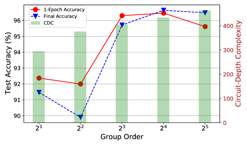
Figure 1: Cyclic Group VSA on MNIST.

To quantify the potential hardware latency of HDC, we analyze its circuit-depth complexity (CDC) in Table 2, defined as the length of the longest path from the input to the output (measured by the number of two-input gates along the path). CDC is commonly used to analyze the complexity of Boolean functions. We further assume that operations without data dependencies are all in parallel. Let $N$ be the feature vector length, e.g., $N=784$ for an MNIST image, $D$ be the hypervector dimension.

Binary HDC. The encoding stage binds all feature hypervectors, which can be implemented in a tree structure. The depth of a single binding operation (XNOR) is $1$. The total depth is therefore $\log_{2}N$. Computing the similarity includes a binding and a bit counting. We assume a B-bit ripple carry adder, a chain of full adders, has a depth of $3\cdot B$ (Satpathy, 2016). Therefore a D-bit population count has a depth of $3+6+\cdots+3\log_{2}D=\frac{3}{2}\log_{2}D\cdot(1+\log_{2}D)$.

Cyclic Group VSAs. For a cyclic group VSA of order $2^{n}$, the depth of a single binding is $3n$ as it is an addition over the group. Therefore, binding all features has a depth of $3n\log_{2}N$. For similarity computations, we precompute the similarity matrix, which consists of $\mathcal{S}(x,y),\forall x,y\in G$ in 8-bit numbers. Hence, the depth of computing the similarity for hypervectors is $3\cdot 8\cdot\log_{2}D$.

1-bit RFF perceptron. Projecting a feature vector onto a selected basis requires a depth of a 32-bit multiplier and an adder. A 32-bit Wallece tree multiplier (Wallace, 1964) has roughly a depth of 45. A 32-bit ripple carry adder has a depth of 96. A cosine operation generating random fourier features requires about the same depth as a 32-bit multiplier if computing with the CORDIC algorithm (Volder, 1959). Since the perceptron is 1-bit, computing the distance has the same depth as that of HDC.

As a result, binary HDC has a CDC of 295 on MNIST and the cyclic group G($2^{3}$) VSA has 405. The complexity of HDC is 4.4$\times$ lower than a 1-bit RFF perceptron with a depth of 1299, while CDC of the cyclic group G($2^{3}$) VSA is 3.2$\times$ lower. HDC and group VSA are much faster in potential. In Figure 1, we plot the performance and CDC of a cyclic group VSA when the order varies. Our code is available on github .

8.2 Discussion

The performance of various HDC/VSA methods is closely related to the set of its expressible similarity matrices. As a matter of fact, the required similarity matrix to learn (some) tasks in the paper might already be covered by (or close to in terms of Frobenius norm) the set of expressible similarity matrices of the $10$k-dimensional RFF HDC. Hence, the improvement from group-VSA can be limited compared to RFF HDC. If instead considering a $1$k-dimensional binary RFF HDC with a smaller set of expressible similarity matrices, group-VSA demonstrates a much better accuracy improvement. For example, on MNIST, $1$k-dimensional binary RFF HDC achieves $65.59\%$ 10-epoch test accuracy on MNIST. G($2^{3}$)-VSA, meanwhile, achieves $88.61\%$, and G($2^{4}$)-VSA achieves $92.56\%$ test accuracy.

The circuit depth serves as a preliminary analysis on the hardware complexity of HDC. While other efficient circuits, e.g., a parallel adder instead of a ripple carry adder, will have lower depth and make HDC attractive further, we avoid being over-optimistic on the estimation. For a practical hardware implementation, better circuits should be applied. Besides, circuit depth only reflects the latency. In the future, an estimation on the number of operations will reflect the energy or circuit area and will further improve the analysis.

9 Conclusion

From our theoretical analysis, there is a clear connection between the class of expressible similarity matrices and the expressivity of HDC/VSA. This new notion of expressivity reveals the limits of HDC that computes with binary hypervectors, and meanwhile provides a hint on how we can improve it. The nontrivial improvement from group VSA and the proposed techniques on HDC across various benchmarks suggests that this notion paves a new way towards the future development of HDC/VSA.

Checklist

1. For all authors…

   1. Do the main claims made in the abstract and introduction accurately reflect the paper’s contributions and scope? [Yes]

   2. Did you describe the limitations of your work? [Yes]

   3. Did you discuss any potential negative societal impacts of your work? [N/A] This work will not be likely to have negative societal impact.

   4. Have you read the ethics review guidelines and ensured that your paper conforms to them? [Yes]

2. If you are including theoretical results…

   1. Did you state the full set of assumptions of all theoretical results? [Yes]

   2. Did you include complete proofs of all theoretical results? [Yes] Due to the page limits, the complete proofs are included in the supplementary materials.

3. If you ran experiments…

   1. Did you include the code, data, and instructions needed to reproduce the main experimental results (either in the supplemental material or as a URL)? [Yes] Code and instructions are included in the supplementary materials. Datasets can be MNIST and FashionMNIST, which can be downloaded online.

   2. Did you specify all the training details (e.g., data splits, hyperparameters, how they were chosen)? [Yes] The datasplit is default to each dataset. Other details are included in the paper.

   3. Did you report error bars (e.g., with respect to the random seed after running experiments multiple times)? [No] Due to the time limit, we did not include multiple runs for each experiment.

   4. Did you include the total amount of compute and the type of resources used (e.g., type of GPUs, internal cluster, or cloud provider)? [Yes]

4. If you are using existing assets (e.g., code, data, models) or curating/releasing new assets…

   1. If your work uses existing assets, did you cite the creators? [N/A] The datasets are public. We cited the source of the data.

   2. Did you mention the license of the assets? [N/A]

   3. Did you include any new assets either in the supplemental material or as a URL? [N/A]

   4. Did you discuss whether and how consent was obtained from people whose data you’re using/curating? [N/A] The datasets are public.

   5. Did you discuss whether the data you are using/curating contains personally identifiable information or offensive content? [N/A] The datasets involved in this work do not have personal or offensive content. The content is also discussed.

5. If you used crowdsourcing or conducted research with human subjects…

   1. Did you include the full text of instructions given to participants and screenshots, if applicable? [N/A]

   2. Did you describe any potential participant risks, with links to Institutional Review Board (IRB) approvals, if applicable? [N/A]

   3. Did you include the estimated hourly wage paid to participants and the total amount spent on participant compensation? [N/A]

Appendix A Proofs of Lemmas, Statements and Theorems

Lemma 4.1.

No binary HDC can express the following similarity matrix

$$\mathbf{M}=\begin{pmatrix}1&-\frac{1}{2}&-\frac{1}{2}\\ -\frac{1}{2}&1&-\frac{1}{2}\\ -\frac{1}{2}&-\frac{1}{2}&1\\ \end{pmatrix}\;.$$

Proof.

There are $n=3$ basic entities, where we have some HDC vectors $\boldsymbol{v}_{0},\boldsymbol{v}_{1},\boldsymbol{v}_{2}\in\mathbb{R}^{D}$ which can be any dimension. We start from $D=1$ case, with the inner product as the similarity measurement, we can easily enumerate all possible similarity matrices as follows:

$$\left(\begin{smallmatrix}1&1&1\\ 1&1&1\\ 1&1&1\end{smallmatrix}\right),\;\left(\begin{smallmatrix}1&-1&1\\ -1&1&-1\\ 1&-1&1\end{smallmatrix}\right),\;\left(\begin{smallmatrix}1&1&-1\\ 1&1&-1\\ -1&-1&1\end{smallmatrix}\right),\;\left(\begin{smallmatrix}1&-1&-1\\ -1&1&1\\ -1&1&1\end{smallmatrix}\right).$$

When $D>1$, note that

$$\textstyle\mathcal{S}(\boldsymbol{v}_{i},\boldsymbol{v}_{j})=\sum_{k=1}^{D}\mathcal{S}(\boldsymbol{v}_{ik},\boldsymbol{v}_{jk})/D\;,$$

which indicates that all possible similarity matrices must reside in the convex hull of the similarity matrices enumerated above because $D$ can be of any dimension. Easy to verify that this convex hell does not contain $\mathbf{M}$: thus no binary HDC can achieve it. ∎

Statement 4.1.

Binary HDC cannot learn the following task.

Consider a supervised learning task with input example set $\mathcal{X}=\{0,1,2\}$, output label set $\mathcal{Y}=\mathcal{X}$, and source distribution

$$\mathcal{P}(x,y)=\begin{cases}1/9+2p&x=y\\ 1/9-p&x\neq y\end{cases}$$

for some small positive number $p$.

Proof.

Let $\phi:\mathcal{X}\rightarrow\{-1,1\}^{D}$ be any binary HDC encoding, and extend $\phi(x)=\phi(x\bmod 3)$ when $x>3$. Given a class $\hat{y}$, we can then compute the class representative $c_{\hat{y}}$ as

$$\begin{split}\boldsymbol{c}_{\hat{y}}&=\bigoplus_{x:y(x)=\hat{y}}\phi(x)=\operatorname*{sgn}(\operatorname*{\mathbb{E}}[\phi(x)|\hat{y}])\\ &=\operatorname*{sgn}[(\frac{1}{3}-3p)(\phi({\hat{y}+1})+\phi({\hat{y}+2}))+(\frac{1}{3}+6p)\phi(\hat{y})]\\ &=\operatorname*{sgn}[(\frac{1}{3}-3p)(\phi(\hat{y})+\phi(\hat{y}+1)+\phi(\hat{y}+2))+9p\phi(\hat{y})]\;.\end{split}$$

Note that $\phi(\hat{y})+\phi(\hat{y}+1)+\phi(\hat{y}+2)$ cannot be a zero vector; otherwise,

$$\begin{split}0&=\mathcal{S}(\phi(\hat{y}),\phi(\hat{y})+\phi(\hat{y}+1)+\phi(\hat{y}+2))\\ &=1+\sum_{j\neq\hat{y}}\mathcal{S}(\phi(\hat{y}),\phi(j)),\end{split}$$

due to symmetry, one can easily derive that $\mathcal{S}(\phi(i),\phi(j))=-1/2$ for $i\neq j$, then $\mathbf{M}$ is achieved, a contradiction to Lemma 4.1.

Since $p$ is small positive number, then the sign of $\operatorname*{\mathbb{E}}[\phi(x)|\hat{y}]$ is dominated by the first term $\phi(\hat{y})+\phi(\hat{y}+1)+\phi(\hat{y}+2)$. Hence, the class representative of class $\hat{y}$ is computed as

$$\begin{split}\boldsymbol{c}_{\hat{y}}&=\bigoplus_{x:y(x)=\hat{y}}\phi(x)=\operatorname*{sgn}(\operatorname*{\mathbb{E}}[\phi(x)|\hat{y}])\\ &=\operatorname*{sgn}(\phi(\hat{y})+\phi(\hat{y}+1)+\phi(\hat{y}+2)),\end{split}$$

which is same for each class, i.e., binary HDC fails to learn this simple task.

On the other hand, for any VSA that can express $\mathbf{M}$ with $\boldsymbol{v}_{0},\boldsymbol{v}_{1},\boldsymbol{v}_{2}$, set $\phi(x)=\boldsymbol{v}_{x}$. We can compute the class representative $c_{\hat{y}}$ as

$$\begin{split}\boldsymbol{c}_{\hat{y}}&=\bigoplus_{x:y(x)=\hat{y}}\phi(x)=\arg\max_{z}\langle z,\operatorname*{\mathbb{E}}[\phi(x)|\hat{y}]\rangle\\ &=\arg\max_{z}\langle z,(\frac{1}{3}-3p)(\phi(\hat{y})+\phi(\hat{y}+1)+\phi(\hat{y}+2))+9p\phi(\hat{y})\rangle\\ &=\arg\max_{z}\langle z,9p\phi(\hat{y})\rangle=\phi(\hat{y}).\end{split}$$

The class representative of class $\hat{y}$ will be

$$c_{\hat{y}}=\operatorname*{sgn}(\operatorname*{\mathbb{E}}[\phi(x)|\hat{y}])=\operatorname*{sgn}(\frac{3p}{2}\phi(\hat{y}))=\phi(\hat{y}),$$

which gives a Bayes optimal classifier, outputs the most probable class and proves Statement 4.2. ∎

Statement 4.2.

Any VSA (formalized in Definition $2$) that can express $\mathbf{M}_{\textup{Lemma \ref{lem:sim_hdc_fail}}}$ can learn this task.

Lemma 4.2.

Let $u_{1},u_{2},\ldots,u_{K}$ be binary vectors sampled coordinate-wise independently at random, where each coordinate of $u_{i}$ has the same probability $p_{i}$ of being $1$. Let $v_{0}$, $v_{1}$, and $v_{2}$ be vectors that result from some composition of binding and permutation acting on $u_{1},\ldots,u_{K}$, and let $\mathbf{M}\in\mathbb{R}^{3\times 3}$ be their similarity matrix, such that $\mathbf{M}_{ij}=\mathcal{S}(v_{i},v_{j})$. Then

$$\left\|\operatorname*{\mathbb{E}}[\mathbf{M}]-\begin{pmatrix}1&-\frac{1}{3}&-\frac{1}{3}\\ -\frac{1}{3}&1&-\frac{1}{3}\\ -\frac{1}{3}&-\frac{1}{3}&1\\ \end{pmatrix}\right\|_{F}\geq\frac{\sqrt{2}}{3},$$

but this target matrix is expressible by some binary HDC.

Proof.

It is straightforward to show that for some $x,y,z\in[-1,1]$

$$\mathbf{E}[\mathbf{M}]=\begin{pmatrix}1&xy&xz\\ xy&1&yz\\ xz&yz&1\\ \end{pmatrix}.$$

But since $(xy)\cdot(xz)\cdot(yz)=x^{2}y^{2}z^{2}$ is a square number, it follows that the upper-triangular elements cannot all be negative. At least one of them must be non-negative, from which the result immediately follows. A binary HDC that achieves this matrix is: $(-1,1,1)$, $(1,-1,1)$, $(1,1,-1)$. ∎

Lemma 5.1.

Suppose that $X$ and $Y$ are jointly Gaussian zero-mean unit-variance random variables. Then

$$\operatorname*{\mathbb{E}}[\operatorname*{sgn}(X)\operatorname*{sgn}(Y)]=\frac{2}{\pi}\arcsin\left(\operatorname*{\mathbb{E}}[XY]\right)$$

Proof.

Without loss of generality let $U\sim\mathcal{N}(0,I)$ be a standard Gaussian over $\mathbb{R}^{2}$, and suppose that $X=a^{T}U$, $Y=b^{T}U$ for some vectors $a,b\in\mathbb{R}^{2}$ with $\|a\|=\|b\|=1$ and $a^{T}b=\operatorname*{\mathbb{E}}[XY]$. Here, a geometric argument shows that $\operatorname*{\mathbb{P}}(X\geq 0\land Y\leq 0)=\operatorname*{\mathbb{P}}(a^{T}U\geq 0\land b^{T}U\leq 0)=\theta/(2\pi)$, where $\theta$ is the angle between $a$ and $b$. An analogous analysis of the other three cases, combined with some straightforward trigonometry, proves the lemma. ∎

Theorem 6.1.

Let $(G,\otimes)$ be a finite group, and let $X$ denote the set of its non-trivial irreducible characters. Let $\alpha:X\rightarrow\mathbb{R}_{\geq 0}$ be some function that assigns a non-negative weight to each of the characters. Then, if we set $\mathcal{S}$ to be

$$\mathcal{S}(g,h)=\frac{\sum_{\chi\in X}\alpha(\chi)\cdot\operatorname{Re}(\chi(g^{-1}\otimes h))}{\sum_{\chi\in X}\alpha(\chi)\cdot\chi(\mathbf{1})},$$

where the inverse and unit $\mathbf{1}$ are those of the group $(G,\otimes)$, and define bundling $\oplus$ as given in the definition of a group VSA, then $(G,\otimes,\mathcal{S},\oplus)$ is a finite group VSA. Any finite group VSA can be constructed in this way.

If in this construction $\alpha$ is supported on only one character $\chi$, i.e. $\mathcal{S}(g,h)=\operatorname{Re}(\chi(g^{-1}\otimes h))/\chi(\mathbf{1})$, then the VSA will have the product property.

Proof.

The first part of this theorem is a direct consequence of the following more technically-stated theorem.

The second part follows directly from the fact that if $\phi$ is an irreducible representation of a finite group $G$, and $A$ is the set of automorphisms of $G$, then for any $g\in G$,

$$\frac{1}{|A|}\sum_{a\in A}\phi(a(g))=cI$$

for some scalar $c$. In particular, this means that if $\chi$ is the corresponding character, then for any $g,h\in G$,

$$\frac{1}{|A|}\sum_{a\in A}\chi(h^{-1}a(g)) =\frac{1}{|A|}\sum_{a\in A}\operatorname{tr}\left(\phi(h^{-1})\phi(a(g))\right)$$

$$=\operatorname{tr}\left(\phi(h^{-1})\frac{1}{|A|}\sum_{a\in A}\phi(a(g))\right)$$

$$=\operatorname{tr}\left(\phi(h^{-1})\cdot cII\right)$$

$$=c\cdot\chi(h^{-1}).$$

Substituting $h=1$ yields that $c=\operatorname{Re}(\chi(g))/\chi(1)$ (since $\chi$ must also be preserved by automorphisms up to complex conjugation), which immediately implies what we wanted to prove. ∎

Theorem A.1 (Representation theorem for group VSAs).

Suppose that we have a finite group $G$ equipped with a similarity measure denoted $\langle\cdot|\cdot\rangle_{G}$. Let $X$ denote the set of non-trivial irreducible characters of $G$ (i.e. $X$ is the character table of $G$ excluding the top row). Then there exists a unique function $\alpha:X\rightarrow\mathbb{R}_{\geq 0}$ such that $\alpha(\bar{\chi})=\alpha(\chi)$ for all $\chi\in X$, $\sum_{\chi\in X}\alpha(\chi)\cdot\chi(1)=1$, and

$$\langle\cdot|\cdot\rangle_{G}=\sum_{\chi\in X}\alpha(\chi)\cdot\chi(g^{-1}h).$$ (2)

Conversely, for any function $\alpha$ of this type, if we define $\langle\cdot|\cdot\rangle$ according to (2), then $\langle\cdot|\cdot\rangle$ will be a similarity measure for $G$.

Additionally, if we define $M$ as the matrix such that $M_{gh}=\langle g|h\rangle_{G}$, and $d$ is the rank of $M$, then there exists some positive integer $K$ and positive integers $d_{1},d_{2},\ldots,d_{K}$ such that $\sum_{k=1}^{K}d_{K}=1$, and there exists a $|G|$-dimensional subspace $\mathcal{A}$ of $\mathbb{R}^{d_{1}\times d_{1}}\times\mathbb{R}^{d_{2}\times d_{2}}\times\cdots\times\mathbb{R}^{d_{K}\times d_{K}}$ and function $\phi:G\rightarrow\mathcal{A}$ such that for all $g,h\in G$,

$$\phi(g)\phi(h) =\phi(gh)$$

$$\phi(g)^{-1}=\phi(g)^{T} =\phi(g^{-1})$$

$$\phi(1) =\phi(I),$$

where multiplication and transposition in $\mathcal{A}$ is done component-wise on the $K$ components (each of which is a matrix), and such multiplication preserves $\mathcal{A}$. Also, there exist some positive scalars $\beta_{1},\beta_{2},\ldots,\beta_{K}$ such that if we define an inner product on $\mathcal{A}$ as

$$\langle(x_{1},x_{2},\ldots,x_{K}),(y_{1},y_{2},\ldots,y_{K})\rangle_{\mathcal{A}}=\sum_{k=1}^{K}\beta_{k}\operatorname{tr}\left(x_{k}^{T}y_{k}\right),$$

where here each $x_{k}\in\mathbb{R}^{d_{k}\times d_{k}}$, then

$$\langle g|h\rangle_{G}=\langle\phi(g)|\phi(h)\rangle_{\mathcal{A}}.$$

Proof.

Let $M$ be the matrix described in the theorem statement, such that $M_{gh}=\langle g|h\rangle_{G}$. Observe that $M$ must be symmetric and positive semidefinite (by the properties of the similarity measure). For some $f\in G$, let $B_{f}$ denote the matrix

$$B_{f}=\sum_{g\in G}e_{fg}e_{g}^{T},$$

where $e_{g}$ is the unit basis element associated with $g$. Observe that $B_{f}^{T}=B_{f}^{-1}=B_{f^{-1}}$, and that $B_{f}$ commutes with $M$, because

$$e_{h}^{T}MB_{f}e_{g} =e_{h}^{T}Me_{fg}$$

$$=\rho(h^{-1}fg)$$

$$=\rho((f^{-1}h)^{-1}g)$$

$$=e_{f^{-1}h}^{T}Me_{g}$$

$$=\left(B_{f^{-1}}e_{h}\right)^{T}Me_{g}$$

$$=e_{h}^{T}B_{f^{-1}}^{T}Me_{g}$$

$$=e_{h}^{T}B_{f}Me_{g}.$$

That is, $MB_{f}=B_{f}M$. Since $B_{f}$ commutes with $M$, it also must commute with any polynomial of $M$. In particular, if the nonzero eigendecomposition of $M$ is

$$M=\sum_{k=1}^{K}\lambda_{k}V_{k},$$

where each $\lambda_{k}>0$ is distinct, and $V_{k}^{2}=V_{k}$ is a symmetric projection matrix onto the associated eigenspace, then since $V_{k}$ can be expressed as a polynomial in $M$, it must also commute with $B_{f}$ for all $f$. The same thing will be true for $C_{f}$ defined as

$$C_{f}=\sum_{g\in G}e_{gf}e_{g}^{T}.$$

These results together show that for any $f,g,h\in G$,

$$e_{h}^{T}V_{k}e_{g}=e_{fh}^{T}V_{k}e_{fg}=e_{hf}^{T}V_{k}e_{gf}.$$

Now, let $d_{k}$ denote the rank of $V_{k}$ (the multiplicity of the eigenvalue $\lambda_{k}$ in $M$). So, there must exist some matrix $W_{k}\in\mathbb{R}^{|G|\times d_{k}}$ such that $V_{k}=W_{k}W_{k}^{T}$ and $W_{k}^{T}W_{k}=I$. For any $g\in G$, let $U_{k}(g)$ denote the matrix in $\mathbb{R}^{d_{k}\times d_{k}}$

$$U_{k}(g)=W_{k}^{T}B_{g}W_{k}.$$

Observe that $U_{k}(1)=I$, all the $U_{k}(g)$ matrices are orthogonal, and

$$U_{k}(g)U_{k}(h) =W_{k}^{T}B_{g}W_{k}W_{k}^{T}B_{h}W_{k}$$

$$=W_{k}^{T}B_{g}V_{k}B_{h}W_{k}$$

$$=W_{k}^{T}B_{g}B_{h}V_{k}W_{k}$$

$$=W_{k}^{T}B_{gh}W_{k}$$

$$=U_{k}(gh).$$

That is, $U_{k}$ is a representation of the group $G$. Observe that the trace of $U_{k}(g)$ is

$$\operatorname{tr}\left(U_{k}(g)\right) =\operatorname{tr}\left(W_{k}^{T}B_{g}W_{k}\right)$$

$$=\operatorname{tr}\left(W_{k}W_{k}^{T}B_{g}\right)$$

$$=\operatorname{tr}\left(V_{k}B_{g}\right)$$

$$=\sum_{h\in G}e_{h}^{T}V_{k}B_{g}e_{h}$$

$$=\sum_{h\in G}e_{h}^{T}V_{k}e_{gh}$$

$$=\sum_{h\in G}e_{1}^{T}V_{k}e_{g}$$

$$=|G|\cdot e_{1}^{T}V_{k}e_{g}.$$

In particular, this means that $g\mapsto|G|\cdot e_{1}^{T}V_{k}e_{g}$ is a character of $G$. As a character, it must be a sum of irreducible characters of $G$, and since it is real, it must place the same weight on complex-conjugate characters. It follows that $g\mapsto\sum_{k=1}^{K}\lambda_{k}e_{1}^{T}V_{k}e_{g}$ must be a non-negative scaled sum of irreducible characters of $G$ that places the same weight on complex-conjugate characters. But, this function is just $g\mapsto e_{1}^{T}Me_{g}$, which is just $\rho$. So, $\rho$ must be a non-negative sum of the irreducible characters of $G$. The fact that this scaling is unique follows from the fact that the characters are linearly independent; the fact that this scaling only contains non-trivial characters follows from the average-dissimilarity property.

We then construct an algebra $\mathcal{A}$ as follows. Let $\phi(g):G\rightarrow\mathbb{R}^{d_{1}\times d_{1}}\times\cdots\times R_{d_{K}\times d_{K}}$ be defined as

$$\phi(g)=(U_{1}(g),U_{2}(g),\ldots,U_{K}(g)),$$

and let the inner product scalars be

$$\beta_{k}=\frac{\lambda_{k}}{|G|}.$$

Then

$$\sum_{k=1}^{K}\beta_{k}\operatorname{tr}\left(U_{k}(h)^{T}U_{k}(g)\right) =\sum_{k=1}^{K}\beta_{k}\operatorname{tr}\left(U_{k}(h^{-1})U_{k}(g)\right)$$

$$=\sum_{k=1}^{K}\beta_{k}\operatorname{tr}\left(U_{k}(h^{-1}g)\right)$$

$$=e_{1}^{T}Me_{h^{-1}g}$$

$$=\rho(h^{-1}g)$$

$$=\langle h|g\rangle_{G}$$

as desired. To finish the construction, let $\mathcal{A}$ be the algebra spanned by $\{\phi(g)\mid g\in G\}$. Observe that this must be closed under multiplication and transposition because $G$ is closed under multiplication and inversion. ∎

Statement 6.1.

Let $\mathbf{M}$ be similarity matrices expressible by a finite group VSA. Then there exists a finite group VSA that has the product property and can also achieve $\mathbf{M}$.

Proof.

Suppose the first VSA’s group is $G$ and has irreducible characters $\chi_{1},\chi_{2},\ldots,\chi_{k}$. Then the group $G^{k}$ consisting of the direct product of $k$ copies of the group $G$, together with a similarity function $\mathcal{S}((x_{1},\ldots,x_{k}),(y_{1},\ldots,y_{k}))\propto\prod_{i=1}^{k}\chi_{i}(x_{i}^{-1}\otimes y_{i})$ will both have the product property (as its similarity matrix is proportional to a single character) and can express any similarity matrix the first VSA can. ∎

Statement 6.2.

Any similarity matrix $\mathbf{M}$ that can be expressed by a finite Abelian group VSA can be expressed by the unit-cycle VSA ($G=\{z\in C\mid|z|=1\}$, $x\otimes y=xy$, $\mathcal{S}(x,y)=\operatorname{Re}(x^{*}y)$).

Proof.

Note the fact that all irreducible representations of finite Abelian groups are 1-dimensional. Then the results follows immediately with any irreducible representation as the mapping from a finite Abelian group to $G=\{z\in C\mid|z|=1\}$. ∎

Statement 6.3.

There exists a similarity matrix $\mathbf{M}$ that can be expressed by a VSA over the (non-Abelian) binary icosahedral group, but not by the unit-cycle VSA.

Proof.

Consider the binary icosahedral group expressed as a subset of the quaternions. This group consists of 120 elements which are placed at the vertices of a 600-cell inscribed in the unit 3-sphere. Consider an arbitrary sequence of 60 of these elements containing exactly one of $\{x,-x\}$ for each $x$ in the binary icosahedral group: i.e. we select exactly one of each pair of antipodal points in the group. This sequence of 60 points has a similarity matrix $M\in\mathbb{R}^{60\times 60}$. It is easy to check that the absolute values of the entries of this matrix lie in $\{0,\frac{1}{2\phi},\frac{1}{2},\frac{\phi}{2},1\}$, where $\phi=\frac{1+\sqrt{5}}{2}$ is the golden ratio. Define the matrix $A\in\mathbb{R}^{60\times 60}$ such that $A_{ij}=\pm 1$ if $M_{ij}=\pm\frac{\phi}{2}$ and $A_{ij}=0$ otherwise. Consider the optimization problem to maximize $\operatorname{tr}(AZ)$ over positive semidefinite matrices $Z\in\mathbb{R}^{60\times 60}$ subject to the constraint that the diagonal of $Z$ is all-ones, i.e. $Z_{ii}=1$. It is easy to check numerically that the only solution to this optimization problem is $Z=M$. Also observe that $M$ has rank greater than $2$.

Now, suppose that there existed some representation of $M$ using vectors with entries in the unit circle in $\mathbb{C}$. For this to hold, it would need to be the case that $M$ is in the convex combination of the similarity matrices generated by those entries, each of which must be of rank $2$. But, this is impossible, since (1) none of those matrices can be equal to $M$, and as such (2) any such matrix $M_{C}$ will have $\operatorname{tr}(M_{C}A)<\operatorname{tr}(MA)$. This shows that this particular matrix can’t be represented by hypervectors with unit-absolute-value entries in $\mathbb{C}$. ∎

Appendix B Calculation of $\theta$ in Section 7

We can theoretically calculate the angle $\theta$ between the class vector $s_{c}$ and a randomly selected hypervector $t_{i}$ in the set $\mathbb{T}_{c}$.

$$\text{cos}\theta=\frac{s_{c}\cdot v_{j}}{\left\|s_{c}\right\|\left\|v_{j}\right\|}=\frac{2\cdot q-D}{D}$$

$D$ is the dimension of $t_{i}$. $q$ is the number of elements that have the same sign in $s_{c}$ and $t_{i}$. Since

$$s_{c}=\text{sgn}\left(\bigoplus_{j\in\mathbb{T}_{c}}t_{j}\right)=\text{sgn}\left(t_{i}+\sum_{j=1,j\neq i}^{2k+1}t_{j}\right)\;,$$

$q$ is proportional to the probability $p_{k}$ of the sign of an entry in $t_{i}$ will be flipped after adding the term $\sum_{j=1,j\neq i}^{2k+1}t_{j}$ (the other $2k$ vectors) to it. Obviously $q=D\cdot p_{k}$ as each entry in $t_{i}$ is independent.

In order to avoid flipping the sign of an entry, there should be at least $k$ entries out of $2k$ that have the same sign, so the probability $p_{k}$ can be calculated by

$$p_{k}=\frac{\binom{2k}{k}+\binom{2k}{k+1}+\cdots+\binom{2k}{2k}}{2^{2k}}=\frac{1+\frac{1}{2^{2k}}\binom{2k}{k}}{2}$$

Plug the expression of $p_{k}$ into $\text{cos}\theta$, we can get

$$\theta_{2k+1}=\text{cos}^{-1}(\frac{1}{2^{2k}}\cdot\binom{2k}{k})$$

Importantly, $p_{k}$ is monotonic.

Proof.

$$p_{k+1} =\frac{1+\frac{1}{2^{2k}}\cdot\frac{1}{4}\cdot{2k+2\choose k+1}}{2}$$

$$=\frac{1+\frac{1}{2^{2k}}\cdot\frac{1}{4}\cdot[{2k+1\choose k+1}+{2k+1\choose k}]}{2}$$

$$=\frac{1+\frac{1}{2^{2k}}\cdot\frac{1}{4}\cdot[{2k\choose k+1}+{2k\choose k}+{2k\choose k}+{2k\choose k-1}]}{2}$$

$$<\frac{1+\frac{1}{2^{2k}}\cdot\frac{1}{4}\cdot 4\cdot{2k\choose k}}{2}$$

$$=p_{k}$$

∎

This means that the more vectors we bundle together, the closer $\theta$ is to 90 degrees.

Appendix C Learning with Group VSA

For a cyclic group VSA model, similar as the binary HDC case, we initialize a linear model with weights $\mathbf{W}$ of size $\#\operatorname{class}\times D$, where each element belongs to $G=\mathbb{Z}/n\mathbb{Z}=\{0,1,\cdots,n-1\}$. Inputs to this classifier are encoded hypervectors $v\in G^{D}$, the model computes per-class similarities with defined similarity function:

$$\mathcal{S}(x,y)=\langle\psi(x),\psi(y)\rangle=\cos(2\pi(x-y)/n),\forall x,y\in G,$$

which extends to higher dimensional space via

$$\mathcal{S}([x_{1},\ldots,x_{D}],[y_{1},\ldots,y_{D}])=\frac{1}{D}\sum_{i=1}^{D}\mathcal{S}(x_{i},y_{i}).$$

We calculate the cross-entropy loss between the classifier outputs and the labels, and do back propagation using high precision numbers such as $16$-bit floats. At each optimizer step, SGD optimizer moves $\mathbf{W}$ away from $G^{\#\operatorname{class}\times D}$, we pull it back with (Fast)-Round operation to finish current step before entering next step. Similar as the binary case, the inference cost remains the same as the bundling method.

References

- Anguita et al. (2012) Davide Anguita, Alessandro Ghio, Luca Oneto, Xavier Parra, and Jorge L. Reyes-Ortiz. Human activity recognition on smartphones using a multiclass hardware-friendly support vector machine. In José Bravo, Ramón Hervás, and Marcela Rodríguez, editors, Ambient Assisted Living and Home Care, pages 216–223. Springer Berlin Heidelberg, 2012.
- Basaklar et al. (2021) Toygun Basaklar, Yigit Tuncel, Shruti Yadav Narayana, Suat Gumussoy, and Umit Y. Ogras. Hypervector design for efficient hyperdimensional computing on edge devices. In Research Symposium on Tiny Machine Learning, 2021. URL https://openreview.net/forum?id=JGNDej3tup9.
- Burrello et al. (2019) Alessio Burrello, Lukas Cavigelli, Kaspar Schindler, Luca Benini, and Abbas Rahimi. Laelaps: An energy-efficient seizure detection algorithm from long-term human ieeg recordings without false alarms. In 2019 Design, Automation and Test in Europe Conference and Exhibition (DATE), pages 752–757, 2019. doi: 10.23919/DATE.2019.8715186.
- Chuang et al. (2020) Yu-Chuan Chuang, Cheng-Yang Chang, and An-Yeu Andy Wu. Dynamic hyperdimensional computing for improving accuracy-energy efficiency trade-offs. In 2020 IEEE Workshop on Signal Processing Systems (SiPS), pages 1–5, 2020.
- Dua and Graff (2017) Dheeru Dua and Casey Graff. UCI machine learning repository, 2017. URL http://archive.ics.uci.edu/ml.
- Frady et al. (2018) E Paxon Frady, Denis Kleyko, and Friedrich T Sommer. A theory of sequence indexing and working memory in recurrent neural networks. Neural Computation, 30(6):1449–1513, 2018.
- Frady et al. (2021) E. Paxon Frady, Denis Kleyko, Christopher J. Kymn, Bruno A. Olshausen, and Friedrich T. Sommer. Computing on functions using randomized vector representations, 2021.
- Fulton and Harris (2013) William Fulton and Joe Harris. Representation theory: a first course, volume 129. Springer Science & Business Media, 2013.
- Gallant and Okaywe (2013) Stephen I. Gallant and T. Wendy Okaywe. Representing Objects, Relations, and Sequences. Neural Computation, 25(8):2038–2078, 08 2013. ISSN 0899-7667. doi: 10.1162/NECO_a_00467.
- Gayler (1998) Ross W Gayler. Multiplicative binding, representation operators & analogy (workshop poster). 1998.
- Ge and Parhi (2020) Lulu Ge and Keshab K. Parhi. Classification using hyperdimensional computing: A review. IEEE Circuits and Systems Magazine, 20(2):30–47, 2020. ISSN 1558-0830. doi: 10.1109/mcas.2020.2988388. URL http://dx.doi.org/10.1109/MCAS.2020.2988388.
- Gosmann and Eliasmith (2019) Jan Gosmann and Chris Eliasmith. Vector-Derived Transformation Binding: An Improved Binding Operation for Deep Symbol-Like Processing in Neural Networks. Neural Computation, 31(5):849–869, 05 2019. ISSN 0899-7667. doi: 10.1162/neco_a_01179. URL https://doi.org/10.1162/neco_a_01179.
- Guo et al. (2021) Yunhui Guo, Mohsen Imani, Jaeyoung Kang, Sahand Salamat, Justin Morris, Baris Aksanli, Yeseong Kim, and Tajana Rosing. Hyperrec: Efficient recommender systems with hyperdimensional computing. In Proceedings of the 26th Asia and South Pacific Design Automation Conference, ASPDAC ’21, page 384–389. Association for Computing Machinery, 2021. ISBN 9781450379991. doi: 10.1145/3394885.3431553.
- Gupta et al. (2020) Saransh Gupta, Justin Morris, Mohsen Imani, Ranganathan Ramkumar, Jeffrey Yu, Aniket Tiwari, Baris Aksanli, and Tajana Rosing. Thrifty: Training with hyperdimensional computing across flash hierarchy. In 2020 IEEE/ACM International Conference On Computer Aided Design (ICCAD), pages 1–9, 2020.
- Hernandez-Cane et al. (2021) Alejandro Hernandez-Cane, Namiko Matsumoto, Eric Ping, and Mohsen Imani. Onlinehd: Robust, efficient, and single-pass online learning using hyperdimensional system. In 2021 Design, Automation and Test in Europe Conference and Exhibition (DATE), pages 56–61, 2021. doi: 10.23919/DATE51398.2021.9474107.
- Hopfield (1982) J J Hopfield. Neural networks and physical systems with emergent collective computational abilities. Proceedings of the National Academy of Sciences, 79(8):2554–2558, 1982. ISSN 0027-8424. doi: 10.1073/pnas.79.8.2554. URL https://www.pnas.org/content/79/8/2554.
- Hubara et al. (2016) Itay Hubara, Matthieu Courbariaux, Daniel Soudry, Ran El-Yaniv, and Yoshua Bengio. Binarized neural networks. In Advances in Neural Information Processing Systems, 2016.
- Imani et al. (2019a) Mohsen Imani, John Messerly, Fan Wu, Wang Pi, and Tajana Rosing. A binary learning framework for hyperdimensional computing. In 2019 Design, Automation and Test in Europe Conference and Exhibition (DATE), pages 126–131, 2019a. doi: 10.23919/DATE.2019.8714821.
- Imani et al. (2019b) Mohsen Imani, Justin Morris, John Messerly, Helen Shu, Yaobang Deng, and Tajana Rosing. Bric: Locality-based encoding for energy-efficient brain-inspired hyperdimensional computing. In Proceedings of the 56th Annual Design Automation Conference 2019, pages 1–6, 2019b.
- Imani et al. (2020) Mohsen Imani, Saikishan Pampana, Saransh Gupta, Minxuan Zhou, Yeseong Kim, and Tajana Rosing. Dual: Acceleration of clustering algorithms using digital-based processing in-memory. In 2020 53rd Annual IEEE/ACM International Symposium on Microarchitecture (MICRO), pages 356–371, 2020. doi: 10.1109/MICRO50266.2020.00039.
- Imani et al. (2021) Mohsen Imani, Zhuowen Zou, Samuel Bosch, Sanjay Anantha Rao, Sahand Salamat, Venkatesh Kumar, Yeseong Kim, and Tajana Rosing. Revisiting hyperdimensional learning for fpga and low-power architectures. In 2021 IEEE International Symposium on High-Performance Computer Architecture (HPCA), pages 221–234, 2021. doi: 10.1109/HPCA51647.2021.00028.
- James et al. (2001) Gordon James, Martin W Liebeck, and Martin Liebeck. Representations and characters of groups. Cambridge University Press, 2001.
- Kanerva (1994) Pentti Kanerva. The spatter code for encoding concepts at many levels. In International Conference on Artificial Neural Networks, pages 226–229. Springer, 1994.
- Kanerva (2009) Pentti Kanerva. Hyperdimensional computing: An introduction to computing in distributed representation with high-dimensional random vectors. Cogn. Comput., pages 139–159, 2009.
- Kanerva et al. (1997) Pentti Kanerva et al. Fully distributed representation. PAT, 1(5):10000, 1997.
- Kim et al. (2020) Yeseong Kim, Mohsen Imani, Niema Moshiri, and Tajana Rosing. Geniehd: Efficient dna pattern matching accelerator using hyperdimensional computing. In 2020 Design, Automation and Test in Europe Conference and Exhibition (DATE), pages 115–120, 2020. doi: 10.23919/DATE48585.2020.9116397.
- Kleyko et al. (2016) Denis Kleyko, Evgeny Osipov, Alexander Senior, Asad I Khan, and Yaşar Ahmet Şekerciogğlu. Holographic graph neuron: A bioinspired architecture for pattern processing. IEEE transactions on neural networks and learning systems, 28(6):1250–1262, 2016.
- Lecun et al. (1998) Y. Lecun, L. Bottou, Y. Bengio, and P. Haffner. Gradient-based learning applied to document recognition. Proceedings of the IEEE, 86(11):2278–2324, 1998.
- Mitrokhin et al. (2019) A. Mitrokhin, P. Sutor, C. Fermüller, and Y. Aloimonos. Learning sensorimotor control with neuromorphic sensors: Toward hyperdimensional active perception. Science Robotics, 4(30):eaaw6736, 2019. doi: 10.1126/scirobotics.aaw6736.
- Neubert and Schubert (2021) Peer Neubert and Stefan Schubert. Hyperdimensional computing as a framework for systematic aggregation of image descriptors, 2021.
- Neubert et al. (2019) Peer Neubert, Stefan Schubert, and Peter Protzel. An introduction to hyperdimensional computing for robotics. KI - Künstliche Intelligenz, 33, 09 2019. doi: 10.1007/s13218-019-00623-z.
- Plate (1995) T.A. Plate. Holographic reduced representations. IEEE Transactions on Neural Networks, 6(3):623–641, 1995. doi: 10.1109/72.377968.
- Plate (1994) Tony A Plate. Distributed representations and nested compositional structure. Citeseer, 1994.
- Rahimi and Recht (2007) Ali Rahimi and Benjamin Recht. Random features for large-scale kernel machines. In Proceedings of the 20th International Conference on Neural Information Processing Systems, NIPS’07, page 1177–1184, 2007. ISBN 9781605603520.
- Rosenblatt (1958) Frank Rosenblatt. The perceptron: a probabilistic model for information storage and organization in the brain. Psychological review, 65(6):386, 1958.
- Salamat et al. (2019) Sahand Salamat, Mohsen Imani, Behnam Khaleghi, and Tajana Rosing. F5-hd: Fast flexible fpga-based framework for refreshing hyperdimensional computing. In Proceedings of the 2019 ACM/SIGDA International Symposium on Field-Programmable Gate Arrays, FPGA ’19, page 53–62. Association for Computing Machinery, 2019. ISBN 9781450361378. doi: 10.1145/3289602.3293913.
- Satpathy (2016) Pinaki Satpathy. Design and Implementation of Carry Select Adder Using T-Spice. Anchor Academic Publishing, 2016.
- Schlegel et al. (2021) Kenny Schlegel, Peer Neubert, and Peter Protzel. A comparison of vector symbolic architectures. Artificial Intelligence Review, Dec 2021. ISSN 1573-7462. doi: 10.1007/s10462-021-10110-3. URL http://dx.doi.org/10.1007/s10462-021-10110-3.
- Serre (1977) Jean-Pierre Serre. Linear representations of finite groups, volume 42. Springer, 1977.
- Smith and Stanford (1990) Derek Smith and Paul Stanford. A random walk in hamming space. In 1990 IJCNN International Joint Conference on Neural Networks, pages 465–470. IEEE, 1990.
- Thomas et al. (2020) Anthony Thomas, Sanjoy Dasgupta, and Tajana Rosing. Theoretical foundations of hyperdimensional computing, 2020.
- Vert et al. (2004) Jean-Philippe Vert, Koji Tsuda, and Bernhard Schölkopf. A primer on kernel methods. Kernel methods in computational biology, 47:35–70, 2004.
- Volder (1959) Jack E. Volder. The cordic trigonometric computing technique. IRE Transactions on Electronic Computers, EC-8(3):330–334, 1959. doi: 10.1109/TEC.1959.5222693.
- Wallace (1964) C. S. Wallace. A suggestion for a fast multiplier. IEEE Transactions on Electronic Computers, EC-13(1):14–17, 1964. doi: 10.1109/PGEC.1964.263830.
- Xiao et al. (2017) Han Xiao, Kashif Rasul, and Roland Vollgraf. Fashion-mnist: a novel image dataset for benchmarking machine learning algorithms, 2017.