Abstract: Rapid technological advances have allowed for molecular profiling across multiple omics domains from a single sample for clinical decision making in many diseases, especially cancer. As tumor development and progression are dynamic biological processes involving composite genomic aberrations, key challenges are to effectively assimilate information from these domains to identify genomic signatures and biological entities that are druggable, develop accurate risk prediction profiles for future patients, and identify novel patient subgroups for tailored therapy and monitoring.
We propose integrative probabilistic frameworks for high-dimensional multiple-domain cancer data that coherently incorporate dependence within and between domains to accurately detect tumor subtypes, thus providing a catalogue of genomic aberrations associated with cancer taxonomy. We propose an innovative, flexible and scalable Bayesian nonparametric framework for simultaneous clustering of both tumor samples and genomic probes. We describe an efficient variable selection procedure to identify relevant genomic aberrations that can potentially reveal underlying drivers of a disease. Although the work is motivated by several investigations related to lung cancer, the proposed methods are broadly applicable in a variety of contexts involving high-dimensional data. The success of the methodology is demonstrated using artificial data and lung cancer omics profiles publicly available from The Cancer Genome Atlas.

1 Introduction

An overarching goal of cancer omics studies is identifying patient profiles based on various genetic and epigenetic aberrations in tumors (Simon and Roychowdhury, 2013; Navin, 2014; Wang et al., 2018). Rapid technological advances in recent years have enabled molecular profiling of patients across multiple omics domains, such as SNP, mRNA, gene and protein expression. In the past, studies have typically analyzed the somatic measurements one domain at a time with some degree of success. For example, high-resolution RNA sequencing and microRNA profiling have led to the discovery of novel cancer molecular subtypes in bladder cancer (Choi et al., 2017) and breast cancer (Haakensen et al., 2016). However, as tumor development and progression involve complex genomic aberrations occurring across multiple domains, it is important, although statistically challenging, to effectively assimilate information across the domains to accurately identify biological entities, genomic signatures, and risk prediction profiles for the patients. This is especially true of “small $n$, large $p$” problems where the number of biomarkers overwhelms the number of patients.

1.1 Motivating application

The Cancer Genome Atlas (TCGA) is a worldwide project that focuses on cataloging genetic mutations responsible for various cancers (https://www.cancer.gov/about-nci/organization/ccg/research/structural-genomics/tcga). Currently, TCGA characterizes more than 30 cancer types, including 10 rare cancers. The advent of TCGA has further incentivized the integration of data from multiple domains to identify meaningful and druggable biomarkers associated with tumor development and progression.

Lung cancer is the second most common cancer in both men and women in the US, to date accounting for more than 235,760 new cases and 131,880 deaths in 2021 (https://www.cancer.org/cancer/lung-cancer/about/key-statistics.html). It is the number one cause of cancer death among men and women, constituting almost 25% of all cancer deaths. Lung adenocarcinoma (LUAD) and lung squamous cell carcinoma (LUSC) are the two major subtypes of non-small cell lung cancer (NSCLC), which accounts for more than 80% of all lung cancers (Singh et al., 2020). A comprehensive genomic profiling on LUSC and LUAD tumor samples has been studied in Cancer Genome Atlas Research Network (2014, 2012). Although we focus on the integrative analysis of gene expression and DNA methylation data in Section 4.2, but the proposed methodology is applicable to an arbitrary number of platforms.

1.2 Existing methods

Existing integrative methods can be categorized into four groups based on the main study goals. The first group involves one-at-a-time analysis of heterogeneous data from different platforms to validate biological assumptions. These studies obtain data from one platform, analyze it along with outcomes of interest, and then perform a similar analysis using a different platform for the purpose of validating the results of the previous analysis. For example, Cenik et al. (2015) used ribosome occupancy maps coupled with previously measured RNA expression and protein levels from the same group of individuals to improve the identification of disease risk factors. Lian et al. (2019) obtained one stemness index from gene expression, another stemness index from DNA methylation for verification, and observed an inverse trend between them for metastatic status.

The second group of studies focuses on the discovery and characterization of biological pathways or regulatory mechanisms associated with the disease. For example, Wu et al. (2018) studied the associations among DNA methylation and phenotype for follow-up functional studies to reveal complex disease traits. Yoo et al. (2019) and Fan et al. (2019) performed integrative analyses of two or more omics platforms to detect possible signaling pathways related to the progression of different cancers.

The third group of studies aim to capture biological heterogeneity from various platforms to detect sparse subsets of informative variables that predict clinical outcomes. For example, Wang et al. (2013) proposed a hierarchical model to capture the natural mechanistic relationships among multi-platform genomic data, thereby detecting disease-related genes with higher power than each platform individually. Yang et al. (2017) collectively model multi-omics platforms with an unsupervised Bayesian nonparametric framework to identify driver genes. An integrative approach for biomarker discovery using latent components coupled with supervised analysis and prediction has been implemented by Singh et al. (2019). Maity et al. (2020), on the other hand, predicted patients’ prognosis from their molecular profiles with a Bayesian structural equation modeling.

The fourth group of studies concerns integrative clustering of subjects to detect biologically relevant subpopulations. These approaches typically model latent components or specify similarity scores among subjects to detect clusters of patients potentially corresponding to disease subtypes. Lock and Dunson (2013) proposed Bayesian consensus clustering (BCC), which gives an overall clustering of data sources, also allows source-specific clustering. However, misspecifying the number of clusters could easily lead to under or over fitting. Dependence of each platform to the overall clustering is always difficult to justify as well, for the reason that the parameters which control the adherence of platform to the overall clustering depend on number of clusters; the strength of adherence is therefore hard to specify or learn. The iCluster methods (Mo et al., 2018, 2013; Shen et al., 2009) used orthogonal latent variables to represent complex molecular structures, achieving dimension reduction and revealing tumor subtypes. Many other integrative clustering techniques focus on optimizing survival curves separation while simultaneously detecting patients groups with similar molecular traits (Ahmad and Fröhlich, 2017; Coretto et al., 2018). Park et al. (2021) recently proposed a kernel-learning method that utilizes the spectral clustering framework with a flexible choice of similarity measure to detect cancer patient subtypes.

2 Approach

The central hypothesis behind our proposed approach is that multiple omics platforms provide contrasting, yet intrinsically interrelated, information about the underlying molecular drivers of phenotypes or clinical outcomes. Consequently, to improve tailored therapy and monitoring for cancer patients, it is crucial to aggregate information from the platforms to uncover novel patient subpopulations, e.g., cancer subtypes, and quantify the associations of the somatic measurements with the study endpoints. The challenges posed by these integrative analyses include not only high dimensionality, but also substantial probe-to-probe dependencies caused by complex biomarker interactions through gene or metabolic pathways.

To tackle these challenges, we propose a flexible Bayesian nonparametric framework for analyzing multi-domain, complexly structured, and high throughput modern array data and detecting different biological structures in different platforms. The model that can be summarized as follows. We utilize the flexibility of Poisson-Dirichlet processes (PDPs) to discover the biological dependence of the multivariate vectors associated with the biomarkers, both within and between the omics domains. The PDPs naturally facilitate dimension reduction in the large number of omics biomarkers, allowing variable selection in these high-dimensional settings, and providing a catalogue of genomic aberrations associated with the cancer-related clinical outcomes. A nested univariate Dirichlet process induces an overall, global clustering of the patients across the disparate data sources to detect an unknown number of tumor subtypes. The MCMC procedure for fitting the model is computationally feasible due to the application of data-squashing techniques developed in Guha (2010) that drastically reduce the computational times for high-throughput omics datasets.

The rest of the paper is organized as follows. Section 3.1 introduces the details of the integrative Bayesian hierarchical model in three major parts. Specifically, Section 3.1.1 introduces a novel bidirectional clustering technique that achieves nonparametric dimension reduction and platform-specific detection of unknown pathways. In Section 3.1.2, we propose a method to account for the similarity of the elements of platform within each unsupervised bidirectional cluster. Section 3.1.3 discusses a similar hierarchical construction of Teh et al. (2006) that allows the borrowing of strength within and across platforms. Section 3.2 describes a variable selection procedure that can effectively filter useful information about any available clinical outcome to improve the quality and stability of the subtypes discovery. Posterior inference procedures are illustrated in Section 3.3. Through simulations in Section 4.1, we demonstrate the accuracy of the clustering mechanism using simulated datasets. In Section 4.2, we analyze the motivating gene expression and DNA methylation datasets for lung cancer. We conclude with some remarks in Section 5.

3 Methods

3.1 An Integrative Bayesian Hierarchical Model for Multiple Omics Domains

As the same patient tumor samples are profiled using different assays, the data are inherently dependent across the various platforms. We develop a statistical framework for the joint modeling of discrete and continuous somatic measurements arising from multiple omics domains. We begin with some basic notation. Assume that we wish to analyze $T\geq 2$ platforms or omics datasets for a total of $n$ matched patients or tissue samples for a certain disease. In general, the observations for a given platform may be continuous (e.g., gene expression data), count (e.g., copy number variation data), or proportion (e.g., DNA methylation data).

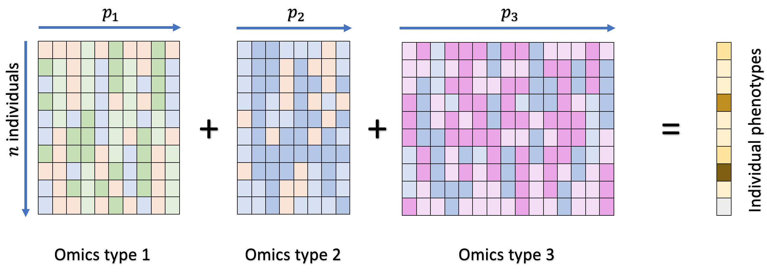
Figure 1: A graphical illustration of data structure: $n$ individuals measured at $T=3$ platforms whose survival time and censoring indicator are recorded as clinical outcomes.

Let $\bm{X}_{t}$ represent the matrix of genomic or epigenomic measurements associated with the $t$th platform. The rows of matrix $\bm{X}_{t}$ represent the $n$ patients, and the matrix columns represent the $p_{t}$ biomarkers. Although $n$ itself is fairly large, it is typically far smaller than the number of biomarkers in each dataset, so that $n\ll\min_{t}p_{t}$. A generic element of matrix $\bm{X}_{t}$ is $X_{ijt}$ for row (patient) $i=1,2,\dots,n$, and column (probe) $j=1,2,\dots,p_{t}$. Patient phenotypes, such as overall survival times, are denoted by $w_{i}$ for $i=1,\cdots,n$. See Figure 1 for a graphical representation. With $t_{i}$ denoting the failure time and $C_{i}$ denoting the independent censoring time, the observed survival time $w_{i}=\min\{t_{i},C_{i}\}$ and censoring indicator $\Delta_{i}=\mathcal{I}(t_{i}\leq C_{i})$.

3.1.1 Bidirectional clusters: dimension reduction and platform-specific detection of biomarker dependencies

Since the number of patients or rows, $n$, is far smaller than the large number of biomarkers or columns, $p_{t}$, of matrix $\bm{X}_{t}$, collinearity is a common phenomenon. This so-called “large $n$, larger $p_{t}$” collinearity issue is known to result in instability with traditional statistical techniques. Apart from the purely mathematical reason that $n\ll p_{t}$, collinearity also occurs because unknown sets of biomarkers are expected to be involved in unknown or partially biological processes (e.g., pathways), some of which are involved in the development and progression of diseases such as cancer. This results in co-expression and, therefore, high pairwise sample correlations of those sets of biomarker-specific column vectors of length $n$.

As a first step, we apply a platform-specific transformation, $z_{t}(\cdot)$, that maps the support of continuous somatic measurements into the unbounded real line. Subsequently, the data is modeled nonparametrically to flexibly capture its distinctive characteristics. For continuous gene expression data, the identity transformation, $z_{t}(x)=x$ is appropriate. An appropriate transformation for proportions, e.g., DNA methylation data, is the logit function, $z_{t}(x)=\log(x/(1-x))$. This results in a transformed data matrix denoted by $\bm{Z}_{t}$ for platform $t$, with generic element, $Z_{ijt}=z_{t}\bigl{(}X_{ijt}\bigr{)}\in\mathcal{R}$, which is then modeled by a Bayesian nonparametric model. Let the column vectors of matrix $\bm{Z}_{t}$ of length $n$ each be denoted by $\bm{z}_{1t},\ldots,\bm{z}_{p_{t}t}$. We rely on model-based, bidirectional clustering to mitigate the issues of collinearity and high-dimensionality of matrix $\bm{Z}_{t}$. Clustering is performed along both dimensions of the platform-specific matrices.

Platform-specific column clusters

The $p_{t}$ biomarkers or probes of matrix $\bm{Z}_{t}$ are assumed to belong to an unknown number, $K_{t}$, of latent column clusters, with each latent column cluster consisting of probes with highly similar $n$–variate column vectors, $\bm{z}_{jt}$. The cluster membership information is represented by a column allocation variable, $c_{jt}$, taking values in the set $\{1,2,\cdots,K_{t}\}$ and identifying the cluster to which the $j$th probe belongs. That is, for $k=1,2,\cdots,K_{t}$, the event $[c_{jt}=k]$ implies that the $j$th probe belongs to the $k$th latent column cluster in the $t$th platform. Given the column allocation variables, as the latent clusters consist of similar probes, the statistical analysis can performed on the level of the smaller number of clusters rather than the large number of individual probes of the $t$th platform. This strategy downsizes the original large $n$, larger $p_{t}$ problem to a more manageable large $n$, small $K_{t}$ problem for which more stable inferences are achieved.

For a stochastic model for the probe-to-column-cluster allocations, we rely on the partitions induced by the two-parameter Poisson-Dirichlet process: $c_{1t},c_{2t},\ldots,c_{p_{t}t}\sim PDP(\alpha_{1},d_{t}),$ with platform-specific discount parameter $0\leq d_{t}<1$ and mass parameter $\alpha_{1}>0$. Subsequently, this partitioning of the biomarkers allows the experimental validation and discovery of unknown biological processes identified by the latent clusters. The PDP was originally formulated by Perman et al. (1992), and further developed by Pitman (1995) and Pitman and Yor (1997). Lijoi and Prünster (2010) reviews Gibbs-type Bayesian nonparametric priors, such as Dirichlet processes and PDPs. Previous works that have utilized the sparsity induced by PDPs and Dirichlet processes to achieve dimension reduction include Medvedovic et al. (2004), Kim et al. (2006), Lijoi et al. (2007), Dunson et al. (2008), Dunson and Park (2008), and Guha and Baladandayuthapani (2016).

Since the cluster labels are arbitrary, we may assume without loss of generality that $c_{1t}=1$, i.e., the first probe of platform $t$ is assigned to the first platform-specific column cluster. For a subsequent biomarker indexed by $j>1$, suppose there are $K_{jt}$ distinct clusters among the first $j$ allocation variables, $c_{1t},\cdots,c_{jt}$, with the $k$th column cluster containing $n_{jkt}$ number of probes. Then the predictive prior probability that the $(j+1)$th probe belongs to the $k$th column cluster is as follows: $P\bigl{(}c_{j+1,t}=k\mid c_{1t},\cdots,c_{jt}\bigr{)}$ is proportional to $(n_{jkt}-d_{t})$ for column cluster $k=1,\cdots,K_{jt}$, and proportional to $(\alpha_{1}+K_{jt}d_{t})$ when $k=(K_{jt}+1)$, with the latter option representing the event that $(j+1)$th probe opens a new latent column cluster. Despite the sequential description, the $p_{t}$ allocation variables are exchangeable in the prior (Lijoi and Prünster, 2010). Obviously, $K_{t}$, the total number of column clusters among the $p_{t}$ probes, is equal to random variable $K_{p_{t}t}$ of the above sequential description. Larger (near 1) values of PDP discount parameter $d_{t}$ imply a higher propensities of the probes to open new latent column clusters, and therefore, larger $K_{t}$.

Within each platform, the PDP reduces the effective dimension of the probes because the unknown number of latent clusters, $K_{t}$, although random, is much smaller than the number of probes, $p_{t}$. This is because as $p_{t}$ grows, random variable $K_{t}$ is asymptotically equivalent to $\alpha_{1}\log p_{t}$ if PDP discount parameter $d_{t}=0$, and to $T_{d_{t},\alpha_{1}}p_{t}^{d}$ if $0<d_{t}<1$, for some positive random variable $T_{d_{t},\alpha_{1}}$ (Lijoi and Prünster, 2010). Thus, irrespective of the value of $d_{t}$, the number of latent column clusters is of a smaller order of magnitude than the number of probes, resulting in dimension reduction. Because it results in a logarithmic rather than polynomial reduction in the number of probes, the number of Dirichlet process clusters (i.e., when $d_{t}=0$) is asymptotically of a smaller order than the number of non-Dirichlet PDP clusters. The PDP discount parameter is given the mixture prior $\frac{1}{2}\delta_{0}+\frac{1}{2}U(0,1)$, where $\delta_{0}$ denotes the point mass at 0, and represents a Dirichlet process with mass parameter $\alpha_{1}$. We make posterior inferences on PDP discount parameter $d_{t}$ to find the omics platform-specific column allocation pattern that best matches the data.

Global (platform-independent) row clusters

In many investigations, a primary goal of integrative genomic, epigenomic, and transcriptomic analysis is the discovery of unknown disease subtypes. The following model feature is ideally suited for this purpose. Conditional on the column clusters of the $T$ platforms, and irrespective of platform, we suppose that the $n$ rows of the matrices $\bm{Z}_{1},\ldots,\bm{Z}_{T}$ are mapped to a much smaller, unknown number, $H$, of latent row or patient clusters. Intuitively, each latent cluster represents a subpopulation of patients whose $K_{t}$–variate compressed row vectors in matrix $\bm{Z}_{t}$ are highly similar across platforms. The global row clusters partition the $n$ individuals with the disease into $H$ latent subpopulations on the basis of their omics profiles. These subpopulations may be indicative of (potentially unknown) disease subtypes, as we shall later demonstrate for the TCGA lung cancer data.

We denote the subject-to-row-cluster mappings by $r_{1},\cdots,r_{n}$, with each row allocation variable taking values in $\{1,2,\cdots,H\}$. The number of global row clusters, $H$, is random, and equal to the number of partitions induced on the patients by a Dirichlet process with mass parameter $\alpha_{2}$. This modeling strategy further distills the already reduced large $n$, small $K_{t}$ problem to an even more manageable small $H$, small $K_{t}$ problem, further facilitating reliable posterior inferences.

3.1.2 Linking bidirectional clusters to somatic measurements

The next level of the hierarchical model accounts for the similarity of the matrix $\bm{Z}_{t}$ elements in each unsupervised bidirectional cluster. Conditional on the bidirectional cluster allocations, we envision the existence of a reduced-dimensional version of matrix $\bm{Z}_{t}$ as an order $H\times K_{t}$ latent matrix, $\bm{\Phi}_{t}=((\varphi_{hkt}))$, for row cluster $h=1,\ldots,H$ and platform-specific column cluster $k=1,\ldots,K_{t}$. Each element of the lower-dimensional matrix $\bm{\Phi}_{t}$ has a one-to-one mapping with a bidirectional cluster, and it assimilates information from the multiple elements of transformed data matrix $\bm{Z}_{t}$ mapped to that cluster. Further details are provided below.

Likelihood function

The transformed somatic measurements belonging to a bidirectional cluster are modeled as the cluster-specific latent matrix elements plus white Gaussian noise. This construction induces high correlation between $\bm{Z}_{t}$ elements belonging to the same bidirectional cluster. More formally, suppose subject $i$ belongs to the $h$th global row cluster, and probe $j$ in matrix $\bm{Z}_{t}$ belongs to the $k$th platform-specific column cluster, i.e., $r_{i}=h$ and $c_{jt}=k$. Then $Z_{ijt}$ is related to its mapped latent matrix element, $\varphi_{hkt}$, as $Z_{ijt}\sim$ $N(\varphi_{hkt},\sigma^{2})$. For subject $i=1,\ldots,n,$, probe $j=1,\ldots,p_{t}$, and platform $t=1,\ldots,T$, we obtain $Z_{ijt}\overset{\text{indep}}{\sim}$ $N(\varphi_{r_{i}c_{jt}t},\sigma^{2})$.

Latent matrix elements

To achieve a flexible and sparse model, we allow the elements of latent matrix $\bm{\Phi}_{t}$ to mutually communicate and borrow strength: $\varphi_{hkt}\stackrel{{\scriptstyle iid}}{{\sim}}G_{t}$ for global row cluster $h=1,\ldots,H,$ and platform-specific column cluster $k=1,\ldots,K_{t}$. The set of unknown univariate distributions, $\{G_{t}:t=1,\ldots,T\}$, are themselves given a common, nonparametric Dirichlet process prior on the space of all univariate distributions: $G_{t}\stackrel{{\scriptstyle iid}}{{\sim}}DP(\alpha_{3},G_{0})$ for platform $t=1,\ldots,T$, mass parameter $\alpha_{3}>0$ and a random univariate base distribution, $G_{0}$.

The nonparametric nature of the Dirichlet process allows the model to flexibly capture the features of data matrix $\bm{Z}_{t}$, e.g., mean-variance relationships (Lijoi and Prünster, 2010). Furthermore, being a realization of a Dirichlet process, each distribution $G_{t}$ is discrete. This causes a substantial proportion of the latent matrix elements to be tied. In fact, the number of distinct values in latent matrix $\bm{\Phi}_{t}$ is relatively small and is asymptotically equivalent to $\alpha_{3}(\log n+\log p_{t})$. Thus, dimension reduction is an integral feature of the model, allowing scalable inferences for the large the number of subjects and probes grows in next-generation sequencing genomic and epigenomic datasets.

3.1.3 Extraction of genomic information from multiple domains

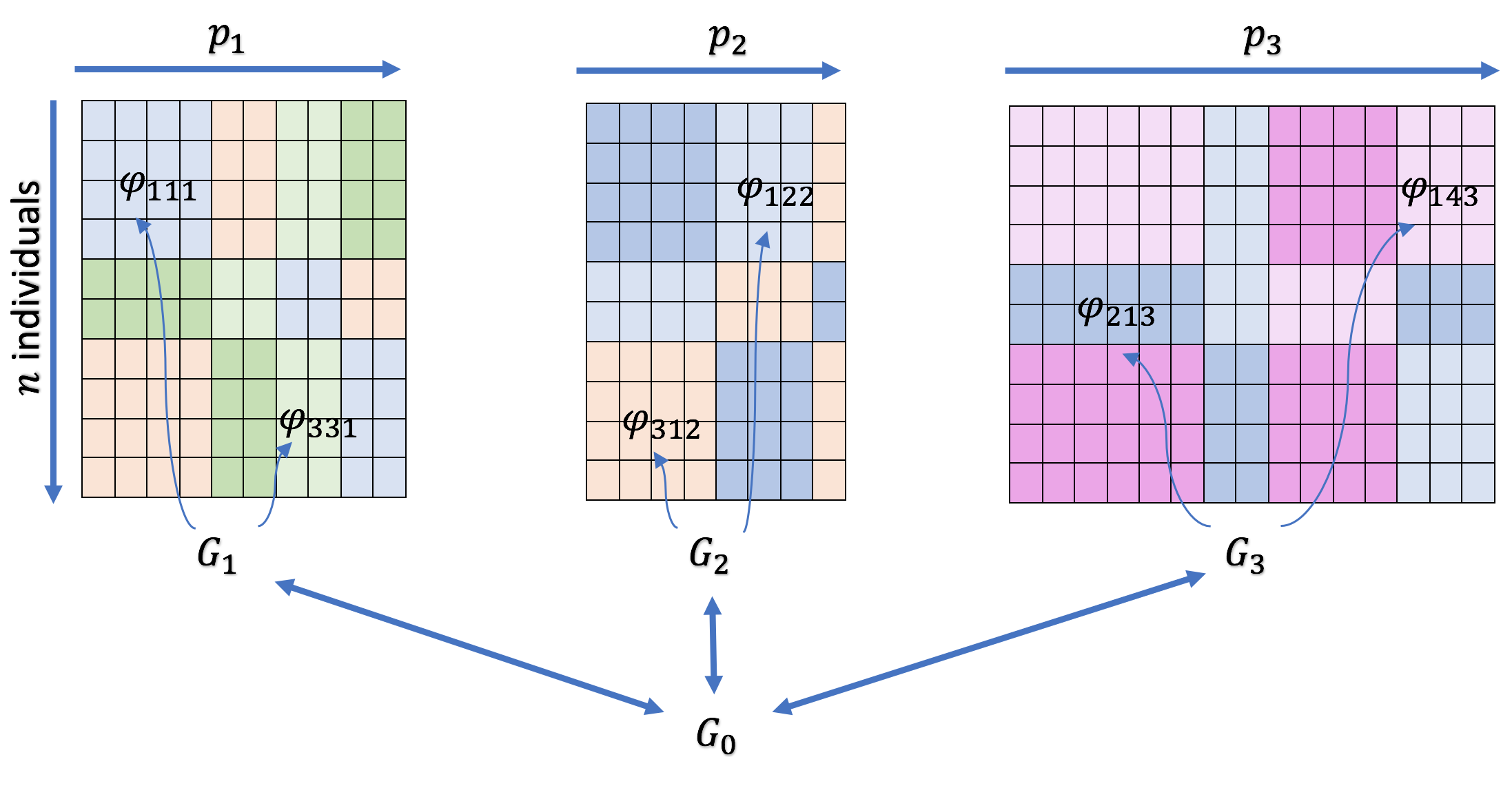
Figure 2: A graphical representation of bidirectional clustering and a hierarchical construction of Dirichlet process. Communications among the various disease subtype–platform combinations is made possible by a higher-level Dirichlet process specification for the base distribution $G_{0}$.

In multiomic datasets, biological information about a disease can be extracted from latent biomarker pathways and patient subpopulations. To capture this aspect of the data, similar to the hierarchical construction of Teh et al. (2006), we model the random base distribution $G_{0}$ of the Dirichlet process prior to allow the bidirectional clusters of the various disease subtype–platform combinations to mutually communicate. This is achieved by a higher-level Dirichlet process specification for base distribution, $G_{0}$, itself: $G_{0}\sim DP\bigl{(}\alpha_{4},N(\mu_{0},\tau_{0}^{2})\bigr{)}$. The discreteness of distribution $G_{0}$ due to the Dirichlet process (Lijoi and Prünster, 2010) is critically important because it causes the atoms of the discrete distributions, $\{G_{t}\}$, to be shared across disease subtype and platform. Consequently, several latent matrix elements of a disease subtype–platform combination are identical to others belonging to a different disease subtype–platform combination. In this manner, we combine unsupervised bidirectional clustering with an effective use of Bayesian mixture models to achieve data integration through sharing of information. See Figure 2 for a graphical representation of the hierarchical structure.

3.2 Models for Survival Outcomes and Gene Selection

We expect only a small fraction of the probes or biomarkers to be associated with the clinical outcome of interest. Extracting the relevant biological features and their relationships with patient outcomes reveals important and possibly unknown biological mechanisms of disease initiation and progression that can be subsequently validated in a wet lab. An important part of effective feature extraction is the elimination of redundancy in the lower-dimensional latent structure detected by the hierarchical model of Section 3.1.

To achieve this, we regard the platform-specific latent clusters as potential predictors and discard repeats in these predictors, so that the number of possible predictors is smaller than the number of total clusters. As mentioned, there are $K_{t}$ column clusters in the $t$th dataset. We aggregate the latent clusters over the $T$ platforms $\bm{Z}_{t}$ by merging clusters that share the same columns of their latent matrices. This reduces the total (across-platform) number of column clusters to $K\leq\sum_{t=1}^{T}K_{t}$. After this merging procedure, let the number of probes associated with the $k$th column cluster be denoted by $N_{k}$, where $k=1,\ldots,K$.

Next, we imagine that each merged column cluster elects from among its member probes a representative, denoted by $\bm{\mu}_{k}$. The column cluster representatives are selected with a priori equal probability from the $N_{k}$ covariates. However, the posterior probabilities of the column cluster representative are usually different for the probes. We rely on an additive regression model that accommodates potential nonlinear functional relationships to detect a typically small subset of the $K$ cluster representatives as the regression predictors. By applying extensions of the spike-and-slab approaches (George and McCulloch, 1993; Karpenko and Dai, 2010; Brown et al., 1998), the additive regression model is $y_{i}\overset{\text{indep}}{\sim}N(\eta_{i},\tau^{2})$, where

$$\eta_{i}=\beta_{0}+\sum_{k=1}^{K}\gamma_{1k}\beta_{1k}\mu_{ik}+\sum_{k=1}^{K}\gamma_{2k}h(\mu_{ik},\beta_{2k}),$$ (1)

$h$ is a nonlinear function and the $\beta$’s are regression coefficients. For an AFT survival outcomes model, we assume $y_{i}=\log(t_{i})$ is a Gaussian regression outcome that is transformed from the uncensored failure time $t_{i}$. As usual, observed survival time $w_{i}=\min\{t_{i},C_{i}\}$ for censoring time $C_{i}$. For column cluster $k$, expression (1) implicitly relies on a triplet of indicators, $\bm{\gamma}_{k}=(\gamma_{0k},\gamma_{1k},\gamma_{2k})$, of which exactly one indicator equals $1$ and the other two indicators equal $0$. For example, if $\gamma_{0k}=1$, then none of the $N_{k}$ probes belonging to column cluster $k$ are associated with the responses. On the other hand, if $\gamma_{1k}=1$, then cluster representative $\bm{\mu}_{k}$ appears as a simple linear regressor. Lastly, if $\gamma_{2k}=1$, then $\bm{\mu}_{k}$ is a nonlinear regressor in (1). The total number of linear predictors, nonlinear predictors, and non-predictors in expression (1) are then $k_{1}=\sum_{k=1}^{K}\gamma_{1k}$, $k_{2}=\sum_{k=1}^{K}\gamma_{2k}$, and $k_{0}=K-k_{1}-k_{2}$, respectively. We collectively denote the $K$ column cluster-specific triplets of indicators by $\bm{\gamma}=(\bm{\gamma}_{1},\cdots,\bm{\gamma}_{K})$.

Due to their interpretability and computational efficiency, one could choose the nonlinear function as order-$s$ splines with $v$ number of knots (De Boor et al., 1978; Hastie and Tibshirani, 1987; Denison et al., 1998). Other options include reproducible kernel Hilbert spaces, nonlinear basis smoothing splines, and wavelets (Mallick et al., 2005; Eubank, 1999). In general, for nonlinear functions $h$ having a linear representation, let $\bm{U}_{\bm{\gamma}}$ be the matrix of $n$ rows consisting of the intercept and $(k_{1}+k_{2})$ regression predictors. Specifically, if we use order-$s$ splines with $v$ number of knots in equation (1), then the number of columns of $\bm{U}_{\bm{\gamma}}$ is $\text{col}(\bm{U}_{\bm{\gamma}})=k_{1}+k_{2}(v+s)+1$.

With $[\cdot]$ denoting densities of random variables, we specify the prior of indicators $\bm{\gamma}$ as $[\bm{\gamma}]\propto\omega^{k_{0}}_{0}\omega^{k_{1}}_{1}\omega^{k_{2}}_{2}\cdot\mathcal{I}\big{(}\text{col}(\bm{U}_{\bm{\gamma}})<n\big{)}$, where probability vector $\bm{\omega}=(\omega_{0},\omega_{1},\omega_{2})$ is given a Dirichlet distribution prior: $\bm{\omega}\sim\mathcal{D}_{3}(1,1,1)$. The truncated prior for $\bm{\gamma}$ ensures model sparsity and prevents overfitting. Finally, conditional on the parameter $\tau^{2}$, we assign a $g$ prior (Zellner, 1986) to the regression coefficients: $\bm{\beta}_{\bm{\gamma}}|\bm{\Sigma}\sim N\big{(}\bm{0},\sigma^{2}_{\beta}\tau^{-2}(\bm{U}_{\bm{\gamma}}^{\prime}\bm{U}_{\bm{\gamma}})^{-1}\big{)}$.

3.3 Posterior Inference

The model parameters are initialized by a naive, separate analysis of each omics platform. Thereafter, the parameters are iteratively updated by MCMC methods. Due to the complex nature of the posterior inference, the procedure is carried out in two stages: (1) platform-specific column cluster and global row cluster detection, followed by (2) predictor discovery for each platform:

1. Stage 1  Focusing only on the multiomic measurements, the column allocation variables, $c_{jt}$, subject–to–row-cluster allocation variables $r_{i}$, and the latent matrix elements $\varphi_{hkt}$, defined in 3.1, are iteratively updated. More specifically:

   • Stage 1a  Using an unrestricted MCMC run, the posterior probability of pairwise clustering of probes are first computed by an MCMC sample. Applying the technique of Dahl (2006), these pairwise probabilities are used to obtain a point estimate for the column cluster allocation variables, $c_{jt}$, for $j=1,\ldots,p_{t}$, $t=1,\ldots,T$, called the column least-squares allocation.

   • Stage 1b  Conditional on the column least-squares allocation, a second MCMC sample is generated. Again using the technique of Dahl (2006), we compute a point estimate, called the row least-squares allocation, for the subject–to–row-cluster allocation variables $r_{1},\ldots,r_{n}$.

   • Stage 1b  Conditional on the bidirectional allocation variables, a third MCMC sample is generated to estimate the latent matrix elements, $\varphi_{hkt}$.

2. Stage 2  Conditional on the column and global row least-squares allocations and latent matrix elements, the patient-specific responses are analyzed using a fourth MCMC sample. In this way, we infer the column cluster predictors and cluster representatives, defined in Section 3.2, and associated with the disease outcomes.

Predictor detection via Bayesian FDR control

When the number of merged clusters $K$ is large, we control the expected Bayesian FDR at nominal level $\alpha$ (Newton et al., 2004; Muller et al., 2006; Morris et al., 2008). Let $b_{k}$ denote the posterior probability that the $k$th merged cluster is a predictor, $k=1,\ldots,K$. Then an MCMC estimate of $b_{k}$ is $\hat{b}_{k}=\frac{1}{M}\sum_{m=1}^{M}\mathcal{I}\bigl{(}\gamma_{1k}^{(m)}+\gamma_{2k}^{(m)}=1\bigr{)}$, where $M$ is the number of MCMC samples. We sort $\hat{b}_{1},\ldots,\hat{b}_{K}$ in descending order to obtain $\hat{b}_{(1)}\geq\ldots\geq\hat{b}_{(K)}$. For a cutoff $\psi_{\alpha}=\hat{b}_{(l)}$, where $l=\max\{k^{*}:\sum_{k=1}^{k^{*}}(1-\hat{b}_{(k)})\leq\alpha\}$. Then the set of merged clusters $\{k:\hat{b}_{k}>\psi_{\alpha}\}$ are declared to be predictive of the clinical outcomes.

4 Results

4.1 Simulation

We investigated the clustering accuracy of the proposed methodology using artificial datasets for which the column clusters and global row clusters are known. No cluster predictors are generated for the responses in this simulation. The data generation procedure consisted of the following two parts:

Probe generation

We generated a dataset consisting of $n=70$ subjects and $T=2$ platforms, with each platform containing $250$ probes, i.e., $p_{1}=p_{2}=250$. Probes for each data are generated from a discrete measure of disease subtype–platform combinations convolved with Gaussian noise, which is further generated from another discrete base distribution. The global row clusters are generated by a finite mixture. We generated the following quantities to obtain transformed data matrix $\bm{Z}_{t}$ of dimension $70\times 250$.

1. True subject–to–row-cluster mappings: Given $n=70$, generate global row clusters labels $\tilde{r}_{1},\cdots,\tilde{r}_{n}$ from a multinomial distribution with equal probabilities $(\frac{1}{3},\frac{1}{3},\frac{1}{3})$. Thus, $\tilde{r}_{i}\in\{1,2,3\}$.

2. True column allocation variables: For platform $t=1,2$, generate $\tilde{c}_{1t},\cdots,\tilde{c}_{p_{t}t}$ as the partitions induced by a PDP with true discount parameters $\tilde{d}_{11}=0.2$ and $\tilde{d}_{12}=0.25$, and with common mass parameter $\tilde{\alpha}_{1}=10$. The true number of clusters, $\tilde{Q}_{t}$, was thereby computed for this non-Dirichlet allocation.

3. True base distribution $\tilde{G}_{0}$: $\tilde{G}_{0}$ is generated from $DP(\tilde{\alpha}_{4},N(\tilde{\mu}_{0},\tilde{\tau}_{0}^{2}))$ according to the stick-breaking process of Sethuraman and Tiwari (1982) and Sethuraman (1994) with $\tilde{\alpha}_{4}=10$, $\tilde{\mu}_{0}=0$, and $\tilde{\tau}_{0}=1$.

4. True discrete measure of disease subtype–platform combinations $\tilde{G}_{1t}$: $\tilde{G}_{1t}$ is generated from $DP(\tilde{\alpha}_{3},\tilde{G}_{0}$) with $\tilde{\alpha}_{3}=10$, again according to a stick-breaking process.

5. Probes for dataset $t$: We generate the latent matrix elements, $\tilde{\varphi}_{hkt}$, as i.i.d samples from $\tilde{G}_{1t}$. The true mapping between $\tilde{\varphi}_{hkt}$ and $Z_{ijt}$ are $\tilde{r}_{1},\cdots,\tilde{r}_{n}$ and $\tilde{c}_{1t},\cdots,\tilde{c}_{p_{t}t}$, and the true noise parameter is $\tilde{\sigma}=0.2$. The elements of a data matrix $\bm{Z}_{t}$ are then distributed as $Z_{ijt}\mid\tilde{r}_{i}=h,\tilde{c}_{jt}=k\overset{indep}{\sim}N(\tilde{\varphi}_{hkt},\tilde{\sigma}^{2})$.

Unsupervised subtypes discovery

Assuming an AFT survival model, apply the procedure as described in Section 3.2 with linear splines and $v=1$ knot per spline. Selecting one probe from each cluster as the representative, variable selection was performed independently for these two data types. Posterior inferences were made according to the stages described in Section 3.3. We evaluate the column clustering and global row clustering accuracy based on the post-processed MCMC samples obtained in Stages 1 and 3 of Section 3.3.

Applying the technique of Dahl (2006) developed for Dirichlet process models, point estimates for the column allocations $\hat{c}_{1t},\cdots,\hat{c}_{p_{t}t}$ are computed. For the full set of probes from the two data types, we estimated the accuracy of the column allocation by the estimated proportion of correctly clustered probe pairs, defined as $\hat{\varkappa}_{t}=\frac{1}{\binom{p_{t}}{2}}\underset{j_{1}\neq j_{2}\in(1,\cdots,p_{t})}{\sum}\mathcal{I}\big{(}\mathcal{I}(\hat{c}_{j_{1}t}=\hat{c}_{j_{2}t})=\mathcal{I}(\tilde{c}_{j_{1}t}=\tilde{c}_{j_{2}t})\big{)}$.

Also applying the technique of Dahl (2006), point estimates for subject–to–row-cluster mappings $\hat{r}_{1},\cdots,\hat{r}_{n}$ were computed. We estimated the accuracy of subject–to–row-cluster mappings in the same way: $\hat{\vartheta}=\frac{1}{\binom{n}{2}}\underset{i_{1}\neq i_{2}\in(1,\cdots,n)}{\sum}\mathcal{I}\big{(}\mathcal{I}(\hat{r}_{i_{1}}=\hat{r}_{i_{2}})=\mathcal{I}(\tilde{r}_{i_{1}}=\tilde{r}_{i_{2}})\big{)}$. High values of $\hat{\varkappa}_{t}$ and $\hat{\vartheta}$ are indicative of high clustering accuracy for all $p_{t}$ probes and all $n$ subjects.

Table 1 displays the mean percentages $\hat{\varkappa}_{t}$ and estimated $R^{2}$ averaged over $50$ independent replications. The mean proportion of correctly clustered subject pairs $\hat{\vartheta}$ is 0.955 (0.042), with standard error shown in parentheses. We find that significantly less than 5% pairs of subjects are incorrectly clustered in the same global row clusters out of $\binom{70}{2}=2415$ different subjects pairs, and significantly less than 3% pairs of probes are incorrectly clustered among $\binom{250}{2}=31125$ different probe pairs in each platform. Thus, over $50$ replication, we observed highly accurate clustering-related inferences for the global row clusters as well as for the full set of $p=250$ probes of every platform. The high accuracy is also reflected by the estimated $R^{2}$’s, all of which are significantly greater than $90\%$.

To further demonstrate the performance of our method, we generated $12$ setups, with $T=2$ data types. We generated $h=3,4,5$ global row clusters using the same way as the previous simulation in Section 4.1. For each value of $h$, we varied the data noise $\tilde{\sigma}$ among $0.2,0.3,0.4,0.5$. For each set up, we replicated the procedure $50$ times. Therefore, we covered situations ranging from few global row clusters with small noise to many global row clusters with large noise.

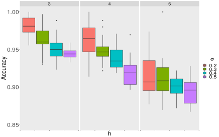
Figure 3: Side-by-side boxplots comparing combination of different numbers of global row clusters and $\sigma$ values.

The subject–to–row-cluster mappings accuracy is consistently going up as $h$ reaches 5 as shown in Figure 3. It moderately goes down as more noise involved; however, it remains above $90\%$ when global row clusters is $5$.

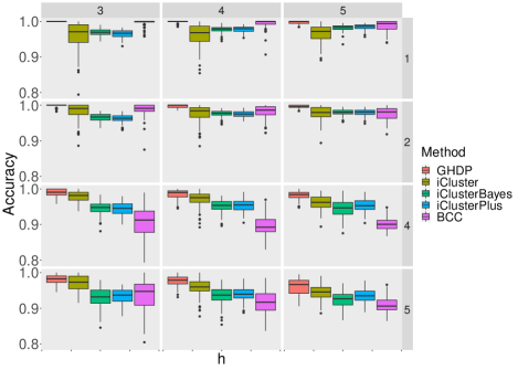
Figure 4: Side-by-side boxplots comparing the proposed method with iCluster, iClusterBayes, iClusterPlus, and BCC over $12$ combinations of different numbers of global row clusters and noise levels.

Furthermore, we evaluated our model’s performance in subject–to–row-cluster mappings by comparing it with other model-based integrative clustering methods. These methods include iCluster, iClusterPlus, iClusterBayes (Shen et al., 2009; Mo et al., 2013, 2018), and Bayesian consensus clustering (BCC) (Lock and Dunson, 2013). For a fair comparison, we simulated data as a mixture of multivariate Gaussians with non-trivial correlation structure and varying noise levels using the MixSim R-package (Melnykov et al., 2012). In specific, the package is used to simulate $h=3,4,5$ cluster-specific mean vectors, $p_{t}\times p_{t}$ cluster specific full covariance matrices for $p_{t}=250$, $t=1,2$, and with different noise levels. We repeated the simulation settings $100$ times and compared the results with other competing methods. For BCC, we assume that the data sources are equally adhering to the overall clustering, and specify the true number of global row clusters as the number of overall clustering. Figure 4 depicts boxplots of the estimated proportion of correctly clustered subject pairs for our method and others. Our method remains above $95\%$ subject–to–row-cluster allocation accuracy for all $12$ set ups, with considerably smaller standard errors in most set ups.

4.2 An application to TCGA datasets

The proposed methodology is applied to a lung cancer dataset available from TCGA. TCGA includes tumor samples from more than $500$ patients with lung cancer. Analyzing different platforms illuminates some of the biomolecular characteristics in lung cancer. For example, the iCluster methods (Mo et al., 2018, 2013; Shen et al., 2009) developed a joint latent variable model for integrative clustering of copy number and gene expression data. Kim et al. (2015) introduced an integrative phenotyping framework (iPF) for disease subtype discovery. LUSC and LUAD are two main subtypes of lung cancer. They are the most common type of NSCLC, and LUAD has a high rate of mutations compared to other cancers. Previous studies regarding molecular profiling of LUSC and LUAD have been extensively discussed (Carrot-Zhang et al., 2020; Cancer Genome Atlas Research Network, 2014, 2012). Four subtypes of LUSC were molecularly described, classical, basal, secretory, and primitive. Three distinct molecular subtypes of LUAD have been discovered based on gene expression data, proximal inflammatory (PI), proximal proliferative (PP), and terminal respiratory unit (TRU). These subtypes were observed to be relevant to pathways and clinical outcomes and may offer insight into targeted therapies.

Here, we concentrate on integrating gene expression and DNA methylation data. We downloaded the data from the TCGA website: https://cancergenome.nih.gov/ (see also International Cancer Genome Consortium, 2010) using the TCGA assembler 2 R package (Wei et al., 2017; Zhu et al., 2014). The gene expression profile is obtained using Illumina HiSeq Array, and the data were normalized counts of genes. The DNA methylation data, which contains percentage of methylation, is obtained using the Infinium Human Methylation 450 BeadChip. We acquired the level $3$ data for gene expression and DNA methlyation. We now briefly summarize the data pre-processing steps for both data as follows. We first filter out those genes with less than $5\%$ somatic mutation. Then we filter out the under-expressed genes with mean of normalized expression less than $3.5$, and standard deviation less than $1.7$. For the methylation data, we filter out the features for which the standard deviation of the percentages is less than $0.01$. Finally, clinical data is matched with samples that have both gene expression and DNA methylation data. After these steps, a common set of $88$ tumor samples is obtained, and the platforms consist of RNA gene expression data for $309$ genes and DNA methylation data for $288$ features.

We applied the model described in Section 3.1 and the MCMC procedure detailed in Section 3.3 to obtain a global row clustering of patients with allowing platform-specific column clustering of probes, then to select informative cluster predictors by applying the variable selection procedure described in Section 3.2.

Identification of cancer subtypes

A point estimate of global row clusters were obtained via Dahl (2006) to ease visualization and interpretation. Table 2 and 3 respectively show matching matrices comparing the global row clusters given by our method with the cancer subtypes and transcriptional subtypes defined by TCGA.

Our method discovered different clustering structures than the subtypes defined by TCGA, but not independent (Fisher’s exact test, p-value $\ll 0.0001$). Clusters $1$, $2$ and $3$ primarily represent finer subpopulations of the LUAD samples which usually have a high rate of mutations. Cluster 1 corresponds to the transcriptional subtype proximal-inflammatory (PI), which was featured by co-mutation of tumour suppressor genes NF1 and TP53 as described in Cancer Genome Atlas Research Network (2014). Cluster 2 and 3 are primarily subsets of proximal-proliferative (PP) that was enriched for mutation of KRAS. To examine chromatin states as suggested by Cancer Genome Atlas Research Network (2014), a measure of methylation level at CpG island methylator phenotype (CIMP) sites is used. Majority proportions of cluster 1 and 2 ($75\%$ and $60\%$ respectively) correspond to DNA hypermethylation. Cluster 3 links to a more normal-like CIMP-low group (73%). The prognosis for lung cancer is poor, our method reveals a well separation between samples that have different prognosis. Cluster 3 is formed by the samples with the worst 3-year survival rate of $0.08\pm 0.07$, whereas cluster 4, mainly consists of the LUSC samples, has significantly better prognosis in 3 years, but with 6-year survival rate only $0.14\pm 0.09$. The Kaplan-Meier survival curves for all global row clusters show significant difference (log-rank test p-value $\ll 0.0001$).

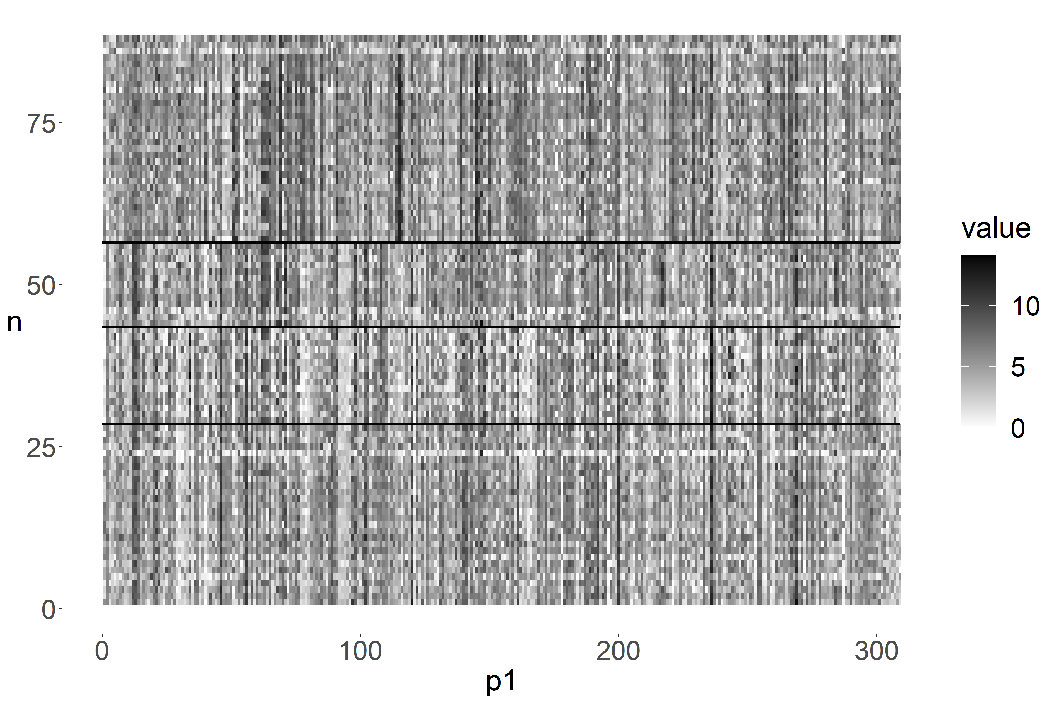
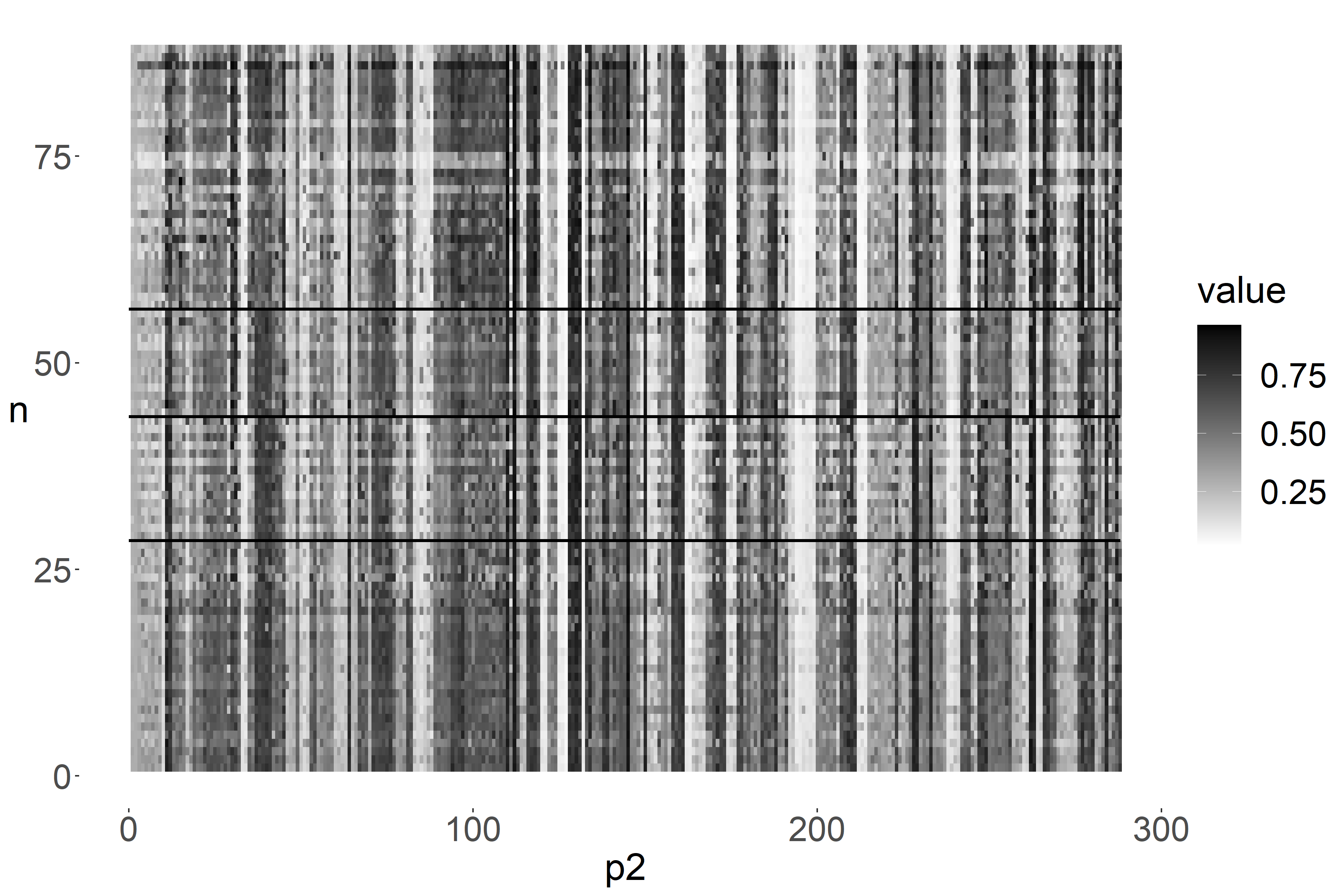
Figure 5: Heatmaps of gene expression (mRNA) and DNA methylation. Samples are arranged by both row least-squares allocation and column least-squares allocation under the proposed model.

Figure 5 shows the heatmap of mRNA and methylation with samples rearranged by their row least-squares allocation and probes rearranged by column least-squares allocation. The cluster are annotated in a descending order. We annotate the cluster at the bottom of each heatmap as cluster $1$, the cluster at the top of each heatmap as cluster $4$.

Selected features

Applying the gene selection technique described in Section 3.2, and at Bayesian FDR = $0.2$, $64$ among the $239$ column clusters discovered in mRNA are selected as cluster predictors. Whereas, $14$ among $79$ column clusters discovered in methylation are selected as cluster predictors. Among the $78$ cluster predictors detected from either mRNA or methylation platform, we list the top eight clusters that are most predictive of patients’ survival outcomes in Table 4, with the posterior probabilities of being selected as predictors greater than 0.8. Since the cluster labels are arbitrary, we rank them in descending order of the posterior probabilities, with cluster $1$ as the most predictive. Each cluster contains one or multiple genes or CpG islands along with their posterior probabilities of being selected as a cluster representative, e.g., gene ORM1 has a posterior probability of $0.217$ of being the cluster representative of cluster $4$.

These results confirm several findings in the scientific literature. Relli et al. (2018) discovered tumor prognostic drivers that have impact on LUSC or LUAD clinical outcome based on a next generation sequencing analysis of the NSCLC. Among the discovered determinants, SERPINB5 overexpression is related to dismal prognosis in LUAD. As the RNA level analysis in this paper extended to protein level, the protein coded by FGFBP1 gene is one of the key proteomic signatures in the prognosis profiles of either lung cancer subtype. Jiang et al. (2016) suggested several SNPs at the TOX3/LOC643714 locus that might promote lung cancer risk. The locus was previously identified through GWAS as one of the first regions associated with breast cancer. Recently, Bauer et al. (2017) discovered that lung tumor promotion was significantly reduced in the EREG knockout compared to wildtype controls in a murine model, suggesting that EREG could be used as a biomarker as well as a potential novel target in lung cancer, which largely overlaps with our findings. Another study aimed to understand the mechanisms behind epidermal growth factor receptor tyrosine kinase inhibitors (EGFR-TKIs) resistance further suggested that EREG, predominantly produced in macrophages in the tumor tissue, as a novel biomarker and moderator for EGFR-TKI therapeutics (Ma et al., 2021).

5 Discussion

In this article, we have proposed an innovative, flexible and scalable Bayesian nonparametric framework for analyzing multi-domain array and next generation sequencing-based omics datasets, and detecting various aspects of molecular drivers for multiple platforms. Different from most model based integrative analysis, which focus on either identifying biological associations of probes among different platforms or grouping subjects according to the similarities of their molecular entities, our model involves a nonparametric hierarchical structure, which estimates biological mechanisms by an effective bidirectional clustering to achieve dimension reduction at both probes and subjects level. Additionally, an efficient variable selection procedure is implemented to identify relevant biological features that can potentially reveal underlying drivers of a disease.

The major task of the model is to identify cancer subtypes. Through simulation studies and comparisons, our model gives high clustering accuracy in global subject–to–row-cluster mappings and data platforms specific local column allocation of features. The application to TCGA data confirms the molecular profiling of LUSC and LUAD discussed in previous literature that may offer perception into targeted therapies. The proposed model provides an intuitive and insightful setting for integrative clustering of multiple domains to improve cancer subtype diagnosis and prognosis.

Even though the motivating data involves two platforms, the methodology proposed in this paper can be applied as is to an arbitrary number of platforms and disease subtypes. Generalization to count, categorical, and ordinal probes is possible. It is important to investigate the dependence structures and theoretical properties associated with the more general framework. This will be the focus of our group’s future research.

As a result of the complex nature of the MCMC inference, we performed these analyses in two stages, with bidirectional clustering followed by subtypes discovery, then predictor discovery. We are currently working on implementing the MCMC procedure in a parallel computing structure using graphical processing units (GPU) (Suchard et al., 2010). We plan to make the software available as an R package for general use in the near future.

Table 1: Column 2 displays the mean proportion of correctly clustered probe pairs. Column 3 displays the estimated $R^{2}$, with the standard errors for the $50$ independent replications shown in parentheses.

		Percent $\hat{\varkappa}_{1t}$	Estimated $R^{2}$
	$t=1$	0.971 (0.010)	0.924 (0.038)
	$t=2$	0.975 (0.011)	0.943 (0.025)

Table 2: Global row clustering versus TCGA comprehensive subtype matching matrix

	Row cluster
Cancer subtypes	1	2	3	4
LUAD	28	15	11	2
LUSC	0	0	2	30
3-year survival	$0.36\pm 0.09$	$0.40\pm 0.12$	$0.08\pm 0.07$	$0.63\pm 0.08$

Table 3: First three global row clusters versus TCGA lung adenocarcinoma (LUAD) molecular subtypes matching matrix

	Row cluster
Molecular subtypes of LUAD	1	2	3
Proximal-inflammatory (PI)	23	1	2
Proximal-proliferative (PP)	0	9	8
Terminal respiratory unit (TRU)	5	5	1
Mutation rate
NF1	32%	13%	9%
TP53	75%	26%	36%
KRAS	17%	33%	36%
Methylation level
CIMP-high	11%	40%	18%
CIMP-intermediate	64%	20%	9%

Table 4: Top eight clusters of mRNA and methylation that are most predictive

Cluster	Platform	Gene or CpG island	Probability
1	mRNA	FGFBP1	1
2	mRNA	SERPINB5	1
3	mRNA	TOX3	1
		ORM1	0.217
		VSIG2	0.213
4	mRNA	SFTA1P	0.185
		PLA2G10	0.156
		CFAP221	0.131
		COL4A3	0.099
5	mRNA	EREG	1
		SFRP1	0.150
		FOXA2	0.130
		TOX3	0.115
		PEG10	0.111
6	Methylation	CFAP221	0.110
		GFRA3	0.109
		KREMEN2	0.095
		NSG1	0.095
		CRYM	0.087
		CNTN1	0.368
7	mRNA	VSNL1	0.353
		GRHL3	0.279
		SAA2	0.362
8	Methylation	CYP4B1	0.356
		MUC13	0.283

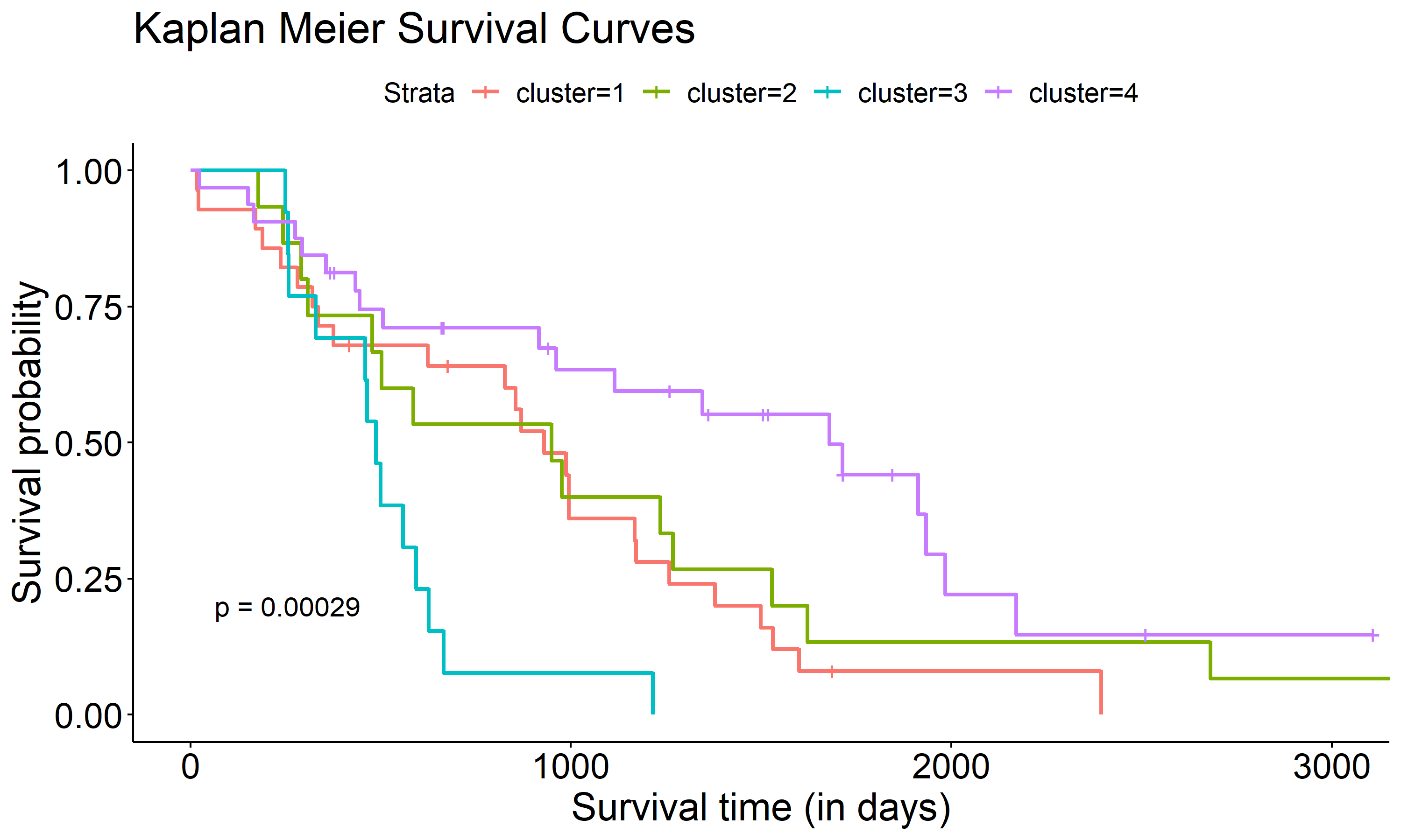
Figure 6: Kaplan-Meier survival curves of discovered global row clusters for lung cancer specific survivals. Crosses indicate censored outcomes.

References

- Ahmad and Fröhlich (2017) Ahmad, A. and Fröhlich, H. (2017). Towards clinically more relevant dissection of patient heterogeneity via survival-based bayesian clustering. Bioinformatics, 33(22), 3558–3566.
- Bauer et al. (2017) Bauer, A. K., Velmurugan, K., Xiong, K.-N., Alexander, C.-M., Xiong, J., and Brooks, R. (2017). Epiregulin is required for lung tumor promotion in a murine two-stage carcinogenesis model. Molecular carcinogenesis, 56(1), 94–105.
- Brown et al. (1998) Brown, P. J., Vannucci, M., and Fearn, T. (1998). Multivariate bayesian variable selection and prediction. Journal of the Royal Statistical Society: Series B (Statistical Methodology), 60(3), 627–641.
- Cancer Genome Atlas Research Network (2012) Cancer Genome Atlas Research Network (2012). Comprehensive genomic characterization of squamous cell lung cancers. Nature, 489(7417), 519.
- Cancer Genome Atlas Research Network (2014) Cancer Genome Atlas Research Network (2014). Comprehensive molecular profiling of lung adenocarcinoma. Nature, 511(7511), 543–550.
- Carrot-Zhang et al. (2020) Carrot-Zhang, J., Chambwe, N., Damrauer, J. S., Knijnenburg, T. A., Robertson, A. G., Yau, C., Zhou, W., Berger, A. C., Huang, K.-l., Newberg, J. Y., et al. (2020). Comprehensive analysis of genetic ancestry and its molecular correlates in cancer. Cancer Cell, 37(5), 639–654.
- Cenik et al. (2015) Cenik, C., Cenik, E. S., Byeon, G. W., Grubert, F., Candille, S. I., Spacek, D., Alsallakh, B., Tilgner, H., Araya, C. L., Tang, H., et al. (2015). Integrative analysis of rna, translation, and protein levels reveals distinct regulatory variation across humans. Genome research, 25(11), 1610–1621.
- Choi et al. (2017) Choi, W., Ochoa, A., McConkey, D. J., Aine, M., Höglund, M., Kim, W. Y., Real, F. X., Kiltie, A. E., Milsom, I., Dyrskjøt, L., et al. (2017). Genetic alterations in the molecular subtypes of bladder cancer: illustration in the cancer genome atlas dataset. European urology, 72(3), 354–365.
- Coretto et al. (2018) Coretto, P., Serra, A., and Tagliaferri, R. (2018). Robust clustering of noisy high-dimensional gene expression data for patients subtyping. Bioinformatics, 34(23), 4064–4072.
- Dahl (2006) Dahl, D. B. (2006). Model-based clustering for expression data via a dirichlet process mixture model. Bayesian inference for gene expression and proteomics, 201, 218.
- De Boor et al. (1978) De Boor, C., De Boor, C., Mathématicien, E.-U., De Boor, C., and De Boor, C. (1978). A practical guide to splines, volume 27. Springer-Verlag New York.
- Denison et al. (1998) Denison, D., Mallick, B., and Smith, A. (1998). Automatic bayesian curve fitting. Journal of the Royal Statistical Society: Series B (Statistical Methodology), 60(2), 333–350.
- Dunson and Park (2008) Dunson, D. B. and Park, J.-H. (2008). Kernel stick-breaking processes. Biometrika, 95(2), 307–323.
- Dunson et al. (2008) Dunson, D. B., Herring, A. H., and Engel, S. M. (2008). Bayesian selection and clustering of polymorphisms in functionally related genes. Journal of the American Statistical Association, 103(482), 534–546.
- Eubank (1999) Eubank, R. L. (1999). Nonparametric regression and spline smoothing. CRC press.
- Fan et al. (2019) Fan, S., Tang, J., Li, N., Zhao, Y., Ai, R., Zhang, K., Wang, M., Du, W., and Wang, W. (2019). Integrative analysis with expanded dna methylation data reveals common key regulators and pathways in cancers. NPJ genomic medicine, 4(1), 1–11.
- George and McCulloch (1993) George, E. I. and McCulloch, R. E. (1993). Variable selection via gibbs sampling. Journal of the American Statistical Association, 88(423), 881–889.
- Guha (2010) Guha, S. (2010). Posterior simulation in countable mixture models for large datasets. Journal of the American Statistical Association, 105(490), 775–786.
- Guha and Baladandayuthapani (2016) Guha, S. and Baladandayuthapani, V. (2016). A nonparametric bayesian technique for high-dimensional regression. Electronic Journal of Statistics, 10(2), 3374–3424.
- Haakensen et al. (2016) Haakensen, V. D., Nygaard, V., Greger, L., Aure, M. R., Fromm, B., Bukholm, I. R., Lüders, T., Chin, S.-F., Git, A., Caldas, C., et al. (2016). Subtype-specific micro-rna expression signatures in breast cancer progression. International journal of cancer, 139(5), 1117–1128.
- Hastie and Tibshirani (1987) Hastie, T. and Tibshirani, R. (1987). Generalized additive models: some applications. Journal of the American Statistical Association, 82(398), 371–386.
- International Cancer Genome Consortium (2010) International Cancer Genome Consortium (2010). International network of cancer genome projects. Nature, 464(7291), 993.
- Jiang et al. (2016) Jiang, C., Yu, S., Qian, P., Guo, R., Zhang, R., Ao, Z., Li, Q., Wu, G., Chen, Y., Li, J., et al. (2016). The breast cancer susceptibility-related polymorphisms at the tox3/loc643714 locus associated with lung cancer risk in a han chinese population. Oncotarget, 7(37), 59742.
- Karpenko and Dai (2010) Karpenko, O. and Dai, Y. (2010). Relational database index choices for genome annotation data. In Bioinformatics and Biomedicine Workshops (BIBMW), 2010 IEEE International Conference on, pages 264–268. IEEE.
- Kim et al. (2006) Kim, S., Tadesse, M. G., and Vannucci, M. (2006). Variable selection in clustering via dirichlet process mixture models. Biometrika, 93(4), 877–893.
- Kim et al. (2015) Kim, S., Herazo-Maya, J. D., Kang, D. D., Juan-Guardela, B. M., Tedrow, J., Martinez, F. J., Sciurba, F. C., Tseng, G. C., and Kaminski, N. (2015). Integrative phenotyping framework (ipf): integrative clustering of multiple omics data identifies novel lung disease subphenotypes. BMC genomics, 16(1), 924.
- Lian et al. (2019) Lian, H., Han, Y.-P., Zhang, Y.-C., Zhao, Y., Yan, S., Li, Q.-F., Wang, B.-C., Wang, J.-J., Meng, W., Yang, J., et al. (2019). Integrative analysis of gene expression and dna methylation through one-class logistic regression machine learning identifies stemness features in medulloblastoma. Molecular oncology, 13(10), 2227–2245.
- Lijoi and Prünster (2010) Lijoi, A. and Prünster, I. (2010). Models beyond the dirichlet process. Bayesian nonparametrics, 28(80), 3.
- Lijoi et al. (2007) Lijoi, A., Mena, R. H., and Prünster, I. (2007). Bayesian nonparametric estimation of the probability of discovering new species. Biometrika, 94(4), 769–786.
- Lock and Dunson (2013) Lock, E. F. and Dunson, D. B. (2013). Bayesian consensus clustering. Bioinformatics, 29(20), 2610–2616.
- Ma et al. (2021) Ma, S., Zhang, L., Ren, Y., Dai, W., Chen, T., Luo, L., Zeng, J., Mi, K., Lang, J., and Cao, B. (2021). Epiregulin confers egfr-tki resistance via egfr/erbb2 heterodimer in non-small cell lung cancer. Oncogene, 40(14), 2596–2609.
- Maity et al. (2020) Maity, A. K., Lee, S. C., Mallick, B. K., and Sarkar, T. R. (2020). Bayesian structural equation modeling in multiple omics data with application to circadian genes. Bioinformatics, 36(13), 3951–3958.
- Mallick et al. (2005) Mallick, B. K., Ghosh, D., and Ghosh, M. (2005). Bayesian classification of tumours by using gene expression data. Journal of the Royal Statistical Society: Series B (Statistical Methodology), 67(2), 219–234.
- Medvedovic et al. (2004) Medvedovic, M., Yeung, K. Y., and Bumgarner, R. E. (2004). Bayesian mixture model based clustering of replicated microarray data. Bioinformatics, 20(8), 1222–1232.
- Melnykov et al. (2012) Melnykov, V., Chen, W.-C., and Maitra, R. (2012). Mixsim: An r package for simulating data to study performance of clustering algorithms. Journal of Statistical Software, 51(12), 1.
- Mo et al. (2013) Mo, Q., Wang, S., Seshan, V. E., Olshen, A. B., Schultz, N., Sander, C., Powers, R. S., Ladanyi, M., and Shen, R. (2013). Pattern discovery and cancer gene identification in integrated cancer genomic data. Proceedings of the National Academy of Sciences, 110(11), 4245–4250.
- Mo et al. (2018) Mo, Q., Shen, R., Guo, C., Vannucci, M., Chan, K. S., and Hilsenbeck, S. G. (2018). A fully bayesian latent variable model for integrative clustering analysis of multi-type omics data. Biostatistics, 19(1), 71–86.
- Morris et al. (2008) Morris, J. S., Brown, P. J., Herrick, R. C., Baggerly, K. A., and Coombes, K. R. (2008). Bayesian analysis of mass spectrometry proteomic data using wavelet-based functional mixed models. Biometrics, 64(2), 479–489.
- Muller et al. (2006) Muller, P., Parmigiani, G., and Rice, K. (2006). Fdr and bayesian multiple comparisons rules.
- Navin (2014) Navin, N. E. (2014). Cancer genomics: one cell at a time. Genome biology, 15(8), 1–13.
- Newton et al. (2004) Newton, M. A., Noueiry, A., Sarkar, D., and Ahlquist, P. (2004). Detecting differential gene expression with a semiparametric hierarchical mixture method. Biostatistics, 5(2), 155–176.
- Park et al. (2021) Park, S., Xu, H., and Zhao, H. (2021). Integrating multidimensional data for clustering analysis with applications to cancer patient data. Journal of the American Statistical Association, 116(533), 14–26.
- Perman et al. (1992) Perman, M., Pitman, J., and Yor, M. (1992). Size-biased sampling of poisson point processes and excursions. Probability Theory and Related Fields, 92(1), 21–39.
- Pitman (1995) Pitman, J. (1995). Exchangeable and partially exchangeable random partitions. Probability theory and related fields, 102(2), 145–158.
- Pitman and Yor (1997) Pitman, J. and Yor, M. (1997). The two-parameter poisson-dirichlet distribution derived from a stable subordinator. The Annals of Probability, pages 855–900.
- Relli et al. (2018) Relli, V., Trerotola, M., Guerra, E., and Alberti, S. (2018). Distinct lung cancer subtypes associate to distinct drivers of tumor progression. Oncotarget, 9(85), 35528.
- Sethuraman (1994) Sethuraman, J. (1994). A constructive definition of dirichlet priors. Statistica sinica, pages 639–650.
- Sethuraman and Tiwari (1982) Sethuraman, J. and Tiwari, R. C. (1982). Convergence of dirichlet measures and the interpretation of their parameter. In Statistical decision theory and related topics III, pages 305–315. Elsevier.
- Shen et al. (2009) Shen, R., Olshen, A. B., and Ladanyi, M. (2009). Integrative clustering of multiple genomic data types using a joint latent variable model with application to breast and lung cancer subtype analysis. Bioinformatics, 25(22), 2906–2912.
- Simon and Roychowdhury (2013) Simon, R. and Roychowdhury, S. (2013). Implementing personalized cancer genomics in clinical trials. Nature reviews Drug discovery, 12(5), 358–369.
- Singh et al. (2019) Singh, A., Shannon, C. P., Gautier, B., Rohart, F., Vacher, M., Tebbutt, S. J., and Lê Cao, K.-A. (2019). Diablo: an integrative approach for identifying key molecular drivers from multi-omics assays. Bioinformatics, 35(17), 3055–3062.
- Singh et al. (2020) Singh, N., Mishra, A., Sahu, D. K., Jain, M., Shyam, H., Tripathi, R. K., Shankar, P., Kumar, A., Alam, N., Jaiswal, R., et al. (2020). Comprehensive characterization of stage iiia non-small cell lung carcinoma. Cancer Management and Research, 12, 11973.
- Suchard et al. (2010) Suchard, M. A., Wang, Q., Chan, C., Frelinger, J., Cron, A., and West, M. (2010). Understanding gpu programming for statistical computation: Studies in massively parallel massive mixtures. Journal of computational and graphical statistics, 19(2), 419–438.
- Teh et al. (2006) Teh, Y. W., Jordan, M. I., Beal, M. J., and Blei, D. M. (2006). Hierarchical dirichlet processes. Journal of the American Statistical Association, 101, 1566–1581.
- Wang et al. (2018) Wang, D., Li, J.-R., Zhang, Y.-H., Chen, L., Huang, T., and Cai, Y.-D. (2018). Identification of differentially expressed genes between original breast cancer and xenograft using machine learning algorithms. Genes, 9(3), 155.
- Wang et al. (2013) Wang, W., Baladandayuthapani, V., Morris, J. S., Broom, B. M., Manyam, G., and Do, K.-A. (2013). ibag: integrative bayesian analysis of high-dimensional multiplatform genomics data. Bioinformatics, 29(2), 149–159.
- Wei et al. (2017) Wei, L., Jin, Z., Yang, S., Xu, Y., Zhu, Y., and Ji, Y. (2017). Tcga-assembler 2: software pipeline for retrieval and processing of tcga/cptac data. Bioinformatics, 34(9), 1615–1617.
- Wu et al. (2018) Wu, Y., Zeng, J., Zhang, F., Zhu, Z., Qi, T., Zheng, Z., Lloyd-Jones, L. R., Marioni, R. E., Martin, N. G., Montgomery, G. W., et al. (2018). Integrative analysis of omics summary data reveals putative mechanisms underlying complex traits. Nature communications, 9(1), 1–14.
- Yang et al. (2017) Yang, H., Wei, Q., Zhong, X., Yang, H., and Li, B. (2017). Cancer driver gene discovery through an integrative genomics approach in a non-parametric bayesian framework. Bioinformatics, 33(4), 483–490.
- Yoo et al. (2019) Yoo, S.-K., Song, Y. S., Lee, E. K., Hwang, J., Kim, H. H., Jung, G., Kim, Y. A., Kim, S.-j., Cho, S. W., Won, J.-K., et al. (2019). Integrative analysis of genomic and transcriptomic characteristics associated with progression of aggressive thyroid cancer. Nature communications, 10(1), 1–12.
- Zellner (1986) Zellner, A. (1986). On assessing prior distributions and bayesian regression analysis with g-prior distributions. Bayesian inference and decision techniques.
- Zhu et al. (2014) Zhu, Y., Qiu, P., and Ji, Y. (2014). Tcga-assembler: open-source software for retrieving and processing tcga data. Nature methods, 11(6), 599.