Unsupervised Time-Series Representation Learning with
Iterative Bilinear Temporal-Spectral Fusion

Abstract

Unsupervised/self-supervised time series representation learning is a challenging problem because of its complex dynamics and sparse annotations. Existing works mainly adopt the framework of contrastive learning with the time-based augmentation techniques to sample positives and negatives for contrastive training. Nevertheless, they mostly use segment-level augmentation derived from time slicing, which may bring about sampling bias and incorrect optimization with false negatives due to the loss of global context. Besides, they all pay no attention to incorporate the spectral information in feature representation. In this paper, we propose a unified framework, namely Bilinear Temporal-Spectral Fusion (BTSF). Specifically, we firstly utilize the instance-level augmentation with a simple dropout on the entire time series for maximally capturing long-term dependencies. We devise a novel iterative bilinear temporal-spectral fusion to explicitly encode the affinities of abundant time-frequency pairs, and iteratively refines representations in a fusion-and-squeeze manner with Spectrum-to-Time (S2T) and Time-to-Spectrum (T2S) Aggregation modules. We firstly conducts downstream evaluations on three major tasks for time series including classification, forecasting and anomaly detection. Experimental results shows that our BTSF consistently significantly outperforms the state-of-the-art methods.

1 Introduction

Time series analysis (Oreshkin et al., 2020) plays a crucial role in various real-world scenarios, such as traffic

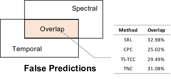
Figure 1: Statistics about false predictions of randomly selected evaluation samples.

prediction, clinical trials and financial market. Classification (Esling & Agon, 2012), forecasting (Deb et al., 2017) and anomaly detection (Laptev et al., 2015) are main tasks for time series analysis. However, there is often no adequate labeled data for training and results are not ideal when time series are sparsely labeled or without supervision (Lan et al., 2021). Therefore, it is valuable to study on the unsupervised representation learning for time series with which the learned representations can be used for aforementioned downstream tasks. Unsupervised representation learning has been well studied in computer vision and natural language processing (Denton & Birodkar, 2017; Gutmann & Hyvärinen, 2012; Wang & Gupta, 2015; Pagliardini et al., 2018; Chen et al., 2020b) but only a few researches are related with time series analysis (Eldele et al., 2021b; Yue et al., 2021b; Liu et al., 2021).

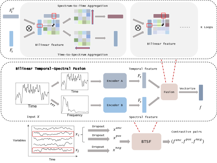
Figure 2: The diagram of our general unsupervised representation learning framework for multivariate time series, $\otimes$ is the cross product. See Section 3.2 for more details.

Recent works mainly utilize the time-based contrastive learning framework (Chen et al., 2020a; Zerveas et al., 2021) for unsupervised representation learning in time series. Time-Contrastive Learning (TCL) (Hyvarinen & Morioka, 2016), Contrastive Predictive Coding (CPC) (Oord et al., 2018), Scalable RepresentationLearning (SRL) (Franceschi et al., 2019), Temporal and Contextual Contrasting (TS-TCC) (Eldele et al., 2021b) and Temporal Neighborhood Coding(TNC) (Tonekaboni et al., 2021) are all segment-level methods which sample contrastive pairs along temporal axis. Nevertheless, they all fail to utilize the temporal-spectral affinities in time series and thus limit the discriminativity and expressiveness of the representations. We further take an experimental analysis on these methods and Figure 1 shows statistics about false predictions on time series classification. We implement existing works according to public codes. In specific, by spectral means we use their proposed sampling methods to generate contrastive pairs and transform the sampled time series into spectral domain for extracting feature for later training and testing. It is notable that existing works all have a low overlap percentage around 30% about false predictions with only temporal or spectral feature. The phenomenon demonstrates their temporal and spectral representations have few associations. Besides, previous segment-level methods are based on the assumption that distant segments are negative pairs and neighbour segments are positive pairs, which usually perform badly in long-term scenarios and fail to capture the global context.

Based on the aforementioned shortcomings of existing works, we propose an unsupervised representation learning framework for time series, namely Bilinear Temporal-Spectral Fusion (BTSF). BTSF promotes the representation learning process from two aspects, the more reasonable construction of contrastive pairs and the adequate integration of temporal and spectral information. In order to preserve the global temporal information and have the ability to capture long-term dependencies of time series, BTSF uses the entire time series as input and simply applies a standard dropout (Srivastava et al., 2014) as an instance-level augmentation to produce different views of time series. Such construction of contrastive pairs ensures that the augmented time series would not change their raw properties, which effectively reduces the possible false negatives and positives. For the effective combination of temporal-spectral information and further achieving alignment between them in feature representation, we perform an iterative bilinear fusion between temporal and spectral features to produce a fine-grained second-order feature which explicitly preserves abundant pairwise temporal-spectral affinities. To adequately utilize the informative affinities, we further design a cross-domain interaction with Spectrum-to-Time and Time-to-Spectrum Aggregation modules to iteratively refine temporal and spectral features for cycle update. Compared to simple combination operations like summation and concatenation, our bilinear fusion make it possible that the temporal (spectral) feature gets straightly enhanced by spectral (temporal) information of the same time series, which is proved to be effective by our further experiments and theoretical analysis.

Our main contributions are summarized as the following:

• We revisit the existing segment-level contrastive learning framework for time series representation learning and propose the instance-level augmentation technique to maximally preserve global context.

• A novel iterative bilinear temporal-spectral fusion is proposed to explicitly model pairwise cross-domain dependencies for discriminating and enriching representations in a fusion-and-squeeze manner.

• Sufficient assessments including alignment and uniformity (Wang & Isola, 2020) are conducted to identify the generalization ability of our learned representations.

• Extensive experiments show that our BTSF significantly outperforms previous works in downstream classification, forecasting and anomaly detection tasks, and is competitive with supervised methods.

2 Related Work

Unsupervised Representation Learning for Time Series.

A relevant direction of research about representation learning on sequence data has been well-studied (Chung et al., 2015; Fraccaro et al., 2016; Krishnan et al., 2017; Bayer et al., 2021). However, few efforts have made in unsupervised representation learning for time series (Längkvist et al., 2014; Eldele et al., 2021b; Yue et al., 2021b). Applying auto-encoders (Choi et al., 2016) and seq-to-seq models (Malhotra et al., 2017; Lyu et al., 2018) with an encoder-decoder architecture to reconstruct the input are preliminary approaches to unsupervised representation learning for time series. Rocket (Dempster et al., 2020) is a fast method that involves training a linear classifier on top of features extracted by a flat collection of numerous and various random convolutional kernels. Several approaches leverage inherent correlations in time series to learn unsupervised representations. SPIRAL (Lei et al., 2017) bridges the gap between time series data and static clustering algorithm through preserving the pairwise similarities of the raw time series data. Ma et al. (2019) integrates the temporal reconstruction and K-means (Krishna & Murty, 1999) objective to generate cluster-specific temporal representations.

Time-Series Contrastive Learning.

Another group of approaches design different sample policy and incorporate contrastive learning (Hyvarinen & Morioka, 2016; Oord et al., 2018; Chen et al., 2020a; Yue et al., 2021a) to tackle representation learning for temporal data without supervision. Inspired by Word2Vec (Mikolov et al., 2013), Scalable Representation Learning (SRL) (Franceschi et al., 2019) proposes a novel triplet loss and tries to learn scalable representations via randomly sampling time segments. Contrastive Predictive Coding (CPC) (Oord et al., 2018) conducts representation learning by using powerful autoregressive models in latent space to make predictions in the future, relying on Noise-Contrastive Estimation (Gutmann & Hyvärinen, 2010) for the loss function in similar ways. Temporal and Contextual Contrasting (TS-TCC) (Eldele et al., 2021b) is a improved work of CPC and learns robust representation by a harder prediction task against perturbations introduced by different timestamps and augmentations. Temporal Neighborhood Coding (TNC) (Tonekaboni et al., 2021) presents a novel neighborhood-based unsupervised learning framework and applies sample weight adjustment for non-stationary multivariate time series. Their main difference is that they select contrastive pairs according to different segment-level sampling policies. However, they are prone to be affected by false negatives and fails to capture long-term dependencies because of the loss of global context. Besides, they only extract temporal feature, neglecting to leverage spectral feature and involve temporal-spectral relations. In this paper, we address all these problems in a unified framework.

3 The Proposed Method

3.1 Instance-level Augmentation Technique

Previous researches on the unsupervised representation learning for time series mainly tackle the problem by designing different sampling policy on temporal data. They use the sampled data to construct the contrastive objective for guiding the training procedure. Sampling bias is an inevitable problem for existing representation works in time series because of their segment-level sampling policy (time slicing). Time slicing is unable to capture the long-term dependencies due to the loss of global semantical information. To explore an effective augmentation method for the construction of contrastive pairs, we first investigate general augmentation methods for time series. A latest empirical survey (Iwana & Uchida, 2021a) evaluates 12 time series data augmentation methods on 128 time series classification datasets with 6 different types of neural networks. According to results, no augmentation method, not excepting time slicing, is able to improve performance on all datasets consistently. It is because time series is sensitive to sequential order and temporal patterns.

To preserve the global temporal information and not change the original properties for time series, we apply a standard dropout as a minimal data augmentation to generate different views in unsupervised representation learning. Specifically, we simply employ two independently sampled dropout masks on the time series to obtain a positive pair and treat time series of other variables as negative samples for negative pairs construction. With the instance-level contrastive pairs, our method has the ability to capture long-term dependencies and effectively reduce the sampling bias which is superior to previous segment-level pairs. In the procedure of contrastive pairs construction, we pass the each time series ${\bm{x}}$ to the dropout to generate a positive pair ${\bm{x}}^{anc}$ and ${\bm{x}}^{pos}$. For negative samples, we randomly choose other variables as ${\bm{x}}^{neg}$ for multivariate time series.

$${\bm{x}}^{anc}=Dropout({\bm{x}}),\quad{\bm{x}}^{pos}=Dropout({\bm{x}}).$$ (1)

Thus our instance-level augmentation is general and can process both non-stationary and periodic time series. In contrast, time slicing fails to deal with the periodic time series because it is possible for them to choose false negative samples. The dropout rate is set to 0.1 in our experiments. For more experimental comparisons with other augmentation methods and the sensitivity of dropout rate, see Appendix A for more details.

3.2 Iterative Bilinear Temporal-Spectral Fusion

In this subsection, we provide a detailed introduction to a general and effective framework for learns a discriminative feature representation for multivariate time series, namely Bilinear Temporal-Spectral Fusion (BTSF). As illustrated in Figure 2, after constructing the contrastive pairs, we map the time series to a high dimensional feature space to assimilate ${\bm{x}}$ and ${\bm{x}}^{pos}$, and to distinguish ${\bm{x}}^{neg}$ from ${\bm{x}}$. Previous works neglect to leverage spectral feature and temporal-spectral relations, our proposed BTSF not only simultaneously utilize spectral and temporal features but also enhances the representation learning in a more fine-grained way. Instead of summation and concatenation, BTSF adopts iterative bilinear temporal-spectral fusion to iteratively explore and refine the pairwise affinities between temporal and spectral features for producing an interactive feature representation, representing the most common parts of positive pairs and enlarging the differences of negative pairs.

Specifically, each augmented time series ${\bm{x}}_{t}$ is first transformed to spectral domain by a fast Fourier transform (FFT), obtaining spectral signal ${\bm{x}}_{s}$. Then ${\bm{x}}_{t}$ and ${\bm{x}}_{s}$ are delivered to two encoding networks for feature extraction respectively. The process is as the following:

$${\bm{F}}_{t}=Encoder_{A}({\bm{x}}_{t};{\bm{\theta}}_{t}),\quad{\bm{F}}_{s}=Encoder_{B}({\bm{x}}_{s};{\bm{\theta}}_{s})$$ (2)

where ${\bm{F}}_{t}\in\mathbb{R}^{m\times d}$ and ${\bm{F}}_{s}\in\mathbb{R}^{n\times d}$ are temporal and spectral features, ${\bm{\theta}}_{t}$ and ${\bm{\theta}}_{s}$ are parameters of their encoding networks $Encoder_{A}$ and $Encoder_{B}$ respectively. We just use simple stacks of dilated causal convolutions (Bai et al., 2018) to encode temporal features and use 1D convolutional blocks to extract spectral features. We apply a max-pooling layer in the end of encoding network to guarantee the same size of features, which makes our model scalable to input length. BTSF makes an iterative bilinear fusion between ${\bm{F}}_{t}$ and ${\bm{F}}_{s}$. Specifically, we establish a channel-wise interaction between features of two domains as the following:

$${\bm{F}}(i,j)={{\bm{F}}_{t}(i)}^{T}{\bm{F}}_{s}(j)$$ (3)

where $i$ and $j$ stand for the $i$-th and $j$-th location in temporal and spectral axes respectively. This bilinear process adequately models the fine-grained time-frequency affinities between ${\bm{F}}_{t}(i)\in\mathbb{R}^{d}$ and ${\bm{F}}_{s}(i)\in\mathbb{R}^{d}$. To summarize such affinities globally, BTSF integrates ${\bm{F}}(i,j)\in\mathbb{R}^{d\times d}$ to produce the initial bilinear feature vector ${\bm{F}}_{bilinear}\in\mathbb{R}^{d\times d}$ with sum pooling of all time-frequency feature pairs:

$$\begin{split}{\bm{F}}_{bilinear}&={{\bm{F}}_{t}}^{T}\times{\bm{F}}_{s}=\sum_{i=1}^{m}\sum_{j=1}^{n}{\bm{F}}(i,j)\\ &=\sum_{i=1}^{m}\sum_{j=1}^{n}{{\bm{F}}_{t}(i)}^{T}{\bm{F}}_{s}(j)\end{split}$$ (4)

where $\times$ denotes the matrix multiplication. This bilinear feature conveys the fine-grained time-frequency affinities to acquire a more discriminative feature representation. Then we encode cross-domain affinities to adaptively refine the temporal and spectral features through an iterative procedure as the following:

$$\operatorname{S2T}:\quad{\bm{F}}_{t} =BiCasual(Conv({\bm{F}}_{bilinear}))$$ (5)

$$\operatorname{T2S}:\quad{\bm{F}}_{s} =Conv(BiCasual({\bm{F}}_{bilinear}))$$

where ${\bm{F}}_{t}\in\mathbb{R}^{m\times d}$ and ${\bm{F}}_{s}\in\mathbb{R}^{n\times d}$ are updated by Spectrum-to-Time Aggregation ($\operatorname{S2T}:\mathbb{R}^{d\times d}\rightarrow\mathbb{R}^{m\times d}$) and Time-to-Spectrum Aggregation ($\operatorname{T2S}:\mathbb{R}^{d\times d}\rightarrow\mathbb{R}^{n\times d}$). $Conv$ is normal convolution and $BiCasual$ is bi-directional causal convolution, followed by nonlinear function (e.g., ReLU). Specifically, $\operatorname{S2T}$ first aggregates spectrum-attentive information for each temporal feature through applying convolutional blocks along spectral axis. Then it exchanges the spectrum-related information along temporal axis to refine the temporal features by several bi-directional causal convolutions. Contrary to $\operatorname{S2T}$, $\operatorname{T2S}$ applies above aggregation-exchange procedure from temporal domain to spectral domain. $\operatorname{S2T}$ and $\operatorname{T2S}$ modules adequately aggregate the cross-domain dependencies and refine the temporal and spectral features respectively. In turn, refined temporal and spectral features are able to produce more discriminative bilinear feature. $\operatorname{S2T}$, $\operatorname{T2S}$ and bilinear fusion jointly form a loop block in a fuse-and-squeeze manner. After several loops of Eq.(4) and Eq.(5), the final bilinear feature ${\bm{F}}_{bilinear}$ is obtained. The ablation study of loops number is in Appendix A.

Nevertheless, its efficiency may suffer from the memory overhead of storing high-dimensional features with the quadratic expansion. To solve the problem, we transform the final bilinear feature into a low-rank one by inserting and factorizing an interaction matrix ${\bm{W}}\in\mathbb{R}^{m\times n}$. It is first inserted to make linear transformation between each temporal-spectral feature pair:

$${\bm{F}}_{bilinear} ={{\bm{F}}_{t}}^{T}\times{\bm{W}}\times{\bm{F}}_{s}$$ (6)

$$=\sum_{i=1}^{m}\sum_{j=1}^{n}{{\bm{F}}_{t}(i)}^{T}{\bm{W}}(i,j){\bm{F}}_{s}(j)$$ (7)

Then, we use ${\bm{W}}={\bm{U}}{{\bm{V}}}^{T}$ to factorize the interaction matrix into ${\bm{U}}\in\mathbb{R}^{m\times l}$ and ${\bm{V}}^{n\times l}$ ($l<<d$) for obtaining low-rank bilinear feature:

$${\bm{F}}_{bilinear} ={{\bm{F}}_{t}}^{T}\times{\bm{U}}\times{{\bm{V}}}^{T}\times{\bm{F}}_{s}$$ (8)

$$=({{\bm{U}}}^{T}\times{{\bm{F}}_{t}})\circ({{\bm{V}}}^{T}\times{\bm{F}}_{s})$$ (9)

where $\circ$ denotes Hadamard product. BTSF employs the two linear mappings without biases to produce the bilinear representations ${\bm{F}}_{bilinear}\in\mathbb{R}^{l\times d}$ for a given output dimension $l$. Through this process, the storing memory of naïve features of Eq.(4) is reduced largely from $O(d^{2})$ to $O(ld)$.

For not forgetting the original temporal and spectral information, the initial temporal feature ${\bm{F}}_{t}\in\mathbb{R}^{l\times d}$ and spectral feature ${\bm{F}}_{s}\in\mathbb{R}^{l\times d}$ are both combined with ${\bm{F}}_{bilinear}$ to enhance the representative capacity. Therefore, the final joint feature representation ${\bm{f}}\in\mathbb{R}^{l\times d}$ of each augmented time series can expressed as the following:

$${\bm{f}}=\sigma({{\bm{W}}_{t}}^{T}\times{\bm{F}}_{t}+{{\bm{W}}_{s}}^{T}\times{\bm{F}}_{s}+{{\bm{F}}_{t}}^{T}\times{\bm{W}}\times{\bm{F}}_{s})$$ (10)

where ${\bm{W}}_{t}\in\mathbb{R}^{m\times l}$ and ${\bm{V}}_{t}\in\mathbb{R}^{m\times l}$ are all linear transformation layers. $\sigma$ is the sigmoid function. After vectorizing the feature representations ${\bm{f}}^{anc}$, ${\bm{f}}^{pos}$ and ${\bm{f}}^{neg}$ of a contrastive tuple $({\bm{x}}^{anc},{\bm{x}}^{pos},{\bm{x}}^{neg})$, we build a loss function to minimize and maximize the distance of positive and negative pairs respectively. We represent a multivariate time series as ${\bm{X}}\in\mathbb{R}^{D\times T}=\{{{\bm{x}}_{j}}\}_{j=1}^{D}$, where $D$ is the number of variables and $T$ is the length of time series. Thus, the contrastive loss for a training batch of multivariate time series can be expressed as the following:

$$\begin{split}\mathcal{L}=&\mathbb{E}_{{\bm{X}}\sim{\bm{P}}_{data}}[-log({sim({\bm{f}}^{anc},{\bm{f}}^{pos})/\tau})+\\ &\mathbb{E}_{{\bm{x}}^{neg}\sim{\bm{X}}}\left[log({sim({\bm{f}}^{anc},{\bm{f}}^{neg})/\tau})\right]]\end{split}$$ (11)

where $sim(\cdot,\cdot)$ denotes the inner product to measure the distance between two $\ell_{2}$ normalized feature vectors and $\tau$ is a temperature parameter. Eq.(11) demonstrates that for each multivariate time series, when a time series is chosen for constructing the positive pair, time series of all other variables are the negative samples. For ablation studies of hyperparameters, see Appendix A.

3.3 Effectiveness of the Proposed BTSF

To prove the efficiency of our devised bilinear fusion, we provide the deduction of gradient flow from the loss function. Since the overall architecture is a directed acyclic graph, the parameters can be trained by back-propagating the gradients of the contrastive loss. The bilinear form simplifies the gradient computations. Let $\frac{\partial\mathcal{L}}{\partial{\bm{f}}}$ be the gradient of $\mathcal{L}$ with respect to ${\bm{f}}$, then for Eq.(10) by chain rule of gradients (we omit the sigmoid function for simplicity):

$$\begin{split}\frac{\partial\mathcal{L}}{\partial{\bm{F}}_{t}}=\frac{\partial\mathcal{L}}{\partial{\bm{f}}}{\bm{W}}_{t}+\frac{\partial\mathcal{L}}{\partial{\bm{f}}}{\bm{W}}\times{\bm{F}}_{s},\\ \frac{\partial\mathcal{L}}{\partial{\bm{F}}_{s}}=\frac{\partial\mathcal{L}}{\partial{\bm{f}}}{\bm{W}}_{s}+\frac{\partial\mathcal{L}}{\partial{\bm{f}}}{\bm{W}}^{T}\times{\bm{F}}_{t}\end{split}$$ (12)

$$\begin{split}\frac{\partial\mathcal{L}}{\partial{\bm{W}}_{t}}&=\frac{\partial\mathcal{L}}{\partial{\bm{f}}}{\bm{F}}_{t},\\ \frac{\partial\mathcal{L}}{\partial{\bm{W}}_{s}}&=\frac{\partial\mathcal{L}}{\partial{\bm{f}}}{\bm{F}}_{s},\\ \frac{\partial\mathcal{L}}{\partial{\bm{W}}}&=\frac{\partial\mathcal{L}}{\partial{\bm{f}}}{\bm{F}}_{t}\times{{\bm{F}}_{s}}^{T}\end{split}$$ (13)

$$\begin{split}\frac{\partial\mathcal{L}}{\partial{\bm{\theta}}_{t}}=\frac{\partial\mathcal{L}}{\partial{\bm{f}}}\frac{\partial{\bm{f}}}{\partial{\bm{F}}_{t}}{\bm{W}}_{t}+\frac{\partial\mathcal{L}}{\partial{\bm{f}}}\frac{\partial{\bm{f}}}{\partial{\bm{F}}_{t}}{\bm{W}}\times{\bm{F}}_{s},\\ \frac{\partial\mathcal{L}}{\partial{\bm{\theta}}_{s}}=\frac{\partial\mathcal{L}}{\partial{\bm{f}}}\frac{\partial{\bm{f}}}{\partial{\bm{F}}_{s}}{\bm{W}}_{s}+\frac{\partial\mathcal{L}}{\partial{\bm{f}}}\frac{\partial{\bm{f}}}{\partial{\bm{F}}_{s}}{\bm{W}}^{T}\times{\bm{F}}_{t}\end{split}$$ (14)

From the Eq.(12) and Eq.(14), , we conclude that the gradient update of parameters ${\bm{\theta}}_{t}$ in temporal feature ${\bm{F}}_{t}$ is closely related to the spectral feature since ${\bm{F}}_{s}$ is treated as a weighted coefficient straightly multiplying the gradient, and vice versa. Additionally, we can know that interaction matrix ${\bm{W}}$ has a strong connection with cross-domain affinities ${\bm{F}}_{t}\times{{\bm{F}}_{s}}^{T}$ from the Eq.(13) which leads to a better combination of temporal and spectral features. In hence, it is proved that our BTSF adequately explores and utilizes the underlying spectral and temporal information of time series.

4 Experiments

We apply our BTSF on multiple time series datasets in three major practical tasks including classification, anomaly detection and forecasting. We are the first to evaluate on all three tasks. We compare our performances with state-of-the-art approaches CPC, SRL, TS-TCC and TNC. For fair comparisons, we implement these methods by public code with the same encoder architecture and the similar computational complexity and parameters, also use the same representation dimensions with BTSF. More specific descriptions of tasks definitions, datasets and experiments are in Appendix B.

Table 1: Comparisons of classification results.

Methods		HAR			Sleep-EDF			ECG Waveform
		Accuracy	AUPRC		Accuracy	AUPRC		Accuracy	AUPRC
Supervised		92.03$\pm$2.48	0.98$\pm$0.00		83.41$\pm$1.44	0.78$\pm$0.52		84.81$\pm$0.28	0.67$\pm$0.01
KNN		84.85$\pm$0.84	0.75$\pm$0.01		64.87$\pm$1.73	0.75$\pm$2.88		54.76$\pm$5.46	0.38$\pm$0.06
SRL		63.60$\pm$3.37	0.71$\pm$0.01		78.32$\pm$1.45	0.71$\pm$2.83		75.51$\pm$1.26	0.47$\pm$0.00
CPC		86.43$\pm$1.41	0.93$\pm$0.01		82.82$\pm$1.68	0.73$\pm$2.15		68.64$\pm$0.49	0.42$\pm$0.01
TS-TCC		88.04$\pm$2.46	0.92$\pm$0.02		83.00$\pm$0.71	0.74$\pm$2.63		74.81$\pm$1.10	0.53$\pm$0.02
TNC		88.32$\pm$0.12	0.94$\pm$0.01		82.97$\pm$0.94	0.76$\pm$1.73		77.79$\pm$0.84	0.55$\pm$0.01
BTSF		94.63$\pm$0.14	0.99$\pm$0.01		87.45$\pm$0.54	0.79$\pm$0.74		85.14$\pm$0.38	0.68$\pm$0.01

Table 2: Comparisons of multivariate forecasting results.

Datasets	Length		Supervised			SRL			CPC			TS-TCC			TNC			BTSF
			MSE	MAE		MSE	MAE		MSE	MAE		MSE	MAE		MSE	MAE		MSE	MAE
ETTh1	24		0.577	0.549		0.698	0.661		0.687	0.634		0.653	0.610		0.632	0.596		0.541	0.519
	48		0.685	0.625		0.758	0.711		0.779	0.768		0.720	0.693		0.705	0.688		0.613	0.524
	168		0.931	0.752		1.341	1.178		1.282	1.083		1.129	1.044		1.097	0.993		0.640	0.532
	336		1.128	0.873		1.578	1.276		1.641	1.201		1.492	1.076		1.454	0.919		0.864	0.689
	720		1.215	0.896		1.892	1.566		1.803	1.761		1.603	1.206		1.604	1.118		0.993	0.712
ETTh2	24		0.720	0.665		1.034	0.901		0.981	0.869		0.883	0.747		0.830	0.756		0.663	0.557
	48		1.451	1.001		1.854	1.542		1.732	1.440		1.701	1.378		1.689	1.311		1.245	0.897
	168		3.389	1.515		5.062	2.167		4.591	3.126		3.956	2.301		3.792	2.029		2.669	1.393
	336		2.723	1.340		4.921	3.012		4.772	3.581		3.992	2.852		3.516	2.812		1.954	1.093
	720		3.467	1.473		5.301	3.207		5.191	2.781		4.732	2.345		4.501	2.410		2.566	1.276
ETTm1	24		0.323	0.369		0.561	0.603		0.540	0.513		0.473	0.490		0.429	0.455		0.302	0.342
	48		0.494	0.503		0.701	0.697		0.727	0.706		0.671	0.665		0.623	0.602		0.395	0.387
	96		0.678	0.614		0.901	0.836		0.851	0.793		0.803	0.724		0.749	0.731		0.438	0.399
	288		1.056	0.786		2.471	1.927		2.066	1.634		1.958	1.429		1.791	1.356		0.675	0.429
	672		1.192	0.926		2.042	1.803		1.962	1.797		1.838	1.601		1.822	1.692		0.721	0.643
Weather	24		0.335	0.381		0.688	0.701		0.647	0.652		0.572	0.603		0.484	0.513		0.324	0.369
	48		0.395	0.459		0.751	0.883		0.720	0.761		0.647	0.691		0.608	0.626		0.366	0.427
	168		0.608	0.567		1.204	1.032		1.351	1.067		1.117	0.962		1.081	0.970		0.543	0.477
	336		0.702	0.620		2.164	1.982		2.019	1.832		1.783	1.370		1.654	1.290		0.568	0.487
	720		0.831	0.731		2.281	1.994		2.109	1.861		1.850	1.566		1.401	1.193		0.601	0.522

Table 3: Comparisons of multivariate anomaly detection.

Datasets	Metric		Supervised	SRL	CPC	TS-TCC	TNC	BTSF
SAaT	F1		0.901	0.710	0.738	0.775	0.799	0.944
WADI	F1		0.649	0.340	0.382	0.427	0.440	0.685
SMD	F1		0.958	0.768	0.732	0.794	0.817	0.972
SMAP	F1		0.842	0.598	0.620	0.679	0.693	0.863
MSL	F1		0.945	0.788	0.813	0.795	0.833	0.957

Time-Series Classification.

We evaluate our learned representation on downstream classification tasks for time series on widely-used time series classification datasets (Anguita et al., 2013; Goldberger et al., 2000; Andrzejak et al., 2001; Moody, 1983). For fair comparisons, we further train a linear classifier on top of the learned representations to evaluate how well the representations can be used to classify hidden states, following Tonekaboni et al. (2021). Beyond aforementioned methods, we also implement a K-nearest neighbor classifier equipped with DTW (Chen et al., 2013) metric and a supervised model which is trained with the same encoder and classifier with those of our unsupervised model. In the training stage, we keep the original train/test splits of datasets and use the training set to train all the models. We apply two metrics for evaluation, the prediction accuracy and the area under the precision-recall curve (AUPRC). Table 1 demonstrates our superior performance over existing methods in all datasets and our BTSF surpasses the supervised method, which shows that BTSF adequately leverages the temporal and spectral information in time series for representation learning. In addition, the pair-wise temporal-spectral fusion provides more fine-grained information for discriminativity.

Time-Series Forecasting.

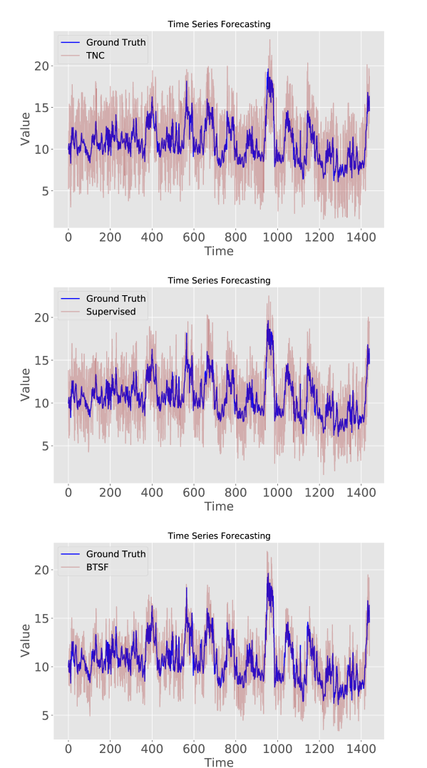
Figure 9: Visualizing long-term forecasting results of length 1440 on ETT dataset.

We evaluate our algorithm with other methods on time series forecasting task in both short-term and long-term settings, following Zhou et al. (2021). A decoder is added on top of learned representations to make predictive outputs. Specifically, we train a linear regression model with L2 norm penalty and use informer (Zhou et al., 2021) as our supervised comparison method. We use two metrics to evaluate the forecasting performance, Mean Square Error (MSE) and Mean Absolute Error (MAE). Table 2 demonstrates that our BTSF has the least forecasting error of different prediction lengths (short/long) across the datasets. In addition, BTSF outperforms existing methods including supervised one in a large margin especially for long time series prediction. It is noted that BTSF gets a better performance when the length of datasets increases due to the better use of global context, which makes BTSF fully capture the long-term dependencies in long time series. More visualization results of time series forecasting are in Appendix B.2, Fig.8 and Fig.9.

Time-Series Anomaly Detection.

To the best of our knowledge, we are the first to evaluate on anomaly detection (Su et al., 2019; Hundman et al., 2018; Goh et al., 2016; Mathur & Tippenhauer, 2016; Braei & Wagner, 2020). The results of this task assessment reflect how well the model capture the temporal trends and how sensitive to the outlier the model is for time series. We add a decoder on top of representations learned by models and reconstruct the input time series and follow the evaluation settings of Audibert et al. (2020). For each input data point ${\bm{x}}_{t}$ and reconstructed one $\hat{{\bm{x}}}_{t}$, if $|\hat{{\bm{x}}}_{t}-{\bm{x}}_{t}|>\tau$ ($\tau$ is a predefined threshold), ${\bm{x}}_{t}$ is an outlier. Precision (P), Recall (R), and F1 score (F1) were used to evaluate anomaly detection performance and we just list the results of F1 metric here (see Appendix B for more results of P and R metrics). Table 3 illustrates that BTSF achieves new SOTA across all datasets and especially surpasses the supervised results by a large margin. It conveys that BTSF is more sensitive to the outliers in time series since it captures long-term dynamics and expresses the fine-grained information through iterative bilinear fusion.

5 Analysis

Comparisons about Time-Series Augmentation Methods.

To further prove the effectiveness of our instance-level augmentation (dropout), we compare our method with 12 other augmentation policies as mentioned in Iwana & Uchida (2021a): Jittering, Rotation, Scaling, Magnitude Warping, Permutation, Slicing, Time Warping, Window Warping, SPAWNER (Kamycki et al., 2020), Weighted DTW Barycentric Averaging (wDBA) (Forestier et al., 2017), Random Guided Warping (RGW) (Iwana & Uchida, 2021b) and Discriminative Guided Warping (DGW) (Iwana & Uchida, 2021b). The classification accuracy comparisons of different augmentations on HAR datasets are illustrated in Figure 3. It is noted that proposed instance-level augmentation (dropout) has a best performance in both average accuracy and variance, which demonstrates dropout is more accurate and more stable for unsupervised representation learning in time series.

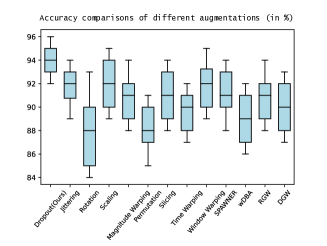
Figure 3: Classification accuracies and variances of different augmentations on HAR dataset.

Impact of Iterative Bilinear Fusion

To investigate the impact of iterative bilinear fusion in BTSF, we follow the experiment as illustrated in Section 1. We apply the learned representations of models to the classification task and make statistics about false predictions by only using temporal or spectral feature respectively. Specifically, we use the feature out of $\operatorname{S2T}$ and $\operatorname{T2S}$ module as temporal and spectral feature respectively. From Table 4, we find that after adding iterative bilinear fusion, BTSF not only gets a large promotion in accuracy but also achieves a good alignment between temporal and spectral domain with a overlap percentage of 96.60%, much higher than existing works (around 30%). Therefore, our designed iterative bilinear fusion make an effective interaction between two domains and it is vital for final prediction accuracy. More ablation studies about BTSF are in Appendix A.

Table 4: Statistics about false predictions of all test samples on HAR dataset

	Only Temporal	Only Spectral	Overlap (% by Temporal, % by Spectral)
SRL	1073	1174	349 (32.53%, 29.73%)
CPC	401	448	106 (26.43%, 23.66%)
TS-TCC	354	383	107 (30.23%, 27.94%)
TNC	346	376	115 (33.24%, 30.59%)
BTSF	159	163	152 (96.60%, 93.25%)

Visualization.

To make assessments about the clusterability of learned representations in the encoding space, we visualize the feature distribution by using t-SNE (Van der Maaten & Hinton, 2008). It is noted that if the information of the latent state is properly learned and encoded by the model, the representations from the same underlying state should cluster together. Figure 4 shows the comparisons about representations distribution of different models. It demonstrates that the representations learned by proposed BTSF from the same hidden state are better than the other approaches. The visualization results further prove the superior representation ability of our model. In Addition, we have evaluated on the all univariate time series datasets: the UCR archive. The corresponding critical difference diagram is shown in Figure 5. The BTSF significantly outperforms the other approaches with an average rank of almost 1.3.

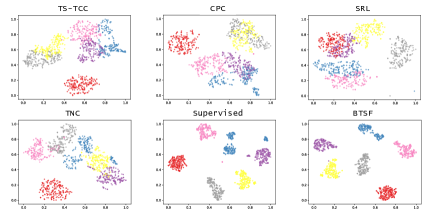
Figure 4: T-SNE visualization of signal representations for HAR dataset.

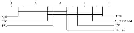
Figure 5: Critical difference diagram showing pairwise statistical difference comparison of BTSF and previous methods on the UCR archive.

Alignment and Uniformity.

To make a comprehensive assessment of the representations, we evaluate the two properties of learned representations, alignment and uniformity (Wang & Isola, 2020). Alignment is used to measure the similarities of features between similar samples, which means features of a positive pair should be invariant to the noise. Uniformity assumes that a well-learned feature distribution should preserve maximal information as much as possible. It makes sense that well-generalized feature representations not only minimize the intra-similarities of positive pairs and enlarge the inter-distances of negative pairs but also keep the feature distributed uniformly to retain enough information. Therefore we follow Wang & Isola (2020) to make the assessments. Figure 6 and Figure 7 show the results of alignment and uniformity respectively. Compared with previous SOTA TNC and supervised results, our BTSF gets the highest mean value about feature distance of positive pairs, which means that BTSF achieves the best alignment. Additionally, the feature extracted BTSF is evenly distributed in the encoding space which preserves maximal information of the data, much better than TNC and supervised models.

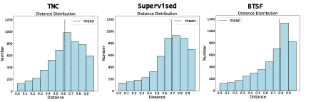
Figure 6: Distance distribution of positive pairs for assessing alignment. Our BTSF is well aligned.

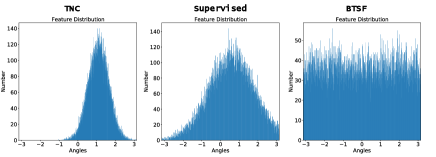
Figure 7: Feature distribution of samples in different classes on the normalized surface area for assessing uniformity. Features extracted by BTSF are evenly distributed.

6 Conclusion

In this paper, we propose Bilinear Temporal-Spectral Fusion (BTSF) for unsupervised time series representation learning. We revisit existing segment-level contrastive learning methods and conclude that they all fail to leverage global contextual information due to the segment-level augmentation (time slicing) and are unable to use temporal-spectral relations for enhancing representation learning. First, we utilize instance-level augmentation which use the entire time series as input and apply dropout to generate different views for training. Second, we devise iterative bilinear temporal-spectral fusion and refine the feature representation in a fuse-and-squeeze manner for time series. The extensive experiments on classification, forecasting and anomaly detection downstream tasks have been conducted and the results demonstrates the superior performance of our BTSF. BTSF surpasses existing unsupervised learning models for time series in a large margin including the supervised model.

Appendix A More ablation studies

To quantify the promotion of each module in BTSF, we make a specific ablation study where all experiments are conducted on HAR dataset and results are in Table 5. We use TNC as a baseline which applies time slicing as augmentation with accuracy of 88.3%. We could find that our instance-level augmentation (dropout) is better than segment-level augmentation (slicing) and layer-wise dropout (adding dropout in internal layers) has a promotion by 1.5% compared with slicing. However, we do not apply layer-wise dropout in aforementioned experiments for fair comparisons otherwise our BTSF will have better performance. Besides, incorporating spectral feature with temporal feature by using summation or concatenation will also improve the results, which illustrates the necessity of cross-domain interaction. The accuracy is obviously promoted by 2%$\sim$3% when involving temporal and spectral information with bilinear fusion, and iterative operation will further improve the performance by enhancing and refining the temporal-spectral interaction. In conclusion, instance-level augmentation (dropout) and iterative bilinear fusion are two main modules of BTSF which largely improve the generalization ability of unsupervised learned representations with accuracy of 94.6%, an improvement of 6.3% to baseline.

Table 5: Ablation experiments of BTSF.

Accuracy	Temporal	Spectral	Sum/Concat	Bilinear	Iterative Bilinear
Slicing	88.3	86.7	88.7	90.7	91.5
Dropout	89.4	88.4	89.8	92.4	94.6
Layer-Wise Dropout	89.8	89.1	90.4	93.1	95.4

Studies of hyperparameters

In the proposed BTSF, there are some hyperparameters needed to be carefully set, the dropout rate, temperature number $\tau$ and the loops number of iterative bilinear fusion. Table 6 illustrates that when the rate is set to 0.1, BTSF acquires the best performance since setting too high value would lose the original properties of time series and setting too low value would bring about representation collapse. Table 7 demonstrates that when $\tau$ is set to 0.05 , BTSF has the best performance. It is reasonable that proper value of $\tau$ would promote the optimization of training process and make representations more discriminative with the adjustment. We also run the experiments of loops number of iterative bilinear fusion, and we conclude that our iterative bilinear fusion is effective and its performance converges after just three loops.

Table 6: Ablation experiments of dropout rate

dropout rate	p=0.01	p=0.05	p=0.1	p=0.15	p=0.2	p=0.3
HAR	90.29	92.78	94.63	93.36	91.21	88.07
Sleep-EDF	82.76	85.34	87.45	86.01	83.44	80.92

Table 7: Ablation experiments on temperature number $\tau$.

$\tau$	0.001	0.01	0.05	0.1	1
HAR	90.04	92.91	94.63	93.04	91.85
Sleep-EDF	82.69	84.82	87.45	85.11	83.28

Appendix B Datasets descriptions and more experiments

In all experiments, we use Pytorch 1.8.1 (Paszke et al., 2017) and train all the models on a GeForce RTX 2080 Ti GPU with CUDA 10.2. We apply an Adam optimizer (Kingma & Ba, 2017) with a learning rate of 3e-4, weight decay of 1e-4 and batch size is set to 256. In this part, we would introduce all the datasets used in our experiments which involve three kinds of downstream tasks, time series classification, forecasting and anomaly detection. The definitions of downstream tasks are detailed in the following:

• Time Series Classification: Given the univariate time series $\{x_{1},x_{2},\dots,x_{T}\}$ or multivariate time series $\{{\bm{x}}_{1},{\bm{x}}_{2},\dots,{\bm{x}}_{D}\}$ as input, time series classification is to classify the input consisting of real-valued observations to a certain class.

• Time Series Forecasting: Given the past univariate observations $\{x_{t-T_{1}+1},\dots,x_{t}\}$ or multivariate ones $\{{\bm{x}}_{t-T_{1}+1},\dots,{\bm{x}}_{t}\}$ as input, time series forecasting aims to predict the future data points $\{x_{t+1},x_{t+2},\dots,x_{t+T_{2}}\}$ or $\{{\bm{x}}_{t+1},{\bm{x}}_{t+2},\dots,{\bm{x}}_{t+T_{2}}\}$ based on the input.

• Time Series Anomaly Detection: Given the univariate time series $\{x_{1},x_{2},\dots,x_{T}\}$ or multivariate time series $\{{\bm{x}}_{1},{\bm{x}}_{2},\dots,{\bm{x}}_{D}\}$ as input, time series anomaly detection is to find out which point ($\hat{x_{i}}$ or $\hat{{\bm{x}}_{i}}$) or subsequence ($\{\hat{x_{1}},\hat{x_{2}},\dots,\hat{x_{T}}\}$ or $\{\hat{{\bm{x}}_{1}},\hat{{\bm{x}}_{2}},\dots,\hat{{\bm{x}}_{T}}\}$) of the input behaves unusually when compared either to the other values in the time series (global outlier) or to its neighboring points (local outlier).

Data Preprocessing

Following Franceschi et al. (2019); Zhou et al. (2021), for univariate time series classification task, we normalize datasets using z-score so that the set of observations for each dataset has zero mean and unit variance. For multivariate time series classification task, each variable is normalized independently using z-score. For forecasting tasks, all reported metrics are calculated based on the normalized time series.

B.1 Classification

In the time series classification task, we choose several popular benchmarks which are widely used in previous works. They are Human Activity Recognition (HAR) (Anguita et al., 2013), Sleep Stage Classification (Sleep-EDF) (Goldberger et al., 2000), Epilepsy Seizure Prediction (Andrzejak et al., 2001), ECG Waveform (Moody, 1983). The detailed introduction to these datasets are as follows:

Human Activity Recognition

HAR dataset contains 30 individual subjects which provide six activities for each subject. These six activities are walking, walking upstairs, downstairs, standing, sitting, and lying down. The data of HAR is collected by sensors with a sampling rate of 50 HZ and the collected signals record the continuous activity of every subject.

Sleep Stage Classification

The dataset is designed for EEG signal classification task where each signal belongs to one of five categories: Wake (W), Non-rapid eye movement (N1, N2, N3) and Rapid Eye Movement (REM). And the Sleep-EDF dataset collects the PSG for the whole night, and we just used a single EEG channel, following previous works (Eldele et al., 2021a).

Epilepsy Seizure Prediction

The Epileptic Seizure Prediction dataset contains EEG signals which are collected from 500 subjects. The brain activity for each subject was recorded for 23.6 seconds. Additionally, the original classes of the dataset are five, and we preprocess the dataset for classification task like Eldele et al. (2021b).

ECG Waveform

The ECG Waveform is a real-world clinical dataset, it includes 25 long-term Electrocardiogram (ECG) recordings (10 hours in duration) of human subjects with atrial fibrillation. Besides, it contains two ECG signals with a sampling rate of 250HZ.

Table 8: More comparisons of classification results about BTSF and previous work, results of TST (Zerveas et al., 2021), Rocket (Dempster et al., 2020) and Supervised (Zerveas et al., 2021) are quoted from TST for fair comparisons.

Methods	TST	Rocket	Supervised	BTSF
EthanolConcentration	32.6	45.2	33.7	49.4
FaceDetection	68.9	64.7	68.1	73.0
Handwriting	35.9	58.8	30.5	62.3
Heartbeat	77.6	75.6	77.6	84.7
JapaneseVowels	99.7	96.2	99.4	99.8
InsectWingBeat	68.7	-	68.4	78.3
PEMS-SF	89.6	75.1	91.9	95.7
SelfRegulationSCP1	92.2	90.8	92.5	96.5
SelfRegulationSCP2	60.4	53.3	58.9	64.9
SpokenArabicDigits	99.8	71.2	99.3	99.8
UWaveGestureLibrary	91.3	94.4	90.3	97.1
Avg Accuracy	74.8	72.5	74.2	82.0
Avg Rank	1.7	2.3	1.7	1.2

Table 9: More comparisons of classification results of ESP dataset.

Methods		Epilepsy Seizure Prediction
		Accuracy	AUPRC
Supervised		96.32$\pm$0.38	0.97$\pm$0.65
KNN		87.96$\pm$1.32	0.89$\pm$1.04
SRL		94.65$\pm$0.97	0.95$\pm$0.86
CPC		96.61$\pm$0.43	0.97$\pm$0.69
TS-TCC		97.23$\pm$0.10	0.98$\pm$0.21
TNC		96.15$\pm$0.33	0.96$\pm$0.45
BTSF		99.01$\pm$0.12	0.99$\pm$0.06

Table 8 shows the comparison results between BTSF with recent works following their evaluation protocols. The results show that BTSF significantly outperforms them in a large margin. Table 9 shows the classification results of Epileptic Seizure Prediction datasets. From the illustrated results, we conclude that our BTSF gets the best performance and exceeds other methods by a large margin in univariate and multivariate time series classification tasks.

B.2 Forecasting

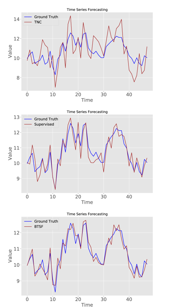
Figure 8: Visualizing forecasting results of length 48 on ETT dataset.

In Section 4, we conduct experiments on four datasets about time series forecasting, including two collected real-world datasets for long sequence time-series forecasting (LSTF) problem and one public benchmark dataset as in Zhou et al. (2021). The detailed introduction to these datasets are as follows:

Electricity Transformer Temperature (ETT)

The ETT is a crucial indicator in the electric power long-term deployment. The 2-year data was collected from two separated counties in China, which was first used to investigate the granularity on the LSTF problem with each data point containing the target value ”oil temperature” and six power load features. ETTh1 , ETTh2 and ETTm1 represent for 1-hour-level and 15-minute-level respectively.

Weather

This dataset contains local climatological data for about 1,600 U.S. places, 4 years from 2010 to 2013, where data points are collected every 1 hour with each data point consisting of the target value “wet bulb” and 11 climate features.

We run the forecasting tasks about prediction length of 48 and 1440 on ETT dataset and visualize the forecasting results of BTSF, TNC and supervised models. From Figure 8 and 9, we could find that our BTSF achieves the best forecasting results under both short-term and long-term settings since it adequately leverages the global context and utilize temporal-spectral relations which are helpful in producing more accurate predictive representations.

B.3 Anomaly detection

In Section 4, we conduct extensive experiments about time series anomaly detection on five widely used datasets, which are all public available. The detailed introduction to these datasets are illustrated as follows:

Secure Water Treatment (SWaT)

The SWaT dataset is a scaled down version of a real-world industrial water treatment plant producing filtered water (Goh et al., 2016). The collected dataset (Mathur & Tippenhauer, 2016) consists of 11 days of continuous operation: 7 days collected under normal operations and 4 days collected with attack scenarios.

Water Distribution (WADI)

This dataset is collected from an extension of the SWaT tesbed. It consists of 16 days of continuous operation: 14 days were collected under normal operation and 2 days with attack scenarios.

Server Machine Dataset (SMD)

This dataset is a 5-week-long dataset from a large internet company which was collected and made publicly available (Su et al., 2019). It contains data from 28 server machines with each one monitored by m=33 metrics. SMD is divided into two subsets of equal size: the first half is the training set and the second half is the testing set.

Soil Moisture Active Passive (SMAP) and Mars Science Laboratory (MSL)

SMAP and MSL are two real-world public datasets, expert-labeled datasets from NASA (Hundman et al., 2018).

References

- Andrzejak et al. (2001) Andrzejak, R. G., Lehnertz, K., Mormann, F., Rieke, C., David, P., and Elger, C. E. Indications of nonlinear deterministic and finite-dimensional structures in time series of brain electrical activity: Dependence on recording region and brain state. Physical Review E, 64(6):061907, 2001.
- Anguita et al. (2013) Anguita, D., Ghio, A., Oneto, L., Parra, X., Reyes-Ortiz, J. L., et al. A public domain dataset for human activity recognition using smartphones. In Esann, volume 3, pp. 3, 2013.
- Audibert et al. (2020) Audibert, J., Michiardi, P., Guyard, F., Marti, S., and Zuluaga, M. A. Usad: Unsupervised anomaly detection on multivariate time series. In Proceedings of the 26th ACM SIGKDD International Conference on Knowledge Discovery & Data Mining, pp. 3395–3404, 2020.
- Bai et al. (2018) Bai, S., Kolter, J. Z., and Koltun, V. An empirical evaluation of generic convolutional and recurrent networks for sequence modeling. arXiv preprint arXiv:1803.01271, 2018.
- Bayer et al. (2021) Bayer, J., Soelch, M., Mirchev, A., Kayalibay, B., and van der Smagt, P. Mind the gap when conditioning amortised inference in sequential latent-variable models. arXiv preprint arXiv:2101.07046, 2021.
- Braei & Wagner (2020) Braei, M. and Wagner, S. Anomaly detection in univariate time-series: A survey on the state-of-the-art. arXiv preprint arXiv:2004.00433, 2020.
- Chen et al. (2020a) Chen, T., Kornblith, S., Norouzi, M., and Hinton, G. A simple framework for contrastive learning of visual representations. In International conference on machine learning, pp. 1597–1607. PMLR, 2020a.
- Chen et al. (2020b) Chen, T., Kornblith, S., Norouzi, M., and Hinton, G. A simple framework for contrastive learning of visual representations. In Proceedings of the 37th International Conference on Machine Learning, volume 119 of Proceedings of Machine Learning Research, pp. 1597–1607, 13–18 Jul 2020b.
- Chen et al. (2013) Chen, Y., Hu, B., Keogh, E., and Batista, G. E. Dtw-d: time series semi-supervised learning from a single example. In Proceedings of the 19th ACM SIGKDD international conference on Knowledge discovery and data mining, pp. 383–391, 2013.
- Choi et al. (2016) Choi, E., Bahadori, M. T., Searles, E., Coffey, C., Thompson, M., Bost, J., Tejedor-Sojo, J., and Sun, J. Multi-layer representation learning for medical concepts. In Proceedings of the 22nd ACM SIGKDD International Conference on Knowledge Discovery and Data Mining, pp. 1495–1504, 2016.
- Chung et al. (2015) Chung, J., Kastner, K., Dinh, L., Goel, K., Courville, A. C., and Bengio, Y. A recurrent latent variable model for sequential data. Advances in neural information processing systems, 28:2980–2988, 2015.
- Deb et al. (2017) Deb, C., Zhang, F., Yang, J., Lee, S. E., and Shah, K. W. A review on time series forecasting techniques for building energy consumption. Renewable and Sustainable Energy Reviews, 74:902–924, 2017.
- Dempster et al. (2020) Dempster, A., Petitjean, F., and Webb, G. I. Rocket: exceptionally fast and accurate time series classification using random convolutional kernels. Data Mining and Knowledge Discovery, 34(5):1454–1495, 2020.
- Denton & Birodkar (2017) Denton, E. and Birodkar, V. Unsupervised learning of disentangled representations from video. arXiv preprint arXiv:1705.10915, 2017.
- Eldele et al. (2021a) Eldele, E., Chen, Z., Liu, C., Wu, M., Kwoh, C.-K., Li, X., and Guan, C. An attention-based deep learning approach for sleep stage classification with single-channel eeg. IEEE Transactions on Neural Systems and Rehabilitation Engineering, 29:809–818, 2021a.
- Eldele et al. (2021b) Eldele, E., Ragab, M., Chen, Z., Wu, M., Kwoh, C. K., Li, X., and Guan, C. Time-series representation learning via temporal and contextual contrasting. arXiv preprint arXiv:2106.14112, 2021b.
- Esling & Agon (2012) Esling, P. and Agon, C. Time-series data mining. ACM Computing Surveys (CSUR), 45(1):1–34, 2012.
- Forestier et al. (2017) Forestier, G., Petitjean, F., Dau, H. A., Webb, G. I., and Keogh, E. Generating synthetic time series to augment sparse datasets. In 2017 IEEE international conference on data mining (ICDM), pp. 865–870. IEEE, 2017.
- Fraccaro et al. (2016) Fraccaro, M., Sønderby, S. K., Paquet, U., and Winther, O. Sequential neural models with stochastic layers. arXiv preprint arXiv:1605.07571, 2016.
- Franceschi et al. (2019) Franceschi, J.-Y., Dieuleveut, A., and Jaggi, M. Unsupervised scalable representation learning for multivariate time series. Advances In Neural Information Processing Systems 32 (Nips 2019), 32(CONF), 2019.
- Goh et al. (2016) Goh, J., Adepu, S., Junejo, K. N., and Mathur, A. A dataset to support research in the design of secure water treatment systems. In International conference on critical information infrastructures security, pp. 88–99. Springer, 2016.
- Goldberger et al. (2000) Goldberger, A. L., Amaral, L. A., Glass, L., Hausdorff, J. M., Ivanov, P. C., Mark, R. G., Mietus, J. E., Moody, G. B., Peng, C.-K., and Stanley, H. E. Physiobank, physiotoolkit, and physionet: components of a new research resource for complex physiologic signals. circulation, 101(23):e215–e220, 2000.
- Gutmann & Hyvärinen (2010) Gutmann, M. and Hyvärinen, A. Noise-contrastive estimation: A new estimation principle for unnormalized statistical models. In Teh, Y. W. and Titterington, M. (eds.), Proceedings of the Thirteenth International Conference on Artificial Intelligence and Statistics, volume 9 of Proceedings of Machine Learning Research, pp. 297–304, Chia Laguna Resort, Sardinia, Italy, 13–15 May 2010.
- Gutmann & Hyvärinen (2012) Gutmann, M. U. and Hyvärinen, A. Noise-contrastive estimation of unnormalized statistical models, with applications to natural image statistics. Journal of Machine Learning Research, 13(2), 2012.
- Hundman et al. (2018) Hundman, K., Constantinou, V., Laporte, C., Colwell, I., and Soderstrom, T. Detecting spacecraft anomalies using lstms and nonparametric dynamic thresholding. In Proceedings of the 24th ACM SIGKDD international conference on knowledge discovery & data mining, pp. 387–395, 2018.
- Hyvarinen & Morioka (2016) Hyvarinen, A. and Morioka, H. Unsupervised feature extraction by time-contrastive learning and nonlinear ica. arXiv preprint arXiv:1605.06336, 2016.
- Iwana & Uchida (2021a) Iwana, B. K. and Uchida, S. An empirical survey of data augmentation for time series classification with neural networks. Plos one, 16(7):e0254841, 2021a.
- Iwana & Uchida (2021b) Iwana, B. K. and Uchida, S. Time series data augmentation for neural networks by time warping with a discriminative teacher. In 2020 25th International Conference on Pattern Recognition (ICPR), pp. 3558–3565. IEEE, 2021b.
- Kamycki et al. (2020) Kamycki, K., Kapuscinski, T., and Oszust, M. Data augmentation with suboptimal warping for time-series classification. Sensors, 20(1):98, 2020.
- Kingma & Ba (2017) Kingma, D. P. and Ba, J. Adam: A method for stochastic optimization, 2017.
- Krishna & Murty (1999) Krishna, K. and Murty, M. N. Genetic k-means algorithm. IEEE Transactions on Systems, Man, and Cybernetics, Part B (Cybernetics), 29(3):433–439, 1999.
- Krishnan et al. (2017) Krishnan, R., Shalit, U., and Sontag, D. Structured inference networks for nonlinear state space models. In Proceedings of the AAAI Conference on Artificial Intelligence, volume 31, 2017.
- Lan et al. (2021) Lan, X., Ng, D., Hong, S., and Feng, M. Intra-inter subject self-supervised learning for multivariate cardiac signals, 2021.
- Längkvist et al. (2014) Längkvist, M., Karlsson, L., and Loutfi, A. A review of unsupervised feature learning and deep learning for time-series modeling. Pattern Recognition Letters, 42:11–24, 2014.
- Laptev et al. (2015) Laptev, N., Amizadeh, S., and Flint, I. Generic and scalable framework for automated time-series anomaly detection. In Proceedings of the 21th ACM SIGKDD International Conference on Knowledge Discovery and Data Mining, pp. 1939–1947, New York, NY, USA, 2015.
- Lei et al. (2017) Lei, Q., Yi, J., Vaculin, R., Wu, L., and Dhillon, I. S. Similarity preserving representation learning for time series clustering. arXiv preprint arXiv:1702.03584, 2017.
- Liu et al. (2021) Liu, X., Liang, Y., Zheng, Y., Hooi, B., and Zimmermann, R. Spatio-temporal graph contrastive learning. arXiv preprint arXiv:2108.11873, 2021.
- Lyu et al. (2018) Lyu, X., Hueser, M., Hyland, S. L., Zerveas, G., and Raetsch, G. Improving clinical predictions through unsupervised time series representation learning. arXiv preprint arXiv:1812.00490, 2018.
- Ma et al. (2019) Ma, Q., Zheng, J., Li, S., and Cottrell, G. W. Learning representations for time series clustering. Advances in neural information processing systems, 32:3781–3791, 2019.
- Malhotra et al. (2017) Malhotra, P., TV, V., Vig, L., Agarwal, P., and Shroff, G. Timenet: Pre-trained deep recurrent neural network for time series classification. arXiv preprint arXiv:1706.08838, 2017.
- Mathur & Tippenhauer (2016) Mathur, A. P. and Tippenhauer, N. O. Swat: A water treatment testbed for research and training on ics security. In 2016 international workshop on cyber-physical systems for smart water networks (CySWater), pp. 31–36. IEEE, 2016.
- Mikolov et al. (2013) Mikolov, T., Chen, K., Corrado, G., and Dean, J. Efficient estimation of word representations in vector space. arXiv preprint arXiv:1301.3781, 2013.
- Moody (1983) Moody, G. A new method for detecting atrial fibrillation using rr intervals. Computers in Cardiology, pp. 227–230, 1983.
- Oord et al. (2018) Oord, A. v. d., Li, Y., and Vinyals, O. Representation learning with contrastive predictive coding. arXiv preprint arXiv:1807.03748, 2018.
- Oreshkin et al. (2020) Oreshkin, B. N., Carpov, D., Chapados, N., and Bengio, Y. N-beats: Neural basis expansion analysis for interpretable time series forecasting. In International Conference on Learning Representations, 2020.
- Pagliardini et al. (2018) Pagliardini, M., Gupta, P., and Jaggi, M. Unsupervised learning of sentence embeddings using compositional n-gram features. In Proceedings of the 2018 Conference of the North American Chapter of the Association for Computational Linguistics: Human Language Technologies, Volume 1 (Long Papers), pp. 528–540, 2018.
- Paszke et al. (2017) Paszke, A., Gross, S., Chintala, S., Chanan, G., Yang, E., DeVito, Z., Lin, Z., Desmaison, A., Antiga, L., and Lerer, A. Automatic differentiation in pytorch. 2017.
- Srivastava et al. (2014) Srivastava, N., Hinton, G., Krizhevsky, A., Sutskever, I., and Salakhutdinov, R. Dropout: A simple way to prevent neural networks from overfitting. Journal of Machine Learning Research, 15(56):1929–1958, 2014.
- Su et al. (2019) Su, Y., Zhao, Y., Niu, C., Liu, R., Sun, W., and Pei, D. Robust anomaly detection for multivariate time series through stochastic recurrent neural network. In Proceedings of the 25th ACM SIGKDD International Conference on Knowledge Discovery & Data Mining, pp. 2828–2837, 2019.
- Tonekaboni et al. (2021) Tonekaboni, S., Eytan, D., and Goldenberg, A. Unsupervised representation learning for time series with temporal neighborhood coding. arXiv preprint arXiv:2106.00750, 2021.
- Van der Maaten & Hinton (2008) Van der Maaten, L. and Hinton, G. Visualizing data using t-sne. Journal of machine learning research, 9(11), 2008.
- Wang & Isola (2020) Wang, T. and Isola, P. Understanding contrastive representation learning through alignment and uniformity on the hypersphere. In International Conference on Machine Learning, pp. 9929–9939. PMLR, 2020.
- Wang & Gupta (2015) Wang, X. and Gupta, A. Unsupervised learning of visual representations using videos. In Proceedings of the IEEE international conference on computer vision, pp. 2794–2802, 2015.
- Yue et al. (2021a) Yue, Z., Wang, Y., Duan, J., Yang, T., Huang, C., Tong, Y., and Xu, B. Ts2vec: Towards universal representation of time series. arXiv preprint arXiv:2106.10466, 2021a.
- Yue et al. (2021b) Yue, Z., Wang, Y., Duan, J., Yang, T., Huang, C., and Xu, B. Learning timestamp-level representations for time series with hierarchical contrastive loss. arXiv preprint arXiv:2106.10466, 2021b.
- Zerveas et al. (2021) Zerveas, G., Jayaraman, S., Patel, D., Bhamidipaty, A., and Eickhoff, C. A transformer-based framework for multivariate time series representation learning. In Proceedings of the 27th ACM SIGKDD Conference on Knowledge Discovery & Data Mining, pp. 2114–2124, 2021.
- Zhou et al. (2021) Zhou, H., Zhang, S., Peng, J., Zhang, S., Li, J., Xiong, H., and Zhang, W. Informer: Beyond efficient transformer for long sequence time-series forecasting, 2021.