Weak pion-production and the second resonance region

Abstract

In this work we report the calculation of the total cross section for pion-production by the dispersion of neutrinos on nucleons. We use a consistent formalism for the intermediate resonance states of spin $\frac{3}{2}$, taking care on the conditions imposed by the invariance on contact transformations and using the Sachs parametrization for the form factors. In addition, we incorporate states in the second resonance region up to 1.6 GeV and implement different approaches for all the dressed resonance propagators. In addition to the $\Delta(1232)$, we include the $N^{*}(1440)$,$N^{*}(1535)$and $N^{*}(1520)$ resonance contributions, and it is shown that this inclusion improve the description of the total cross section regards a model where only the $\Delta$(1230) resonance is considered. Also results for antineutrinos are properly described.

PACS numbers :13.15.+g,13.75.-n,13.60.Le

I INTRODUCTION

In the standard model, neutrinos are massless, but experimental evidence shows that although small, it is not zero. This increases interest in their study as it leads to flavor oscillations, mixture of angles between mass states, violation of quantum numbers, among others. The detection of neutrino masses is the first evidence of physics beyond the standard model. Neutrino physics has been one of the most studied topics in recent years for particle physics. Now, as it is known that neutrinos are massive particles that can oscillate (changing flavor), it is essential to know precisely the cross section in the interaction of the neutrino with nucleons or with a nucleus in the detector. The interaction of neutrinos with nuclei and nucleons have received considerable attention in recent years, stimulated by the needs in the analysis of neutrino experiments giving information about the probability of oscillation. There are several processes for the study of the interaction of neutrinos with nucleons. The dispersion of neutrinos by nucleons can be quasielastic or inelastic producing additional pions together the nucleon in charged current (CC) and neutral current (NC) interactions Llewe72 . CC quasi-elastic (QE) interaction of neutrinos and antineutrinos with nucleons involves the processes $\nu_{\ell}+n\rightarrow p+\ell^{-}$and $\bar{\nu}_{\ell}+p\rightarrow n+\ell^{+}$ respectively where $\ell=e$, $\nu$, $\tau$, and it is used to detect the arriving of neutrinos or antineutrinos to the detectors. The following process in importance to be considered is the CC single pion production (SPP) $\nu_{\ell}+N\rightarrow\ell^{-}+N^{\prime}\pi$ and $\bar{\nu}_{\ell}+N\rightarrow\ell^{+}+N^{\prime}\pi$ , where $N,N^{\prime}=$ $p$, $n$ or the NC one $\nu_{\ell}+N\rightarrow\nu^{\prime}_{\ell}+N^{\prime}\pi$ and $\bar{\nu}_{\ell}+N\rightarrow\bar{\nu}^{\prime}_{\ell}+N^{\prime}\pi$ .

A good understanding of SPP by neutrinos with few-GeV energies is important for current and future oscillation experiments, where pion production is either a signal process when scattering cross sections are analyzed, or a large background for analyses which select QE events. At these energies, the dominant production mechanism is via the production and subsequent decay of hadronic resonances.

The axial form factor(FF) for pion production on free nucleons cannot be constrained by electron scattering data, used normally to get the vector FF, so it relies upon data from Argonne National Laboratory’s $12$ ft bubble chamber (ANL)Rad82 (2) and Brookhaven National Laboratory’s $7$ ft bubble chamber (BNL)Kitagi86 (3). The ANL neutrino beam was produced by focusing 12.4 GeV protons onto a beryllium target. Two magnetic horns were used to focus the positive pions produced by the primary beam in the direction of the bubble chamber, these secondary particles decayed to produce a predominantly $\nu_{\mu}$ peaked at $\sim 0.5$ GeV. The BNL neutrino beam was produced by focusing 29 GeV protons on a sapphire target, with a similar two horn design to focus the secondary particles. The BNL $\nu_{\mu}$ beam had a higher peak energy of $\sim 1.2$ GeV, and was broader than the ANL beam. These experiments will be referenced below in the results section. These datasets differed in normalization by 30–40$\%$ for the leading pion production process $\nu_{\mu}p\rightarrow\mu^{-}p\pi^{+}$, which conduced to large uncertainties in the predictions for oscillation experiments.

It has long been suspected that the discrepancy between ANL and BNL was due to an issue with the normalization of the flux prediction from one or both experiments, and it has been shown by other authors that their published results are consistent within the experimental uncertainties providedGraczyk09 (4, 5). In Ref. wilki14 (6), was presented a method for removing flux normalization uncertainties from the ANL and BNL $\nu_{\mu}p\rightarrow\mu^{-}p\pi^{+}$ measurements by taking ratios with charged current quasielastic (CCQE) event rates in which the normalization cancels. Then, it was obtained a measurement of $\nu_{\mu}p\rightarrow\mu^{-}p\pi^{+}$by multiplying the ratio by an independent measurement of CCQE (which is wellknown for nucleon targets). Using this technique, they found good agreement between the ANL and BNL $\nu_{\mu}p\rightarrow\mu^{-}p\pi^{+}$datasets. Later, they extend that method to include the subdominant $\nu_{\mu}n\rightarrow\mu^{-}p\pi^{0}$ and $\nu_{\mu}n\rightarrow\mu^{-}n\pi^{+}$channelsRodriguez16 (7). This is one of the reasons encourage us to return to the calculation of SPP neutrino-nucleon cross sections. The other reason is that there are many models to describe this process that fail in several aspects namely:
i)There are problems from the formal point of view. Since the pion emission source are excitation and decay of resonances, and many of them are of spin $\frac{3}{2}$, we must keep amplitudes invariant by contact transformations (see below). These transformations change the amount of the spin-$\frac{1}{2}$ spurious contribution in the field that are present by construction. Many works keep the simpler forms of the free and interaction Lagrangians, and the amplitude lacks the mentioned invariance
ii)In addition to the resonances pole contribution(normally referred as resonant terms) to the amplitude, we have background terms coming form cross resonance contributions and non-resonance origin (called usually non resonant terms). Many works do not consider the interference between resonant and background contributions and really it is very important to describe the data.
iii)Another models detach the decay process for the resonance out of the whole weak production amplitude. However, resonances are nonperturbative phenomena associated to the pole of the S-matrix amplitude and one can not detach its production from its decay mechanisms, omitting the details in the propagation.

In this work we calculate the SPP cross section, where we use a consistent formalism for the intermediate resonance states of spin $\frac{3}{2}$. The $\Delta(1232)$ will be described within the Complex Mass Scheme (CMS), obtained from its dressed propagator (see below). In addition, we incorporate states in the second resonance region which includes the $N^{*}(1440),N^{*}(1535),N^{*}(1520)$ resonances treated within a constant width approach . This work is organized as follows: In Section II, summarize the general description of weak interactions and the SPP cross section. In Section III we will introduce the formalism of Rarita -Schwinger for spin-$\frac{3}{2}$ particles, the dressed propagator for them and propose the consistent form of the vertex and the propagator. Also, we introduce the formalism for the $\Delta(1232)$ and resonances of the second region ($N^{*}(1440),N^{*}(1520),N^{*}(1535)$). In Section IV we show the results obtained with our model in the different regimes of the final $W_{\pi N}$ invariant mass. Finally in Section VI we summarize our conclusions.

II Neutrino-nucleon scattering

The CC interaction (we omit other contributions) between a neutrino and a hadron is obtained from the weak Lagrangian

$$\mathscr{\mathcal{L}}_{CC} = \frac{-g}{2\sqrt{2}}\left(J_{lCC}^{\mu}W_{\mu}+J_{hCC}^{\mu}\sqrt{2}\left(\bm{\tau}\mbox{or }\bm{T}^{\dagger}\right)\cdot\bm{W}+h.c.\right)$$ (1)

being the leptonic and hadronic currents respectively

$$J_{lCC}^{\mu} = \sum_{l}\bar{\psi_{l}}\gamma^{\mu}(1-\gamma_{5})\psi_{\nu_{l}},$$

$$J_{hCC}^{\mu} = \bar{\psi}_{h^{\prime}}(V^{\mu}-A^{\mu})\psi_{h},$$ (2)

where the isospin operator $\bm{\tau}$, the ${\bf T^{\dagger}}$ $N\rightarrow R(I=\frac{3}{2})$ excitation one, and the isospin wave functions for the bosons $\bm{W}_{\pm}$( equal to the pions $\boldsymbol{\phi}_{\pm}$), the nucleons $N=p,n$ and resonances R, are defined in the appendix A. Finally we have the $W$ propagator

$$D_{\mu\nu}(p) = \frac{-g_{\mu\nu}+\frac{p_{\mu}p_{\nu}}{m_{W}^{2}}}{p^{2}-m_{W}^{2}}\approx\frac{g_{\mu\nu}}{m_{W}^{2}},$$

being $\frac{g_{\mu\nu}}{m_{W^{2}}}$ the the high mass limit since usually $p^{2}\ll m_{W}^{2}$.

In this work we analyze the CC $\nu N\rightarrow\mu^{-}N^{\prime}\pi$ and $\bar{\nu}N\rightarrow\mu^{+}N^{\prime}\pi$ modes. The total amplitude $\mathcal{M}$ can be expressed from the Lagrangian (1) as (spin and isospin indexes omitted)

$$\mathcal{M} = \frac{ig^{2}}{\left(2\sqrt{2}\right)^{2}}\bar{u}(p_{\mu})(-)i\gamma^{\lambda}(1-\gamma_{{}_{5}})u(p_{\nu})\frac{ig_{\lambda\lambda^{\prime}}}{m_{W}^{2}}V_{ud}\bar{u}(p^{\prime})\mathcal{O}^{\lambda^{\prime}}(p^{\prime},k,p,q)u(p),$$ (3)

where$\frac{g^{2}}{\left(2\sqrt{2}\right)^{2}}=\frac{G_{F}^{2}}{\sqrt{2}}$, $G_{F}=1.16637\times 10^{-5}GeV{}^{-2}$ , $|V_{ud}|=0.9740$, and the 4-momenta are defined as

$$p_{\nu}=(E_{\nu},{\bf p}_{\nu}),\hskip 14.22636ptp_{\mu}=(E_{\mu},{\bf p}_{\mu}),\hskip 14.22636pt\text{k}=(E_{\pi},{\bf k}),\hskip 14.22636ptp=(E_{N},{\bf p}),\qquad p^{\prime}=(E_{{}_{N^{\prime}}},{\bf p}^{\prime})$$

with $E_{i}=\sqrt{|{\bf p}_{i}|^{2}+m_{i}^{2}}$, we set $m_{\nu}=0$, and $\mathcal{O}^{\lambda}$ is the vertex generated by $J_{hCC}^{\mu}$ in the Lagrangian (1). We will built $\bar{u}O^{\lambda}u$ for the $\nu(\bar{\text{$\nu$}})N\rightarrow\mu N^{\prime}\pi$ process with the contributions shown in Fig.1. Clearly, all the Feynman graphs do not necessarily contribute to each of channels as we will analyze.

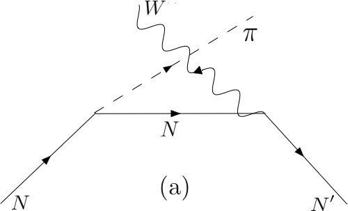
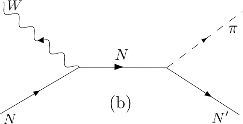
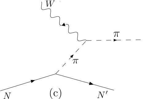
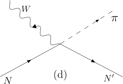
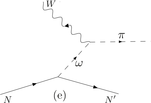
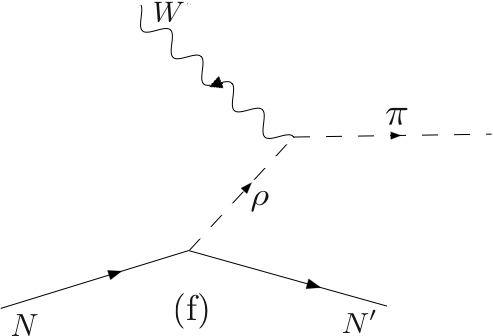
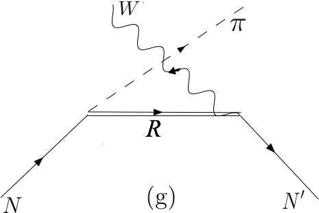
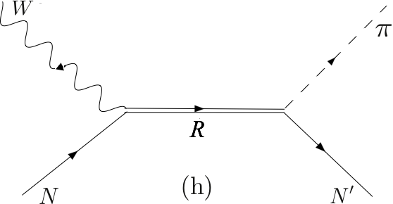
Figure 1: Contributions to the scattering amplitude for the process $\nu(\bar{\text{$\nu$}})N\rightarrow\mu N^{\prime}\pi$. Fig (a)-(g) are the background (B) contributions. Fig (h) are the pole resonant contributions (R). $R$ in the Figure indicates any of the intermediate considered resonances.

We assume a tree-level hadronic amplitudes contributing to the so called background (B) that encloses the nucleon Born terms (Fig. 1(a)-(b)), the meson exchange amplitudes(including the contact term) (Figs. 1(c)-(f)) and the resonance($R)$-crossed term (Fig. 1(g)); the pole resonant contribution (R) is shown in Fig. 1(h) and as we will show the resonance acquires a width (i.e we don’t have only a tree-label amplitude) that avoids the singularity in the propagator by a dressing it at different levels of approximation. In this way, we split the hadronic operator $\mathcal{O}^{\lambda}$ involved in the hadronic amplitude in Eq.(3) as

$$\mathcal{O}^{\lambda} = \mathcal{O}_{\text{B}}+\mathcal{O}_{\text{R}},$$ (4)

where as will be seen $\mathcal{O}_{B,R}$ are built through the Feynman rules obtained from the different effective Lagrangians.

The total cross section for weak SPP in terms of the $\nu N$ center mass (CM) variables for convenience, will be calculated from (we take $\boldsymbol{p}_{\nu}=E_{\nu}\hat{\boldsymbol{k}}$ along the $Z$axis)

$$\sigma(E_{{}_{\nu}}^{\text{CM}}) = \frac{m_{{}_{\mu}}m_{{}_{N}}^{2}}{(2\pi)^{4}E_{{}_{\nu}}^{\text{CM}}\sqrt{s}}\int\limits_{E_{\mu}^{{}^{-}}}^{E_{\mu}^{{}^{+}}}dE_{{}_{\mu}}^{\text{CM}}\int\limits_{E_{\pi}^{{}^{-}}}^{E_{\pi}^{{}^{+}}}dE_{{}_{\pi}}^{\text{CM}}\int\limits_{-1}^{+1}d\cos\theta\int\limits_{0}^{2\pi}d\eta\frac{1}{16}\sum\limits_{\text{spin}}|\mathcal{M}|^{2},$$ (5)

where $\sqrt{s}=\sqrt{(p_{\nu}+p_{N})^{2}}=E_{{}_{\nu}}^{\text{CM}}+E_{{}_{N}}^{\text{CM}}$, the angular variable come from the integration elements $d\Omega_{\mu}=d\cos\theta d\phi$ and $d\Omega_{\pi}=dcos\xi d\eta$ ($d\phi$ integration gives a factor $2\pi$ and $\cos\xi$ is fixed by energy conservation) and

$$E_{{}_{\mu}}^{-} = m_{{}_{\mu}},\>E_{{}_{\mu}}^{{}^{+}}=\frac{s+m_{{}_{\mu}}^{2}-(m_{{}_{N}}+m_{{}_{\pi}})^{2}}{2(E_{{}_{\nu}}^{CM}+E_{{}_{N}}^{\text{CM}})},$$

$$E_{{}_{\pi}}^{\pm} = \frac{(\sqrt{2}-E_{{}_{\mu}}^{CM})(s-2\sqrt{s}E_{{}_{\mu}}^{CM}-\Delta_{m}^{2})\pm A\sqrt{(E_{{}_{\mu}}^{CM})^{2}-m_{\mu}^{2}}}{2(s-2\sqrt{s}E_{{}_{\mu}}^{CM}+m_{{}_{\mu}}^{2})},$$ (6)

with

$$A = \sqrt{(s-2\sqrt{s}E_{{}_{\mu}}^{CM}-\Delta_{m}^{2})^{2}-4m_{{}_{\pi}}^{2}(s-2\sqrt{s}E_{{}_{\mu}}^{CM}+m_{{}_{\mu}}^{2})},$$

$$\Delta_{m}^{2} = m_{{}_{N}}^{2}-m_{{}_{\mu}}^{2}-m_{{}_{\pi}}^{2}.$$ (7)

The neutrino energy CM energy is related with the laboratory one as

$$E_{{}_{\nu}}^{CM} =\frac{m_{N}E_{\text{$\nu$}}^{Lab}}{\sqrt{s}} \frac{m_{{}_{N}}E_{{}_{\nu}}^{Lab}}{\sqrt{2E_{{}_{\nu}}^{Lab}m_{{}_{N}}+m_{{}_{N}}^{2}}}.$$ (8)

It is wellknown that the hadronic currents $J_{hCC}^{\lambda}$ have a vector-axial structure $J_{hCC}^{\lambda}\equiv V^{\lambda}-A^{\lambda}$. In terms of the vector current, the electromagnetic one is written as $J_{\text{elec}}^{\lambda}=V_{\text{isoscalar}}^{\lambda}+V_{3}^{\lambda}$ ($V_{3}^{\lambda}=\tau_{3}\frac{\gamma^{\lambda}}{2}$ for a nucleon or R($I=\frac{1}{2})$, and $V^{\lambda}T_{3}^{\dagger}$ for the $R(I=\frac{3}{2})$) and the weak vector CC is obtained through the CVC hypothesis ($\tau_{3},T_{3}^{\dagger}\rightarrow\sqrt{2}\tau_{\pm},\sqrt{2}T_{\pm}^{\dagger}$) as $V_{\pm}^{\lambda}\equiv\mp(V_{1}^{\lambda}\pm iV_{2}^{\lambda})=\sqrt{2}\bm{V}\cdot\bm{W}_{\pm}$. In the same way it is also possible to get information on different contributions to the vector current in $\mathcal{\mathcal{M_{B}}}$ as the effective $WM\rightarrow\pi^{\prime}$ (with $M\equiv\pi,\omega$) and the contact $NW\pi\rightarrow N^{\prime}\pi^{\prime}$ vector vertexes. Here the FF are again obtained assuming CVC from the electromagnetic $\gamma M\rightarrow\pi^{\prime}$ and $\gamma N\pi\rightarrow N^{\prime}\pi^{\prime}$ vertexes obtained through the corresponding effective interaction Lagrangians, making the replacement $(\bm{\Phi}_{\pi}^{{}^{\prime}*}\times\bm{\Phi}_{\pi})_{3}\rightarrow\mp[(\bm{\Phi}_{\pi}^{{}^{\prime}*}\times\bm{\Phi}_{\pi})_{1}\pm i(\bm{\Phi_{\pi}}^{{}^{\prime}*}\times\bm{\Phi}_{\pi})_{2}]=\sqrt{2}(\bm{\Phi}_{\pi}^{{}^{\prime}*}\times\bm{\Phi}_{\pi})_{\pm}=\surd 2(\bm{\Phi}_{\pi}^{{}^{\prime}*}\times\bm{\Phi}_{\pi})\cdot\bm{W}_{\pm}$ (the same is valid for the contact vertex changing $\boldsymbol{\Phi}_{\pi}\rightarrow\tau$) for $M=\pi$ or $\boldsymbol{\Phi}_{\pi_{3}}^{{}^{\prime}}\rightarrow\sqrt{2}\bm{\Phi}_{\pi}^{\prime}\cdot\bm{W}_{\pm}$ for $M=\omega$. The $\rho$-exchange in the $\rho W\text{\textrightarrow}\pi$ vertex does not contribute to the vector current since the $\rho-\pi$ current is isoscalar. We assume a phenomenological $\rho W\rightarrow\pi$ axial vertex, where the isospin factor is the same as in the $\pi^{\prime}W\rightarrow\pi$ vector case.

III Resonances

In this section we will show the resonance Lagrangians to built $\mathcal{O}_{R}$ since those used to get $\mathcal{O}_{B}$ are more general and will be referenced from the appendix B.

III.1 Spin $\frac{3}{2}$ resonances

III.1.1 $\Delta$(1232) resonance

This $IJ^{\pi}=\frac{3}{2},\frac{3}{2}^{+}$ positive parity resonance has a three quark orbital momentum and spin $L=0,S=\frac{3}{2}$ and its free most general one-parameter Lagrangian reads

$$\mathcal{L}(A) = \overline{\Psi}_{\mu}(x)\Lambda^{\mu\nu}(A)\Psi_{\nu}(x),$$ (9)

where

$$\Lambda^{\mu\rho}(A) = R_{\hskip 5.69046pt\sigma}^{\mu}(\frac{1+3A}{2})\Lambda^{\sigma\delta}(-\frac{1}{3})R_{\hskip 5.69046pt\delta}^{\rho}(\frac{1+3A}{2}),$$ (10)

$$\Lambda^{\mu\rho}(-\frac{1}{3}) = \left(i\not{\partial}-m_{\Delta}\right)g^{\mu\rho}+i\gamma^{\mu}\not{\partial}\gamma^{\rho}-i\left(\partial^{\mu}\gamma{}^{\rho}+\gamma^{\mu}\partial^{\rho}\right)+m_{\Delta}\gamma^{\mu}\gamma^{\rho},$$

and $R^{\rho\sigma}(a)=g^{\rho\sigma}+a\gamma^{\rho}\gamma^{\sigma}$. We have that $\Psi_{\mu}\equiv\psi\otimes\xi_{\mu}$, where $\psi$ is a Dirac spinor field and $\xi_{\mu}$ is a Dirac 4-vector Kirbach2002 (8). In this way, the field $\Psi_{\mu}$ will contain a physical spin- $\frac{3}{2}$ sector and a spurious spin- $\frac{1}{2}$ sector dragged by construction. The free Lagrangian leads to an equation of motion

$$\Lambda^{\mu\nu}(A)\Psi_{\nu}(x) = 0,$$ (11)

plus certain constraints

$$\partial_{\mu}\Psi^{\mu} = \gamma_{\mu}\Psi^{\mu}=0,$$ (12)

independent of $A$ that fix the $\frac{3}{2}$ component eliminating the redundant $\frac{1}{2}$ contributions. $R^{\rho\sigma}(a)$ changes the proportion of the spurious $\frac{1}{2}$ component of the Rarita Schwinger field $\Psi_{\mu}$ but, due to the mentioned constraints, does not affect the $\frac{3}{2}$ sector. This is the origin of the family of Lagrangians and $\mathcal{L}(A=-\frac{1}{3})$, where $R^{\rho\sigma}(a=0)=g^{\rho\sigma}$, was the original form proposed by Rarita-Schwinger Rarita (9). Also using the properties of $R^{\rho\sigma}$, it should be invariant under the contact transformation

$$\Psi^{\nu} \rightarrow\Psi^{{}^{\prime}\nu}= R_{\mu\nu}(a)\Psi^{\nu},\leavevmode\nobreak\ \leavevmode\nobreak\ A\rightarrow A^{\prime}=\frac{A-2a}{1+4a},$$ (13)

$(a\neq-\frac{1}{4},A\neq-\frac{1}{2})$, to avoid a singularity, and we get $\mathcal{L}(A^{\prime})=\overline{\Psi}_{\mu}^{\prime}(x)\Lambda^{\mu\nu}(A^{\prime})\Psi_{\nu}^{\prime}(x).$ The invariance of the free Lagrangian under the contact transformations means that the physical quantities as energy and momentum should be independent of A. The spin-$\frac{3}{2}$ propagator $G(p,A)^{\beta\nu}$ should satisfy (in momentum space, we replace $i\partial\rightarrow p$),

$$\Lambda(p_{\Delta},A)^{\beta\mu}G^{\Delta}(p_{\Delta},A)_{\beta\nu}=g^{\mu\nu},$$

for any value of $A$ and to keep consistence, it should be transformed as

$$G^{\Delta}(p_{\Delta},A)_{\mu\nu} = R^{-1}(\frac{1+3A}{2})_{\mu\alpha}G^{\Delta\alpha\beta}(p_{\Delta},-\frac{1}{3})R^{-1}(\frac{1+3A}{2})_{\beta\nu}$$ (14)

$$= R^{-1}(-{1\over 2}(1+A))_{\alpha}^{\mu}G^{\Delta}(p_{\Delta},-1)^{\alpha\beta}R^{-1}(-{1\over 2}(1+A))_{\beta}^{\nu}.$$

It can be put in terms of the spin $\frac{3}{2},\frac{1}{2}$ projectors defined in the appendix A, as (omitting Dirac indexes )

$$G_{0}^{\Delta}(p_{\Delta}) \equiv G^{\Delta}(p_{\Delta},-\frac{1}{3})=-\left[\frac{\not{p}_{\Delta}+m}{p_{\Delta}^{2}-m_{\Delta}^{2}}P^{\frac{3}{2}}+\frac{2}{m_{\Delta}^{2}}(\not{p}_{\Delta}+m_{\Delta})P_{11}^{\frac{1}{2}}+\frac{\sqrt{3}}{m_{\Delta}}(P_{12}^{\frac{1}{2}}+P_{21}^{\frac{1}{2}})\right]$$ (15)

$$G^{\Delta}\left(p_{\Delta},-1\right) = -\left[\frac{\not\!p_{\Delta}+m}{p_{\Delta}^{2}-m_{\Delta}^{2}}P^{\frac{3}{2}}-\frac{2}{3m_{\Delta}^{2}}(\not{p}_{\Delta}+m_{\Delta})P_{22}^{\frac{1}{2}}+\frac{1}{\sqrt{3}m_{\Delta}}(P_{12}^{\frac{1}{2}}+P_{21}^{\frac{1}{2}})\right],$$ (16)

where we put in terms of $A=-\frac{1}{3},-1$ since will be the cases to discuss below, or alternatively the developed form

$$G_{{}_{\alpha\beta}}^{\Delta}(p_{\Delta},A) = -\frac{1}{p_{\Delta}^{2}-m_{{}_{\Delta}}^{2}}\Bigg{\{}\left(\not{p}_{\Delta}+m_{{}_{\Delta}}\right)\left[-g_{{}_{\alpha\beta}}+\frac{1}{3}\gamma_{{}_{\alpha}}\gamma_{{}_{\beta}}+\frac{1}{3m_{{}_{\Delta}}}(\gamma_{{}_{\alpha}}p_{{}_{\Delta\beta}}-\gamma_{{}_{\beta}}p_{{}_{\Delta\alpha}})+\frac{2}{3m_{{}_{\Delta}}}p_{{}_{\Delta\alpha}}p_{{}_{\Delta\beta}}\right]$$ (17)

$$- \frac{2(p_{\Delta}^{2}-m_{{}_{\Delta}}^{2})b(A)}{3m_{{}_{\Delta}}^{2}}\left[\gamma_{{}_{\alpha}}p_{{}_{\Delta\beta}}-(b(A)-1)\gamma_{{}_{\beta}}p_{{}_{\Delta\alpha}}-(\frac{b(A)}{2}\not{p}_{\Delta}+(b(A)-1)m_{{}_{\Delta}})\gamma_{{}_{\alpha}}\gamma_{{}_{\beta}}\right]\Bigg{\}},$$

where $b(A)=\frac{A+1}{2A+1}$. Note that (17) is singular at $p^{2}=m_{\Delta}^{2}$, that is when the resonance is on-shell, but we know that it must be dressed trough a self energy and thus this singularity it is avoided as we will discuss below. It is interesting to note that the second A-dependent contribution in brackets disappears for the $\Delta$ on shell, i.e when the constraints filter the $\frac{1}{2}$ contribution. Nevertheless, the resonance appears always off-shell in the presence of interactions, and (12) do not hold. The amplitudes can be defined uniquely, independent of $A$, when the interactions with the spin-$\frac{3}{2}$ field are properly chosen. Consequently, we demand the interaction Lagrangian for the $\frac{3}{2}$ field coupled to a nucleon ($\psi$) and a pseudo-scalar meson ($\phi$) or boson ($W$), as usually appears in a resonance production-decay, be invariant under (13). The most general interaction Lagrangian satisfying such requirement is

$${\cal{L}}_{int}(A,Z)=g_{int}\bar{\Psi}^{\mu}R(\frac{1}{2}(2Z+(1+4Z)A))_{\mu\nu}F^{\nu}(\psi,\phi,W,...)+h.c.,$$ (18)

where $F_{\nu}$ is a function of the fields and its derivatives, $g_{int}$ is the coupling constant and $Z$ a new arbitrary parameter. Using the property $R(a)_{\mu\nu}R(b)_{\lambda}^{\nu}=R(a+b+4ab)_{\mu\lambda}$ it is possible to demonstrate

$$R(\frac{1}{2}(2Z+(1+4Z)A)_{\alpha\beta}=R(\frac{1+3A}{2})_{\alpha\mu}R^{-1}(\frac{1}{2}(1-6Z/(1+4Z))_{\beta}^{\mu}$$ (19)

that would be replaced in Eq.(18) . Note that the A-dependence introduced by the propagator (14) in the $W\psi\rightarrow\phi\psi$ amplitude is canceled by the $R(\frac{1+3A}{2})$ in the vertex generated from (18). That is, for any value of $Z$ we get an $A$-independent amplitude. Then, the value for $Z$ must be chosen for each interaction and fixed by a criteria independent from contact transformations.

For the strong $\Delta\pi N$ interaction Lagrangian we adopt the usual chiral invariant one derivative in the pion field

$$\mathcal{L}_{\Delta N\pi}(A=-\frac{1}{3},Z=\frac{1}{2}) = \frac{f_{\pi N\Delta}}{m_{\pi}}\bar{\psi}\partial[\bm{\Phi}(x)^{\mu}]^{\dagger}\cdot\bm{T}\Psi_{\mu}+\frac{f_{\pi N\Delta}}{m_{\pi}}\bar{\Psi}_{\mu}\bar{\psi}\partial\bm{\Phi}(x)^{\mu}\cdot\bm{T}^{\dagger}\psi,$$ (20)

where the choosing in $Z$ will be explained below, and this Lagrangian enables the definition of the $\Delta\rightarrow\pi N$ vertex

$$V^{\Delta\pi N} =- \frac{f_{\pi N\Delta}}{m_{\pi}}k^{\mu}N^{\dagger}\left(\bm{\phi^{*}}\cdot\bm{T}\right)\Delta,$$ (21)

where we use the prescription $\hat{\Gamma}=i\mathcal{L}$ , $\partial^{\mu}\phi=-ik^{\mu}\phi$ and $i\times propagator$, and a global $i$ in the total amplitudes.

The weak interaction Lagrangian $\hat{\mathcal{L}}_{{}_{WN\Delta}}$ compatible with the free $\hat{\mathcal{L}}_{{}_{\Delta}}$ and the strong interacting Lagrangian $\hat{\mathcal{L}}_{\Delta\pi N}$ that makes possible also a definition of the weak $WN\Delta$ excitation vertex, is Barbero08 (10)(we choose the same $Z$ value)

$$\mathcal{L}_{{}_{WN\Delta}}(A=-\frac{1}{3},Z=\frac{1}{2}) = \bar{i\Psi}^{\mu}(x)\hat{{\mathcal{W}}}_{\mu\nu}\sqrt{2}(\bm{T}^{\dagger}\cdot\bm{W}^{\nu}(x)^{\dagger})\psi(x)+\text{h.c.},$$

with a vertex $W^{WN\Delta}=\left(V^{WN\Delta}+A^{WN\Delta}\right)\sqrt{2}\bm{W}^{*}\cdot\bm{T}^{\dagger}$ being the same $V^{WN\Delta}$ vector vertex as in pion-photo($Q^{2}=0)$Mariano07 (11) and electroproduction applying CVC

$$V_{\nu\mu}^{WN\Delta}(q,p)=[(G_{{}_{M}}(Q^{2})-G_{{}_{E}}(Q^{2}))K_{\nu\mu}^{M}+G_{{}_{E}}(Q^{2})K_{\nu\mu}^{E}+G_{{}_{C}}(Q^{2})K_{\nu\mu}^{C}],$$ (22)

with $Q^{2}=-q^{2}=-m_{\ell}+2E_{\ell}E_{\nu}(p_{\ell}/E_{\ell}\cos\theta_{\nu\ell})>0$ , being $q=p_{l}-p_{\nu}$, and where

$$K_{\nu\mu}^{M} =-\frac{3(m_{{}_{N}}+m_{\Delta})}{2m_{{}_{N}}(m_{{}_{N}}+m_{\Delta})^{2}+Q^{2}}\epsilon_{\nu\mu\alpha\beta}\frac{(p+p_{\Delta})^{\alpha}}{2}q^{\beta},$$

$$K_{\nu\mu}^{E} =\frac{4}{(m_{\Delta}-m_{{}_{N}})^{2}+Q^{2}}\frac{3(m_{{}_{N}}+m_{\Delta})}{2m_{{}_{N}}(m_{{}_{N}}+m_{\Delta})^{2}+Q^{2}}\epsilon_{\nu\lambda\alpha\beta}\frac{(p+p_{{}_{\Delta}})^{\alpha}}{2}q^{\beta}\epsilon_{\mu\gamma\delta}^{\lambda}p_{{}_{\Delta}}^{\gamma}q^{\delta}i\gamma_{{}_{5}}$$

$$K_{\nu\mu}^{C} =\frac{2}{(m_{\Delta}-m_{{}_{N}})^{2}+Q^{2}}\frac{3(m_{{}_{N}}+m_{1520})}{2m_{{}_{N}}(m_{{}_{N}}+m_{\Delta})^{2}+Q^{2}}\left[-q^{2}g_{\alpha\mu}+q_{\alpha}q_{\mu}\right]q_{\nu}\frac{(p+p_{{}_{\Delta}})^{\alpha}}{2}i\gamma_{{}_{5}}.$$ (23)

For the FF we adopt

$$G_{{}_{i}}(Q^{2})=G_{{}_{i}}(0)G_{V}(Q^{2}),$$ (24)

and for the axial contribution we use the model given in Ref.(Barbero08 (10)), which is compatible with $V_{\nu\mu}^{WN\Delta}$ (it could be, in principle, obtained by using $-V_{\nu\mu}^{WN\Delta}\gamma_{{}_{5}}$) and reads

$$A_{\nu\mu}^{WN\Delta}(q,p) = -i\Bigg{[}-D_{{}_{1}}(Q^{2})g_{{}_{\nu\mu}}+\frac{D_{{}_{2}}(Q^{2})}{m_{{}_{N}}^{2}}(p+p_{{}_{\Delta}})^{\alpha}(g_{{}_{\nu\mu}}q_{{}_{\alpha}}-q_{{}_{\nu}}g_{{}_{\alpha\mu}})-$$ (25)

$$- \frac{D_{{}_{3}}(Q^{2})}{m_{{}_{N}}^{2}}p_{\nu}q_{{}_{\mu}}+i\frac{D_{4}(Q^{2})}{m_{{}_{N}}^{2}}\epsilon_{\mu\nu\alpha\beta}(p+p_{{}_{\Delta}})^{\alpha}q^{\beta}\gamma_{{}_{5}}\Bigg{]}.$$

The $G_{{}_{i}}(Q^{2})$ and $D_{{}_{i}}(Q^{2})$ FF will also be described below .

The bare propagator (17) being singular at $p_{\Delta}^{2}=m_{\Delta}^{2}$ should be dressed by the inclusion of a self-energy ($\Sigma$) giving to it a width corresponding to an unstable particle. This self-energy (where usually only Born interaction terms are considered) could include the lowest order $\pi N$ one-loop contribution as well as other higher order $\pi N$ irreducible scattering non-pole contributions consistent with the $\pi N$ scattering amplitude.

The expression for the dressed propagator $G^{\Delta}{}^{\mu\nu}(p_{\Delta})$ can be obtained by solving the Schwinger-Dyson equation satisfied by its the inverse

$$[(G^{\Delta}{})_{\mu\nu}]^{-1}(p_{\Delta})=[(G_{0}^{\Delta}{})]_{\mu\nu}^{-1}(p_{\Delta})-\Sigma_{\mu\nu}(p_{\Delta}),$$ (26)

where $\Sigma^{\mu\nu}(p)$ denotes the self-energy correction of $\Delta$ as shown in Fig. 2, and $G_{0}^{\Delta}$ is given in Eq.(15).

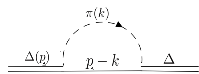
Figure 2: $\pi N$ loop contribution to the $\Delta$ self energy

In the following we will consider only the absorptive (imaginary) parts of the self-energy correction, i.e. we will assume as in Ref.Barbero12 (12) that the parameter $m_{\Delta}$ represents the ’renormalized’ mass of $\Delta$. We place quotation marks as a reminder that the Lagrangian is not renormalizable; only the absorptive corrections are finite in this case. Nevertheless, we have analyzed the effect of the real energy dependent self-energy contribution through dispersive relations and we found that the effect is small Barbero15 (13). If we compute the one-loop absorptive corrections in Fig.(2) by applying the cutting rules, we obtain ($g_{int}=\frac{f_{\pi N\Delta}}{m_{\pi}}$)

$$\Sigma_{\text{abs}}^{\mu\nu}(p_{\Delta})=i\frac{g_{int}^{2}}{2(2\pi)^{2}}\int\frac{d^{3}\text{k}}{2\text{k}_{0}}\frac{1}{2\sqrt{s}}\delta\Bigg{(}\text{k}_{0}+\frac{s+m_{{}_{\pi}}^{2}-m_{{}_{N}}^{2}}{2\sqrt{s}}\Bigg{)}\theta(s-(m_{{}_{N}}+m_{{}_{\pi}})^{2})(\not{p}_{\Delta}+\not{\text{k}}+m_{{}_{N}})\text{k}^{\mu}\text{k}^{\nu},$$ (27)

being $s=p_{\Delta}^{2}$ and when developed in terms of the projectors we can get the corresponding coefficients by solving Eq.(26), and the dressed propagator can be finally obtained (for details see Ref.Barbero12 (12)). Now, we discuss some approximations commonly adopted. If neglected terms of $\mathcal{O}(g_{int}^{3})$ and $\mathcal{O}((m_{\Delta}-\sqrt{s})g_{int}^{2})$ in the dressed propagator expression (see Ref.Barbero15 (13)), since these terms are expected to very small in the in the resonance region $(\sqrt{s}\approx m_{\Delta})$, we get again $G_{0}^{\Delta}$ with the replacement

$$m_{\Delta} \rightarrow m_{\Delta}-i\frac{\Gamma_{{}_{\Delta}}(s)}{2}$$

$$\Gamma_{{}_{\Delta}}(s) = \frac{g_{int}^{2}}{4\pi}\left(\frac{(\sqrt{s}+m_{{}_{N}})^{2}-m_{{}_{\pi}}^{2}}{48s^{5/2}}\right))\lambda^{\frac{3}{2}}(s,m_{{}_{N}}^{2},m_{{}_{\pi}}^{2}),$$ (28)

$$\lambda(x,y,z) = x^{2}+y^{2}+z^{2}-2xy-2xz-2yz.$$

For the sake of completeness, we mention that up to this moment we have considered only the dressing of the Δ propagator. Nevertheless, analyzing the formal scattering T-matrix calculations Mariano07 (11), one can realize that the $\Delta\pi N$ vertex should be also dressed by the rescattering. This of course generates a dependence on $s$ in the vertex, or equivalently an effective coupling constant $g_{int}(s)$, due to the decay in non-resonant amplitudes Mariano07 (11) mediated by the intermediate $\pi N$ propagator.

Now, we consider the formal limit of massless $N$ and $\pi$ in the loop contribution to $\Sigma$ and in the dressed $\pi N\Delta$ vertex, this is the so-called complex-mass scheme (CMS) Amiri92 (14). It assumes within this formal limit that the dressing gives a dependence $g_{int}(s)=\frac{\kappa g_{int}^{0}}{\sqrt{s}}$ ,Barbero15 (13) with $g_{int}^{0}$ being the bare $\pi N\Delta$ coupling constant and $\kappa$ a constant of dimension MeV^-1 to fit, avoiding the direct calculation of the momentum integral in the vertex correction. Thus, we derive from (28) the following approximated expression for the width

$$\Gamma_{\Delta}(s) = \left(1-\frac{\sqrt{s}-m_{\Delta}}{m_{\Delta}}\right)\Gamma_{\Delta}^{CMS},\;\Gamma_{\Delta}^{CMS}=\frac{\kappa^{2}(g_{int}^{0})^{2}}{192\pi}m_{\Delta}.$$ (29)

In the $s\simeq m_{\Delta}^{2}$region we have a constant width $\Gamma_{\Delta}(s)\approx\Gamma_{\Delta}^{CMS}$, where now $\Gamma_{\Delta}^{CMS}$ is fitted in place of $\kappa$ together $g_{int}$ and $m_{\Delta}$ to reproduce $\pi^{+}p$ scattering Mariano01 (20). Note that we have the isospin coefficient in the previous equation equal to 1 for the $\Delta^{++}\rightarrow\pi^{+}p\rightarrow\Delta^{++}$ loop as was shown in the Appendix A. Another approach commonly used, is to fix $\sqrt{s}\approx m_{\Delta}$ in (28) and to use the experimental values for $m_{\Delta}$ and $\Gamma_{\Delta}$ times the branching ratio for the decay into $\pi N$, and get $g_{int}$. We will refer to this as constant mass-width approach (CMW). We will use both the CMS and CMW depending on the considered resonance.

III.1.2 $N^{*}(1520)$ resonance

This $IJ^{\pi}=\frac{1}{2},\frac{3}{2}^{-}$ negative parity resonance has three quark orbital momentum and spin $L=1,S=\frac{1}{2}$. The propagator is (15) but changing $m_{\Delta}\rightarrow m_{1520}$, where we will use the notation $N^{*}(1520)\equiv 1520$. The rescattering in the propagator will be introduced making $m_{{}_{1520}}\rightarrow m_{{}_{1520}}-i\frac{\Gamma_{1520}}{2}$ and since in the second resonance region $W_{\pi N^{\prime}}=\sqrt{(p_{N^{\prime}}+k)^{2}}\lesssim 1600{\text{MeV}}\sim m_{1520}+\Gamma_{1520}$ we can adopt the the CMW with $m_{1520}=1529$ MeV and $\Gamma_{1520}=\Gamma_{1520}^{N\pi}+\Gamma_{1520}^{\Delta\pi}=115$ MeV PTEP20 (15).The strong Lagrangian is given by(Leitner09 (17)):

$$\mathcal{L}_{1520\pi N} = =\frac{f_{{}_{1520\pi N}}}{m_{\pi}}\bar{\Psi}_{\mu}\gamma_{{}_{5}}\partial^{\mu}\bm{\Phi}_{\pi}(x)\cdot\bm{\tau}{\Psi}-\frac{f_{{}_{1520\pi N}}}{m_{\pi}}\bar{\Psi}\partial^{\mu}\bm{\Phi}_{\pi}^{\dagger}(x)\cdot\bm{\tau}\gamma_{5}\Psi_{\mu},$$ (30)

where $\Psi_{\mu}$ is a Rarita - Schwinger field for the spin-$\frac{3}{2}$ but isospin $\frac{1}{2}$. Note that is the same Lagrangian (20) but with $\gamma_{5}$ inserted and changing $\bm{T}\rightarrow\bm{\tau}$ . From this Lagrangian we derive the $N^{*}(1520)\rightarrow\pi N$ vertex decay

$$V^{{}^{1520N\pi}} = \frac{f_{{}_{1520\pi N}}}{m_{\pi}}{\text{k}}_{\mu}\gamma_{{}_{5}}\left(\bm{\Phi}_{\pi}^{{}^{*}}\cdot\bm{\tau}\right),$$

and in Eq.(27) we have a minus sign in the $\not\!p+\not\!k$ term due the $\gamma_{5}$ in the vertex and changing the isospin coefficients to 3 since we have now $\pi^{0}p$ and $\pi^{+}n$ intermediate loop states (see Appendix A), we can get the relation

$$\Sigma_{\text{abs}}^{\mu\nu}(p)(1520) = -\Sigma_{\text{abs}}^{\mu\nu}(p,-m_{\pi,-m_{N)}})(\Delta)$$

this leads to ($g_{int}=\frac{f_{{}_{1520\pi N}}}{m_{\pi}}$)

$$\Gamma_{{}_{1520}}(s) = \frac{3g_{int}^{2}}{4\pi}\left(\frac{(\sqrt{s}-m_{{}_{N}})^{2}-m_{{}_{\pi}}^{2}}{48s^{5/2}}\right)\lambda^{\frac{3}{2}}(s,m_{{}_{N}}^{2},m_{{}_{\pi}}^{2})$$ (31)

$$= \frac{3g_{int}^{2}}{12\pi}\left(\frac{\frac{(\sqrt{s}-m_{{}_{N}})^{2}-m_{{}_{\pi}}^{2}}{2\sqrt{s}}}{\sqrt{s}}\right){\rm q}_{CM}^{3},\;{\rm q}_{CM}=\frac{\lambda^{\frac{3}{2}}(s,m_{{}_{N}}^{2},m_{{}_{\pi}}^{2})}{2\sqrt{s}},$$

that within the CMW the approximation $\sqrt{s}\approx m_{1520}$ it is done and we get the expression used in Ref.(Leitner09 (17)), where $\Gamma_{1520}$ should be weighted by the corresponding $\pi N$ branching ratio decay.

Usually the vector vertex FF for this resonance are expressed in the so called parity conserving parametrization Lakakulich06 (16, 17), nevertheless we want for consistence to express them in the same Sachs parametrization as the other present spin- $\frac{3}{2}$ resonance that is the $\Delta$ . Then, we will assume similar vertex structure than for $\Delta$ in (22) times $\gamma_{5}$ (for the changing in parity), then transform to parity conserving parametrization, compare with Ref.(Leitner09 (17)) and fix our parameters. We get the axial vertex multiplying by $\gamma_{5}$ the $\Delta$ one (25). We get $W^{WN1520}=\left(V^{WN1520}+A^{WN1520}\right)\frac{\sqrt{2}}{2}\left(\bm{W}^{*}\cdot\boldsymbol{\tau}\right)$ with

$$V_{\nu\mu}^{WN1520}(q,p) = \left[(G_{M}(Q^{2})-G_{E}(Q^{2}))K_{\nu\mu}^{M}+G_{E}(Q^{2})K_{\nu\mu}^{E}+G_{C}(Q^{2})K_{\nu\mu}^{C}\right]\gamma_{5},$$ (32)

$$A_{\nu\mu}^{WN1520}(q,p) = i\left[D_{1}(Q^{2})g_{\nu\mu}-\frac{D_{2}(Q^{2})}{m_{{}_{N}}^{2}}(p+p_{1520})^{\alpha}(g_{\mu\nu}q_{\alpha}-q_{\nu}g_{\mu\alpha})+\frac{D_{3}(Q^{2})}{m_{N}^{2}}q_{\mu}p_{\nu}\right]\gamma_{5},$$ (33)

where $K^{i}(q,p)$, $G_{i}(Q^{2})$ and $D_{i}(Q^{2})$ are the same that in Eqs.(22) and (25) but changing $m_{\Delta}\rightarrow m_{1520},p_{\Delta}\rightarrow p_{1520}$, and the values $G_{i}(0),D_{i}(0)$. Note that we have an additional $\frac{1}{2}$ factor coming from the charge operator $\hat{q}=\frac{1+\tau_{3}}{2}$ present in the isospin $\frac{1}{2}$ electromagnetic vertexes but not in the $\frac{3}{2}$ case where we have $T_{3}^{\dagger}$ transition operators.

Now, $V_{\nu\mu}$(we omit super indexes) can be expressed in the so-called “normal parity" (NP) decomposition making use of non-trivial relation

$$-i\epsilon_{\alpha\beta\mu\nu}a^{\mu}b^{\nu}\gamma_{{}_{5}} = (\not{a}\not{b}-a\cdot b)i\sigma_{\alpha\beta}+\not{b}(\gamma_{\alpha}a_{\beta}-\gamma_{\beta}a_{\alpha})-\not{a}(\gamma_{\alpha}b_{\beta}-\gamma_{\beta}b_{\alpha})$$

$$- \not{a}(\gamma_{\alpha}b_{\beta}-\gamma_{\beta}b_{\alpha})+(a_{\alpha}b_{\beta}-a_{\beta}b_{\alpha}),$$

and some on-shell considerations on the resonance, we getting a simplified version of $V_{\nu\mu}$ Barbero15 (13)

$$V_{\nu\mu}(q,p) = i\Bigg{\{}-(G_{M}(Q^{2})-G_{E}(Q^{2}))m_{1520}H_{3\nu\mu}+\Bigg{[}G_{M}(Q^{2})-G_{E}(Q^{2})+2\frac{2G_{E}(Q^{2})(q\cdot p_{1520})-G_{C}(Q^{2})Q^{2}}{(m_{1520}-m_{{}_{N}})^{2}+Q^{2}}\Bigg{]}H_{4\nu\mu}$$ (34)

$$- \Bigg{[}2\frac{2G_{E}(Q^{2})m_{1520}^{2}+(p_{1520}\cdot q)G_{C}(Q^{2})}{(m_{1520}-m_{{}_{N}})^{2}+Q^{2}}\Bigg{]}H_{6\nu\mu}\Bigg{\}}\frac{3(m_{{}_{N}}+m_{1520})}{2m_{{}_{N}}(m_{{}_{N}}+m_{1520})^{2}+Q^{2}},$$

where

$$H_{3}^{\nu\mu}(p,q) = g^{\nu\mu}\not\!q-q^{\nu}\gamma^{\mu},$$

$$H_{4}^{\nu\mu}(p,q) = g^{\nu\mu}q\cdot p_{1520}-q^{\nu}p_{1520}^{\mu},$$

$$H_{5}^{\nu\mu}(p,q) = g^{\nu\mu}q\cdot p-q^{\nu}p^{\nu},$$

$$H_{6}^{\nu\mu}(p,q) = g^{\nu\mu}q^{2}-q^{\nu}p^{\nu}.$$

Note that the $H_{5}^{\nu\mu}$ tensor does not contribute to Eq.(34), but it appears in the general Parity-Conserving expression. The Eq.(32) are independent of taking $p_{1520}=p\mp q$ or $p=p_{1520}\pm q$, (see Eq.(23)) $+$ sign corresponds to the pole contribution and $-$ sign to the cross term. Thus, the Eq(34) is valid in both cases, but the specific value of $q\cdot p_{1520}$ depends on the particular contribution to the amplitudes $\Bigg{(}q\cdot p_{1520}=\pm\frac{m_{{}_{N}}^{2}+Q^{2}-m_{1520}^{2}}{2}\Bigg{)}$. If we set on the $N^{*}(1520)$-pole contribution and replace $p=p_{1520}+q$ we can write Eq. (34) as usually in the parity conserving form

$$V_{\nu\mu}(p,q) = i\Gamma_{\nu\mu}^{V}(p,q),$$

$$\Gamma_{\nu\mu}^{V}(p_{{}_{\text{D}_{13}}},q) = \Bigg{[}-\frac{C_{3}^{V}(Q^{2})}{m_{{}_{N}}}H_{3\nu\mu}-\frac{C_{4}^{V}(Q^{2})}{m_{{}_{N}}^{2}}H_{4\nu\mu}-\frac{C_{5}^{V}(Q^{2})}{m_{{}_{N}}^{2}}H_{5\nu\mu}+\frac{C_{6}^{V}(Q^{2})}{m_{{}_{N}}^{2}}H_{6\nu\mu}\Bigg{]},$$ (35)

where we have the corresponding FF:

$$C_{3}^{V}(Q^{2}) =\frac{m_{1520}}{m_{{}_{N}}}R_{M}\Bigg{[}G_{M}(0)-G_{E}(0)\Bigg{]}F^{V}(Q^{2})$$

$$C_{4}^{V}(Q^{2}) =-R_{M}\Bigg{[}G_{M}(0)-\frac{3m_{1520}}{m_{1520}-m_{{}_{N}}}G_{E}(0)\Bigg{]}F^{V}(Q^{2})$$

$$C_{5}^{V}(Q^{2}) =0$$

$$C_{6}^{V}(Q^{2}) =-R_{M}\frac{2m_{1520}}{m_{1520}-m_{{}_{N}}}G_{E}(0)F^{V}(Q^{2}),$$ (36)

being $R_{M}=\frac{{3}}{{2}}\frac{m_{{}_{N}}}{m_{1520}+m_{{}_{N}}}$ and $F^{V}(Q^{2})=\bigg{(}1+\frac{Q^{2}}{(m_{{}_{N}}+m_{1520})^{2}}\bigg{)}^{-1}G^{V}(Q^{2})$. Note that $\Gamma_{\nu\mu}^{V}(p,q)$ coincides with Eqs.(30) and (31) in Ref. (Leitner09 (17)) making $q\rightarrow-q$ and that now taking the values for $C_{i}^{V}(0)$ from that reference we can get $G_{M,E}(0)$ for the $N^{*}(1520)$ resonance. Rearranging Eq.(33)we get for the pole case

$$A_{\nu\mu}(p,q) = \sqrt{2}i\Bigg{[}\Bigg{(}D_{1}(Q^{2})+\frac{D_{2}(Q^{2})Q^{2}}{m_{{}_{N}}^{2}}\Bigg{)}g_{\nu\mu}-\frac{2D_{2}}{m_{{}_{N}}^{2}}H_{4\nu\mu}+\frac{D_{3}(Q^{2})+D_{2}(Q^{2})}{m_{{}_{N}}^{2}}q_{\nu}q_{\mu}\Bigg{]}\gamma_{5}=i\Gamma_{\mu\nu}^{A},$$

$$\Gamma_{\mu\nu}^{A} =\left[C_{5}^{A}g_{\nu\mu}-\frac{C_{4}^{A}}{m_{{}_{N}}^{2}}g^{\mu\nu}H_{4\nu\mu}+\frac{C_{6}^{A}}{m_{{}_{N}}^{2}}H_{6\mu\nu}\right]\gamma_{5}.$$ (37)

where as before $D_{4}(Q^{2})=0$. Note that this last coincides with Eq.(32) from Ref.Leitner09 (17) making $q\rightarrow-q$. By comparison we get

$$D_{1}+D_{2}\frac{Q^{2}}{m_{{}_{N}}^{2}} = C_{5}^{A},$$

$$-\frac{2D_{2}}{m_{{}_{N}}^{2}} = -\frac{C_{4}^{A}}{m_{{}_{N}}^{2}},$$

$$0 = C_{3}^{A}$$

$$\frac{D_{3}+D_{2}}{m_{{}_{N}}^{2}} = \frac{C_{A}^{6}}{m_{{}_{N}}^{2}}.$$ (38)

From Eqs.(38)one can get from Ref.(Leitner09 (17)) the $D_{i}$ values for the axial resonance $N^{*}(1520)$vertex.

III.2 Spin $\frac{1}{2}$ resonances

For the considered resonances of spin $\frac{1}{2}$ that has three quark orbital momentum and spin $L=0,1,S=\frac{1}{2}$, the parametrization of the hadronic vertex is simpler than for spin- $\frac{3}{2}$ ones and is similar to the parametrization for the $\nu N\rightarrow N^{\prime}$ vertex depending on the parity. We will include the $L=0$, $IJ^{\pi}=\frac{1}{2},\frac{1}{2}^{+}$ $N^{*}(1440)$ resonance and the $L=1$, $IJ^{\pi}=\frac{1}{2},\frac{1}{2}^{-}N^{*}(1535)$ one. The propagator of these resonances looks like the nucleon one but with the replacement $m_{R}\rightarrow m_{R}-i\frac{\Gamma_{R}}{2}$ to introduce the width, and $\Gamma_{R}$ will be considered constant(CMW) since the second resonance region extends to $1600$ MeV and close to the centroids. We get

$$S_{R}(p) = \frac{\not{p}+m_{R}}{p^{2}-m_{R}^{2}+i\Gamma_{R}m_{R}},$$ (39)

where $\Gamma_{R}$ should be weighted by the corresponding $\pi N$ branching ratio decay. The $RN\pi$ strong coupling is described by the Lagrangian Leitner09 (17):

$$\mathcal{L}_{RN\pi}=\frac{f_{{R\pi N}}}{m_{\pi}}\left(\bar{\Psi}_{R}\gamma^{\mu}\Lambda\bm{\tau}\Psi_{N}\right)\cdot\partial_{\mu}\bm{\Phi}_{\pi}(x)+\frac{f_{R\pi N}}{m_{\pi}}\partial_{\mu}\bm{\Phi}_{\pi}^{\dagger}(x)\cdot\left(\bar{\Psi}_{N}\gamma^{\mu}\Lambda\bm{\tau}\Psi_{P_{11}}\right),$$ (40)

where $\Lambda=\gamma_{5},I$ for positive or negative parity. Note that in the $N^{*}(1440)$ case this Lagrangian is similar to the $\mathcal{L}_{NN\pi}$ . From the Lagrangian (40), we can deduce the $R\pi N$ decay vertex

$$V^{R\pi N}=\pi\frac{f_{{}_{R\pi N}}}{m_{\pi}}\Lambda\not{\text{k}}(\bm{\Phi}_{\pi}^{*}\cdot\bm{\tau}).$$ (41)

For the $W\rightarrow NR$ vertex as we have an outgoing boson, make $q\rightarrow-q$ in the hadronic vertex of Ref.(Lakakulich06 (16)), and the vertex can be written as $W^{WNR\lambda}\times\sqrt{2}\bm{\tau}\cdot\bm{W}^{*}$ with

$$W^{WNR\lambda} =-i\frac{1}{2}\Bigg{[}\frac{g_{1V}}{(m_{{}_{R}}+m_{{}_{N}})^{2}}(Q^{2}\gamma^{\lambda}+\not{q}q^{\lambda})\gamma_{5}-\frac{g_{2V}}{(m_{{}_{R}}+m_{{}_{N}})}i\sigma^{\lambda\nu}q_{\nu}\gamma_{5}-g_{1A}\gamma^{\lambda}+\frac{g_{3A}}{m_{{}_{N}}}q^{\lambda}\Bigg{]}\Lambda$$

$$\Lambda =\gamma_{5},I,\mbox{for parity }\pi=\pm 1,$$ (42)

where we note that Eq.(42) is the same as in Ref.(Leitner09 (17)) making $q\rightarrow-q$ but changing $m_{R}+m_{N}\rightarrow 2m_{N}$ and $g_{1V}$, $g_{2V}$, $g_{1A}$, $g_{3A}$ $\rightarrow$ $\mathcal{F}_{1}$, $\mathcal{F}_{2}$, $-\mathcal{F}_{A}$, $-\mathcal{F}_{P}$. We note the similarity of (42) with the same for nucleons which will be shown in the calculations of the background contributions in the next section.

The term with $g_{3A}$ is called pion-pole term and gives de contribution where the W boson decays in a pion which then interacts with the nucleon. This can be obtained replacing the axial contribution $A^{\lambda}$ by $A^{\lambda}+q^{\mu}q.A/(Q^{2}+m_{\pi}^{2})$ (see $g_{3A}(Q^{2})$ below). Then, one assumes that the resonance is on shell and evaluates $\bar{u}_{R}(\not{q}=\not\!p-\not\!p_{R})\Lambda u=\mp\bar{u}_{R}\Lambda(m_{R}\pm m_{N})u$. The FF for the $W\rightarrow NN^{*}$(1440) vertex are obtained from the connection between electromagnetic resonance production and the helicity amplitudes.The helicity amplitudes describe the nucleon-resonances transition depending on the polarization of the incoming photon and the spins of the baryons Lakakulich06 (16). For non-zero $Q^{2}$, data on helicity amplitudes for the $N^{*}$ resonance are available only for the proton Lakakulich06 (16), where it is assumed that the isovector contribution on the neutrino production is given as $g_{i}^{V}=-2g_{i}^{p}$. The PCAC hypothesis allows us to relate the two form factors and fix their axial values at $Q^{2}=0$(Lakakulich06 (16)), we get

$$g_{1V}(Q^{2}) = \frac{g_{1V}(0)\left(b_{1V}ln(1+\frac{Q^{2}}{GeV^{2}})+\frac{1-\pi}{2}\right)}{(1+Q^{2}/M_{V}^{2})^{2}(1+Q^{2}/a_{1V}M_{V}^{2})},\;g_{2V}(Q^{2})=\frac{g_{2V}(0)\left(b_{2V}ln(1+\frac{Q^{2}}{GeV^{2}})-\frac{1+\pi}{2}\right)}{(1+Q^{2}/M_{V}^{2})^{2}}$$

$$g_{1A}(Q^{2}) = \frac{g_{1A}(0)}{(1+Q^{2}/M_{A}^{2})^{2}(1+Q^{2}/3M_{A}^{2})},\;g_{3A}(Q^{2})=\frac{g_{1A}(0)(m_{R}+\pi m_{{}_{N}})}{Q^{2}+m_{\pi}^{2}}m_{N}.$$ (43)

The coupling $g=\frac{f_{R\pi N}}{m_{\pi}}$ can be obtained of the partial decay width ($R\rightarrow\pi N$) according to (Leitner09 (17))

$$\Gamma_{R\rightarrow\pi N} = \frac{3}{4\pi}g^{2}(m_{R}+\pi m_{N})^{2}\left(\frac{\frac{(\sqrt{s}-\pi m_{{}_{N}})^{2}-m_{{}_{\pi}}^{2}}{2\sqrt{s}}}{\sqrt{s}}\right){\rm q}_{CM},\;{\rm q}_{CM}=\frac{\lambda^{\frac{1}{2}}(s,m_{{}_{N}}^{2},m_{{}_{\pi}}^{2})}{2\sqrt{s}},$$ (44)

using the CMW approach mentioned above.

IV Background and resonance amplitudes

Now we built the different components of $\mathcal{O}_{B}$ and $\mathcal{O}_{R}$ from the Lagrangians shown in the Appendix B and those described in the previous section. We get

$$O_{\text{B}}^{\lambda}(p,p^{\prime},q) = O_{\text{BN}}^{\lambda}(p,p^{\prime},q)+O_{\text{BR}}^{\lambda}(p,p^{\prime},q)$$

$$O_{\text{BN}}^{\lambda}(p,p^{\prime},q) = -i\frac{1}{2}\Bigg{[}F_{1}^{V}(Q^{2})\gamma^{\lambda}-i\frac{F_{2}^{V}(Q^{2})}{2m_{{}_{N}}}\sigma^{\lambda\nu}q_{\nu}-F^{A}(Q^{2})\gamma^{\lambda}\gamma_{{}_{5}}\Bigg{]}i\frac{\not\!p^{\prime}+\not\!q+m_{{}_{N}}}{(p^{\prime}+q)^{2}-m_{{}_{N}}}$$ (45)

$$\times \frac{g_{{}_{\pi NN}}}{2m_{{}_{N}}}\gamma_{{}_{5}}(\not\!p-\not\!p^{\prime}-\not\!q)\sqrt{2}\mathcal{T}_{a}(m_{t},m_{t^{\prime}})$$

$$+ \frac{g_{{}_{\pi NN}}}{2m_{{}_{N}}}\gamma_{{}_{5}}(\not\!p-\not\!p^{\prime}-\not\!q)i\frac{\not\!p-\not\!q+m_{{}_{N}}}{(p-q)^{2}-m_{{}_{N}}^{2}}\left(-i\frac{1}{2}\right)\Bigg{[}F_{1}^{V}(Q^{2})\gamma^{\lambda}-i\frac{F_{2}^{V}(Q^{2})}{2m_{{}_{N}}}\sigma^{\lambda\nu}q_{\nu}-F^{A}(Q^{2})\gamma^{\lambda}\gamma_{{}_{5}}\Bigg{]}$$

$$\times \sqrt{2}\mathcal{T}_{b}(m_{t},m_{t^{\prime}})$$

$$- \frac{i}{(p-p^{\prime})^{2}-m_{\pi}^{2}}iF_{1}^{V}(Q^{2})(2p-2p^{\prime}-q)^{\lambda}\times\frac{g_{{}_{\pi NN}}}{2m_{{}_{N}}}\gamma_{{}_{5}}(\not\!p-\not\!p^{\prime})\sqrt{2}\mathcal{T}_{c}(m_{t},m_{t^{\prime}})$$

$$+ \frac{g_{{}_{\pi NN}}}{2m_{{}_{N}}}F_{1}^{V}(Q^{2})\gamma_{{}_{5}}\gamma^{\lambda}\sqrt{2}\mathcal{T}_{d}(m_{t},m_{t^{\prime}})$$

$$+ i\frac{g_{{}_{\omega\pi V}}}{m_{\pi}}F_{1}^{V}(Q^{2})\epsilon^{\lambda\alpha\beta\delta}q_{{}_{\alpha}}(p-p^{\prime})_{{}_{\beta}}i\frac{-g_{{}_{\delta\epsilon}}}{(p-p^{\prime})^{2}-m_{\omega}^{2}}(-i)\frac{g_{{}_{\omega NN}}}{2}\Bigg{[}\gamma^{\epsilon}-i\frac{\kappa_{\omega}}{2m_{{}_{N}}}\sigma^{\epsilon\kappa}(p-p^{\prime})_{\kappa}\Bigg{]}$$

$$\times \sqrt{2}\mathcal{T}_{e}(m_{t},m_{t^{\prime}})$$

$$+ f_{\rho\pi A}F^{A}(Q^{2})i\frac{-g^{\lambda\mu}}{(p-p^{\prime})^{2}-m_{\rho}^{2}}(-i)\frac{g_{{}_{\rho NN}}}{2}\Bigg{[}\gamma_{\mu}-i\frac{\kappa_{\rho}}{2m_{{}_{N}}}\sigma_{\mu\kappa}(p-p^{\prime})^{\kappa}\Bigg{]}\sqrt{2}\mathcal{T}_{f}(m_{t},m_{t^{\prime}}),$$

$$O_{\text{BR}}^{\lambda}(p,p^{\prime},q) =- i\frac{1}{2}\Bigg{[}\frac{g_{1V}^{1440}}{(m_{{}_{1440}}+m_{{}_{N}})^{2}}(Q^{2}\gamma^{\lambda}+\not\!qq^{\lambda})-\frac{g_{2V}^{1440}}{(m_{{}_{1440}}+m_{{}_{N}})}i\sigma^{\lambda\nu}q_{\nu}-g_{1A}^{1440}\gamma^{\lambda}\gamma_{5}+\frac{g_{3A}^{1440}}{m_{{}_{N}}}q^{\lambda}\gamma_{5}\Bigg{]}$$ (46)

$$\times i\frac{\not\!p^{\prime}+\not\!q+m_{R}}{(p^{\prime}+q)^{2}-m_{1440}^{2}+i\Gamma_{1440}m_{1440}}(-)\frac{f_{{}_{1440\pi N}}}{m_{\pi}}\gamma_{5}(\not\!p-\not\!p^{\prime}-\not\!q)\sqrt{2}\mathcal{T}_{g}^{1440}(m_{t},m_{t^{\prime}})$$

$$- i\frac{1}{2}\gamma_{5}\Bigg{[}\frac{g_{1V}^{1535}}{(m_{{}_{1535}}+m_{{}_{N}})^{2}}(Q^{2}\gamma^{\lambda}+\not\!qq^{\lambda})-\frac{g_{2V}^{1535}}{(m_{{}_{1535}}+m_{{}_{N}})}i\sigma^{\lambda\nu}q_{\nu}-g_{1A}^{1535}\gamma^{\lambda}\gamma_{5}+\frac{g_{3A}^{1535}}{m_{{}_{N}}}q^{\lambda}\gamma_{5}\Bigg{]}$$

$$\times i\frac{\not\!p^{\prime}+\not\!q+m_{1535}}{(p^{\prime}+q)^{2}-m_{1535}^{2}+i\Gamma_{1535}m_{1535}}(-)\frac{f_{{}_{1535\pi N}}}{m_{\pi}}(\not\!p-\not\!p^{\prime}-\not\!q)\sqrt{2}\mathcal{T}_{g}^{1535}(m_{t},m_{t^{\prime}})$$

$$+ (-\overline{){W_{\lambda\alpha}^{WN\Delta}(p,p^{\prime},-q)}}iG_{\Delta}^{\alpha\beta}(p^{\prime}+q)(-)\frac{f_{{}_{\pi N\Delta}}}{m_{\pi}}(p-p^{\prime}-q)_{\beta}\sqrt{2}\mathcal{T}_{g}^{\Delta}(m_{t},m_{t^{\prime}})$$

$$+ (-\overline{){\frac{1}{2}W_{\lambda\alpha}^{WN1520}(p,p^{\prime},-q)}}iG_{1520}^{\alpha\beta}(p^{\prime}+q)(-)\frac{f_{{}_{\pi N1520}}}{m_{\pi}}\gamma_{5}(p-p^{\prime}-q)_{\beta}\sqrt{2}\mathcal{T}_{g}^{1520}(m_{t},m_{t^{\prime}}),$$

where the background contributions were splitted in those coming from the nucleon contributions and those coming from the resonances one. Here $\mathcal{T}(m_{t},m_{t^{\prime}})$ are isospin factors calculated between the initial an final nucleon with isospin $m_{t},m_{t}^{\prime}$ projections respectively for each amplitude contribution. Note that the $\frac{1}{2}$ factor in the weak vertex of the isospin $\frac{1}{2}$ resonances comes from the isovector part of the charge operator $\frac{\tau_{3}}{2}$ dragged from the CVC hypothesis. The corresponding pole contributions coming from the resonances are

$$\mathcal{O}_{R}^{\lambda} = \frac{f_{{}_{1440\pi N}}}{m_{\pi}}\gamma_{5}(\not\!p-\not\!p^{\prime}-\not\!q)i\frac{\not\!p-\not\!q+m_{R}}{(p-q)^{2}-m_{1440}^{2}+i\Gamma_{1440}m_{1440}}$$ (47)

$$\times (-i)\frac{1}{2}\Bigg{[}\frac{g_{1V}^{1440}}{(m_{{}_{1440}}+m_{{}_{N}})^{2}}(Q^{2}\gamma^{\lambda}+\not\!qq^{\lambda})-\frac{g_{2V}^{1440}}{(m_{{}_{1440}}+m_{{}_{N}})}i\sigma^{\lambda\nu}q_{\nu}-g_{1A}^{1440}\gamma^{\lambda}\gamma_{5}+\frac{g_{3A}^{1440}}{m_{{}_{N}}}q^{\lambda}\gamma_{5}\Bigg{]}\sqrt{2}\mathcal{T}_{h}^{1440}(m_{t},m_{t^{\prime}})$$

$$+ (-)\frac{f_{{}_{1535\pi N}}}{m_{\pi}}(\not\!p-\not\!p^{\prime}-\not\!q)i\frac{\not\!p-\not\!q+m_{1535}}{(p-q)^{2}-m_{1535}^{2}+i\Gamma_{1535}m_{1535}}$$

$$\times (-i)\frac{1}{2}\Bigg{[}\frac{g_{1V}^{1535}}{(m_{{}_{1535}}+m_{{}_{N}})^{2}}(Q^{2}\gamma^{\lambda}+\not\!qq^{\lambda})-\frac{g_{2V}^{1535}}{(m_{{}_{1535}}+m_{{}_{N}})}i\sigma^{\lambda\nu}q_{\nu}-g_{1A}^{1535}\gamma^{\lambda}\gamma_{5}+\frac{g_{3A}^{1535}}{m_{{}_{N}}}q^{\lambda}\gamma_{5}\Bigg{]}\gamma_{5}\mathcal{T}_{h}^{1335}(m_{t},m_{t^{\prime}})$$

$$+ (-)\frac{f_{{}_{\pi N\Delta}}}{m_{\pi}}(p-p^{\prime}-q)_{\alpha}iG_{\Delta}^{\alpha\beta}(p-q)W_{\beta\lambda}^{WN\Delta}(p,p^{\prime},q)\sqrt{2}\mathcal{T}_{h}^{\Delta}(m_{t},m_{t^{\prime}})$$

$$+ (-)\frac{f_{{}_{\pi N1520}}}{m_{\pi}}\gamma_{5}(p-p^{\prime}-q)_{\alpha}iG_{1520}^{\alpha\beta}(p-q)W_{\beta\lambda}^{WN1520}(p,p^{\prime},q)\sqrt{2}\mathcal{T}_{h}^{1520}(m_{t},m_{t^{\prime}}).$$

Here we show the isospin coefficients calculated with the ingredients of appendix A

$$\mathcal{T}_{a}(m_{t},m_{t^{\prime}}) =\mathcal{T}_{g}^{1440,1535,1520}(m_{t},m_{t^{\prime}})=\chi^{\dagger}(m_{t^{\prime}})({\bm{\tau}\cdot{\bf W^{*}}})({\bm{\tau}\cdot\bm{\Phi}_{\pi}^{*}})\chi(m_{t})=-2,0,-\sqrt{2}$$

$$\mathcal{T}_{b}(m_{t},m_{t^{\prime}}) =\mathcal{T}_{h}^{1440,1535,1520}(m_{t},m_{t^{\prime}})=\chi^{\dagger}(m_{t^{\prime}})({\bm{\tau}\cdot\bm{\Phi}_{\pi}^{*}})({\bm{\tau}\cdot{\bf W^{*}}})\chi(m_{t})=0,-2,\sqrt{2}$$

$$\mathcal{T}_{c}(m_{t},m_{t^{\prime}}) =-i\chi^{\dagger}(m_{t^{\prime}})[({\bm{\Phi}_{\pi}^{*}\times\bm{\Phi}_{\pi^{\prime}}})\cdot{\bf W^{*}}]({\bm{\tau}\cdot}\bm{\Phi}_{\pi^{\prime}}^{*})\chi(m_{t^{\prime}})=1,-1,\sqrt{2}$$

$$\mathcal{T}_{d}(m_{t},m_{t^{\prime}}) =\chi^{\dagger}(m_{t^{\prime}})[(\bm{\Phi}_{\pi}^{*}\times\bm{\tau})\cdot{\bf W^{*}}]\chi(m_{t})=-1,1,-\sqrt{2}$$

$$\mathcal{T}_{e}(m_{t},m_{t^{\prime}}) =\chi^{\dagger}(m_{t^{\prime}})(\bm{\Phi}_{\pi}^{*}\cdot{\bf W^{*}})\chi(m_{t})=-1,-1,0$$

$$\mathcal{T}_{f}(m_{t},m_{t^{\prime}}) =i\chi^{\dagger}(m_{t^{\prime}})[(\bm{\Phi}_{\pi}^{*}\times\bm{\rho})\cdot{\bf W^{*}}](\bm{\tau}\cdot\bm{\rho}^{*})\chi(m_{t})=-1,1,-\sqrt{2}$$

$$\mathcal{T}_{g}^{\Delta}(m_{t},m_{t^{\prime}}) =\chi^{\dagger}(m_{t^{\prime}})({\bf T\cdot W^{*}})({\bf T^{\dagger}}\cdot\bm{\Phi}_{\pi}^{*})\chi(m_{t})=-1/3,\sqrt{2}/3,-1$$

$$\mathcal{T}_{h}^{\Delta}(m_{t},m_{t^{\prime}}) =\chi^{\dagger}(m_{t^{\prime}})({\bf T}\cdot\bm{\Phi}_{\pi}^{*})({\bf T^{\dagger}\cdot W^{*}})\chi(m_{t})=-1,-\sqrt{2}/3,-1/3.$$ (48)

V Form factors and Results

In this work we analyze as a first step the total cross section for the charged current (CC) modes of the six processes

$$\nu p \rightarrow \mu^{-}p\pi^{+},\hskip 11.38092pt\nu n\rightarrow\mu^{-}p\pi^{0},\hskip 11.38092pt\nu n\rightarrow\mu^{-}n\pi^{+},$$

$$\bar{\nu}n \rightarrow \mu^{+}n\pi^{-},\hskip 11.38092pt\bar{\nu}p\rightarrow\mu^{+}p\pi^{-},\hskip 11.38092pt\bar{\nu}p\rightarrow\mu^{+}n\pi^{0},$$ (49)

with $\nu$($\bar{\nu}$) energies exciting the second resonance region and the corresponding cutoffs in $W_{\pi N^{\prime}}$. We will obtain this total cross section through the Eqs.(5-8)with the amplitude (3), taking $(1-\gamma_{5})$ when $\text{$\nu$}\rightarrow\bar{\nu}$, and the vertex production contributions in Eqs.(45-48).

V.1 Parameters and Form Factors

What remains is to define the hadronic FF and the different coupling constants. The coupling constant we use are the values from pion-nucleon scattering, analysis of photo-production and electroproduction of pions. For the strong couplings of nucleons we take $g_{{}_{\pi NN}}^{2}/4\pi=14$,(note that $\frac{f_{\pi NN}}{m_{\pi}}=\frac{g_{\pi NN}}{2m_{N}}$) $g_{{}_{\rho NN}}^{2}/4\pi=2.9$, $\kappa_{\rho}=3.7$, $g_{\omega NN}=3g_{{}_{\rho NN}}$ and $\kappa_{\omega}=-0.12$ Mariano01 (20) with the usually adopted masses for involved hadrons PTEP20 (15, 21). The coupling of nucleon $\rho$ and $\omega$ mesons were obtained by assuming the vector dominance model. In the weak sector the vector coupling constant are fixed by assuming the CVC hypothesis both, for B an R amplitudes. As usual, for the axial currents we exploit the PCAC hypothesis and Golderberg-Treiman relations with exception of the $\Delta$, the most important resonance in this region, where the axial couplings are obtained by fitting to the differential cross section(see below). For the nucleon Born and meson exchange contributions in $\mathcal{O}_{BN}^{\lambda}$ we adopt $g_{{}_{V}}=1$, $g_{{}_{\omega\pi V}}=0.324e$Mariano07 (11), while for the axial couplings we assume $g_{{}_{A}}=1.26$ (PCAC values) and $f_{{}_{\rho\pi A}}=\frac{m_{{}_{\rho}}^{2}}{(93\text{MeV})g_{{}_{\rho NN}}}$ Sato03 (22).

The FF are expressed in terms of the usual Sachs dipole model for the vector current and also a dipole FF for the axial part Barbero08 (10):

$$F_{{}_{1}}^{V}(Q^{2}) =\frac{g_{{}_{V}}}{1+t}\Bigg{[}G_{{}_{E}}^{p}(Q^{2})-G_{{}_{E}}^{n}(Q^{2})+t(G_{{}_{M}}^{p}(Q^{2})-G_{{}_{M}}^{n}(Q^{2}))\Bigg{]},$$

$$F_{{}_{2}}^{V}(Q^{2}) =\frac{g_{{}_{V}}}{1+t}\Bigg{[}G_{{}_{M}}^{p}(Q^{2})-G_{{}_{M}}^{n}(Q^{2})-(G_{{}_{E}}^{p}(Q^{2})-G_{{}_{E}}^{n}(Q^{2}))\Bigg{]},$$

$$F^{A}(Q^{2}) =\frac{g_{{}_{A}}}{(1+Q^{2}/M_{{}_{A}}^{2})^{2}},\hskip 14.22636ptM_{{}_{A}}=1.032\text{ GeV},$$ (50)

where $t=Q^{2}/4m_{{}_{N}}^{2}$ and

$$G_{{}_{E}}^{p}(Q^{2})=\frac{1}{1+\kappa_{{}_{p}}}G_{{}_{M}}^{p}(Q^{2})=\frac{1}{\kappa_{n}}G_{{}_{M}}^{n}(Q^{2})=\frac{1}{1+Q^{2}/M_{{}_{V}}^{2}},\text{\hskip 14.22636pt}G_{{}_{E}}^{n}(Q^{2})=0,$$

with $M_{{}_{V}}^{2}=0.71$ GeV², $\kappa_{{}_{p}}=1.79$, $\kappa_{{}_{n}}=-1.91$. In the case of the contribution involving the $W\pi\pi$ vertex (third term in Eq. 45) we adopt the same $F_{{}_{V}}^{1}(Q^{2})$ as in the other Born terms (first, second and fourth terms in Eq. (45)) since these together should produce a gauge invariant amplitude in the electromagnetic case.

Now, we define parameters and FF for the resonances. We begin with the spin- $\frac{1}{2}$ ones.The coupling $f_{1440\pi N}$ can be obtained from the partial decay width $N^{*}(1440)\rightarrow\pi N$ from Eq.(44) with $\pi=+1,m_{1440}=1462\text{ MeV},\Gamma_{1440}=391\text{ MeV}$PTEP20 (15), making the approach $\sqrt{s}\approx m_{1440}$ (CMW). We take $\Gamma_{{}_{1440\rightarrow\pi N}}\approx 0.69\times 391$ MeV $=269.79$ MeV Leitner09 (17) were the factor $0.69$ comes from the branching ratio of decay in $N\pi$ which is between 55% and 75%. With this width we get the value of $f_{{}_{1440\pi N}}=0.412.$

The weak $W^{WN1440}$ vertex are obtained from the connection between electromagnetic resonance production and the helicity amplitudes.The helicity amplitudes describe the nucleon-resonances transition depending on the polarization of the incoming photon and the spins of the baryons Lakakulich06 (16). For non-zero $Q^{2}$, data on helicity amplitudes for the $N^{*}(1440)$ are available only for the proton Lakakulich06 (16), where it is assumed that the isovector contribution on the neutrino production is given as $g_{i}^{V}=-2g_{i}^{p}$. The PCAC hypothesis allows us to relate the strong and weak FF and fix their values at $Q^{2}=0$. We adopt the following parametrization and values taken from Ref. Lakakulich06 (16)

$$g_{1V}^{1440}(Q^{2})=\frac{4.6}{(1+Q^{2}/M_{V}^{2})^{2}(1+Q^{2}/4.3M_{V}^{2})} g_{2V}^{1440}(Q^{2})=\frac{1.52}{(1+Q^{2}/M_{V}^{2})^{2}}(2.8\ln(1+Q^{2}/\text{GeV}^{2})-1),$$ ,

$$g_{1A}^{1440}(Q^{2}) = \frac{0.51}{(1+Q^{2}/M_{A}^{2})^{2}(1+Q^{2}/3M_{A}^{2})},$$

$$g_{3A}^{1440}(Q^{2}) = 0.51\frac{(m_{1440}+m_{{}_{N}})}{Q^{2}+m_{\pi}^{2}}m_{N},$$ (51)

with $M_{V}=0.84$GeV and $M_{A}=1.05$ GeV. Note that the signs of $g_{1V}(Q^{2}),g_{2V}(Q^{2}),g_{1A}(Q^{2})$ are the same that for $F_{1V}(Q^{2}),F_{2V}(Q^{2}),F_{A}(Q^{2})$ in (50) in spite we have different form factors. For the $N^{*}(1535)$ resonance we get from the same procedure followed before for the $N^{*}(1440)$ using Eq. (44) but for $\pi=-1,m_{1535}=1534\text{ MeV}$, $\Gamma_{1535}=151\text{ MeV}$ and a branching-ratio of 0.51 PDG06 (21) a value $f_{{}_{1535\pi N}}=0.17$, while for the weak FF we get

$$g_{1V}^{1535} =\frac{4.0}{(1+Q^{2}/M_{V}^{2})^{2}(1+Q^{2}/1.2M_{V}^{2})}(7.2\ln(1+Q^{2}/\text{GeV}^{2})+1),$$

$$g_{2V}^{1535} =\frac{1.68}{(1+Q^{2}/M_{V}^{2})^{2}}(0.11\ln(1+Q^{2}/\text{GeV}^{2})),$$

$$g_{1A}^{1535} =\frac{0.21}{(1+Q^{2}/M_{A}^{2})^{2}(1+Q^{2}/3M_{A}^{2})},$$

$$g_{3A}^{1535} =\frac{0.21(m_{1535}-m_{{}_{N}})m_{{}_{N}}}{Q^{2}+m_{\pi}^{2}}.$$ (52)

We analyze now the spin- $\frac{3}{2}$ resonances beginning with the $\Delta$ one. For this resonance, for the mass, width and $\pi N\Delta$ coupling constant we assume consistently the values obtained previously from fitting the $\pi^{{}^{+}}p$ scattering data Barbero08 (10), using the propagator (15) within the CMS approach and the strong vertex (21). We got $f_{{}_{N\pi\Delta}}^{2}/4\pi=0.317\pm 0.003$, $m_{{}_{\Delta}}=1211.7\pm 0.4$ MeV and $\Gamma_{{}_{\Delta}}=92.2\pm 0.4$ MeV. For the vector $\Delta$ weak contribution to the B and R amplitudes we use the effective (empirical) values $G_{{}_{M}}(0)=2.97$, $G_{{}_{E}}(0)=0.055$ and $G_{{}_{C}}(0)=\frac{2m_{{}_{\Delta}}}{m_{{}_{N}}-m_{{}_{\Delta}}}G_{{}_{E}}(0)$ fixed from photo and electroproduction reactions Mariano07 (11, 19). We call these "effective" values, as discussed in Ref. Mariano07 (11), because they correspond to the bare ones $G_{{}_{i}}^{0}(0)$ (usually related with quark models(QM)) renormalized through the decay of a $\pi N$ state coming from the B amplitude into a $\Delta$ through final state interactions (FSI). In Ref. Mariano07 (11) we also get the bare $G_{{}_{E,M}}^{0}(0)$ values by introducing dynamically the FSI by an explicit evaluation of the rescattering amplitudes and showed that the effective values, which are obtained through a fitting procedure, can be in fact interpreted as the "dressed" ones. For the FF we adopt

$$G_{{}_{i}}(Q^{2}) = G_{{}_{i}}(0)(1-Q^{2}/M_{{}_{V}}^{2})^{-2}(1+aQ^{2})e^{-bQ^{2}},$$ (53)

with $a=0.154$/GeV² and $b=0.166$/GeV², for $i=M$, $E$, $C$, which corresponds also to Sachs dipole model times a corrections factor already used in electroproduction calculations Sato1 (19). The axial FF at $Q^{2}=0$, $D_{{}_{i}}(0),$ $i=1,4$, are obtained by comparing the non-relativistic limit of the amplitude $\bar{u}_{{}_{\Delta}}^{\nu}A_{\nu\mu}u$ in the $\Delta$ rest frame ($p_{\Delta}=(m_{{}_{\Delta}},{\bf 0})$, $p=(E_{{}_{N}}({\bf q}),$ $-{\bf q}$) with the non-relativistic QM Sato03 (22, 23). $D_{4}(Q^{2})=0$ since we will not take into account the contribution of the $\Delta$ deformation to the axial current. The $Q^{2}$ dependence of $D_{i}$ is taken to be the same as in vector case with a different parameter in the dipole factor, i.e.

$$D_{{}_{i}}(Q^{2}) = D_{i}(0)F(Q^{2}),\>\mbox{for }i=1,2,\hskip 14.22636pt,D_{3}(Q^{2})=D_{3}(0)F(Q^{2})\frac{m_{{}_{N}}^{2}}{Q^{2}+m_{{}_{\pi}}^{2}},$$ (54)

with $M_{{}_{A}}=1.02$ GeV and $F(Q^{2})=(1+Q^{2}/M_{A}^{2})^{-2}(1+aQ^{2})e^{-bQ^{2}}.$ Here

$$D_{{}_{1}}(0)=\frac{3\sqrt{2}g_{{}_{A}}}{5}\frac{m_{{}_{N}}+m_{{}_{\Delta}}}{2m_{{}_{N}}F(-(m_{{}_{\Delta}}-m_{{}_{N}})^{2})},\,D_{2}(0)=-D_{1}(0)\frac{m_{N}^{2}}{(m_{N}+m_{\Delta})^{2}},\,D_{3}(0)=D_{1}(0)\frac{2m_{N}^{3}}{(m_{N}+m_{\Delta})m_{\pi}^{2}},$$

where $F(-(m_{\Delta}-m_{N})^{2}$) in the denominator comes from the fact that we scale $D_{i}(Q^{2}=-q^{2})$ from the time-like point $q_{0}^{2}=(m_{\Delta}-m_{N})^{2}$ to $q^{2}=0$ through $F(Q^{2})$. Then, as in the case of pion photo-production , we will consider $D_{1}(0)$ as a free (effective or empirical) parameter to be fitted from the experimental data for $d\sigma/dQ^{2}$ and including the FSI effectively. From this fit we get $D_{1}(0)=\frac{2.35}{\sqrt{2}}\mbox{ with }\chi^{2}/dof=0.71$, and results are shown with full lines in the Fig.2 of Ref. Barbero08 (10) where a comparison with the data from the ANL and BNL experiments Rad82 (2, 3) of the neutrino flux $\phi(E_{\nu})$ averaged cross section

$$\left\langle\frac{d\sigma}{dQ^{2}}\right\rangle = \frac{\int\limits_{E_{\nu}^{\text{min}}}^{E_{\nu}^{\text{max}}}\frac{d\sigma({E_{{}_{\nu}}})}{dQ^{2}}\phi(E_{\nu})dE_{\nu}}{\int\limits_{E_{\nu}^{\text{min}}}^{E_{\nu}^{\text{max}}}\phi(E_{\nu})dE_{\nu}},$$

for the main channel $\nu p\longrightarrow\mu^{-}\pi^{+}p^{\prime}$ with the cut $W_{\pi N^{\prime}}<1.4$ GeV in the final invariant mass is done. With this cut it is expected, at less for this channel, that the contributions of more energetic resonances than the $\Delta(1232)$ are small and that are important for more energetic cuts. This will be analyzed in the nect subsection. As the reanalyzed data of ANL achieved in Ref.Rodriguez16 (7) does not affect appreciably the channel used to fit $D_{1}(0)$ for the mentioned cut we do not make a new fitting with $\left\langle\frac{d\sigma}{dQ^{2}}\right\rangle$ nor show again results for this, and we concentrate in the results for the total cross section $\sigma(E_{\nu,\bar{\nu}})$ .

Now we fix parameters, coupling constant and FF for the $N^{*}(1520)$ resonance. From Eq.(31) making the CMW approach $\sqrt{s}\approx m_{1520}=1524$ MeV, $\Gamma_{1520}=115$ MeV and using the partial width $0.55$ PDG06 (21) for decaying into $\pi N$ states we get $\frac{f_{\text{1520$\pi$N}}}{4\pi}=0.2$. Choosing the values reported for the vector couplings for $Q^{2}=0$ in Ref.Leitner09 (17), we have for the vector part using the Eqs.(36)

$$-2.98 =\frac{{3}}{{2}}\frac{1.52}{0.94+1.52}(G_{M}^{1520}-G_{E}^{1520}),$$

$$4.21 =\frac{-{3}}{2}\Bigg{(}G_{M}^{1520}-\frac{4.56}{1.52-0.94}G_{E}^{1520}\Bigg{)}\frac{0.94}{0.94+1.52},$$ (55)

from where we get $G_{M}^{1520}=-2.62$,$G_{E}^{1520}=0.6$, while for $\Delta$ was $G_{{}_{M}}^{\Delta}=2.97,G_{{}_{E}}^{\Delta}=0.055$, being the change in $G_{M}$ consistent with the change of $C_{3}^{V}$ between both resonances (see Ref.(Lakakulich06 (16))). If we use $C^{V}$ values of Ref(Lakakulich06 (16)) we get $G_{M}=-4.67$ and $G_{E}=-0.26$. For the axial couplings using the pole contribution vertex we have using the $C^{A}$ values from Ref.Leitner09 (17)

$$D_{1}(0) =-\frac{2.15}{\sqrt{2}},$$

$$D_{2}(0) =0,$$

$$D_{3}(0) =-\frac{2.15}{\sqrt{2}}\frac{m_{{}_{N}}^{2}}{m_{\pi}^{2}}.$$ (56)

while for $\Delta$ $D_{1}(0)=\frac{2.35}{\sqrt{2}}$, this is consistent also with the change in $C_{A}^{5}$ (Lakakulich06 (16)). The $Q^{2}$ dependence is assumed similar to that in Eqs. (53) and (54).

V.2 Results

We begin discussing a formal issue referred to spin- $\frac{3}{2}$ resonances. It would be useful to put attention in the Eq.(17) where the $\Delta$(also valid for the $N^{*}(1520)$ case) propagator (14) is written expanding the projectors in Eqs.(15) or Eqs.(16).

Note that if we take $A=-\frac{1}{3}$, our choice in previous works Barbero08 (10, 11), then $b(-\frac{1}{3})=2$ in (17) and $\frac{1}{2}(2Z+(1+4Z)A)=\frac{1}{3}Z-\frac{1}{6}$ in (18). At first, one could choose another value for $A$ while the same is taken for the different vertexes coupled to the propagator. On the other hand, if one takes $A=-1$ then $b(-1)=0$ and only the first term of (14), which sometimes is called (Wrongly) on shell $\frac{3}{2}$ projector, contributes. Nevertheless, as can be seen from (15), for a different value of $A$ $\frac{1}{2}$ off-shell propagation always is present. This is not property of the $\frac{3}{2}$ field, also in the massive vector meson propagator we have present an off-shell lower spin 0 component Berme89 (24). As can be seen from the Eq.(17) for our election the propagator has a contribution with a pole at $p^{2}=m_{\Delta}^{2}$ and another that is not singular. When the value $A=-1$ is adopted this last term is not presented, nevertheless an observation regards the vertexes should be done in order.

As was previously mentioned , quite generally in all interaction vertexes we need a contact transformation invariant form proposed in (18), where $Z$ is an arbitrary parameter independent of $A$ that is property of each interaction ( see Eq.(19)). We concentrate for example in the strong $\pi N\Delta$ decay vertex for choosing $Z$, while fix for simplicity the same value for the photo-production and weak production ones as done in previous works Barbero08 (10, 11). Now we point to the question of the true degree of freedom of the spin $\frac{3}{2}$ field, and remember that this is a constrained quantum field theory. Observe that in the free RS Lagrangian in Eqs.(9) and (10), there is no term containing $\dot{\Psi}_{0}$ . So, the equation of motion for it is a true constraint, and $\Psi_{0}$ has no dynamics. It is necessary then that interactions do not change that fact and as it is shown in Badga17 (26) this is fulfilled for the value $Z=\frac{1}{2}$ . The same conclusion was obtained in the original work of Nath Nath71 (27), where through other method the same value was obtained. Then, we adopt this value for our interaction, in resume we use $A=-1/3$ in propagators an vertexes involving the $\Delta$ plus $Z=\frac{1}{2}$ being $\frac{1}{2}(1+4Z)A+Z=0$ and $R_{\alpha}^{\mu}\left(0\right)=g_{\alpha}^{\mu}$ . This selection will be the same for the $N^{*}(1520)$ that is an spin $\frac{3}{2}$ resonance. In spite of this analysis some authors Sato03 (22, 28, 29, 30)try to get both, the simpler versions for $\frac{3}{2}$ propagator using $A=-1$ and a $\pi N\Delta$ vertex with $\frac{1}{2}(1+4Z)A+Z=0$. This can be read in two different manners. First, if they are adopting the same $Z=\frac{1}{2}$ value (generally this is not discussed at all) as us, we could conclude that there is an inconsistence since they are adopting a value $A=-1$ for the propagator while $A=-1/3$ to get $\frac{1}{2}(1+4Z)A+Z=0$, violating the independence of the amplitude with $A$ . Or second, the different choice $Z=-\frac{1}{2}$ is adopted but not mentioned explicitly, and $A=-1$ it is used in both propagator and vertexes. Nevertheless this $Z$ value does not avoid the dynamics of $\Psi_{0}$ in the $\pi N\Delta$ vertex . En each case, model dependencies are introduced.

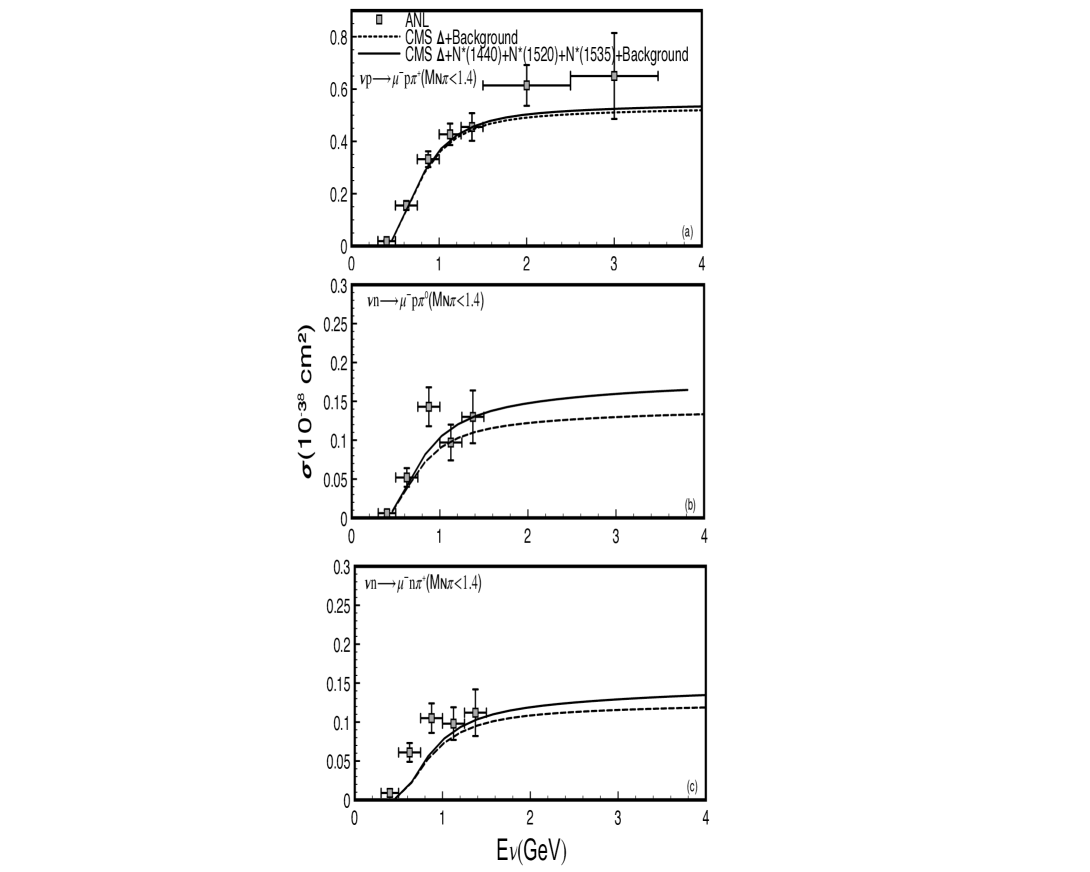
Figure 3: Total $\nu N$ cross section as function of the neutrino energy for different channel. Results with only the $\Delta$ and $\Delta+$ second region resonances plus the corresponding background, in each case are shown for a cut $W_{\pi N}<1.4$ GeV. Data are taken form Ref.Rad82 (2)

In Ref.Barbero08 (10) we have showed the numerical consequences, in the $\Delta$ region, of adopting the value $A=-1$ in the $\Delta$ propagator (called wrongly RS propagator in another works and referred with this name there) keeping inconsistently $A=-1/3$ in the strong and weak $\Delta$ vertexes for the value $Z=1/2$. Results are below the consistent choice results and the data, showing that the inconsistence leads to an observable effect.

Another formal problem is related with the fact that many works do not consider the non-resonant background contributions Lakakulich06 (16) or do not introduce them through the corresponding effective Lagrangians, or do not consider the interference between the background an resonant contributions Lakakulich06 (16, 17) as really it is very important to describe the data. On the other hand, also these models detach the resonance production out of the weak production amplitude Lakakulich06 (16, 17). However, resonances are nonperturbative phenomena associated to the pole of the S-matrix amplitude and one cannot detach them from its production or decay mechanisms, being necessary to built the amplitude through the Feynman rules using the resonance propagators.

Now we show our results. Firstly, in Fig. (3) we compare our calculations without and with the second resonance region included, for $W_{\pi N}<1.4$ GeV for the ANL data (BNL does not give results with this cut for the total cross section). We implement the CMS approach for the $\Delta$ resonance, used previuosly in getting its strong and weak parameters Barbero08 (10, 11, 20), and the CMW for the others. As can be seen the effect of adding more resonances depends on the considered channel. If we considered a fixed energy $E_{\nu}=3,1.5,1.5$ GeV for the mentioned $\nu$ channels in (49) respectively, one can see from the Fig.(3) that their contribution is correspondingly $4\%,17\%$ and $10\%$ , improving the data description regards the model where one includes only the $\Delta$. Note that in spite of the cut in $W_{\pi N}$, the tails of the resonances generated by the finite width give an appreciable contribution and the interference between them is also important.

Analyzing the individual contributions of the $N^{*}(1440),N^{*}(1520),$ and $N^{*}(1535)$ one can notice that the main contribution comes from the $N^{*}(1520)$ being for the other less that $1\%$.
All isospin factors for the mentioned three isospin $\frac{1}{2}$ resonances read

$$\mathcal{T}_{h} = 0,\sqrt{2},-2,\mathcal{T}_{g}=-2,-\sqrt{2},0,$$

and thus this explain why the contribution for the first channel is small since comes from background terms of these resonances. For the second channel we have the main effect since we have contributions of both the direct and cross terms and interference between of them, while for the last one we have only pole contribution. In addition, one could to ask why the contribution of the second resonance region are, apart from the cutting in invariant mass effect, lower than the $\Delta$ + background contributions. This can be understood from the Eqs.(5) and (8) . For certain value of the neutrino energy $E_{\nu}$ in the Lab and $\nu N$ CM systems $E_{\nu}^{CM}\sqrt{s}=E_{\nu}m_{N}$, being the limits in the cross section integrals (6) fixed for a given final $\mu\pi N^{\prime}$ state, and if amplitudes are of the same order of magnitude in the second resonance region regards the $\Delta$ one, the kinetical cross section factor $\frac{1}{E_{\text{$\nu$}}}$ favors smaller neutrinos energies and thus lowest excitation energy contributions. For example if we take the final muon at rest $p_{R}^{2}=(E_{\nu}+m_{N}-m_{\mu})^{2}$ and thus for $p_{\Delta}^{2}=(1232)^{2}$ MeV² we have $\left(m_{N}E_{\nu}\right)^{-1}\approx 2.7$GeV^-2 while for $p_{1520}^{2}=(1520)^{2}$ MeV² we have $\left(m_{N}E_{\nu}\right)^{-1}\approx 1.5$GeV^-2. Then, in spite strong and weak coupling constants would be of the same order the $\Delta$ contribution is favored by the neutrino kinematical factor. This explain the different size of the resonances contribution.

Information about the axial FF $D_{i}(0)$ for the $\Delta$ is carried by the fitting to the differential cross section $d\sigma/dQ^{2}$ data for the cut $W_{\pi N}<1.4$GeVBarbero08 (10) . Therefore, contrasting the model predictions with the ANL and BNL differential data cross sections, will help to complement the model’s quality analysis. Our results for the flux averaged cross sections are shown in Fig. 4, are shown for the $\Delta$ plus background, all resonances plus background both coherent summed in the amplitude and with the incoherent sum of resonant and background cross sections. As can be seen, the efect of adding the second resonance region is noticiable and consistent with the effect on the total cross section in the previous Fig. 3. In addition, it is evident of the effect of adding resonant and backgroud at the amplitud level (coherently) in place at the level of cross section (incoherently).

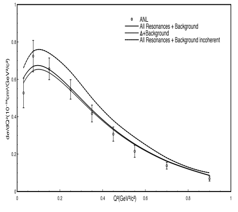
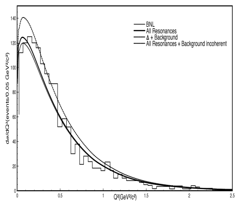
Figure 4: Comparison of the calculated flux averaged differential cross section $d\sigma/dQ^{2}$ for $W_{\pi N}<1.4$GeV with the data of referencies Rad82 (2, 3).

Now we go to the cut $W_{\pi N}<1.6$ GeV where the second resonance region is fully included. As can be seen from the Fig.(5) the contribution of these resonances is more important and necessary to improve the consistence with data. Note that until this moment we keep within the CMS and CMW approaches, the simplest to treat all the resonances togheter the Born terms of the nonresonant background that also include the resonance cross amplitudes.

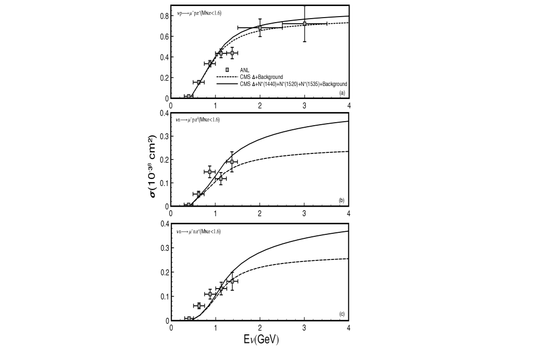
Figure 5: Same as in Figure (3) but for a cut $W_{\pi N}<1.6$ GeV.

Finally we compare the calculated flux averaged cross section $d\sigma/dW_{\pi N}$ for both cuts $1.4$ and $1.6$ GeV with the data for both ANL and BNL experiments in Fig. 6, in order to see with more detail the contribution of the resonant amplitud and background. As can be seen, we have a large background contribution mainly in the $\nu n\rightarrow\mu^{-}\pi^{+}n$ channel, coming for the cross background contribution in Fig. 1(g) for the $\Delta$. This contribution has isospin coefficient $-1$ while the resonant one in Fig. 1(h) has coefficient $-1/3$ giving a small contribution to the cross section when squared. The responsable of this behavior is the second term in the propagator (17) that is present, as consequence of our consistent selection of $A=-1/3,Z=1/2$ and grows for $p^{2}>m_{\Delta}^{2}$ . As this contribution cannot be renormalyzed with a self energy as the pole Fig. 1(h) term, this suggest the neccesity of FF for $W_{\pi N}$ to take into account the finite size of the hadrons not considered in the puntual effective vertexesFeuster98 (31). Of course, in another choices of $A,Z$ where $b(A)=0$ in (17) this growing is not present but the treatment is not consistent. In addition, is not clear that we can extend the another tree non-resonant background contributions in Figs.1(a) to (f) to any final $W_{\pi N}$ keeping structureless hadrons. Finally, it is visible the contribution of the $N^{*}(1520)$ resonance for the $\nu n\rightarrow\mu^{-}\pi^{+}n$ channel due to the value of the isopin factor 2 in this case.

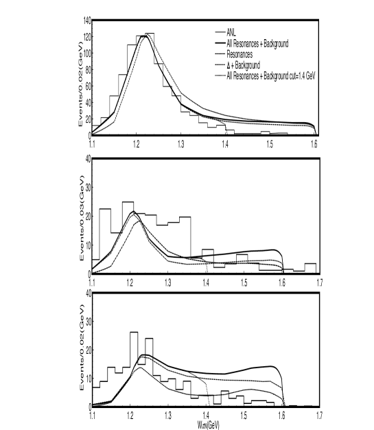
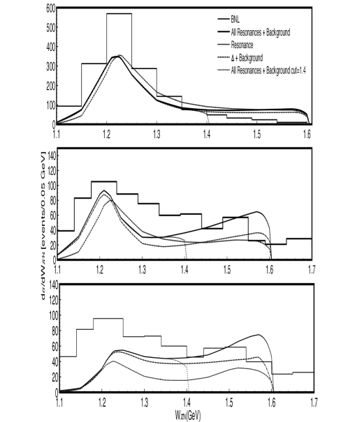
Figure 6: Comparison of the flux averaged $d\sigma/dW_{\pi N}$ cross section with the ANL and BNL data. The values of $W_{\pi N}$ for which theoretical cross section is reported, correspond to the bin’s central values of the ANL or BNL data.

Now, in order to follow probing our model we wish to calculate the antineutrinos total cross sections. We have two differences regards the neutrinos case. Firstly, the interactions of neutrinos with hadrons is not the same that for antineutrinos. We have a sign of difference in the lepton current contraction that makes a different coupling with the hadron one. Then, the interaction with neutrinos is different from antineutrinos due the use of spinors for antiparticles in (3) and has nothing to do with the very know CP violation effect. Secondly, in the experiment we have an admixture of heavy freon CF3Br and was exposed to the CERN PS antineutrino beam (peaked at $E_{\bar{\nu}}\sim$ 1.5 GeV)Bolog79 (25). In this case the experiment informs that we have 0.44% on neutrons and 0.55% of protons, and since our calculations were for free nucleons we weight out results with these percentages depending on the channel $\bar{\nu}n\rightarrow\mu^{+}n\pi^{-}$ or $\bar{\nu}p\rightarrow\mu^{+}np\pi^{-}$. Our results including all resonances and compared with the data are shown in Fig.(7) for the only cut $W_{\pi N}<1.4$ GeV reported inBolog79 (25) , and as can be seen we get a consistent description with the same cut for the neutrino case.

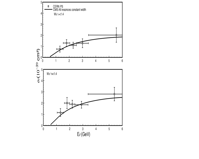
Figure 7: Antineutrino’s total cross sections with a cut in $1.4$ GeV for the $\bar{\nu}n\rightarrow\mu^{+}n\pi^{-}$ and that leading to a final $N\pi^{-}$final state.

Now we analyze the quality of our results and compare with other calculations including the second resonance region, taking into account the formal shortcomings mentioned above. As can be seen from a general point of view, our model that fulfill consistence regards contact transformations in the spin-$\frac{3}{2}$ field reproduce better the ANL data than other inconsistent models Rafi16 (29). In addition, in that reference it seems that the cross resonance contributions are omitted for the $\nu p\rightarrow\mu^{-}\pi^{+}p$ channel. It is true that the direct or pole contribution of isospin- $\frac{1}{2}$ resonances cannot contribute to a isospin-$\frac{3}{2}$ amplitude, but the cross terms do contribute noticing the isospin factors for this channel are not zero in Eq.(48). This make the difference between the full thin lines and the dashed ones in the upper panel of Figs.(3) and (5). A last shortcoming to mention is that for non resonant backgrounds contributions Figs 1(a)-(f), an arbitrary cutoff of $W_{\pi N}<1.2$ GeV is applied changing artificially the behavior of these contributions independently from the rest of terms. This is done for all the presented regimes $W_{\pi N}<1.4,1.6$ GeV. Note that we can reproduce very well these data without the necessity of any special cuttings, all contributions are calculated with the same $W_{\pi N}$ maximum value.
Finally, we note that in Ref.Rafi16 (29) the antineutrino results are not reproduced, while within our model the accordance with the data is very well in all the energy region where the data is reported.

On the other hand, the model adopted in Ref.(Lakakulich06 (16)) where the propagation of the resonance is described by a Breit-Wigner distribution separating production and decay, does not include a background amplitude and to get accordance in the data for the $\nu n\rightarrow\mu^{-}n\pi^{+},\hskip 11.38092pt\nu n\rightarrow\mu^{-}p\pi^{0}$ processes they needed to add incoherently a spin $\frac{1}{2}$ background. The model adopted in Ref.(Leitner09 (17)) is similar to that in (Lakakulich06 (16)) but they adjust the background cross section contribution through a parameter $b^{\pi N}$ different for each channel. These two last works were improved in Ref.Lala10 (30), where the R and B contributions were added coherently and the $\Delta$ propagation is treated with the choice $A=-1,Z=-1/2$ mentioned above, within the parity conserving parametrization of the $WN\rightarrow\Delta$ vertex. These differences make difficult to compare with our results when $R=\Delta$ since we choose a different $A,Z$ choice and the Sachs parametrization.

VI Conclusions

In this work we calculate the pion production cross section including in the model spin- $\frac{1}{2}$ and $\frac{3}{2}$ resonances $\Delta(1232),N^{*}(1440),N^{*}(1520)$ and $N^{*}(1535)$ to cover the so called second resonance region. From the formal point of view the spin- $\frac{3}{2}$ Lagrangians ( free and interaction) respect invariance under contact transformations and the associated parameter $A$, is fixed to be the same in all components of the Feynman rules to get $A$-independent amplitudes. Also, the additional $Z$ parameter present in the $\mathcal{L}_{\pi NR}$ Lagrangian for these resonances is fixed to avoid time evolution of the field component $\Psi_{0}$, since $\dot{\Psi}_{0}$ is not present in the free Lagrangian. It is shown how another models do not analyze these formal facts that can produced model dependence.

We treat the spin- $\frac{1}{2}$ resonances within the parity conserving parametrization for the FF, since this is compatible to that used in the similar topological nucleon contribution in Fig.1 (a) and (b). For the spin- $\frac{3}{2}$ resonances we adopt the Sachs parametrization to be consistent with our previous works including only the $\Delta$ resonance where we get better results than using the parity conserving one Barbero14 (18). We followed the connection between both parameterizations achieved in that reference to get the FF for the $N^{*}(1520)$ resonance and have taken the $Q^{2}$ FF from Ref.(Lakakulich06 (16)) for all the second region resonances. We note that the main contribution comes from the $\Delta$ resonance and the presence of the additional resonances do not change appreciably the results of the cross section for the $\nu p\rightarrow\mu^{-}p\pi^{+}$ channel for the cut $W_{\pi N}<1.4$ GeV as can be seen from Fig.(3). As this cut was used to fix $G_{M}(0),G_{E}(0)$ and $D_{1}(0)$ for the $\Delta$ we keep the same values obtained previously in Refs.(Barbero08 (10, 11)). Firstly, we achieve the comparison with the data of ANL experiment in the region of $W_{\pi N}<1.4,1.6$ GeV, where we have worked within the CMS+CMW approach. From the results including and not including the second resonance region, we conclude that to improve the data, this resonance region should be included. More, in the case $W_{\pi N}<1.4$ GeV one can think why ? We conclude this second energy region is necessary due to the tail of the resonances that have their centroids out of this region, but influences through the tails that interfere between resonance and background contributions. This behavior is confirmed when we compare with the data with the $W_{\pi N}<1.6$ GeV and the good agreement with the data for the antineutrino case. In other approaches as in Ref.Hernandez17 (32) , the replacement ${\cal L}_{\pi N\Delta}\rightarrow{\cal L}_{\pi N\Delta}+c{\cal L}_{C}$ is proposed, with ${\cal L}_{C}$ describing contact terms without the $\Delta$ field, with adjusting the low-energy constant c to get a better fitting for the $\nu n\rightarrow\mu^{-}n\pi^{+}$channel. The addition of contact terms is based on the argumentation that within the ChPT framework, the equivalence between different Lagrangians is at less of low energy constants, to be adjusted. We see that this is not necessary if one includes consistently the second resonance region.

Finally the data of Ref.(Rad82 (2)) contains also results without energy cuts and also all results in Ref.Kitagi86 (3) are reported without events exclusion. In addition a reanalysis of these two set of data has been done recently in Ref.Rodriguez16 (7) where the main results are shown without cuts. For describing them we need to extend the model to higher energies. This will be done in a next contribution.

VII APPENDIX

VII.1 Spin projectors and isospin operators

We have introduced $P_{ij}^{k}$ which projects on the $k=\frac{3}{2}$, $\frac{1}{2}$ sector of the representation space, with $i,j=1,2$ indicating the sub-sectors of the $\frac{1}{2}$ subspace, and are defined as

$$(P^{\frac{3}{2}})_{\mu\nu} = g_{\mu\nu}-\frac{1}{3}\gamma_{\mu}\gamma_{\nu}-\frac{1}{3p^{2}}\left[\not\!p\gamma_{\mu}p_{\nu}+p_{\mu}\gamma_{\nu}\not\!p\right],$$

$$(P_{22}^{\frac{1}{2}})_{\mu\nu} = \frac{p_{\mu}p_{\nu}}{p^{2}},$$

$$(P_{11}^{\frac{1}{2}})_{\mu\nu} = g_{\mu\nu}-P_{\mu\nu}^{\frac{3}{2}}-(P_{22}^{\frac{1}{2}})_{\mu\nu}$$

$$= (g_{\mu\alpha}-\frac{p_{\mu}p_{\alpha}}{p^{2}})(1/3\gamma^{\alpha}\gamma^{\beta})(g_{\beta\nu}-\frac{p_{\beta}p_{\nu}}{p^{2}}),$$

$$(P_{12}^{\frac{1}{2}})_{\mu\nu} = \frac{1}{\sqrt{3}p^{2}}(p_{\mu}p_{\nu}-\not\!p\gamma_{\mu}p_{\nu}),$$

$$(P_{21}^{1/2})_{\mu\nu} = \frac{1}{\sqrt{3}p^{2}}(-p_{\mu}p_{\nu}+\not\!pp_{\mu}\gamma_{\nu}).$$ (57)

On the other hand we define the isospin $\Delta$ excitation operators

$$\boldsymbol{T}^{\dagger}\cdot\boldsymbol{\phi}_{+,-,0} = \left(\begin{array}[]{cc}1&0\\ 0&\frac{1}{\sqrt{3}}\\ 0&0\\ 0&1\end{array}\right),\left(\begin{array}[]{cc}0&0\\ 0&0\\ -\frac{1}{\sqrt{3}}&0\\ 0&1\end{array}\right),\left(\begin{array}[]{cc}0&0\\ \sqrt{\frac{2}{3}}&0\\ 0&\sqrt{\frac{2}{3}}\\ 0&0\end{array}\right),$$

that acts on $N=\left(\begin{array}[]{c}1\\ 0\end{array}\right),\left(\begin{array}[]{c}0\\ 1\end{array}\right)$ for proton and neutron respectively and

$$\Delta_{++,+,0,-} = \left(\begin{array}[]{c}1\\ 0\\ 0\\ 0\end{array}\right),\left(\begin{array}[]{c}0\\ 1\\ 0\\ 0\end{array}\right),\left(\begin{array}[]{c}0\\ 0\\ 1\\ 0\end{array}\right),\left(\begin{array}[]{c}0\\ 0\\ 0\\ 1\end{array}\right)$$

for the $\Delta$ states, being $\boldsymbol{\phi}{}_{+,-,0}=\frac{-1}{\sqrt{2}}(1,i,0),\frac{1}{\sqrt{2}}(1,-i,0),(0,0,1)$ and $\boldsymbol{W}_{\pm}=\boldsymbol{\phi}_{\pm}$.
The isospin factors included in the resonances width are for isospin $I=\frac{3}{2},\frac{1}{2}$

$$\Delta_{++}^{\dagger}\left(\boldsymbol{T}^{\dagger}\cdot\boldsymbol{\phi}_{+}\right)\left(\boldsymbol{T}\cdot\boldsymbol{\phi}_{+}^{\dagger}\right)\Delta_{++}=\Delta_{+}^{\dagger}\left[\left(\boldsymbol{T}^{\dagger}\cdot\boldsymbol{\phi}_{+}\right)\left(\boldsymbol{T}\cdot\boldsymbol{\phi}_{+}^{\dagger}\right)+\left(\boldsymbol{T}^{\dagger}\cdot\boldsymbol{\phi}_{0}\right)\left(\boldsymbol{T}\cdot\boldsymbol{\phi}_{0}^{\dagger}\right)\Delta_{+}\right] =\cdots =1$$

$$R^{\dagger}(\frac{1}{2})\left[\left(\tau\cdot\boldsymbol{\phi}_{0}\right)\left(\boldsymbol{\tau}\cdot\boldsymbol{\phi}_{0}^{\dagger}\right)+\left(\tau\cdot\boldsymbol{\phi}_{+}\right)\left(\boldsymbol{\tau}\cdot\boldsymbol{\phi}_{+}^{\dagger}\right)\right]R(\frac{1}{2}) = \cdots=3,$$

since we can have $\pi^{0}p,\pi^{+}n,$ states when we have an isospin $\frac{1}{2}$ projection ($q=e)$ and also $\pi^{0}n,\pi^{-}p$ when isospin projection is $-\frac{1}{2}$ ($q=-e$) or $\pi^{-}n$ only in the $I=3/2$ one with projection $-\frac{3}{2}$.

VII.2 Lagrangians and propagators involved in the non resonant background

The propagators and interaction Lagrangians used to built amplitudes $\mathcal{O}_{BN}$will be resumed here. First the propagators, which come from the inversion of the kinetic operators present in the free Lagrangians are

$$S(p) = \frac{\not\!p+m_{N}}{p^{2}-m^{2}},\>\mbox{{nucleon}}$$

$$\Delta(p) = \frac{1}{p^{2}-m_{\pi}^{2}},\>\mbox{{pion}}$$

$$D_{\mu\nu}(p) = \frac{-g_{\mu\nu}+\frac{p_{\mu}p_{\nu}}{m_{V}^{2}}}{p^{2}-m_{V}^{2}},\>\mbox{{vector-meson}},$$

while the effective strong interacting Lagrangians are

$$\mathscr{L}_{\pi NN}(x) = -\frac{g_{\pi NN}}{2m_{N}}\bar{\psi}(x)\gamma_{5}\gamma_{\mu}\boldsymbol{\tau}\cdot\left(\partial^{\mu}\boldsymbol{\boldsymbol{\phi}}(x)\right)\psi(x),$$

$$\mathscr{L}_{VNN}(x) = -\frac{g_{{}_{V}}}{2}\bar{\psi}(x)\left[\gamma_{\mu}\left\{\begin{array}[]{c}\boldsymbol{\rho}^{\mu}(x)\cdot\boldsymbol{\tau}\\ \omega^{\mu}(x)\end{array}\right\}-\frac{\kappa_{V}}{2m_{N}}\sigma_{\mu\nu}\left(\partial^{\nu}\left\{\begin{array}[]{c}\boldsymbol{\rho}^{\mu}(x)\cdot\boldsymbol{\tau}\\ \omega^{\mu}(x)\end{array}\right\}\right)\right]\psi(x),$$

With $V=\omega,\rho$. Now, we define the effective hadron weak Lagrangians built from Eqs.(1,2)

$$\mathscr{L}_{WNN}(x) = -\frac{g}{2\sqrt{2}}\overline{\psi}(x)\left[\gamma_{\mu}F_{1}^{V}(Q^{2})-\frac{F_{2}^{V}(Q^{2})}{2m_{N}}\sigma_{\mu\nu}\partial^{\nu}-F^{A}(Q^{2})\gamma_{\mu}\gamma_{5}\right]\sqrt{2}\boldsymbol{W}^{\mu}(x)\cdot\frac{\boldsymbol{\tau}}{2}\psi(x)+hc.,$$

$$\mathscr{L}_{W\pi\pi}(x) = -\frac{g}{2\sqrt{2}}F_{1}^{V}(Q^{2})\sqrt{2}\left[\boldsymbol{\boldsymbol{\phi}}(x)\times\partial_{\mu}\boldsymbol{\boldsymbol{\phi}}(x)\right]\cdot\boldsymbol{W}^{\mu}(x),$$

$$\mathscr{L}_{W\pi NN}(x) = -\frac{g}{2\sqrt{2}}\frac{f_{\pi NN}}{m_{\pi}}F_{1}^{V}(Q^{2})\bar{\psi}(x)\gamma_{5}\gamma_{\mu}\sqrt{2}(\boldsymbol{\tau}\times\boldsymbol{\boldsymbol{\phi}}(x))\cdot\boldsymbol{W}^{\mu}\psi(x),$$

$$\mathscr{L}_{W\pi\rho}(x) = \frac{g}{2\sqrt{2}}f_{\rho\pi A}F^{A}(Q^{2})\sqrt{2}\left(\boldsymbol{\boldsymbol{\phi}}(x)\times\boldsymbol{\rho}_{\mu}(x)\right)\cdot\boldsymbol{W}(x)^{\mu}$$

$$\mathscr{L}_{W\pi\omega}(x) = -\frac{g}{2\sqrt{2}}\frac{g_{\omega\pi V}}{m_{\omega}}F_{1}^{V}(Q^{2})\epsilon_{\mu\alpha\lambda\nu}\left(\partial^{\lambda}\boldsymbol{\boldsymbol{\phi}}(x)\right)\cdot\left(\partial^{\mu}\boldsymbol{W}{}^{\alpha}(x)\right)\omega^{\nu}(x).$$

VIII Acknowledgments

A. Mariano, belong to CONICET and UNLP, D.F. Tamayo Agudelo and D.E Jaramillo Arango to UdeA.

References

- (1) C. H. Llewellyn Smith,Phys. Rep., 3, 261, (1972).
- (2) G. M. Radecky, et. al, Phys. Rev. D 25, 1161 (1982).
- (3) T. Kitagaki,et al., Phys. Rev. D 34 , 2554 (1986).
- (4) K.Graczyk,D.Kielczewska,P.Przewlocki,J.Sobczyk,Phys.Rev. D 80, 093001 (2009). doi:10.1103/PhysRevD.80.093001
- (5) K.M. Graczyk, J. Zmuda, J.T. Sobczyk, Phys. Rev. D 90, 093001 (2014). doi:10.1103/PhysRevD.90.093001
- (6) C. Wilkinson, P. Rodrigues, S. Cartwright, L. Thompson, K. McFarland, Phys. Rev. D 90(11), 112017 (2014). doi:10.1103/ Phy
- (7) Philip Rodrigues, Callum Wilkinson,and ,Kevin McFarland, Eur. Phys. J. C (2016) 76:474.
- (8) M. Kirchbach and D. Ahluwalia, Phys.Lett.B, (2002) 529124.
- (9) W. Rarita and J. Schwinger Phys. Rev. 60, 61 (1941).
- (10) C. Barbero, A. Mariano, G. Lopez Castro. Physics letters B 664 (2008) 70-77.
- (11) A. Mariano. Phys. lett. B (2007) 253; A. Mariano, J. Phys. G (2007) 1627.
- (12) C. Barbero, A. Mariano and G. Lï¿œpez Castro, J. Phys. G: Nucl. Part. Phys. 39 (2012) 085011.
- (13) C. Barbero, A. Mariano, J. Phys. G: Nucl. Part. Phys. 42 (2015) 105104 .
- (14) M. el Amiri, J. Pestieau and G. Lṕez Castro, Nucl. Phys. A 543( 1992) 673.
- (15) P.A. Zyla et al. (Particle Data Group), Prog. Theor. Exp. Phys. 2020, (2020)083C01.
- (16) O. Lalakulich, E. A. Paschos, and G. Piranishvili, Phys. Rev. D 74,(2006), 014009 .
- (17) T. Leitner, O. Buss, L. Alvarez-Ruso, and U. Mosel, Phys. Rev. C 79,(2009).
- (18) C. Barbero, A. Mariano, G. Lopez Castro. Physics Letters B 728 (2014) 282-287.
- (19) T. Sato, T-S.H Lee, Phys. Rev. C 63 (2001) 055201.
- (20) G. Lopez Castro, A. Mariano, Nucl. Phys. A 697 (2001)440.
- (21) Review of Particle Physics,W.-M. Yao, et al, J. Phys. G 33 (2006) 1.
- (22) T. Sato, D. Uno, T.-S.H Lee, Phys. Rev. C 67 (2003) 065201.
- (23) T. R. Hemmert, B.R Holstein, Phys. Rev. D 51 (1995) 158.
- (24) M. Bermerrouche, R. M. Davidson, and N. C. Mukhopadhyay, Phys. Rev. C 39, 2339 (1989).
- (25) T. Bolognese, J.P. engel, J.L Guyonnet and J.L. Riester, Phys. Lett. 81B (1979),393.
- (26) D. Badagnani, A. Mariano, and C. Barbero, J. Phys. G: Nucl. Part. Phys. 44, 025001 (2017).
- (27) Nath L M, Etemadi B and Kimel J D 1971 Phys. Rev. D 3 2153.
- (28) E. Hernandez, J. Nieves, M. Valverde, Phys. Rev. D 76, 033005 (2007). doi:10.1103/PhysRevD.76.033005
- (29) M. Rafi Alam, M. Sajjad Athar, S. Chauhan and S. K. SinghInternational Journal of Modern Physics E Vol. 25, No. 2 (2016) 1650010 .
- (30) O. Lalakulich, T. Leitner, O. Buss, and U. Mosel, Phys. Rev. D 82, 093001 (2010)
- (31) T. Feuster and U. Mosel, Phys. Rev. C 58, 457 (1998).
- (32) E. Hernandez and J. Nieves, Phys. Rev. D 95, 053007 (2017).