Coarsening the Granularity: Towards Structurally Sparse Lottery Tickets

Abstract

The lottery ticket hypothesis (LTH) has shown that dense models contain highly sparse subnetworks (i.e., winning tickets) that can be trained in isolation to match full accuracy. Despite many exciting efforts being made, there is one “commonsense” rarely challenged: a winning ticket is found by iterative magnitude pruning (IMP) and hence the resultant pruned subnetworks have only unstructured sparsity. That gap limits the appeal of winning tickets in practice, since the highly irregular sparse patterns are challenging to accelerate on hardware. Meanwhile, directly substituting structured pruning for unstructured pruning in IMP damages performance more severely and is usually unable to locate winning tickets. In this paper, we demonstrate the first positive result that a structurally sparse winning ticket can be effectively found in general. The core idea is to append “post-processing techniques” after each round of (unstructured) IMP, to enforce the formation of structural sparsity. Specifically, we first “re-fill” pruned elements back in some channels deemed to be important, and then “re-group” non-zero elements to create flexible group-wise structural patterns. Both our identified channel- and group-wise structural subnetworks win the lottery, with substantial inference speedups readily supported by existing hardware. Extensive experiments, conducted on diverse datasets across multiple network backbones, consistently validate our proposal, showing that the hardware acceleration roadblock of LTH is now removed. Specifically, the structural winning tickets obtain up to $\{64.93\%,64.84\%,60.23\%\}$ running time savings at $\{36\%\sim 80\%,74\%,58\%\}$ sparsity on {CIFAR, Tiny-ImageNet, ImageNet}, while maintaining comparable accuracy. Code is at https://github.com/VITA-Group/Structure-LTH.

1 Introduction

Recently, the machine learning research community has devoted considerable efforts and financial outlay to scaling deep neural networks (DNNs) to enormous sizes ($175$ billion parameter-counts in GPT-3 (Brown et al., 2020)). Although such overparameterization simplifies the training of DNNs and dramatically improves their generalization (Bartlett et al., 2021; Du et al., 2018; Kaplan et al., 2020), it may severely obstruct the practical usage on resource-limited platforms like mobile devices, due to its large memory footprint and inference time (Hoefler et al., 2021). Pruning is one of the effective remedies that can be dated back to LeCun et al. (1990): it can eliminate substantial redundant model parameters and boost the computational and storage efficiency of DNNs.

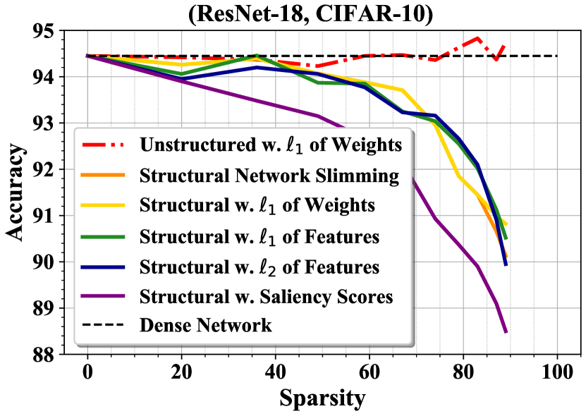
Figure 1: Achieved test accuracy over different sparsity levels of diverse unstructured and structural subnetworks. Sparse models from classical channel-wise structural pruning algorithms (He et al., 2017; Liu et al., 2017; Bartoldson et al., 2019; Molchanov et al., 2019) can not match the full accuracy of the dense model.

Such benefits drive numerous interests in designing model pruning algorithms (Han et al., 2015a, b; Ren et al., 2018; He et al., 2017; Liu et al., 2017). Among this huge family, an emerging representative studies the prospect of training sparse subnetworks in lieu of the full dense models without impacting performance (Frankle & Carbin, 2019; Chen et al., 2020b). For instance, Frankle & Carbin (2019) demonstrates that dense models contain sparse, matching subnetworks (Frankle et al., 2020a) (a.k.a. winning tickets) capable of training in isolation from the original initialization to match or even surpass the full accuracy. This phenomenon is referred to as the lottery tickets hypothesis (LTH), which indicates several impressive observations: $(i)$ usually extreme sparsity levels (e.g., $90\%$, $95\%$) can be achieved without sacrificing the test accuracy; $(ii)$ the located winning ticket maintains undamaged expressive power as its dense counterpart, and can be easily trained from scratch or early-epoch weights (Renda et al., 2020; Frankle et al., 2020a) to recover the full performance. These advances are positive signs of the substantial potential of sparse DNNs.

However, almost all LTH literature investigates unstructured sparsity only. In practical scenarios, it brings little hardware efficiency benefits due to the poor data locality and low parallelism (He et al., 2017; Mao et al., 2017; Wen et al., 2016) caused by highly irregular sparse patterns. Meanwhile, most of the accelerators are optimized for dense matrix operations (Han et al., 2016), which means there is limited speedup for unstructured pruned subnetworks even if the sparsity level exceeds $95\%$ (Wen et al., 2016). Structural pruning (He et al., 2017; Liu et al., 2017) as an alternative to exploring sparse subnetworks, removes the entire filter or channel in DNNs to gain more computational efficiency at the cost of (more) accuracy degradation. As shown in Fig. 1, traditional channel-wise structural pruning approaches (He et al., 2017; Bartoldson et al., 2019; Molchanov et al., 2019) quickly degrade performance and cannot lead to winning tickets, which was also echoed in You et al. (2020).

In our paper, we present the first study into the structural lottery tickets, which explores hardware-friendly structural sparsity (including channel-wise and group-wise patterns) in order to find lottery tickets. Specifically, we start from unstructured sparse subnetworks, and then adopt proposed refilling techniques to create channel-wise structural sparsity by growing back the pruned elements within the most important channels and abandoning the rest. Our results (Section 4) show such refined channel-wise structural subnetworks win the lottery at a moderate sparsity level with $\sim 50\%$ running time savings on an Nvidia 2080 TI GPU. In order to push the compression ratio higher, we introduce a regrouping algorithm based on hypergraph partitioning (Rumi et al., 2020) to establish group-wise structural patterns which are more amenable to pruning due to the shape flexibility of grouped dense blocks. These group-wise structural winning tickets achieve $\sim 60\%$ running time savings at $50\%\sim 80\%$ sparsity without any performance degradation compared to the dense models.

Note that this paper focuses on general structural sparse patterns capable of acceleration, including conventional channel-wise sparsity and other fine-grained structural sparsity. The latter actually becomes prevailing recently since it achieves superior performance and maintains satisfied speedup, sparking great interest in industries such as NVIDIA (N:M) (Zhou et al., 2021) and Google (Block-wise) (Shangguan et al., 2019). Meanwhile, unlike Zhou et al. (2021), our group-wise sparse patterns do NOT need any specific hardware accelerators and are generally applicable to common GPU devices. Lastly, although we mainly investigate inference efficiency, our proposals can also enable efficient training in transfer learning paradigms as demonstrated in Appendix A2. Our main contributions lie in the following aspects:

• To our best knowledge, we are the first to demonstrate the existence of structurally sparse winning tickets at non-trivial sparsity levels (i.e., $>30\%$), and with both channel-wise and group-wise sparse patterns.

• We propose the refilling technique and introduce the regrouping algorithm to form channel-wise and group-wise structural sparsity. Such refined structural subnetworks match the trainability and expressiveness of dense networks, while enabling the inference speedup on practical hardware platforms like GPU machines (general and not tied to particular hardware).

• Extensive experiments validate our proposal on diverse datasets (i.e., CIFAR-10/100, Tiny-ImageNet, and ImageNet) across multiple network architectures, including ResNets, VGG, and MobileNet. Specifically, our structural winning tickets achieve $53.75\%\sim 64.93\%$ GPU running time savings at $45\%\sim 80\%$ channel- and group-wise sparsity.

2 Related Work

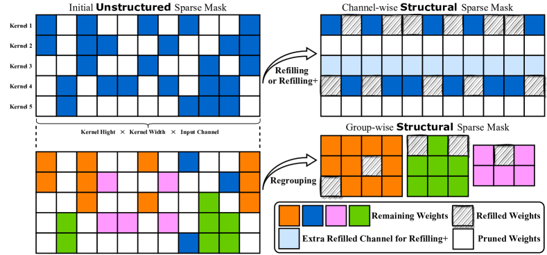
Figure 2: Overview of our proposals including refilling, refilling+, and regrouping, which turn unstructured sparse mask into channel-wise and group-wise structured sparse masks.

Pruning.

Network pruning is a technique that aims at eliminating the unnecessary model parameters (Blalock et al., 2020), which can effectively shrink models for the deployment on resource-constrained devices (LeCun et al., 1990; Hanson & Pratt, 1988). Pruning algorithms are roughly categorized into two groups: (1) unstructured pruning (LeCun et al., 1990; Han et al., 2015a, b; Ren et al., 2018; Zhang et al., 2018) with irregular sparse patterns; (2) structural pruning (He et al., 2017; Liu et al., 2017; Li et al., 2016; Hu et al., 2016; Wen et al., 2016; Hong et al., 2018) with structural sparse patterns such as layer-wise, channel-wise, block-wise, column-wise, etc..

Within the group of unstructured pruning methods, Han et al. (2015a, b) remove insignificant connections of models in the post-training stage, with respect to certain heuristics like weight/gradient magnitudes; during training sparsification is also another popular trend for pruning by leveraging $\ell_{0}$ regularization (Louizos et al., 2017) or alternating direction method of multipliers (ADMM) (Ren et al., 2018; Zhang et al., 2018). Recently, several pruning-at-initialization methods (Wang et al., 2020; Lee et al., 2019b; Tanaka et al., 2020) are proposed to identify critical unstructured connections for gradient-flow preserving, without any training. Although the unstructured sparse model has superior performance, it usually suffers from poor data locality and low parallelism (He et al., 2017; Mao et al., 2017; Wen et al., 2016), which make it hard to be accelerated in real-world hardware platforms.

On the contrary, structural pruning is more hardware-friendly at the cost of notable accuracy loss when the compression ratio increases. He et al. (2017); Liu et al. (2017) slim the network channels via $\ell_{1}$ regularization, and Bartoldson et al. (2019) selects important channels according to heuristics of feature maps. To combine the benefits of structural and unstructured pruning, hybrid pruning strategies have been introduced to pursue more general structural spares patterns which are also capable of acceleration. For example, convolution kernels with half regular sparsity (Chen et al., 2018) or pattern-based structural sparsity (Ma et al., 2020) or vector-wise (Zhu et al., 2019) and group-wise (Rumi et al., 2020) regular sparsity.

The lottery tickets hypothesis (LTH).

The lottery ticket hypothesis (LTH) (Frankle & Carbin, 2019) conjectures that there exists a sparse subnetwork called winning ticket within a dense network, whose performance can match with the dense network when training from the same initialization. With the assistance of weight rewinding techniques (Renda et al., 2020; Frankle et al., 2020a), the original LTH can be scaled up to larger networks and datasets. The existence of winning tickets are broadly verified under diverse contexts, such as image classification (Frankle & Carbin, 2019; Zhang et al., 2021; Chen et al., 2020a; Ma et al., 2021a; Gan et al., 2021; Chen et al., 2021c), natural language processing (Gale et al., 2019; Chen et al., 2020b), generative adversarial networks (Chen et al., 2021d, a), graph neural networks (Chen et al., 2021b), and reinforcement learning (Yu et al., 2020). However, all of the above LTH literature only locate unstructured sparse winning tickets, which can hardly bring hardware efficiency boost to real-world applications.

As the most related work, You et al. (2020) finds structural winning tickets at only low sparsity levels around $30\%$ in a few cases. It again reveals the complication and difficulty of identifying computation-friendly sparse patterns. Another concurrent work (Alabdulmohsin et al., 2021) investigates a generalized LTH with weight space factorization, which is orthogonal to our work.

Table 1: Implementation details which follow the standard settings in Ma et al. (2021b).

Settings CIFAR-10 CIFAR-100 Tiny-ImageNet ImageNet WRN-32-2 RN-18 MBNet-v1 VGG-16 WRN-32-2 RN-18 MBNet-v1 VGG-16 RN-50 RN-50 Batch Size 128 128 128 128 - - 64 - 32 - Weight Decay $1\times 10^{-4}$ $1\times 10^{-4}$ $1\times 10^{-4}$ $2\times 10^{-4}$ $2\times 10^{-4}$ $2\times 10^{-4}$ $2\times 10^{-4}$ $5\times 10^{-4}$ $5\times 10^{-4}$ $1\times 10^{-4}$ Learning Rate 0.1;$\times 0.1$ at 80,120 epoch of total 160 epochs 0.1;$\times 0.1$ at 30,60 epoch of total 95 epochs Optimizer SGD (Ruder, 2016) with a momentum of 0.9 Model Size $1.86$ M $11.22$ M $3.21$ M $14.72$ M $1.86$ M $11.22$ M $3.21$ M $14.72$ M $25.56$ M $25.56$ M

Sparse convolutional neural network acceleration on GPU.

Previous works have explored the acceleration of sparse convolution operations in two different directions. One direction is to design efficient implementation of unstructured pruned networks for improved data locality and utilization of hardware (Chen, 2018; Park et al., 2016). For example, Dong et al. (2019) proposes “Acorns” to accelerate the sparse computations of convolution kernels with an input sparsity. Peng et al. (2017) has proposed a matrix splitting algorithm for efficient inference of convolutional neural networks (CNN). Nvidia’s cuSPARSE library contains various efficient sparse matrix computation algorithms like SpMM on GPUs, drawing great attention to efficient scientific computing. Furthermore, advanced approaches are developed based on SpMM, such as Adaptive Sparse Tiling (ASpT) (Hong et al., 2019). ASpT significantly improves the data usage of SpMM and achieves the current state-of-the-art performance among SpMM implementation variants. Another direction focuses on more hardware-friendly pruning methods (Chen et al., 2018; Ma et al., 2020; Niu et al., 2020). During the model pruning, these works aim to maintain certain regular sparse patterns, which benefit the hardware processing/computing of corresponding sparse matrices. However, Chen et al. (2018) achieves unsatisfactory compression ratio, while the pruning methods used in Ma et al. (2020) and Niu et al. (2020) require dedicated compiler optimization to accelerate network execution.

3 Methodology

3.1 Notations and Preliminaries

Sparse subnetworks and pruning methods.

In this paper, we mainly follow the routine notations in (Frankle & Carbin, 2019; Renda et al., 2020). For a network $f(x;\theta)$ with input samples $x$ and model parameters $\theta$, a sparse subnetwork is a network $f(x;m\odot\theta)$ with a binary pruning mask $m\in\{0,1\}^{|\theta|}$, where $\odot$ is the element-wise product. In other words, it is a copy of dense network $f(x;\theta)$ with some weights fixed to $0$. If the non-fixed remaining weights are distributed irregularly, we call it unstructured sparse patterns (e.g., the left of Figure 2); if they are clustered into channels or groups, we name it structural sparse patterns (e.g., the right of Figure 2).

To obtain the desired sparse subnetworks, we consider and benchmark multiple classical pruning algorithms: (1) random pruning (RP) which usually works as a necessary baseline for the sanctity check (Frankle & Carbin, 2019); (2) one-shot magnitude pruning (OMP) by eliminating a part of model parameters with the globally smallest magnitudes (Han et al., 2015a); (3) the lottery ticket hypothesis (Frankle & Carbin, 2019) with iterative weight magnitude pruning (LTH-IMP or IMP for simplicity) (Han et al., 2015a). As adopted in LTH literature (Frankle & Carbin, 2019), we identify the sparse lottery tickets by iteratively removing the $20\%$ of remaining weight with the globally smallest magnitudes, and rewinding model weights to the original random initialization (Frankle & Carbin, 2019) or early training epochs (Frankle et al., 2020b; Chen et al., 2020a). In this paper, the model weights are rewound to the eighth epoch (i.e., the $5\%$ of the entire training process) for all CIFAR, Tiny-ImageNet, and ImageNet experiments. (4) pruning at initialization mechanisms. We choose several representative approaches such as SNIP (Lee et al., 2019a), GraSP (Wang et al., 2020), and SynFlow (Tanaka et al., 2020), which explore sparse patterns at random initialization with some gradient flow-based criterion. (5) Alternating Direction Method of Multipliers (ADMM) for punning. It is a well-known optimization-based pruning method (Niu et al., 2020; Zhang et al., 2018), which can obtain superior compression ratios with little performance degradation for deep neural networks. Note that all pruning approaches are mainly conducted over networks without counting their classification heads (Frankle & Carbin, 2019).

Structural winning tickets.

We begin by extending the original lottery tickets hypothesis to the context of structural sparse patterns. A subnetwork $f(x;m\odot\theta)$ is a structural winning ticket for an algorithm $\mathcal{A}^{\mathcal{T}}_{t}$ if it satisfies: ① training subnetworks $f(x;m\odot\theta)$ with algorithm $\mathcal{A}_{t}^{\mathcal{T}}$ results in performance measurement on task $\mathcal{T}$ no lower than training dense networks $f(x;\theta)$ with algorithm $\mathcal{A}^{\mathcal{T}}_{t}$, where $\theta$ is the original random initialization $\theta_{0}$ or early rewound weights like $\theta_{5\%}$, and $t$ is the training iterations; ② the non-zero elements in pruning mask $m$ are clustered as channels, groups or other hardware-friendly structural patterns.

Implementation details.

We conduct experiments on diverse combinations of network architectures and datasets. Specifically, we adopt Wide-ResNet-32-2 (Zagoruyko & Komodakis, 2016) (or WRN-32-2), ResNet-18 (He et al., 2016) (or RN-18), MobileNet-v1 (or MBNet-v1) (Howard et al., 2017), and VGG-16 (Simonyan & Zisserman, 2014) on both CIFAR-10 (Krizhevsky et al., 2009) and CIFAR-100 datasets. ResNet-50 (or RN-50) is evaluated on both Tiny-ImageNet (Le & Yang, 2015) and ImageNet (Deng et al., 2009) datasets. Table 1 includes more training and evaluation details of our experiments.

3.2 Refilling for Structural Patterns

It is well-known that the irregular sparsity patterns from unstructured magnitude pruning block the acceleration on practical hardware devices. To overcome the limitation, we propose a simple refilling strategy to reorganize the unstructured sparse patterns and make them more hardware friendly. Specifically, we first select important channels from the unstructured subnetwork according to certain criteria. The number of picked channels are depended on the desired sparsity level. Then, the pruned elements are grown back to be trainable (i.e., unpruned) and are reset to the same random initialization or early rewound weights. Lastly, the rest parameters in the remaining insignificant channels will be removed. In this way, we refill important channels and empty the rest to create a channel-wise structural sparse pattern that essentially brings computational reductions. Note that the picking criterion can be the number of remaining weights in the channel, or the channel’s weight statistics or feature statistics or salience scores, which are comprehensively investigated in the ablation (Section A2). The complete pipeline and illustration are summarized in Algorithm 2 and Figure 2, respectively.

Algorithm 1 IMP with rewinding step $i$

0:  $f(x;\theta_{0})$, unstructured sparsity $s$

0:  $f(x;m\odot\theta_{i})$

1:  Set the pruning mask $m=\bm{1}\in\mathbb{R}^{|\theta|}$

2:  Train $f(x;\theta_{0})$ for $i$ steps: $f(x;\theta_{i})=\mathcal{A}_{i}^{\mathcal{T}}(f(x;\theta_{0}))$

3:  while not reach sparsity $s$ do

4:     Train $f(x;m\odot\theta_{i})$ for $t-i$ steps: $f(x;m\odot\theta_{t})=\mathcal{A}_{t-i}^{\mathcal{T}}(f(x;m\odot\theta_{i}))$

5:     Pruning $20\%$ of remaining weight of $m\odot\theta_{t}$, and update $m$

6:  end while

Algorithm 2 IMP-Refill(+)

0:  $f(x;m\odot\theta_{i})$ with unstructured sparsity $s$ (Algo. 1)

0:  $f(x;m\odot\theta_{i})$ with channel-wise structural mask $m$ at sparsity $\tilde{s}$

1:  Calculate importance scores of each channel according to certain criterion

2:  Pick top-$k$ channels in $m$, refill back their $0$ (pruned) elements with $1$ (trainable) and update $m$, maintaining $\tilde{s}\sim s$

3:  Pick and refill back extra channels in $m$ with $\tilde{s}^{+}<s$ # Optional for Refill+

Algorithm 3 IMP-Regroup

0:  $f(x;m\odot\theta_{i})$ with unstructured sparsity $s$ from Algorithm 1, hyperparameters $t_{1}$, $t_{2}$, $b_{1}$, and $b_{2}$

0:  $f(x;m\odot\theta_{i})$ with group-wise structural mask $m$ at sparsity $s^{*}$

1:  while dense block can be found do

2:     Divide the rows of the sparse pruning mask $m$ into $t_{1}$ groups using hypergraph partitioning (hMETIS)

3:     for group $c_{i}\in\{c_{1},c_{2},\dots,c_{t_{1}}\}$  do

4:        if $c_{i}$ has $\geq b_{1}$ rows then

5:           Select columns in $c_{i}$ that has no less than $t_{2}$ non-zero items

6:           if $\geq b_{2}$ columns are selected then

7:              Group and Refill the selected columns as well as rows to a dense block, and update $m$

8:           end if

9:        end if

10:     end for

11:  end while

12:  Set other elements out of dense blocks to $0$

Here we provide a detailed description of how many and which channels we choose to refill. Our main experiments adopt the $\ell_{1}$ norm of channel weights as the picking criterion to score the channel importance due to its superior performance. Let $\theta^{l}\in\mathbb{R}^{c_{\mathrm{out}}\times n}$ denotes the parameters of the convolutional layer $l$, where $c_{\mathrm{out}}$ is the number of output channel and $n$ is the continued product of the number of input channel, channel height and weight, as shown in Figure 2. $\theta^{l}_{i}\in\mathbb{R}^{n}$ represents the weights in the $i$th kernel and $m^{l}_{i}\in\{0,1\}^{|\theta^{l}_{i}|}$ is the corresponding mask. We first calculate the $\ell_{1}$ norm of $m^{l}_{i}\odot\theta^{l}_{i}$, which is a summation of the absolute value of remaining weights in the kernel $i$. Then we use it to pick the top-$k$ scored kernels, which will be fully refilled. $k=\lceil s^{l}\times c_{\mathrm{out}}\times n\rceil$, where $s^{l}$ is the original layerwise sparsity and $c_{\mathrm{out}}\times n$ is the total number of weights in kernel $i$. Meanwhile, the rest $c_{\mathrm{out}}-k$ kernels are dropped for efficiency gains.

Furthermore, we propose a soft version, refilling+, to make a redemption for the aggressive nature of wiping out all remaining channels. It picks and re-actives an extra proportion of channels to slow down the network capacity reduction, as indicated by shallow blue blocks in Figure 2.

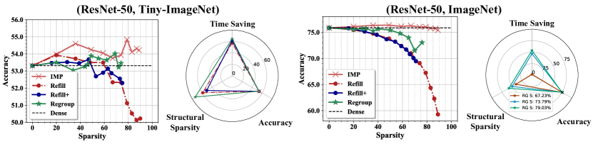
Figure 3: (Curve plots) Testing accuracy (%) over network sparsity (%) on Tiny-ImageNet and ImageNet datasets with ResNet-50 ($25.56$ M). (Radar plots) The end-to-end inference time saving of extreme structural winning tickets. Unstructured subnetworks or dense models do not have structural sparsity, and thus they are plotted as dots in the axes of accuracy in the corresponding radar plot. The rightmost plot includes three extreme regroup tickets with accuracy drop $<1\%$, where “RG S: $x\%$” indicates unstructured sparsity before regrouping.

3.3 Regrouping for Structural Patterns

Although proposed refilling+ reorganizes the unstructured mask and produces useful channel-wise structural subnetworks, it is rigid and inelastic since the smallest manageable unit is a kernel. In other words, the dense matrices in identified structural patterns have a restricted shape where one dimension must align with the kernel size $n$, i.e., the continued product of the number of input channels, channel height, and weight. Motivated by Rumi et al. (2020), we introduce a regrouping strategy (Figure 2) to create more fine-grained group-wise structural patterns with flexible shapes for remaining dense matrices.

$\rhd$ How to perform regrouping? Regrouping aims to find and extract dense blocks of non-pruned elements in the sparse weight matrix. These blocks have diverse shapes, as demonstrated in Figure 2, which are usually smaller in size compared to the original sparse matrix. Note that a channel/kernel can be regarded as a special case of the dense block.

As described in Algorithm 3, to achieve the goal, we first need to find similar rows and columns, and then bring them together. Specifically, We adopt the Jaccard similarity (Rumi et al., 2020; Jiang et al., 2020) among non-zero columns as the similarity between two rows in the sparse matrix, which is calculated as a cardinality ratio of the intersections to the union of non-zero columns. For instance, kernel $1$ and kernel $2$ in Figure 2 (upper left) share three columns in eight non-zero distinct columns, and their similarity is $\frac{3}{8}$. Then, if two rows have a larger similarity, they can form a denser block when we group them together. Take Figure 2 as an example. We can group kernel $1,2,3$’s non-zero columns $1,3,6,11$ with at least two elements together, which leads to the first orange dense block.

More precisely, we take the hypergraph partitioning in the regrouping algorithm to generate dense blocks. It treats each row and column from the sparse matrix as a node and hyperedge in the hypergraph, where hyperedge (i.e., column) connects the corresponding nodes (i.e., row). Then, the pair-wise similarity is leveraged to locate an optimal partitioning, which can be achieved with hMETIS. More details are referred to Rumi et al. (2020). After obtaining the desired dense blocks, we enable all their parameters to be trainable by refilling the corresponding pruned elements. Note that refilling these pruned weights does not cause any efficiency loss since the size of the blocks is fixed, while it potentially maximizes the usage of these blocks and brings accuracy gains. Meanwhile, the rest parameters not included in the dense blocks will be discarded, i.e., setting the corresponding position in binary mask $m$ to zero, for reducing the computational overhead as illustrated in Figure 2. It is because any parameters outside the dense blocks require extra weights loading and have little data reuse (Rumi et al., 2020), which harms the trade-off of accuracy and efficiency.

$\rhd$ How refilled / regrouped dense blocks be beneficial? We notice that the common tools like cuDNN (Chetlur et al., 2014) have a significant drawback that the inference time does not linearly change with the number of kernels, since they are only optimized for kernel matrices with a multiple of $32$ rows (Radu et al., 2019). For example, as stated in Rumi et al. (2020), a convolutional layer with $10$ kernels might have a similar inference time with a convolutional layer with $32$ kernels. However, the number of kernels in these dense blocks is almost arbitrary, so a more sophisticated GEMM-based efficient implementation (Rumi et al., 2020) is needed to accelerate better our refilled / regrouped structural patterns. Following Rumi et al. (2020), we split a kernel with $r$ rows into two parts: one has $[r/32]\times 32$ rows and the other one has $r$ mod $32$ rows. First, we directly apply the standard GEMM-based convolution algorithm with shared memory to cache the input and output matrix. For the second part, due to the poor data reuse of input matrices, we choose to cache the kernel and output matrices for an improved cache hit rate and overall performance. More details are referred to Rumi et al. (2020).

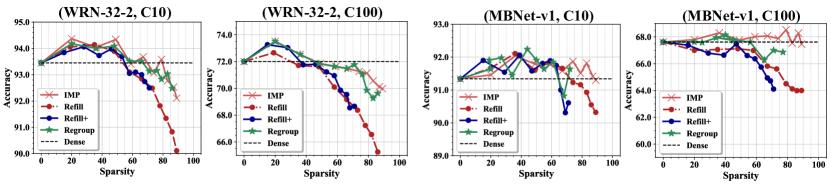
Figure 4: Testing accuracy (%) over sparsity (%) on CIFAR-10/100 with Wide-ResNet-32-2 ($1.86$ M) and MobileNet-v1 ($3.21$ M).

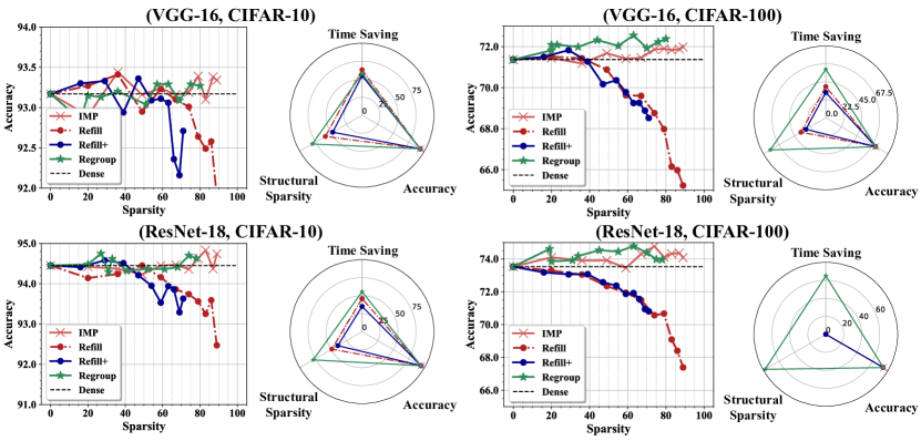
Figure 5: (Curve plots) Testing accuracy (%) over sparsity (%) on CIFAR-10/100 with large models VGG-16 ($14.72$ M) and RN-18 ($11.22$ M). (Radar plots) The end-to-end inference time saving of extreme structural winning tickets. Note that unstructured subnetworks or dense models do not have structural sparsity, and thus they are plotted as dots in the axes of accuracy in the corresponding radar plot.

4 The Existence of Structural Winning Ticket

Tiny-ImageNet and ImageNet.

In this section, we reveal the existence of our proposed structural winning tickets on ImageNet and Tiny-ImageNet with ResNet-50 backbone. Results of unstructured IMP, channel-wise structural IMP-Refill(+), and group-wise structural IMP-Regroup are collected in the Figure 3. The end-to-end inference time of obtained structural winning tickets with extreme sparsity levels are presented, which is calculated on a single 2080 TI GPU with a batch size of $64$. Extreme sparsity is defined as maximum sparsity when the subnetwork has superior accuracy to its dense counterpart.

From Tiny-ImageNet results in Figure 3 (left), several positive observations can be drawn: ❶ Structural winning tickets with $60\%$ channel-wise structural sparsity and $74\%$ group-wise structural sparsity are located by IMP-Refill and IMP-Regroup respectively, which validate the effectiveness of our proposals. ❷ Although at the high sparsity levels (i.e., $>50\%$), IMP-Refill+ outperforms IMP-Refill if they are from the same unstructured IMP subnetworks. Considering the overall trade-off between channel-wise structural sparsity and accuracy, IMP-Refill appears a clear advantage. A possible explanation is that refilling+ seems to bring undesired channels which potentially result in a degraded performance trade-off. ❸ IMP-Regroup performs better at high sparsities. It is within expectation since fine-grained group-wise structural patterns tend to make the networks be more amenable to pruning. ❹ Extreme channel- / group-wise structural winning tickets with $45\%\sim 50\%$ / $74\%$ sparsity from IMP-Refill(+) / IMP-Regroup achieve $57.53\%\sim 61.79\%$ / $64.84\%$ GPU running time savings, without sacrificing accuracies.

As for large-scale ImageNet experiments, the conclusion are slightly different: ❶ There is almost no difference between the performance of IMP-Refill and IMP-Refill+, and both can not find channel-wise structural winning tickets. But it seems to suggest our picking rule (i.e., channel weights’ $\ell_{1}$ norm) provides a great estimation for channel importance, although it is too aggressive for ImageNet experiments. ❷ The group-wise structural winning ticket at $31\%$ sparsity still exist in (RN-50, ImageNet), while the low sparsity brings limited $1\%$ time savings. For a better efficiency and performance trade-off, IMP-Regroup is capable of locating structural subnetworks at $51\%$ / $58\%$ sparsity with $53.75\%$ / $60.23\%$ time savings and $0.33\%$ / $0.95\%$ accuracy drop.

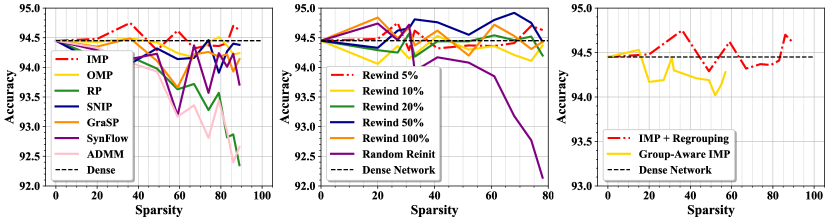
Figure 6: (Left) Performance of structural tickets grouped from diverse initial unstructured masks. (Middle) Performance of group-wise structural tickets with different weight rewinding. (Right) Performance comparisons between IMP-Regroup and group-aware IMP as described in Algorithm 4. Testing accuracies (%) over network sparsity levels (%) are reported on (RN-18,C10).

CIFAR with diverse network architectures.

We then validate our approaches on CIFAR-10/100 (C10/100) with diverse network backbones including Wide-ResNet-32-2, MobileNet-v1, VGG-16, and ResNet-18. Based on the extensive results in Figure 4 and 5, we find: ❶ On {(WRN-32-2,C10), (WRN-32-2,C100), (MBNet-v1,C10), (MBNet-v1,C100), (VGG-16,C10), (VGG-16,C100), (RN-18,C10), (RN-18,C100)} schemes, we consistently disclose the existence of structural winning tickets with {$53\%$, $28\%$, $67\%$, $0\%$, $60\%$, $40\%$, $50\%$, $0\%$} channel-wise sparsity and {$66\%$, $36\%$, $72\%$, $56\%$, $80\%$, $80\%$, $78\%$, $78\%$} group-wise sparsity from IMP-Refill(+) and IMP-Regroup, respectively. ❷ With the same network, pursuing channel-wise sparse patterns on CIFAR-100 is more challenging than it on CIFAR-10, possibly due to the larger dataset complexity. On the same dataset, larger networks tend to have larger extreme sparsities for both channel- and group-wise structural winning tickets, with the exception of IMP-Refill(+) on (RN-18, C100). ❸ At the middle sparsity levels (i.e., $<50\%$), IMP-Regroup behaves closely to IMP-Refill(+), while IMP-Regroup has a superior performance at high sparsity levels. ❹ Up to {$57.75\%$, $60.60\%$, $55.45\%$, $64.93\%$} GPU running time savings are obtained by group-wise structural winning tickets with undamaged performance on {(VGG-16,C10), (VGG-16,C100), (RN-18,C10), (RN-18,C100)}, which surpass IMP, IMP-Refill(+), and dense models by a significant efficiency margin. A exception is that IMP-Refill on (VGG-16,C10) achieves the best time savings, i.e., $63.11\%$.

Layer-wise speedups.

Figure 7 and A10 shows the layer-wise speedup performance of convolution operations in VGG-16’s extreme structured winning tickets from different algorithms.IMP-Regroup presents impressive layer-wise speedups up to $6.67$x compared to others, especially on the last a few layers (e.g., conv. $12$). The possible reasons lie in two aspects: ($i$) the latter layers reach a larger compression ratio and have greater potentials for acceleration; ($ii$) the regrouping algorithm prefers convolutional layers (i.e., latter layers in VGG-16) with a larger number of kernels which benefits to group appropriate dense blocks, as also suggested by Rumi et al. (2020).

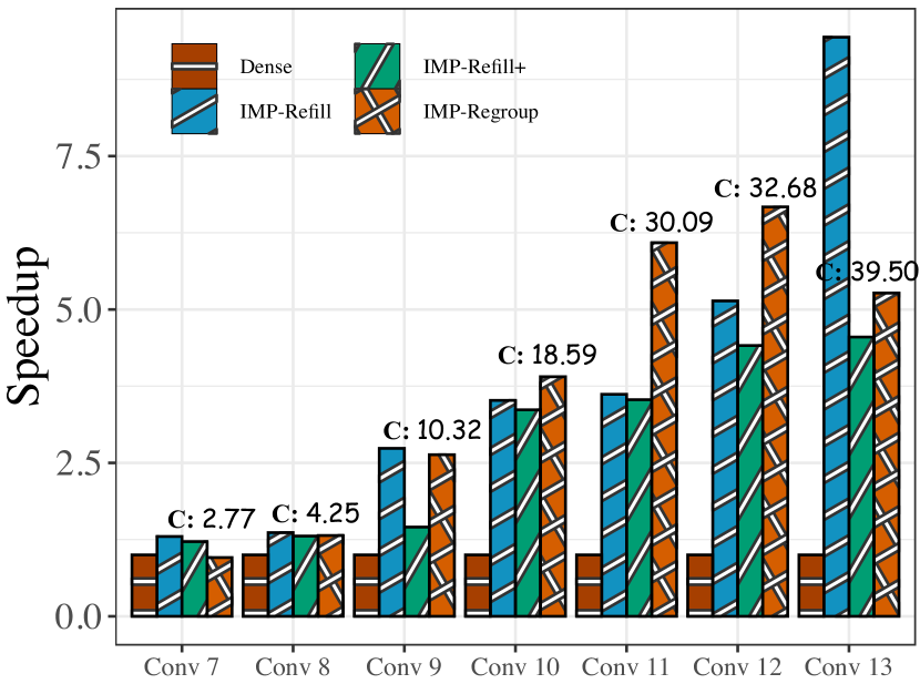
Figure 7: The layer-wise performance of convolution operations in extreme structural winning tickets of (VGG-16, C10). The first six conv. operations are omitted since there is no meaningful speedup, coincided with Rumi et al. (2020). Marks like “C: 2.77” indicate the layer-wise compression ratio of IMP-Regroup.

5 Ablation Study and Visualization

Different sources of unstructured masks.

Intuitively, the initial unstructured sparse mask should plays an essential role in the achievable performance of our proposed “post-processing techniques”. We therefore conduct a comprehensive ablation study about the various sources of the initial sparse masks in Figure 6, including IMP, OMP, RP, SNIP, GraSP, SynFlow, and ADMM. The details of comparison methods are in Section 3.1. We observe that IMP and OMP provide initial unstructured masks with the top-$2$ highest quality for our regrouping algorithm, in terms of the train-from-scratch accuracy of grouped structural subnetworks.

Different initialization for the re-training.

Initialization (Frankle & Carbin, 2019; Renda et al., 2020) as another key factor in LTH, also contributes significantly to the existence of winning tickets. To exhaustively investigate the effect from different initialization (e.g., rewound weights), we launch experiments started from diverse rewound weights ($\{5\%,10\%,20\%,50\%,100\%\}$ of total training epochs) as well as a random re-initialization. In Figure 6, using $50\%$ rewound weight reaches the overall best performance; other weight rewinding setups perform similarly and clearly surpass random re-initializing at sparsity levels $>30\%$.

Group-aware IMP.

This work mainly focuses on the post-processing of unstructured sparse masks. Another possibility is integrating regrouping into IMP by alternatively performing unstructured magnitude pruning and regrouping, which we term as group-aware IMP. From Fig. 6, it has a worse performance due to the stricter constraint on sparse patterns, compared to IMP-Regroup.

Extra study.

More investigations about ($1$) transfer tickets and training efficiency; ($2$) comparison with random tickets; ($3$) ablation on different training settings; ($4$) FLOPs saving; ($5$) visualization of sparse masks are in Appendix A2.

6 Conclusion

In this paper, we challenge the “common sense” that an identified IMP winning ticket can only have unstructured sparsity, which severely limits its practical usage due to the irregular patterns. We for the first time demonstrate the existence of structural winning tickets by leveraging post-processing techniques, i.e., refilling(+) and regrouping. The located channel- and group-wise structural subnetworks achieve significant inference speedups up to $6.67$x on hardware platforms. In this sense, our positive results bridge the gap between the lottery ticket hypothesis and practical accelerations in real-world scenarios. We would be interested in examining LTH with more effective structural sparsity for real-time mobile computing in future work.

Appendix A1 More Implementation Details

Group-aware IMP.

Here we provides the detailed procedures of group-aware IMP in Algorithm 4. Intuitively, it embeds regrouping (Algorithm 3) into IMP (Algorithm 1) by performing regrouping on the unstructured mask $m$ from each IMP round.

Algorithm 4 Group-aware IMP

0:  $f(x;\theta_{0})$, group-wise structural sparsity $s$

0:  $f(x;m\odot\theta_{i})$ with group-wise structural sparse mask $s$

1:  Set the pruning mask $m=\bm{1}\in\mathbb{R}^{|\theta|}$Train $f(x;\theta_{0})$ to rewinding step $i$: $f(x;\theta_{i})=\mathcal{A}_{i}^{\mathcal{T}}(f(x;\theta_{0}))$

2:  while not reach sparsity $s$ do

3:     Train $f(x;m\odot\theta_{i})$ to step $t$: $f(x;m\odot\theta_{t})=\mathcal{A}_{t-i}^{\mathcal{T}}(f(x;m\odot\theta_{i}))$

4:     Pruning $20\%$ of remaining weight of $m\odot\theta_{t}$, and update $m$

5:     Refining the unstructured mask $m$ by performing regrouping, as shown in Algorithm 3

6:  end while

Profiling.

To compute the GPU running time of regrouped convolution layers, we adopt their CUDA C/C++ implementation. Our results do not include the running time of normalization and activation layers, following the standard in Rumi et al. (2020). For a fair calculation, we feed the same input features to convolution layers that belong to the same model. For ResNet-18 and VGG-16, the size of the input features is $(64,64,127,127)$. For ResNet-50, the size of input features is $(64,64,64,64)$. The GPU we use for profiling is NVIDIA RTX 2080 TI, with a CUDA version of $10.2$ and a cuDNN (Chetlur et al., 2014) version of $7.6.5$.

Appendix A2 More Experiment Results

Different channel picking criterion for refilling.

We ablation the channel picking criterion for IMP-Refill(+), including ❶ the $\ell_{1}$ norm of channel’s remaining weight, ❷ the $\ell_{1}$ or $\ell_{2}$ norms of channel’s feature map, ❸ the number of remaining weights in the channel, ❹ the channel’s saliency score (Molchanov et al., 2019). Experiment results are collected in Figure A8, which demonstrate the superior performance of IMP-Refill w. $\ell_{1}$ of channel weights (yellow curve in Figure A8).

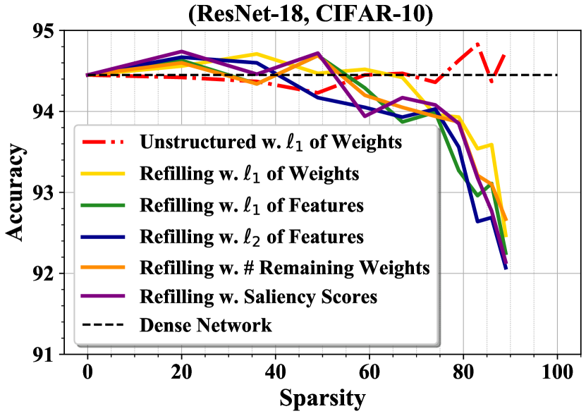
Figure A8: Performance of structural tickets refilled by diverse channel picking criterion. Testing accuracies (%) over network sparsity levels (%) are reported on (RN-18,C10).

Transfer tickets and training efficiency.

We investigate the transferability of our found (fine-grained) structural winning tickets, which grants the extra bonus of training efficiency to our proposals. Specifically, following the setups in Chen et al. (2020a), we first identify refilled and regrouped structural winning tickets in ResNet-18 on ImageNet, and then transfer them to the downstream CIFAR-10 task. Transfer results are presented in Table A2. Compared to the dense network baseline ($95.37\%$), IMP-Refill locates channel-wise structural (transfer) winning tickets at the sparsity around $36\%$, and IMP-Regroup locates group-wise structural (transfer) winning tickets at a higher sparsity (more than $56.00\%$). Such an encouraging transfer study means that we can even replace the full model with a much smaller subnetwork while maintaining an undamaged downstream performance. And this is also why our IMP-Regroup and IMP-Refill obtain $7.14\%\sim 34.67\%$ and $34.53\%$ training time savings during downstream training with matched or even improved generalization. Note that this efficient training is an extra benefits of our proposal, in addition to impressive inference efficiency.

Table A2: Transfer accuracy ($\%$), time saving ($\%$) and remaining weights ($\%$) on ResNet-50 with CIFAR-10. IMP-Refill and IMP-Regroup are evaluated. The baseline accuracy of dense network is $95.37\%$.

IMP-Refill
Remaining Weight	Transfer Accuracy	Time Savings
64.14%	95.81%	34.53%
51.37%	95.14%	48.10%
41.01%	94.51%	60.67%
32.76%	94.38%	65.98%
26.17%	94.19%	69.04%
20.97%	94.11%	71.08%
IMP-Regroup
Remaining Weight	Transfer Accuracy	Time Savings
59.43%	95.65%	7.14%
51.84%	95.39%	21.85%
43.99%	95.51%	34.67%

Comparison with random tickets.

As a sanity check, we conduct a comparison with random tickets (Frankle & Carbin, 2019) which are trained from random re-initialization. Experiments results on (RN-18, C10) are collected in Table A3 and A4. We show that random tickets have obviously inferior performance, which suggests that our identified refilled and regrouped subnetworks are highly non-trivial (fine-grained) structural winning tickets.

Table A3: Testing accuracy ($\%$) of IMP-Refill with rewinding weights (Ours) and random re-initialization (Random Tickets).

IMP Round	Remaining Weight	Accuracy (Ours)	Accuracy (Random Tickets)
1	80.29$\%$	94.14%	94.04%
2	64.49$\%$	94.24%	93.96%
3	51.43$\%$	94.45%	94.20%
4	41.24$\%$	94.16%	93.98%
5	32.97$\%$	93.86%	93.53%

Table A4: Testing accuracy ($\%$) of IMP-Regroup with rewinding weights (Ours) and random re-initialization (Random Tickets).

IMP Round	Remaining Weight	Accuracy (Ours)	Accuracy (Random Tickets)
1	80.00$\%$	94.48%	94.19%
2	72.95$\%$	94.75%	93.42%
3	69.37$\%$	94.29%	93.58%
4	67.12$\%$	94.62%	93.84%
5	58.54$\%$	94.32%	93.76%

Different training settings.

To validate our algorithm’s effectiveness under different training configurations, we perform extra experiments with VGG-16(+), WRN-32-2(+), and RN-50(+). The changes of training settings are summarized as below:

1. For VGG-16(+), we increase the number of training epochs to $240$, and decay the learning rate at $150$-th, $180$-th, and $210$-th epoch.

2. For WRN-32-2(+), we do not split the official training set into the a training and a validation set as our other experiments did. We also report the best validation accuracy instead of the best test accuracy. The number of training epochs is increased to $240$ and the learning rate is decayed at $150$-th, $180$-th, and $210$-th epoch.

3. For RN-50(+), we replace the first convolution layer to be of kernel size $3$, padding size $1$, and strides $1$.

$\rhd$ VGG-16(+) on C100. As shown in Table A5, we demonstrated that our conclusions are still hold: IMP-Regroup can locate structural winning tickets at very high sparsity levels (e.g., $>75\%$).

Table A5: Testing accuracy ($\%$) and remaining weights ($\%$) on CIFAR-100 with VGG-16(+). IMP, IMP-Refill, and IMP-Regroup are evaluated. The baseline accuracy of dense network is $73.43\%$.

Round	IMP		IMP-Refill		IMP-Regroup
	Remaining Weight	Accuracy	Remaining Weight	Accuracy	Remaining Weight	Accuracy
1	80.00%	73.64	80.17%	73.43	82.36%	73.63
2	64.00%	73.80	64.06%	72.87	80.00%	73.81
3	51.20%	73.67	51.31%	72.67	69.46%	74.31
4	40.96%	74.01	41.08%	71.37	62.61%	73.94
5	32.77%	74.27	32.85%	70.79	56.09%	75.05
6	26.21%	74.56	26.33%	71.07	46.53%	74.98
7	20.97%	74.58	21.03%	69.42	38.18%	75.24
8	16.78%	74.52	16.94%	68.75	30.98%	74.68
9	13.42%	74.42	13.42%	67.25	25.27%	75.25

$\rhd$ WRN-32-2(+) on C100. As shown in Table A6, we find consistent observations: IMP-Regroup locates structural winning tickets at about $75\%$ sparsity, and IMP-Refill identifies structural winning tickets at $20\%$ sparsity.

Table A6: Testing accuracy ($\%$) and remaining weights ($\%$) on CIFAR-100 with WideResNet-32-2(+). IMP, IMP-Refill, and IMP-Regroup are evaluated. The baseline accuracy of dense network is $75.53\%$.

Round	IMP		IMP-Refill		IMP-Regroup
	Remaining Weight	Accuracy	Remaining Weight	Accuracy	Remaining Weight	Accuracy
1	80.00%	76.21	80.00%	75.46	80.00%	75.98
2	64.00%	75.78	64.06%	74.59	64.00%	76.19
3	51.20%	76.02	51.51%	73.53	51.20%	76.13
4	40.96%	75.92	41.51%	72.95	40.96%	75.88
6	26.21%	75.74	26.53%	70.91	26.27%	75.78
7	20.97%	75.92	21.11%	69.55	21.76%	74.74
8	16.78%	75.87	17.11%	67.74	18.14%	73.85
9	13.42%	75.41	13.67%	65.73	14.85%	72.99

Table A7: Testing accuracy ($\%$) and remaining weights ($\%$) on Tiny-ImageNet with ResNet-50(+). IMP, IMP-Refill, and IMP-Regroup are evaluated. The baseline accuracy of dense network is $65.33\%$.

Round	IMP		IMP-Refill		IMP-Regroup
	Remaining Weight	Accuracy	Remaining Weight	Accuracy	Remaining Weight	Accuracy
1	80.00%	65.44	80.30%	65.27	80.15%	65.51
2	64.00%	65.69	64.16%	63.40	68.25%	65.16
3	51.20%	65.50	51.42%	61.89	58.19%	65.21
4	40.96%	65.73	41.08%	60.43	54.19%	64.42
5	32.77%	65.23	32.85%	59.64	51.75%	64.52

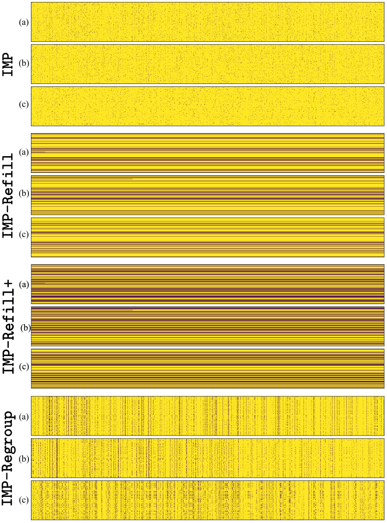
Figure A9: Sparse mask visualizations of the extreme winning tickets from IMP (unstructured), IMP-Refill(+) (channel-wise structural), and IMP-Regroup (group-wise structural) on (VGG-16,C10). The darker color indicates the remaining unpruned elements. (a,b,c) are the last three conv. layers.

$\rhd$ RN-50(+) on Tiny-ImageNet. Experimental results in Table A7 suggest that: IMP-Regroup locates structural winning tickets at about $42\%$ sparsity, and IMP-Refill discovers structural winning tickets at $20\%$ sparsity, which echo our findings in the main text.

FLOPs saving.

For a sufficient evaluation, we calculate the FLOPs of diverse subnetworks from VGG-16 on CIFAR-10 dataset. The FLOPs of a dense VGG-16 is about $0.314$G. We select sparsity levels across different methods as similar as possible for a better comparison. Subnetworks from IMP-Refill, IMP-Refill+, and IMP-Regroup at sparsity levels of {$32.84\%$, $46.41\%$, $20.12\%$} have {$0.089$G, $0.122$G, $0.093$G} FLOPs, respectively. It is noteworthy that Refill and Refill+ trim down the input and output channels of a convolution layer while Regroup cannot. Thus, Refill and Refill+ can save more FLOPs under a similar sparsity level.

Visualization of sparse masks.

Figure A9 visualizes different types of obtained sparse masks from (VGG-16,C10). Sub-figures (a,b,c) plot the mask matrices of size $c_{\mathrm{out}}\times n$ for certain layers. Similar to the illustration in Figure 2, IMP-Refill(+) masks show clear kernel-wise sparse patterns across the rows, and IMP-Regroup masks present fine-grained structural sparse patterns capable of forming neat dense blocks after regrouping.

More results of layer-wise speedups.

Figure A10 presents extra layer-wise speedup results of VGG-16 on CIFAR-100. Similar observations to Figure 7 can be obtain.

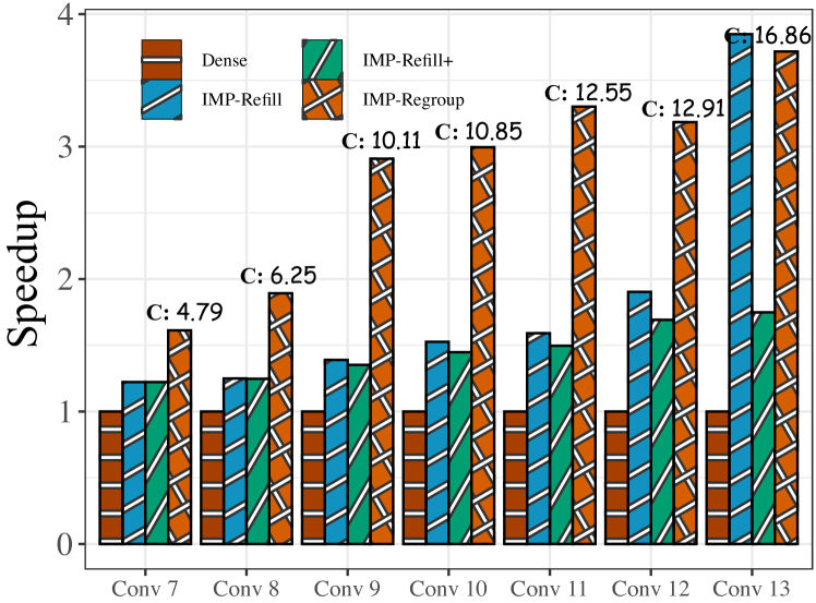
Figure A10: The layer-wise performance of convolution operations in extreme structural winning tickets of (VGG-16, C10). The first six conv. operations are omitted since there is no meaningful speedup, coincided with Rumi et al. (2020). Marks like “C: 2.77” indicate the layer-wise compression ratio of IMP-Regroup.

Different visualizations of the radar plots.

We offer an alternative histogram visualization (Figure A11) for radar plots in the main text. In each histogram, four approaches are reported: Dense, IMP-Refill, IMP-Refill+, and IMP-Regroup. Dense as the compared baseline with zero time saving, so the corresponding bars are always unseen from the charts.

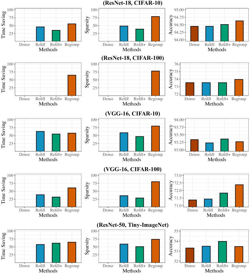
Figure A11: Time saving ($\%$), sparsity level ($\%$), and test accuracy ($\%$) of various models {ResNet-18, VGG-19, ResNet-50} on different datasets {CIFAR-10/100, Tiny ImageNet}.

Comparison to NAS and SOTA structure pruning methods.

We conduct extra experiments with a neural architecture search (NAS) based approach, i.e., ABC pruner (Lin et al., 2020). Specifically, it searches the channel numbers per layer, and then the derived structure will be trained from the same initialization. At the same sparsity level $77\%$, our IMP-Refill surpasses the ABC pruner by $1.5\%$ accuracy, which demonstrates the superiority of located refill tickets. More sparse levels are presented in Fig. A12 (C1).

Under the same setup of training from scratch, we further compare our proposal with SCOP (Tang et al., 2020) and observe that ours ($94.16\sim 94.62\%$) outperform SCOP ($93.48\%$) by up to $1.14\%$ accuracy at $\sim 41\%$ sparsity. More sparse levels are collected in Fig. A12 (C2).

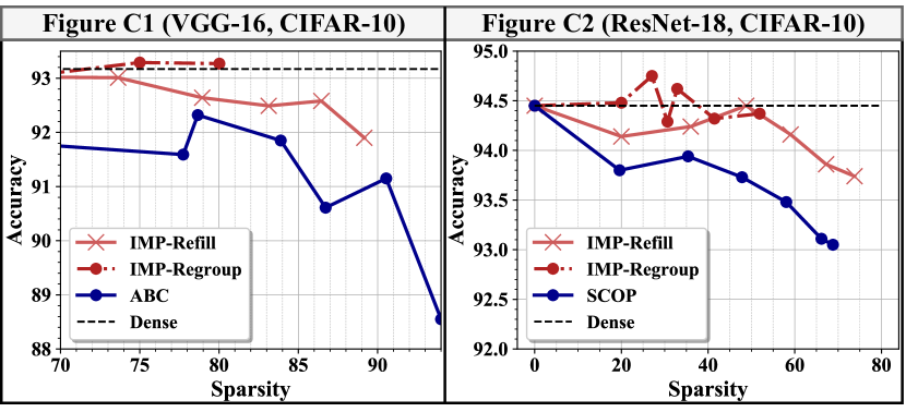
Figure A12: Comparisons with NAS and SOTA structural pruning.

References

- Alabdulmohsin et al. (2021) Alabdulmohsin, I., Markeeva, L., Keysers, D., and Tolstikhin, I. A generalized lottery ticket hypothesis. arXiv preprint arXiv:2107.06825, 2021.
- Bartlett et al. (2021) Bartlett, P. L., Montanari, A., and Rakhlin, A. Deep learning: a statistical viewpoint. arXiv preprint arXiv:2103.09177, 2021.
- Bartoldson et al. (2019) Bartoldson, B. R., Morcos, A. S., Barbu, A., and Erlebacher, G. The generalization-stability tradeoff in neural network pruning. arXiv preprint arXiv:1906.03728, 2019.
- Blalock et al. (2020) Blalock, D., Ortiz, J. J. G., Frankle, J., and Guttag, J. What is the state of neural network pruning? arXiv preprint arXiv:2003.03033, 2020.
- Brown et al. (2020) Brown, T. B., Mann, B., Ryder, N., Subbiah, M., Kaplan, J., Dhariwal, P., Neelakantan, A., Shyam, P., Sastry, G., Askell, A., et al. Language models are few-shot learners. arXiv preprint arXiv:2005.14165, 2020.
- Chen et al. (2018) Chen, C.-F., Oh, J., Fan, Q., and Pistoia, M. Sc-conv: Sparse-complementary convolution for efficient model utilization on cnns. In 2018 IEEE International Symposium on Multimedia (ISM), pp. 97–100. IEEE, 2018.
- Chen et al. (2020a) Chen, T., Frankle, J., Chang, S., Liu, S., Zhang, Y., Carbin, M., and Wang, Z. The lottery tickets hypothesis for supervised and self-supervised pre-training in computer vision models. arXiv preprint arXiv:2012.06908, 2020a.
- Chen et al. (2020b) Chen, T., Frankle, J., Chang, S., Liu, S., Zhang, Y., Wang, Z., and Carbin, M. The lottery ticket hypothesis for pre-trained bert networks. arXiv preprint arXiv:2007.12223, 2020b.
- Chen et al. (2021a) Chen, T., Cheng, Y., Gan, Z., Liu, J., and Wang, Z. Ultra-data-efficient gan training: Drawing a lottery ticket first, then training it toughly. arXiv preprint arXiv:2103.00397, 2021a.
- Chen et al. (2021b) Chen, T., Sui, Y., Chen, X., Zhang, A., and Wang, Z. A unified lottery ticket hypothesis for graph neural networks, 2021b.
- Chen (2018) Chen, X. Escort: Efficient sparse convolutional neural networks on gpus. arXiv preprint arXiv:1802.10280, 2018.
- Chen et al. (2021c) Chen, X., Chen, T., Zhang, Z., and Wang, Z. You are caught stealing my winning lottery ticket! making a lottery ticket claim its ownership. Advances in Neural Information Processing Systems, 34, 2021c.
- Chen et al. (2021d) Chen, X., Zhang, Z., Sui, Y., and Chen, T. {GAN}s can play lottery tickets too. In International Conference on Learning Representations, 2021d. URL https://openreview.net/forum?id=1AoMhc_9jER.
- Chetlur et al. (2014) Chetlur, S., Woolley, C., Vandermersch, P., Cohen, J., Tran, J., Catanzaro, B., and Shelhamer, E. cudnn: Efficient primitives for deep learning. arXiv preprint arXiv:1410.0759, 2014.
- Deng et al. (2009) Deng, J., Dong, W., Socher, R., Li, L.-J., Li, K., and Fei-Fei, L. Imagenet: A large-scale hierarchical image database. In 2009 IEEE conference on computer vision and pattern recognition, pp. 248–255. Ieee, 2009.
- Dong et al. (2019) Dong, X., Liu, L., Zhao, P., Li, G., Li, J., Wang, X., and Feng, X. Acorns: A framework for accelerating deep neural networks with input sparsity. In 2019 28th International Conference on Parallel Architectures and Compilation Techniques (PACT), pp. 178–191. IEEE, 2019.
- Du et al. (2018) Du, S. S., Zhai, X., Poczos, B., and Singh, A. Gradient descent provably optimizes over-parameterized neural networks. arXiv preprint arXiv:1810.02054, 2018.
- Frankle & Carbin (2019) Frankle, J. and Carbin, M. The lottery ticket hypothesis: Finding sparse, trainable neural networks. In International Conference on Learning Representations, 2019. URL https://openreview.net/forum?id=rJl-b3RcF7.
- Frankle et al. (2020a) Frankle, J., Dziugaite, G. K., Roy, D., and Carbin, M. Linear mode connectivity and the lottery ticket hypothesis. In International Conference on Machine Learning, pp. 3259–3269. PMLR, 2020a.
- Frankle et al. (2020b) Frankle, J., Schwab, D. J., and Morcos, A. S. The early phase of neural network training. In International Conference on Learning Representations, 2020b. URL https://openreview.net/forum?id=Hkl1iRNFwS.
- Gale et al. (2019) Gale, T., Elsen, E., and Hooker, S. The state of sparsity in deep neural networks. arXiv preprint arXiv:1902.09574, 2019.
- Gan et al. (2021) Gan, Z., Chen, Y.-C., Li, L., Chen, T., Cheng, Y., Wang, S., and Liu, J. Playing lottery tickets with vision and language. arXiv preprint arXiv:2104.11832, 2021.
- Han et al. (2015a) Han, S., Mao, H., and Dally, W. J. Deep compression: Compressing deep neural networks with pruning, trained quantization and huffman coding. arXiv preprint arXiv:1510.00149, 2015a.
- Han et al. (2015b) Han, S., Pool, J., Tran, J., and Dally, W. J. Learning both weights and connections for efficient neural networks. arXiv preprint arXiv:1506.02626, 2015b.
- Han et al. (2016) Han, S., Liu, X., Mao, H., Pu, J., Pedram, A., Horowitz, M. A., and Dally, W. J. Eie: efficient inference engine on compressed deep neural network. In ISCA, 2016.
- Hanson & Pratt (1988) Hanson, S. and Pratt, L. Comparing biases for minimal network construction with back-propagation. Advances in neural information processing systems, 1:177–185, 1988.
- He et al. (2016) He, K., Zhang, X., Ren, S., and Sun, J. Deep residual learning for image recognition. In Proceedings of the IEEE conference on computer vision and pattern recognition, pp. 770–778, 2016.
- He et al. (2017) He, Y., Zhang, X., and Sun, J. Channel pruning for accelerating very deep neural networks. In Proceedings of the IEEE International Conference on Computer Vision (ICCV), pp. 1389–1397, 2017.
- Hoefler et al. (2021) Hoefler, T., Alistarh, D., Ben-Nun, T., Dryden, N., and Peste, A. Sparsity in deep learning: Pruning and growth for efficient inference and training in neural networks. arXiv preprint arXiv:2102.00554, 2021.
- Hong et al. (2018) Hong, C., Sukumaran-Rajam, A., Bandyopadhyay, B., Kim, J., Kurt, S. E., Nisa, I., Sabhlok, S., Çatalyürek, U. V., Parthasarathy, S., and Sadayappan, P. Efficient sparse-matrix multi-vector product on gpus. Association for Computing Machinery, 2018.
- Hong et al. (2019) Hong, C., Sukumaran-Rajam, A., Nisa, I., Singh, K., and Sadayappan, P. Adaptive sparse tiling for sparse matrix multiplication. In Proceedings of the 24th Symposium on Principles and Practice of Parallel Programming, pp. 300–314, 2019.
- Howard et al. (2017) Howard, A. G., Zhu, M., Chen, B., Kalenichenko, D., Wang, W., Weyand, T., Andreetto, M., and Adam, H. Mobilenets: Efficient convolutional neural networks for mobile vision applications. arXiv preprint arXiv:1704.04861, 2017.
- Hu et al. (2016) Hu, H., Peng, R., Tai, Y.-W., and Tang, C.-K. Network trimming: A data-driven neuron pruning approach towards efficient deep architectures. arXiv preprint arXiv:1607.03250, 2016.
- Jiang et al. (2020) Jiang, P., Hong, C., and Agrawal, G. A novel data transformation and execution strategy for accelerating sparse matrix multiplication on gpus. PPoPP ’20. Association for Computing Machinery, 2020.
- Kaplan et al. (2020) Kaplan, J., McCandlish, S., Henighan, T., Brown, T. B., Chess, B., Child, R., Gray, S., Radford, A., Wu, J., and Amodei, D. Scaling laws for neural language models. arXiv preprint arXiv:2001.08361, 2020.
- Krizhevsky et al. (2009) Krizhevsky, A., Hinton, G., et al. Learning multiple layers of features from tiny images. 2009.
- Le & Yang (2015) Le, Y. and Yang, X. Tiny imagenet visual recognition challenge. CS 231N, 7:7, 2015.
- LeCun et al. (1990) LeCun, Y., Denker, J. S., and Solla, S. A. Optimal brain damage. In Advances in neural information processing systems, pp. 598–605, 1990.
- Lee et al. (2019a) Lee, N., Ajanthan, T., and Torr, P. Snip: Single-shot network pruning based on connection sensitivity. In International Conference on Learning Representations (ICLR), 2019a.
- Lee et al. (2019b) Lee, N., Ajanthan, T., and Torr, P. Snip: Single-shot network pruning based on connection sensitivity. In International Conference on Learning Representations, 2019b. URL https://openreview.net/forum?id=B1VZqjAcYX.
- Li et al. (2016) Li, H., Kadav, A., Durdanovic, I., Samet, H., and Graf, H. P. Pruning filters for efficient convnets. arXiv preprint arXiv:1608.08710, 2016.
- Lin et al. (2020) Lin, M., Ji, R., Zhang, Y., Zhang, B., Wu, Y., and Tian, Y. Channel pruning via automatic structure search. arXiv preprint arXiv:2001.08565, 2020.
- Liu et al. (2017) Liu, Z., Li, J., Shen, Z., Huang, G., Yan, S., and Zhang, C. Learning efficient convolutional networks through network slimming. In Proceedings of the IEEE International Conference on Computer Vision, pp. 2736–2744, 2017.
- Louizos et al. (2017) Louizos, C., Welling, M., and Kingma, D. P. Learning sparse neural networks through regularization. arXiv preprint arXiv:1712.01312, 2017.
- Ma et al. (2021a) Ma, H., Chen, T., Hu, T.-K., You, C., Xie, X., and Wang, Z. Good students play big lottery better. arXiv preprint arXiv:2101.03255, 2021a.
- Ma et al. (2020) Ma, X., Guo, F.-M., Niu, W., Lin, X., Tang, J., Ma, K., Ren, B., and Wang, Y. Pconv: The missing but desirable sparsity in dnn weight pruning for real-time execution on mobile devices. In Proceedings of the AAAI Conference on Artificial Intelligence, volume 34, pp. 5117–5124, 2020.
- Ma et al. (2021b) Ma, X., Yuan, G., Shen, X., Chen, T., Chen, X., Chen, X., Liu, N., Qin, M., Liu, S., Wang, Z., et al. Sanity checks for lottery tickets: Does your winning ticket really win the jackpot? arXiv preprint arXiv:2107.00166, 2021b.
- Mao et al. (2017) Mao, H., Han, S., Pool, J., Li, W., Liu, X., Wang, Y., and Dally, W. J. Exploring the regularity of sparse structure in convolutional neural networks. arXiv preprint arXiv:1705.08922, 2017.
- Molchanov et al. (2019) Molchanov, P., Mallya, A., Tyree, S., Frosio, I., and Kautz, J. Importance estimation for neural network pruning. In Proceedings of the IEEE Conference on Computer Vision and Pattern Recognition, pp. 11264–11272, 2019.
- Niu et al. (2020) Niu, W., Ma, X., Lin, S., Wang, S., Qian, X., Lin, X., Wang, Y., and Ren, B. Patdnn: Achieving real-time dnn execution on mobile devices with pattern-based weight pruning. arXiv preprint arXiv:2001.00138, 2020.
- Park et al. (2016) Park, J., Li, S., Wen, W., Tang, P. T. P., Li, H., Chen, Y., and Dubey, P. Faster cnns with direct sparse convolutions and guided pruning. In International Conference on Learning Representations, 2016.
- Peng et al. (2017) Peng, K.-Y., Fu, S.-Y., Liu, Y.-P., and Hsu, W.-C. Adaptive runtime exploiting sparsity in tensor of deep learning neural network on heterogeneous systems. In 2017 International Conference on Embedded Computer Systems: Architectures, Modeling, and Simulation (SAMOS), pp. 105–112. IEEE, 2017.
- Radu et al. (2019) Radu, V., Kaszyk, K., Wen, Y., Turner, J., Cano, J., Crowley, E. J., Franke, B., Storkey, A., and O’Boyle, M. Performance aware convolutional neural network channel pruning for embedded gpus. In 2019 IEEE International Symposium on Workload Characterization (IISWC), pp. 24–34. IEEE, 2019.
- Ren et al. (2018) Ren, A., Zhang, T., Ye, S., Li, J., Xu, W., Qian, X., Lin, X., and Wang, Y. Admm-nn: An algorithm-hardware co-design framework of dnns using alternating direction method of multipliers, 2018.
- Renda et al. (2020) Renda, A., Frankle, J., and Carbin, M. Comparing rewinding and fine-tuning in neural network pruning. In 8th International Conference on Learning Representations, 2020.
- Ruder (2016) Ruder, S. An overview of gradient descent optimization algorithms. arXiv preprint arXiv:1609.04747, 2016.
- Rumi et al. (2020) Rumi, M. A., Ma, X., Wang, Y., and Jiang, P. Accelerating sparse cnn inference on gpus with performance-aware weight pruning. In Proceedings of the ACM International Conference on Parallel Architectures and Compilation Techniques, pp. 267–278, 2020.
- Shangguan et al. (2019) Shangguan, Y., Li, J., Liang, Q., Alvarez, R., and McGraw, I. Optimizing speech recognition for the edge. arXiv preprint arXiv:1909.12408, 2019.
- Simonyan & Zisserman (2014) Simonyan, K. and Zisserman, A. Very deep convolutional networks for large-scale image recognition. arXiv preprint arXiv:1409.1556, 2014.
- Tanaka et al. (2020) Tanaka, H., Kunin, D., Yamins, D. L., and Ganguli, S. Pruning neural networks without any data by iteratively conserving synaptic flow. In Advances in Neural Information Processing Systems 33 pre-proceedings, 2020.
- Tang et al. (2020) Tang, Y., Wang, Y., Xu, Y., Tao, D., Xu, C., Xu, C., and Xu, C. Scop: Scientific control for reliable neural network pruning. Advances in Neural Information Processing Systems, 33:10936–10947, 2020.
- Wang et al. (2020) Wang, C., Zhang, G., and Grosse, R. Picking winning tickets before training by preserving gradient flow. In International Conference on Learning Representations, 2020. URL https://openreview.net/forum?id=SkgsACVKPH.
- Wen et al. (2016) Wen, W., Wu, C., Wang, Y., Chen, Y., and Li, H. Learning structured sparsity in deep neural networks. In Advances in neural information processing systems (NeurIPS), pp. 2074–2082, 2016.
- You et al. (2020) You, H., Li, C., Xu, P., Fu, Y., Wang, Y., Chen, X., Baraniuk, R. G., Wang, Z., and Lin, Y. Drawing early-bird tickets: Toward more efficient training of deep networks. In International Conference on Learning Representations, 2020. URL https://openreview.net/forum?id=BJxsrgStvr.
- Yu et al. (2020) Yu, H., Edunov, S., Tian, Y., and Morcos, A. S. Playing the lottery with rewards and multiple languages: lottery tickets in rl and nlp. In 8th International Conference on Learning Representations, 2020.
- Zagoruyko & Komodakis (2016) Zagoruyko, S. and Komodakis, N. Wide residual networks. arXiv preprint arXiv:1605.07146, 2016.
- Zhang et al. (2018) Zhang, T., Ye, S., Zhang, K., Tang, J., Wen, W., Fardad, M., and Wang, Y. A systematic DNN weight pruning framework using alternating direction method of multipliers. In ECCV, 2018.
- Zhang et al. (2021) Zhang, Z., Chen, X., Chen, T., and Wang, Z. Efficient lottery ticket finding: Less data is more. In Meila, M. and Zhang, T. (eds.), Proceedings of the 38th International Conference on Machine Learning, volume 139 of Proceedings of Machine Learning Research, pp. 12380–12390. PMLR, 18–24 Jul 2021. URL https://proceedings.mlr.press/v139/zhang21c.html.
- Zhou et al. (2021) Zhou, A., Ma, Y., Zhu, J., Liu, J., Zhang, Z., Yuan, K., Sun, W., and Li, H. Learning n: M fine-grained structured sparse neural networks from scratch. arXiv preprint arXiv:2102.04010, 2021.
- Zhu et al. (2019) Zhu, M., Zhang, T., Gu, Z., and Xie, Y. Sparse tensor core: Algorithm and hardware co-design for vector-wise sparse neural networks on modern gpus. In Proceedings of the 52nd Annual IEEE/ACM International Symposium on Microarchitecture, pp. 359–371, 2019.