Transferred $Q$-learning

Abstract

We consider $Q$-learning with knowledge transfer, using samples from a target reinforcement learning (RL) task as well as source samples from different but related RL tasks. We propose transfer learning algorithms for both batch and online $Q$-learning with offline source studies. The proposed transferred $Q$-learning algorithm contains a novel re-targeting step which enables vertical information-cascading along multiple steps in an RL task, besides the usual horizontal information-gathering as transfer learning (TL) for supervised learning. We establish first theoretical justifications of TL in RL tasks by showing a faster rate of convergence of the $Q$ function estimation in the offline RL transfer, and a lower regret bound in the offline-to-online RL transfer under certain similarity assumptions. Empirical evidences from both synthetic and real datasets are presented to backup the proposed algorithm and our theoretical results.

1 Introduction

Reinforcement Learning (RL) refers to a large group of statistical learning problems related to data-driven decision making (Sutton and Barto, 2018). RL theory and practice have advanced significantly in recent years and RL has found applications in a wide variety of domains, including robotics, business, healthcare, and education (Levine et al., 2020; Schulte et al., 2014; Singla et al., 2021; Kolm and Ritter, 2020). Theoretical guarantees have been established to guide the design of practical algorithms (Murphy, 2005; Azar et al., 2013; Song et al., 2015; Jin et al., 2018; Sidford et al., 2018; Yang and Wang, 2019; Shi et al., 2020). However, the theory also makes clear that there are serious limitations to existing RL algorithms; in particular the number of samples needed to learn a near-optimal policy with classical algorithms can be prohibitive (Azar et al., 2013; Yang and Wang, 2019). This is problematic, for example, in observational studies, such as the dynamic treatment of a disease, where there are often a limited number of samples available (Ertefaie and Strawderman, 2018; Luckett et al., 2019; Shi et al., 2020). One way out of this conundrum is to note that diverse datasets may be collected from different but similar observational studies, simulated environments, or existing offline repositories. The promises of leveraging related studies from observational, simulated, or offline datasets to accelerate learning of a target RL task motivates us to investigate knowledge transfer in RL.

1.1 Related work

Our work is in the intersection of reinforcement learning (RL) and transfer learning (TL). The literature on both topics is vast. Here we review the most relevant work to ours: batch and online $Q$-learning with linear function approximation and TL in RL.

Batch $Q$-learning is an RL algorithm designed for learning a non-stationary policy with one training set of finite-horizon trajectories. It is widely used in real-world applications such as estimating an optimal dynamic treatment strategy in medical care (Murphy, 2003; Nahum-Shani et al., 2012; Chakraborty and Murphy, 2014; Schulte et al., 2014). The term “batch” is used in this context to emphasize that learning occurs only after the collection of a full training set. Given a batch of transition data, $Q$-learning estimates the state-value function and finds the optimal action at each stage, with information flowing backward from the final stage (Chakraborty et al., 2010; Nahum-Shani et al., 2012; Song et al., 2015; Ertefaie et al., 2021). The one-step $Q$-learning algorithms (Sutton and Barto, 2018) are closely related to batch $Q$-learning in the sense that they can be viewed as incremental implementations of batch $Q$-learning (Boyan, 2002; Lagoudakis and Parr, 2003; Ernst et al., 2005; Antos et al., 2007). See more details in Murphy (2005) and references therein.

A central question in online RL is to address the dilemma between “exploration” (to generate information about the unknown parameters needed for efficient decision making) and “exploitation” (to select the action in an attempt to maximize the expected reward) (Lai and Robbins, 1985). This trade-off is measured quantitatively by the cumulative regret. Recently, a great amount of research focuses on establishing regret guarantees for different online RL algorithms. In the setting of episodic tabular MDPs, Azar et al. (2017), Jin et al. (2018), and Yang and Wang (2019) establish regret bounds for different $Q$-learning algorithms. More detailed comparisons with some of these contributions will be given after presenting the main results as more technical background is introduced.

Transfer for RL tasks has recently been a topic of interest in the machine learning community. Taylor and Stone (2009) provides a thorough survey of transfer in reinforcement learning with analysis of each transfer algorithm. Lazaric (2012) introduces a formalization of the general transfer and proposed a taxonomy to classify transfer approaches among three main dimensions, namely, the setting, the transferred knowledge, and the objective. Taylor and Stone (2007) discusses the representation transfer problems in which agents have different representations. Mousavi et al. (2014) considers the context transfer problem in which agents have the same environment with the same reward function but different contexts (i.e., different state or action space). Recent works mainly focus on the empirical applications, including Mousavi et al. (2014); Ammar et al. (2014); Parisotto et al. (2016); Gupta et al. (2017); Barreto et al. (2017) and more. Theoretical guarantees are lacking even in linear value function settings.

1.2 Main contributions

In this paper, we focus on finite-horizon (or episodic) non-stationary RL tasks with linear function approximation. The state and action spaces are assumed to be the same for the source and target tasks but the reward and $Q$-functions can be different. A general similarity characterization is defined based on the reward functions for different tasks at each stage.

We propose methods for both batch $Q$-learning with offline transfer and online $Q$-learning with source offline data under such similarity structure. Our approach operates in a backward fashion and can accommodate high-dimensional covariates. The proposal has two main ingredients. First, we define pseudo-outcomes for source tasks by “re-targeting” the future states of source samples to the corresponding states of the target model. Second, we leverage supervised transfer learning methods to estimate the target optimal $Q$-function at each stage based on the target data and pseudo source data. Our methods achieve information aggregation in two ways. The first one is called “information gathering”, where at each stage we borrow information across tasks. The second one is called “information cascading,” which means that, in this backward algorithm, the information from the future stages in the related tasks are leveraged in the estimation of the current stage. We demonstrate theoretically and empirically that our proposals can improve the estimation accuracy of the optimal $Q$-functions for offline RL tasks under mild assumptions and hence more efficient policies can be derived with knowledge transfer. For online RL tasks, TL can improve the accumulated expected reward by shortening the exploration phases. To our best of our knowledge, this is the first theoretical analysis of transferred reinforcement learning. Significant advantages are further demonstrated through empirical studies.

1.3 Organization

In Section 2, we introduce the model for $Q$-learning and transferred $Q$-learning. In Section 3, we introduce our proposed methods for offline and online $Q$-learning with knowledge transfer. In Section 4, we provide theoretical guarantees for our proposal. In Section 5, we investigate the numerical performance of our proposals in various simulation settings and in a medical data application. Section 6 concludes the paper.

2 Model

2.1 Preliminaries

The mathematical model of an episodic RL task is a finite-horizon Markov Decision Process (MDP) defined as a tuple ${\cal M}=\left\{{\cal X},{\cal A},\Pr,r,\gamma,T\right\}$ where ${\cal X}$ is the state space, ${\cal A}$ is the action space, $r$ is the reward function, $\gamma\in[0,1)$ is the discount factor, and $T$ is the finite horizon. At time $t$, for the $i$-th individual, an agent observes the current system state $\boldsymbol{x}_{t,i}\in{\cal X}$, chooses a decision $a_{t,i}\in{\cal A}$, and transit to the next state $\boldsymbol{x}_{t+1,i}$ according to the system transition probability $\Pr\left(\boldsymbol{x}_{t+1,i}|\boldsymbol{x}_{t,i},a_{t,i}\right)$. At the same time, she receives an immediate reward $r_{t,i}$, which serves as a partial signal of the goodness of her action $a_{t,i}$. The reward function $r(\cdot)$ is the expected reward at stage $t$ for the observation $(\boldsymbol{x}_{t,i},a_{t,i})$, that is, $r(\boldsymbol{x}_{t,i},a_{t,i})=\mathbb{E}[r_{t,i}|\boldsymbol{x}_{t,i},a_{t,i}]$.

Considering a finite action space ${\cal A}$, an agent’s decision-making rule is characterized by a policy function $\pi\left(a_{t,i}|\boldsymbol{x}_{t,i}\right)$ that maps the covariate space ${\cal X}$ to probability mass functions on the action space ${\cal A}$. For each step $t\in[T]$ and a policy $\pi$, the state-value function is the expectation of the cumulative discounted reward starting from a state $\boldsymbol{x}$ at $t$-th step:

$$V^{\pi}_{t}(\boldsymbol{x})=\mathbb{E}^{\pi}\left[\sum_{s=t}^{T}\gamma^{s-t}r(\boldsymbol{x}_{s,i},a_{s,i})\bigg{|}\boldsymbol{x}_{t,i}=\boldsymbol{x}\right].$$ (1)

Accordingly, the action-value function or $Q$-function of a given policy $\pi$ at step $t$ is the expectation of the accumulated discounted reward starting from a state $\boldsymbol{x}$ and taking action $a$:

$$Q^{\pi}_{t}(\boldsymbol{x},a)=\mathbb{E}^{\pi}\left[\sum_{s=t}^{T}\gamma^{s-t}r(\boldsymbol{x}_{s,i},a_{s,i})\bigg{|}\boldsymbol{x}_{t,i}=\boldsymbol{x},a_{t,i}=a\right].$$ (2)

The expectation $\mathbb{E}^{\pi}$ is taken under the trajectory distribution, assuming that the dynamic system follows the given policy $\pi$ afterwards. For any given action-value function $Q_{t}^{\pi}:{\cal X}\times{\cal A}\mapsto\mathbb{R}$, the greedy policy $\pi^{Q}_{t}$ is defined as,

$$\pi^{Q}_{t}\left(a|\boldsymbol{x}\right)=\begin{cases}1&\text{if }a=\arg\underset{a^{\prime}\in\mathcal{A}}{\max}\;Q^{\pi}_{t}\left(\boldsymbol{x},a^{\prime}\right),\\ 0&\text{otherwise}.\end{cases}$$ (3)

The overall goal of RL is to learn an optimal policy, $\pi^{*}_{t}$, $t\in[T]$, that maximizes the discounted accumulative reward. To characterize optimality, we define the optimal action value function $Q^{*}_{t}$ as

$$Q^{*}_{t}\left(\boldsymbol{x},a\right)=\underset{\pi\in\Pi}{\sup}\;Q^{\pi}_{t}\left(\boldsymbol{x},a\right),\quad\forall\left(\boldsymbol{x},a\right)\in{\cal X}\times{\cal A},$$ (4)

where the supremum is taken over a support $\Pi$. The optimal policy $\pi^{*}_{t}$ can be derived as any policy that is greedy with respect to $Q^{*}_{t}$. The Bellman optimal equation holds that

$$\mathbb{E}\left[r_{t,i}+\gamma\;\underset{a^{\prime}\in\mathcal{A}}{\max}Q^{*}_{t+1}\left(\boldsymbol{x}_{t+1,i},a^{\prime}\right)-Q^{*}_{t}\left(\boldsymbol{x}_{t,i},a_{t,i}\right)\bigg{|}\boldsymbol{x}_{t,i},a_{t,i}\right]=0$$ (5)

The $Q$-learning algorithms estimate optimal $Q^{*}_{t}(\boldsymbol{x},a)$ directly and then obtain optimal $\pi^{*}$ as the greedy policy (3) according to $Q^{*}_{t}(\boldsymbol{x},a)$.

To fix ideas, we consider a finite-horizon MDP with a finite action set ${\cal A}=\{-1,1\}$ and assume a linear optimal $Q$-function for the target RL task:

$$Q^{*}_{t}(\boldsymbol{x},a):=Q(\boldsymbol{x},a;\;\boldsymbol{\theta}_{t})=\begin{bmatrix}\boldsymbol{x}^{\top}&a\cdot\boldsymbol{x}^{\top}\end{bmatrix}\boldsymbol{\theta}_{t},~{}~{}\text{for}~{}~{}t\in[T],$$ (6)

where $\boldsymbol{\theta}_{t}\equiv\left\{\boldsymbol{\beta}_{t}^{\top},\boldsymbol{\psi}_{t}^{\top}\right\}^{\top}$, with the convention that $\boldsymbol{\theta}_{T+1}=0$ and hence $Q(\boldsymbol{x},a;\;\boldsymbol{\theta}_{T+1})=0$. Linear $Q$-functions have been widely used in literature of dynamic treatment regime (Song et al., 2015; Luckett et al., 2019) and machine learning (Yang and Wang, 2019; Jin et al., 2020). For example, the $Q$-function of a linear MDP is a linear function of features defined on $\boldsymbol{x}$ and $a$ (Yang and Wang, 2019; Jin et al., 2020; Hao et al., 2021). In different contexts, $\boldsymbol{x}$ can be high-dimensional, such as the feature vector constructed by basis functions (Sutton and Barto, 2018; Luckett et al., 2019; Jin et al., 2020) as an approximation to nonparametric $Q$-functions.

The target RL task of interest is referred to as the $0$-th task and written with a superscript “${(0)}$”. We denote the underlying response of the $Q$-function at step $t$ is

$$y^{(0)}_{t,i}:=r^{(0)}_{t,i}+\gamma\cdot\max_{a\in\mathcal{A}}Q(\boldsymbol{x}_{t+1,i}^{(0)},\;a;\;\boldsymbol{\theta}_{t+1}).$$ (7)

According to (5), we have

$$\mathbb{E}\left[y^{(0)}_{t,i}-Q\left(\boldsymbol{x}^{(0)}_{t,i},a^{(0)}_{t,i};\;\boldsymbol{\theta}_{t}\right)\bigg{|}\boldsymbol{x}_{t,i}^{(0)},a_{t,i}^{(0)}\right]=0,$$ (8)

which provides a moment condition for the estimation of the target parameter $\boldsymbol{\theta}_{t}$. If $y^{(0)}_{t,i}$ is directly observable, then $\boldsymbol{\theta}_{t}$ can be solved simply by regression. However, what we observe is a “partial outcome” $r^{(0)}_{t,i}$. The other component of $y^{(0)}_{t,i}$, as shown in the second term on the RHS of (7), depends on the unknown $Q$-function and future observations. For a single RL task, the batch $Q$-learning calculates “pseudo responses” $\widehat{}\boldsymbol{y}^{(0)}_{t}$ by

$$\widehat{y}^{(0)}_{t,i}:=r^{(0)}_{t,i}+\gamma\cdot\max_{a\in\mathcal{A}}Q(\boldsymbol{x}^{(0)}_{t+1,i},a;\;\widehat{}\boldsymbol{\theta}_{t+1}),$$ (9)

where $\widehat{}\boldsymbol{\theta}_{t+1}$ is estimated backwardly by regression with “pseudo samples” $\{\boldsymbol{x}_{t,i}^{(0)},a_{t,i}^{(0)},\widehat{y}_{t+1,i}^{(0)}\}$ from $t=T$ to $1$ since the last-step response $y_{T,i}^{(0)}$ is directly observed.

2.2 Similarity characterization on reward funcitons

Our goal is to leverage data from similar source RL tasks to accelerate learning of a target RL task. The source data can be offline observational data or simulated data. The target task can be offline or online RL task. We consider $K$ source tasks. The random trajectories for the $k$-th task are generated from the MDP ${\cal M}^{(k)}=\left\{{\cal X},{\cal A},\Pr^{(k)},r^{(k)},\gamma,T\right\}$. Without loss of generality, we assume the horizon length of all tasks are the same $T$ for a clear representation. For each task $0\leq k\leq K$, we collect $n_{k}$ trajectories of length $T$, that is $\{\boldsymbol{x}_{t,i}^{(k)},a_{t,i}^{(k)},r_{t,i}^{(k)}\}_{t\in[T],i\in[n_{k}]}$. We also assume that the trajectories in different tasks are independent and $n_{k}$ does not depend on stage $t$, i.e., none of the tasks have missing data.

For transferred $Q$-learning, we leverage the similarity of the rewards for the target and source tasks at each stage. Specifically, we parameterize the difference between the reward functions of the target and the $k$-th source task via

$$\mathbb{E}\left[r_{t}^{(0)}(\boldsymbol{x}_{t,i},a_{t,i})-r_{t}^{(k)}(\boldsymbol{x}_{t,i},a_{t,i})\big{|}\boldsymbol{x}_{t,i}=\boldsymbol{x},a_{t,i}=a\right]=\begin{bmatrix}\boldsymbol{x}^{\top}&a\cdot\boldsymbol{x}^{\top}\end{bmatrix}\boldsymbol{\delta}_{t}^{(k)},$$ (10)

for $t\in[T]$ and $k\in[K]$. The task similarity is characterized by the $\ell_{1}$-sparsity of $\boldsymbol{\delta}^{(k)}_{t}$, that is

$$\max_{t\in[T],k\in[K]}\|\boldsymbol{\delta}_{t}^{(k)}\|_{1}\leq h\ll p.$$ (11)

The similarity metric is measured by the discrepancy between reward functions (Mehta et al., 2008; Taylor and Stone, 2009), which leads to a difference between Q functions. Lazaric (2012) and Mousavi et al. (2014) define settings when the optimal $Q$-functions are the same between different MDP’s and develop transfer algorithms accordingly. Our definition of similarity between RL tasks is a generalization in that it allows similar but different $Q$-functions. It is widely applicable to health care, education, and marketing scenarios where people may have slightly different responses (rewards) to the same treatment.

As the rewards for all the stages are directly observable, it is easy to verify when expression (10) or (11) is violated.

Remark 1 (Connection with the potential outcome framework).

The similarity quantification (10) has a potential outcome point of view. Specifically, for a realized state-action pair $(\boldsymbol{x},a)$, the difference of reward values when switching its participation from the $k$-th task to the target task is $\left[\boldsymbol{x}^{\top}~{}a\cdot\boldsymbol{x}^{\top}\right]\boldsymbol{\delta}^{(k)}_{t}$. Because one individual only participates one study in the current setting, the “switching” describes unobserved counterfactual facts. Nevertheless, empowered by the potential outcome framework, we are able to generate some counterfactual estimates using samples from $k$-th study and estimated coefficients of the target study. A similar concept of re-targeting by changing the population through weighting has been considered in Kallus (2020) under the setting of counterfactual inference.

3 Transferred $Q$-learning algorithm

In Section 3.1, we introduce the rationale of our proposed methods. In Section 3.2, we introduce a $Q$-learning method for offline setting with stage-to-stage transfer. In Section 3.3, we generalize our proposal to deal with offline to online transfer.

3.1 Method overview

In contrast to the single-task $Q$-learning setting, we construct the pseudo-outcomes for the source tasks and target tasks jointly. Our idea is to construct pseudo-outcomes for the source tasks by re-targeting them to the target model, in order to leverage the similarity between reward functions. Formally, at any step $t$, if we know the true value of $\boldsymbol{\theta}_{t+1}$, then we can design a re-targeted response $y^{(tl-k)}_{t,i}$, using source samples, as

$$y^{(tl-k)}_{t,i}:=r^{(k)}_{t,i}+\gamma\cdot\max_{a\in\mathcal{A}}Q(\boldsymbol{x}_{t+1,i}^{(k)},a;\;\boldsymbol{\theta}_{t+1}),$$ (12)

where notably $\boldsymbol{\theta}_{t+1}$ is not the true parameter of the $k$-th task but that of the target task. Indeed, $y^{(tl-k)}_{t,i}$ is generated by targeting its future state to the future state of the target model. As a consequence, the model discrepancy between the pseudo-outcomes $\widehat{y}^{(0)}_{t,i}$ and $y^{(tl-k)}_{t,i}$ only comes from the discrepancy between their reward functions at stage $t$.

Combining equations (6), (10), and (12), we have the following moment equations

$$\mathbb{E}\left[y^{(0)}_{t,i}~{}\big{|}~{}\boldsymbol{x}_{t,i}=\boldsymbol{x},a_{t,i}=a\right]=\left[\boldsymbol{x}^{\top}\;\;a\boldsymbol{x}^{\top}\right]\boldsymbol{\theta}_{t}$$ (13)

$$\mathbb{E}\left[y^{(tl-k)}_{t}~{}\big{|}~{}\boldsymbol{x}^{(k)}_{t,i}=\boldsymbol{x},a^{(k)}_{t,i}=a\right]=\left[\boldsymbol{x}^{\top}\;\;a\boldsymbol{x}^{\top}\right](\boldsymbol{\theta}_{t}+\boldsymbol{\delta}^{(k)}_{t}).$$ (14)

This motivates a backward fitting algorithm based on the re-targeted pseudo response $\widehat{y}^{(tl-k)}_{t}$, which is

$$\widehat{y}^{(tl-k)}_{t,i}:=r^{(k)}_{t,i}+\gamma\cdot\max_{a\in\mathcal{A}}Q(\boldsymbol{x}_{t+1,i}^{(k)},a;\widehat{}\boldsymbol{\theta}_{t+1}),$$ (15)

where $\widehat{}\boldsymbol{\theta}_{t+1}$ is an estimate of $\boldsymbol{\theta}_{t+1}$ for the purpose of re-targeting samples from $k$-th RL task using estimated $\widehat{}\boldsymbol{\theta}_{s}$, $t<s\leq T$.

In Figure 1, we illustrate the pipeline of our proposed transferred $Q$-learning in comparison to the conventional single-task $Q$-learning. We see that our proposal achieves information aggregation in two ways. First, when estimating $\boldsymbol{\theta}_{t}$ at stage $t$, we borrow information from the $t$-th stage of source tasks, i.e., the information in $\{\boldsymbol{r}_{t,i}^{(k)}\}_{k=1}^{K}$. This notion is referred to “information gathering” in the setting of transfer learning for supervised regression. Second, the estimated response for the target model, $\widehat{\boldsymbol{y}}_{t,i}^{(0)}$, is constructed based on the transfer learning estimator $\widehat{\boldsymbol{\theta}}_{t+1}$. In this way, we have a positive cascading effect: more accurate estimation of $\widehat{}\boldsymbol{\theta}_{s}$, for $t<s\leq T$, will give a more accurate estimate of the second term in (7), and further benefits the estimation of $\widehat{}\boldsymbol{\theta}_{t}$ in later steps. As a result, the current-step estimator $\widehat{}\boldsymbol{\theta}_{t}$ benefits as well since the current response estimation $\widehat{\boldsymbol{y}}_{t,i}^{(0)}$ has smaller error than its single task counterpart. We call this “information cascading” which is unique to the RL transfer learning.

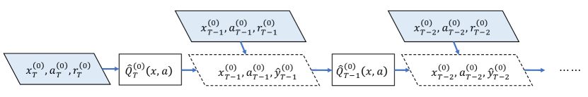
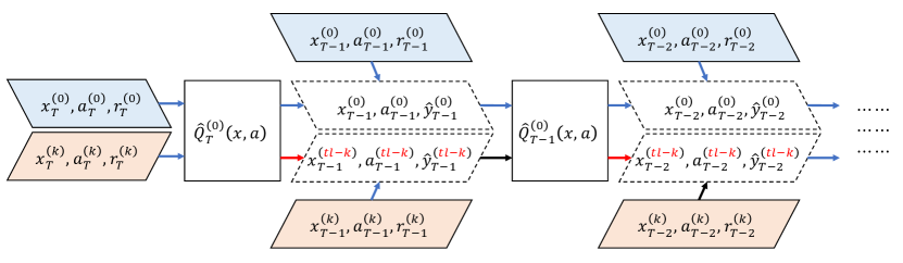
Figure 1: Illustration of single-task $Q$-learning (top) and transferred $Q$-learning (bottom). Single-task methods only use data in blue blocks and do not contain the $k$-th source data in orange blocks. The re-targeting step is highlighted in red.

3.2 Offline stage-to-stage transfer

To leverage the source data for offline RL tasks, we propose a transferred $Q$-learning algorithm, which is based on a commonly-used backward recursive approach in both machine learning and dynamic treatment regimes. The algorithm is summarized in Algorithm 1, where $\boldsymbol{X}_{t}^{(k)}\in\mathbb{R}^{n_{k}\times p}$ denote the design matrix for the $k$-th task at stage $t$ whose $i$-th row is $(\boldsymbol{x}_{t,i}^{(k)})^{\top}$ and $\boldsymbol{W}_{t}^{(k)}$ is a ${n_{k}\times(2p)}$ matrix whose $i$-th row is $((\boldsymbol{x}_{t,i}^{(k)})^{\top},a_{t,i}^{(k)}(\boldsymbol{x}_{t,i}^{(k)})^{\top})$.

Now we give a more detailed explanation of the algorithm (see Algorithm 1). First, starting from the final stage $T$, we have full observations of $\{\boldsymbol{x}_{T,i}^{(k)},a_{T,i}^{(k)},y_{T,i}^{(k)}\}_{i\in[n_{k}]}$ for each task and hence supervised TL algorithms can be directly applied to obtain the target parameter $\widehat{\boldsymbol{\theta}}_{T}$. Then, moving backwardly to stage $t=T-1,\cdots,1$, we calculate the pseudo response $y_{t,i}^{(0)}$ in (9) using $\widehat{\boldsymbol{\theta}}_{t+1}$, which estimates the full observations for the $Q$-function at stage $t$ for the target task. To borrow information from the source data, we calculate the re-targeted pseudo response $y_{t,i}^{(tl-k)}$ in (15) using $\widehat{\boldsymbol{\theta}}_{t+1}$, which estimates the full observations for each source task. Hence any chosen supervised TL algorithm can be applied to the target pseudo data $y_{t,i}^{(0)}$, together with the source pseudo data $y_{t,i}^{(tl-k)}$, $k\in[K]$, to obtain the target parameter $\widehat{\boldsymbol{\theta}}_{t}$. Here, we employ the Trans-Lasso algorithm (Li et al., 2020a) – a representation of the transferred linear regression method – for its simplicity and rate optimal properties.

Input : Target data $\{\boldsymbol{X}^{(0)}_{t},\boldsymbol{a}^{(0)}_{t},\boldsymbol{r}_{t}^{(0)}\}_{t\in[T]}$, source data $\{\{\boldsymbol{X}_{t}^{(k)},\boldsymbol{a}^{(k)}_{t},\boldsymbol{r}_{t}^{(k)}\}_{k=1}^{K}\}_{t\in[T]}$, and discount factor $\gamma$.

Output : $\{\widehat{\boldsymbol{\theta}}_{t}\}_{t=1}^{T}$.

1

2Initialization: $\widehat{\boldsymbol{\theta}}_{T+1}=0$.

3for $t=T,\dots,1$ do

4      

5      Create pseudo-outcome which promotes similarity: $\widehat{\boldsymbol{y}}^{(tl-k)}_{t}=\boldsymbol{r}_{t}^{(k)}+\gamma(\boldsymbol{X}^{(k)}_{t+1}\widehat{\boldsymbol{\beta}}_{t+1}+|\boldsymbol{X}^{(k)}_{t+1}\widehat{\boldsymbol{\psi}}_{t+1}|)$, $k=1,\dots,K$; $\widehat{\boldsymbol{y}}^{(0)}_{t}=\boldsymbol{r}_{t}^{(0)}+\gamma(\boldsymbol{X}^{(0)}_{t+1}\widehat{\boldsymbol{\beta}}_{t+1}+|\boldsymbol{X}^{(0)}_{t+1}\widehat{\boldsymbol{\psi}}_{t+1}|)$.

6      Apply the transfer learning algorithm for supervised regression:

$$\widehat{\boldsymbol{b}}_{t} =\operatorname{argmin}_{\boldsymbol{w}\in\mathbb{R}^{p}}\left\{\sum_{k=1}^{K}\|\widehat{\boldsymbol{y}}_{t}^{(tl-k)}-\boldsymbol{W}_{t}^{(k)}\boldsymbol{b}\|_{2}^{2}+\lambda_{\mathrm{src}}\|\boldsymbol{b}\|_{1}\right\}.$$

$$\widehat{\boldsymbol{\delta}}_{t} =\operatorname{argmin}_{\boldsymbol{\delta}\in\mathbb{R}^{p}}\left\{\|\widehat{\boldsymbol{y}}_{t}^{(0)}-\boldsymbol{W}^{(0)}_{t}(\boldsymbol{\delta}+\widehat{\boldsymbol{b}}_{t})\|_{2}^{2}+\lambda_{0}\|\boldsymbol{\delta}\|_{1}\right\}.$$

Threshold $\widehat{\boldsymbol{\delta}}_{t}$ such that $(\check{\boldsymbol{\delta}}_{t})_{j}=(\widehat{\boldsymbol{\delta}}_{t})_{j}\mathbbm{1}(|(\widehat{\boldsymbol{\delta}}_{t})_{j}|\geq\lambda_{0})$. Threshold $\widehat{\boldsymbol{b}}_{t}$ such that $(\check{\boldsymbol{b}}_{t})_{j}=(\widehat{\boldsymbol{b}}_{t})_{j}\mathbbm{1}(|(\widehat{\boldsymbol{b}}_{t})_{j}|\geq\lambda_{\mathrm{src}})$.

7      Output $\widehat{\boldsymbol{\theta}}_{t}=\check{\boldsymbol{b}}_{t}+\check{\boldsymbol{\delta}}_{t}$.

Algorithm 1 Transferred $Q$-learning algorithm

We can see that the proposed method enables information transfer in two different forms at every step corresponding to Figure 1 (lower panel). First, the estimated response for the target model, $\widehat{\boldsymbol{y}}_{t,i}^{(0)}$, integrates the information in different tasks from the previous step since it is based on the transfer learning $\widehat{\boldsymbol{\theta}}_{t+1}$. As a result, the current-step estimator $\widehat{}\boldsymbol{\theta}_{t}$ benefits as well since the current response estimation $\widehat{\boldsymbol{y}}_{t,i}^{(0)}$ has smaller error than its single task counterpart. Second, when estimating $\boldsymbol{\theta}_{t}$, we apply a transfer learning algorithm for supervised regression, which also borrows information from $t$-th stage of source studies, i.e., the information in $\{\boldsymbol{r}_{t,i}^{(k)}\}_{k=1}^{K}$.

The second step of Algorithm 1 is closely related to transfer learning in supervised regressions. For example, Lounici et al. (2009) considered transfers across multiple high-dimensional sparse models under an assumption that the support of all the regression coefficients are the same. Bastani (2021) studied estimation and prediction in high-dimensional linear models with one informative source study where the sample size of the source study is larger than the number of covariates. Li et al. (2020a) proposes a method for high-dimensional linear regression based on transfer learning with minimax optimality. Our proposal originates from Li et al. (2020a) and further conquers the unique challenges in $Q$-learning. In fact, other supervised TL methods can be leveraged here. For example, Tripuraneni et al. (2020) proposes a transfer learning method assuming a low-rank structure of the coefficient vectors for different tasks. And this method can also be used in Algorithm 1 at each stage with estimated data $(\boldsymbol{X}^{(k)}_{t},\boldsymbol{a}_{t}^{(k)},\widehat{\boldsymbol{y}}_{t}^{(tl-k)})$. The last thresholding step in line 6 of the Algorithm 1 produces sparse estimators without inflating estimation errors. The sparse estimators, $\check{\boldsymbol{b}}_{t}$ and $\check{\boldsymbol{\delta}}_{t}$ have desirable prediction errors for general sub-Gaussian designs, which lead to desired convergence rate. The multi-stage $Q$-learning has complex dependencies across stages and they make the restricted eigenvalue conditions suspicious without thresholding.

As a summary, transferred $Q$-learning differs from transferred supervised learning in the following two aspects. First, $Q$-learning is a multi-stage model and for the stage $t$ for $t<T$, we only have partial observations $\boldsymbol{r}^{(k)}_{t,i}$ and the estimated full responses $\widehat{\boldsymbol{y}}^{(tl-k)}_{t,i}$ contain measurement errors. The proposed transferred $Q$-learning enables the benefit of transfer to be shared across stages. Second, the estimated full responses $\widehat{\boldsymbol{y}}^{(tl-k)}_{t,i}$ is nonlinear in the estimated parameters $\widehat{\boldsymbol{\theta}}_{t+1}$. Our proposal generalizes the existing Trans-Lasso to deal with proximal responses rather than the direct observations of responses.

3.3 Offline-to-Online transfer

In this subsection, we introduce the offline-to-online transferred $Q$-learning algorithm. In this context, transfer learning can provide an efficient way to leverage the offline data, including demonstrations for the target task, suboptimal policies and demonstrations for the source tasks. Algorithm 2 presents the online transferred $Q$-learning framework based on exploration and then commit (ETC) paradigm.

Input : Offline data: $\{\{\boldsymbol{X}_{t}^{(k)},\boldsymbol{a}_{t}^{(k)},\boldsymbol{r}_{t}^{(k)}\}_{k=1}^{K}\}_{t\in[T]}$.

Exploration phase length $n_{e}$, an exploration policy $\pi_{e}$.

Output : Online actions $\{\widehat{a}^{(0)}_{t,i}\}_{t\in[T]}$,  $i=1,\dots$

1

2Initialization: $\widehat{\boldsymbol{\theta}}_{T+1}=0$.

3 # exploration phase

4for $i=1,\dots,n_{e}$ do

5       for $t=1,\dots,T$ do

6             Take action $a_{t,i}^{(0)}=\pi_{e}(\cdot|\boldsymbol{x}^{(0)}_{t,i})$ and observe $r^{(0)}_{t,i}$ and $\boldsymbol{x}^{(0)}_{t+1,i}$.

7      

8 # learning phase

9Run Algorithm 1 with target data $\{\{\boldsymbol{x}^{(0)}_{t,i},a^{(0)}_{t,i},r^{(0)}_{t,i}\}_{i=1}^{n_{e}}\}_{t\in[T]}$ and offline source data $\{\{\boldsymbol{X}_{t}^{(k)},\boldsymbol{a}^{(k)}_{t},\boldsymbol{r}_{t}^{(k)}\}_{k=1}^{K}\}_{t\in[T]}$. Output $\{\widehat{\boldsymbol{\theta}}_{t}\}_{t=1}^{T}$.

10 # exploitation phase

11for $i=n_{e}+1,\dots,$ do

12       for $t=1,\dots,T$ do

13             Take greedy action $\widehat{a}_{t,i}=\operatorname*{arg\,max}_{a\in\{-1,1\}}\widehat{Q}(\boldsymbol{x}^{(0)}_{t,i},a;\widehat{\boldsymbol{\theta}}_{t})$ and transit to $\boldsymbol{x}^{(0)}_{t+1,i}$.

14      

Algorithm 2 Online RL with transfer from offline data

Algorithm 2 first generates $n_{e}$ trajectories from the target task in the exploration phase. Then in the learning phase, Algorithm 1 is called to combine the target data with the offline source data to estimate the target parameters. Lastly in the exploitation phase, it conducts greedy action to maximize the estimated $Q$-function at each stage afterwards. The longer the exploration phase, the larger the regret since the estimated optimal policy is not employed in the exploration phase. We will show in theory that $n_{e}$ can be set much smaller by leveraging offline data under certain conditions. Specifically, it suffices to take $n_{e}\geq c\log p$ in Algorithm 2 when having large amount of offline data. In contrast, without offline data, we show that one need to take $n_{e}\geq cs\log p$. This is because one can learn a near-optimal policy based on the offline data when the offline tasks are sufficiently similar to the target task.

4 Theoretical results

In this section, we provide rigorous error and regret analyses of both offline and online transferred $Q$-learning under the similarity characterization (11). Under such similarity, the parameter space we consider is

$$\Omega(s,h)=\left\{(\boldsymbol{\theta}_{t},\boldsymbol{\delta}^{(1)}_{t},\dots,\boldsymbol{\delta}^{(K)}_{t}),t\in[T]:~{}\max_{t\in[T]}\|\boldsymbol{\theta}_{t}\|_{0}\leq s,\max_{t\in[T],k\in[K]}\|\boldsymbol{\delta}_{t}^{(k)}\|_{1}\leq h\right\}.$$

We write $N_{\mathrm{src}}=\sum_{k=1}^{K}n_{k}$ as the total number of trajectories from the source tasks.

Assumption 1 (Conditions on the design).

For $k=0,\dots,K$ and $t=1,\dots,T$, $\boldsymbol{x}_{t,i}^{(k)}$ are independent sub-Gaussian with mean zero. For $(\boldsymbol{w}_{t,i}^{(k)})^{\top}=[(\boldsymbol{x}_{t,i}^{(k)})^{\top},a_{t,i}^{(k)}(\boldsymbol{x}_{t,i}^{(k)})^{\top}]$, the covariance matrices $\boldsymbol{\Sigma}^{(k)}_{t}=\mathbbm{E}[\boldsymbol{w}_{t,i}^{(k)}(\boldsymbol{w}_{t,i}^{(k)})^{\top}]$ is positive definite with bounded eigenvalues, $t=1,\dots,T$, $k=1,\dots,K$. Moreover,

$$\max_{t\in[T]}\max_{k\in[K]}\left\lVert\boldsymbol{\Sigma}^{(k)}_{t}(\boldsymbol{\Sigma}^{(0)}_{t})^{-1}-I_{2p}\right\rVert_{\infty,1}\leq C_{\Sigma}<1.$$ (16)

Assumption 2 (Conditions on the noises).

For $y^{(tl-k)}_{t,i}$ defined in (12), the residuals $y^{(0)}_{t,i}-\mathbb{E}[y^{(0)}_{t,i}|\boldsymbol{x}_{t,i}^{(0)},a_{t,i}^{(0)}]$ and $y^{(tl-k)}_{t,i}-\mathbb{E}[y^{(tl-k)}_{t,i}|\boldsymbol{x}_{t,i}^{(k)},a_{t,i}^{(k)}]$, $k\in[K]$, are independent sub-Gaussian random variables.

Assumption 1 requires sub-Gaussian designs for all the tasks. The positive definiteness of $\boldsymbol{\Sigma}_{t}^{(k)}$ assumes regularity of the covariance of $\boldsymbol{x}_{t,i}^{(k)}$ but also requires $a_{t,i}^{(k)}$ has constant variance across samples. Moreover, we require in (16) that the covariance matrices for the source and target tasks are sufficiently similar. Assumption 2 requires sub-Gaussian noises in the observed reward at each stage.

4.1 Convergence rate of Algorithm 1

We provide theoretical guarantees for the offline stage-to-stage transfer in this subsection. Theorem 1 establishes the convergence rate for $\{\widehat{\boldsymbol{\theta}}_{t}\}_{t\in[T]}$ in this setting.

Theorem 1 (Convergence rate of Algorithm 1).

Suppose that Assumptions 1 and 2 hold and $\log p\leq c_{0}n_{0}$ for some constant $c_{0}>0$. We take the tuning parameters to be

$$\lambda_{\mathrm{src}}=c_{1}\sqrt{\frac{\log p}{N_{\mathrm{src}}}}+c_{1}\sqrt{\frac{h}{s}}\left(\frac{\log p}{n_{0}}\right)^{1/4}~{}\text{and}~{}\lambda_{0}=c_{1}\sqrt{\frac{\log p}{n_{0}}}.$$

Under the sample size condition that $s\sqrt{\log p/N_{\mathrm{src}}}+h+sh\sqrt{\log p/n_{0}}\leq C$, for any $t=1,\dots,T$, we have

$$\frac{1}{n_{0}}\left\lVert\boldsymbol{W}^{(0)}_{t}(\widehat{\boldsymbol{\theta}}_{t}-\boldsymbol{\theta}_{t})\right\rVert_{2}^{2}\vee\left\lVert\widehat{\boldsymbol{\theta}}_{t}-\boldsymbol{\theta}_{t}\right\rVert_{2}^{2}\lesssim\left\lVert\widehat{\boldsymbol{\theta}}_{t+1}-\boldsymbol{\theta}_{t+1}\right\rVert_{2}^{2}+\frac{s\log p}{N_{\mathrm{src}}}+h\sqrt{\frac{\log p}{n_{0}}}.$$

with probability at least $1-\exp(-c_{2}\log p)$.

Theorem 1 establishes the estimation accuracy of the target $Q$-function at each stage. The rate for the final stage ($t=T$) is the minimax optimal rate in supervised regression with transfer learning (Li et al., 2020b) since the final-stage reward equals the value of the state-action pair. For the $t$-th stage ($t<T$), the estimation error from $\widehat{\boldsymbol{\theta}}_{t+1}-\boldsymbol{\theta}_{t+1}$ accumulates, as a consequence of using pseudo-outcomes. Thus, empirically one may expect that the estimation errors become larger in the earlier stages, even though the convergence rate of each stage are the same. In the upper bound, the sparsity $s$ of the target parameter is weighted with $1/N_{\mathrm{src}}$ and the maximum sparsity $h$ of the contrast vectors is weighted with $1/\sqrt{n_{0}}$. This shows the improvement of transfer learning, where the $s$-sparse component is learned based on all the studies but the task-specific contrast vectors can only be identified based on the target study with $n_{0}$ samples. When the similarity is sufficiently high, then $h\ll s$ and transfer learning can lead to improvements in this case. In the theorem, we our choice of $\lambda_{\mathrm{src}}$ depends on the unknown $h/s$, which is for a convenient proof of desirable convergence rate. When $h/s\ll\sqrt{n_{0}\log p}/N_{\mathrm{src}}$, $\lambda_{\mathrm{src}}\asymp\sqrt{\log p/N_{\mathrm{src}}}$. In practice, $\lambda_{\mathrm{src}}$ can be chosen by cross-validation.

Remark 2 (Convergence rate of single-task $Q$-learning).

Let $\widehat{\boldsymbol{\theta}}_{t}^{(st)}$, $t\in[T]$, be the single-task $Q$-learning estimator studied in Song et al. (2015). For any $t=1,\dots,T$,

$$\|\widehat{\boldsymbol{\theta}}_{t}^{(st)}-\boldsymbol{\theta}_{t}\|_{2}^{2}\lesssim\|\widehat{\boldsymbol{\theta}}^{(st)}_{t+1}-\boldsymbol{\theta}_{t+1}\|_{2}^{2}+\frac{s\log p}{n_{0}}.$$

For the final stage, the transfer learning estimator $\widehat{\boldsymbol{\theta}}_{T}$ has faster convergence rate than the single-task estimator $\widehat{\boldsymbol{\theta}}_{T}^{(st)}$ as long as $N_{\mathrm{src}}\gg n_{0}$ and $h\ll s\sqrt{\log p/n_{0}}$. Furthermore, the convergence rate of $\widehat{\boldsymbol{\theta}}_{T}$ is minimax optimal in the parameter space of interest. For the $t$-th stage for $t<T$, the gain of transfer learning has two aspects. The first is the error inherited from the next stage, $\|\widehat{\boldsymbol{\theta}}_{t+1}-\boldsymbol{\theta}_{t+1}\|_{2}^{2}$, which is smaller than its single-task counterpart $\|\widehat{\boldsymbol{\theta}}_{t+1}^{(st)}-\boldsymbol{\theta}_{t+1}\|_{2}^{2}$. The second gain comes from aggregating the data at the current stage.

4.2 Regret bound of offline-to-online transferred $Q$-learning

In this subsection, we provide theoretical guarantees for the online Algorithm 2 with knowledge transferred from offline data. In the online setting, the learner aims to minimize the cumulative regret that measures the expected loss of following the estimated optimal policy instead of the oracle optimal policy. Mathematically, the cumulative regret over $T$ episodes is defined as

$${\rm Regret}_{NT}=\sum_{i=1}^{N}\gamma^{t}\sum_{t=1}^{T}\left(\mathbb{E}[r_{t,i}^{(0)}|\boldsymbol{x}^{(0)}_{t,i},a^{*}_{t,i}]-\mathbb{E}[r_{t,i}^{(0)}|\boldsymbol{x}^{(0)}_{t,i},\widehat{a}^{(0)}_{t,i}]\right),$$ (17)

where the estimated optimal policy is $\widehat{a}_{t,i}^{(0)}=\operatorname*{arg\,max}_{a^{\prime}\in\{-1,1\}}Q(\boldsymbol{x}_{t,i}^{(0)},a^{\prime};\widehat{\boldsymbol{\theta}}_{t})$ and the oracle optimal policy is $a^{*}_{t,i}=\operatorname*{arg\,max}_{a^{\prime}\in\{-1,1\}}Q(\boldsymbol{x}_{t,i}^{(0)},a^{\prime};\boldsymbol{\theta}_{t})$. Under the linear $Q$-function (6), they can be further simplified to

$$\widehat{a}_{t,i}^{(0)}=sgn((\boldsymbol{x}^{(0)}_{t,i})^{\top}\widehat{\boldsymbol{\psi}}_{t}),\quad\text{and}\quad a^{*}_{t,i}=sgn((\boldsymbol{x}^{(0)}_{t,i})^{\top}\boldsymbol{\psi}_{t}),$$

where $sgn(\cdot)$ is the sign function. The regret bound of online learning with offline transfer is given in Theorem 2.

Theorem 2 (Cumulative regret of Algorithm 2 after $T$ rounds).

Suppose that Assumption 1 - 2 hold and $s\sqrt{\log p/N_{\mathrm{src}}}+h\leq C$, $n_{e}\gtrsim s^{2}h^{2}\log p+\log p$. We take tuning parameters to be

$$\lambda_{\mathrm{src}}=\sqrt{\frac{\log p}{N_{\mathrm{src}}}}+\sqrt{\frac{h}{s}}\left(\frac{\log p}{n_{e}}\right)^{1/4}~{}~{}\text{and}~{}~{}\lambda_{0}=\sqrt{\frac{\log p}{n_{e}}}.$$

For any $N>n_{e}$,

$${\rm Regret}_{NT}\lesssim\frac{n_{e}\gamma}{1-\gamma}+(N-n_{e})\left(\sqrt{\frac{s\log p}{N_{\mathrm{src}}}}+h^{1/2}\left(\frac{\log p}{n_{e}}\right)^{1/4}\right)$$ (18)

with probability at least $1-\exp(-c_{1}\log p)$.

We now find the optimal choice of $n_{e}$, which minimizes the RHS of (18). To simplify the analysis, we parameterize $h=N_{\mathrm{src}}^{-\alpha}$ for some $\alpha\geq 0$. In the supplementary files, we show that if we take

$$n_{e}\asymp\max\left\{\frac{N^{4/5}(\log p)^{1/5}}{N_{\mathrm{src}}^{2\alpha/5}},\frac{s^{2}\log p}{N_{\mathrm{src}}^{2\alpha}}\right\},$$

then with probability at least $1-\exp(-c_{1}\log p)$

$${\rm Regret}_{NT}\lesssim\max\left\{\frac{N^{4/5}(\log p)^{1/5}}{N_{\mathrm{src}}^{2\alpha/5}},\frac{s^{2}\log p}{N_{\mathrm{src}}^{2\alpha}}\right\}+N\sqrt{\frac{s\log p}{N_{\mathrm{src}}}}.$$ (19)

We see that larger the $N_{\mathrm{src}}$, i.e., more source data, smaller the cumulative regret; and the larger the value of $\alpha$, i.e., higher the similarity, smaller the cumulative regret.

Remark 3 (Cumulative regret of single-task $Q$-learning).

Without offline data, we denote the estimated optimal policy by $\widehat{a}^{(st)}$. It is easy to show that for $n_{e}\gg(s\log p)^{2}$, then with probability at least $1-\exp(-c_{1}\log p)$,

$${\rm Regret}_{NT}^{(st)}\lesssim\frac{n_{e}\gamma}{1-\gamma}+(N-n_{e})\sqrt{\frac{s\log p}{n_{e}}}.$$ (20)

with probability at least $1-\exp(-c_{1}\log p)$. If we take $n_{e}\asymp N^{2/3}(s\log p)^{1/3}\vee(s\log p)^{2}$, then

$${\rm Regret}_{NT}^{(st)}\lesssim N^{2/3}(s\log p)^{1/3}+(s\log p)^{2}$$ (21)

with probability at least $1-\exp(-c_{1}\log p)$.

Comparing (18) with (20), we see that the cumulative regret of transferred $Q$-learning is always smaller when $h=o(s\sqrt{\log p/n_{e}})$. Comparing (19) with (21), we see that as long as $N_{\mathrm{src}}>N^{1/(3\alpha)}+N^{2/3}$, the regret of transfer learning policy is always no larger than the single-task policy. This comparison further implies that if $N$ is very large, then the optimal choice of $n_{e}$ can be larger than $N_{\mathrm{src}}$. In this case, transfer learning may not have significant improvement and it suffices to consider single-task $Q$-learning.

5 Numerical Studies

In this section, we demonstrate the advantage of the proposed transferred Q-learning algorithm on synthetic and real data sets. Code and implementation details for this section are available online at https://github.com/ElynnCC/TransferredQLearning.

5.1 Two-stage MDP with analytical optimal $Q^{*}$ function

We first consider a simple MDP model which has an analytical form for the optimal $Q$ function. In such a setting we can explicitly compare the estimated $Q$ function with the ground truth. The generative model is designed based on those in Chakraborty et al. (2010) and Song et al. (2015). The underlying model is a two-stage MDP with two possible actions ${\cal A}=\left\{-1,1\right\}$ and two states ${\cal S}=\left\{-1,1\right\}$. The binary states $S_{t}$’s and the binary treatment $A_{t}$ are generated as follows:

$$\Pr\left(S_{1}=-1\right)=\Pr\left(S_{0}=1\right)=0.5,$$

$$\Pr\left(A_{t}=-1\right)=\Pr\left(A_{t}=1\right)=0.5,\quad t=1,2,$$

$$\Pr\left(S_{2}|S_{1},A_{1}\right)=1-\Pr\left(S_{2}|S_{1},A_{1}\right)={\rm expit}\left(b_{1}S_{1}+b_{2}A_{1}\right),$$

where ${\rm expit}\left(x\right)=\exp\left(x\right)/\left(1+\exp\left(x\right)\right)$. The immediate reward $R_{1}=0$ and $R_{2}$ is given by

$$R_{2}=\kappa_{1}+\kappa_{2}S_{1}+\kappa_{3}A_{1}+\kappa_{4}S_{1}A_{1}+\kappa_{5}A_{2}+\kappa_{6}S_{2}A_{2}+\kappa_{7}A_{1}A_{2}+\varepsilon_{2},$$

where $\varepsilon_{2}\sim{\cal N}\left(0,1\right)$. Under this setting, the true $Q$ functions for time $t=1,2$ are

$$Q_{2}\left(S_{2},A_{2};\boldsymbol{\theta}_{2}\right) =\theta_{2,1}+\theta_{2,2}S_{1}+\theta_{2,3}A_{1}+\theta_{2,4}S_{1}A_{1}+\theta_{2,5}A_{2}+\theta_{2,6}S_{2}A_{2}+\theta_{2,7}A_{1}A_{2}$$ (22)

$$Q_{1}\left(S_{1},A_{1};\boldsymbol{\theta}_{1}\right) =\theta_{1,1}+\theta_{1,2}S_{1}+\theta_{1,3}A_{1}+\theta_{1,4}S_{1}A_{1},$$

where the true coefficients $\boldsymbol{\theta}_{t}$ are explicitly functions of $b_{1}$, $b_{2}$, $\kappa_{1},\dots,\kappa_{7}$ given in (LABEL:eqn:true-q-theta) in the supplemental material. At each state, the observed covariates $X_{t}\in\mathbb{R}^{p}$, $p=100$, consist of first eight elements $1$, $S_{1}$, $A_{1}$, $S_{1}A_{1}$, $A_{2}$, $S_{2}$, $S_{2}A_{2}$, $A_{1}A_{2}$ and the remaining elements that are randomly sampled from standard normal.

We consider transfer between two different but similar MDPs from the above model. The target and source MDPs are different in the coefficients $\kappa$’s and therefore $\theta$’s in (22). Specifically, we set $\theta_{2,j}=1$, $1\leq j\leq 7$ for the target MDP. The second-stage coefficients of the source task are the same except that the second element $\theta_{2,2}^{(1)}=1.2$. Therefore, according to equation (LABEL:eqn:true-q-theta) in the supplemental material, the true coefficients of stage-one $Q$ functions are $\theta_{1,1},\theta_{1,2},\theta_{1,3},\theta_{1,4}\approx 2.69,1.19,1.69,1.19$ for the target MDP, and $\theta_{1,1}^{(1)},\theta_{1,2}^{(1)},\theta_{1,3}^{(1)},\theta_{1,4}^{(1)}\approx 2.69,1.39,1.69,1.19$ for the source MDP. In summary, the true $Q_{1}$ functions of the target and source MDPs are different only in $\theta_{1,2}$ and the $Q_{2}$ functions are different only in $\theta_{2,2}$. The coefficients of rest of the elements in $X_{t}$ are all set as zero. We generate trajectories of the form $\left(\boldsymbol{x}_{1,i},a_{1,i},r_{1,i},\boldsymbol{x}_{2,i},a_{2,i},r_{2,i}\right)$ from both target and source MDPs. The target task consists of $n_{0}$ trajectories while the source task consists of $n_{1}$ trajectories.

We compare $\left\lVert\widehat{}\boldsymbol{\theta}_{t}-\boldsymbol{\theta}_{t}\right\rVert_{2}^{2}$, $t=1,2$, with or without transfer under combinations of $n_{0}$ and $n_{\mathrm{src}}=n_{1}$. The boxplots are shown in Figure 2. We also generate a new dataset and compare predicted $\widehat{Q}^{*}(\boldsymbol{x},a)$ obtained by transferred $Q$ learning and its vanilla counterpart. The boxplots of $\left\lvert\widehat{Q}^{*}(\boldsymbol{x},a)-Q^{*}(\boldsymbol{x},a)\right\rvert/\left\lvert Q^{*}(\boldsymbol{x},a)\right\rvert$ (averaged over all state-action pairs in the new dataset) are presented in Figure 3. It is clear that transferred $Q$-learning performs much better than the vanilla $Q$-learning without transfer in terms of both coefficient estimation and prediction. The advantage is more prominent in earlier stages since the transfer benefit in the latter stage positively cascade to the earlier stages through the second term in (12).

Table 1 compares the frequency of correct optimal actions chosen by single-task $Q$-learning and Transferred $Q$-learning with the new dataeset. We observe that Transferred $Q$-learning achieves higher accuracy in choosing the optimal actions across all combinations of $n_{0}$ and $n_{1}$, which are the number of trajectories of the target task and the source task, respectively. The amplitude of accuracy increase is higher when $n_{0}$ is small. This again shows the advantage of Transferred $Q$-learning, especially when the number of trajectories of the target task is small.

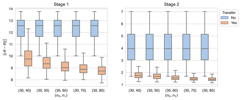
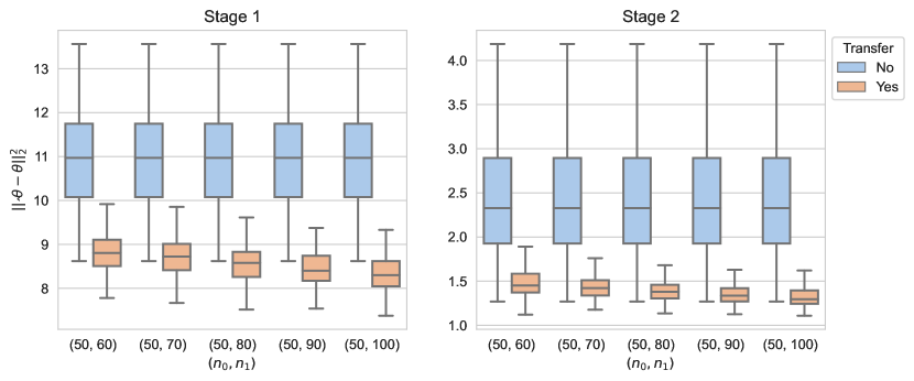
Figure 2: Comparison of the estimated coefficients of the optimal $Q$ function. The $y$-axis represents $\left\lVert\widehat{}\boldsymbol{\theta}_{t}-\boldsymbol{\theta}_{t}\right\rVert_{2}^{2}$ for $t=1$ (left) and $t=2$ (right). The dimension is $p=100$ and sparsity $s=7$.

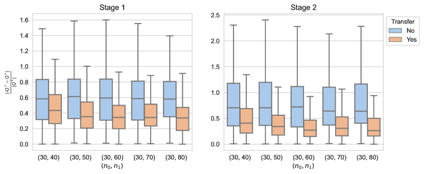
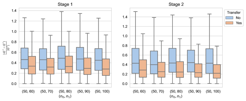
Figure 3: Comparison of the prediction of the optimal $Q$ function with different sample size configurations. The $y$-axis represents $\left\lvert\widehat{Q}^{*}-Q^{*}\right\rvert/\left\lvert Q^{*}\right\rvert$. The dimension is $p=100$ and sparsity $s=7$.

Table 1: The frequency of correct optimal actions. The comparison is between the optimal action $A^{*,(st)}$ chosen by single-task $Q$-learning and the optimal action $A^{*,(tl)}$ chosen by Transferred $Q$-learning. We consider different combinations of $n_{0}=30,50,70$ and $n_{1}=n_{0}+10,\,\cdots,n_{0}+50$, where $n_{0}$ and $n_{1}$ denote the number of trajectories of the target task and the source task, respectively.

$n_{0}$	$A^{*,(st)}$	$A^{*,(tl)}$ with different $n_{1}$
		$n_{0}+10$	$n_{0}+20$	$n_{0}+30$	$n_{0}+40$	$n_{0}+50$
30	0.555	0.965	0.985	0.990	0.970	0.985
50	0.860	0.990	0.995	1.000	1.000	1.000
70	0.905	1	1	1	1	1

5.2 Offline to online transfer

In this section, we study the empirical performance of online transferred $Q$-learning using an offline source dataset. The generative MDP is the same as that defined in (22). We have access to an offline source dataset of trajectories $\left(X_{1},A_{1},R_{1},X_{2},A_{2},R_{2}\right)$ generated from an MDP with $\theta_{2j}^{(1)}=\kappa_{j}^{(1)}=1$, $1\leq j\leq 3$, $5\leq j\leq 7$ and $\theta_{2j}^{(1)}=\kappa_{j}^{(1)}=2$, $j=4$. The online target RL task is modeled by an MDP with $\theta_{2j}^{(1)}=\kappa_{j}^{(1)}=1$, $1\leq j\leq 7$. The dimension of covariates is $p=100$.

We first study the cumulative regrets of transferred and vanilla $Q$-learning with different lengths of exploration, $n_{e}\in\left\{1,2,\cdots,20\right\}$. The size of the offline source dataset is $n_{1}=100$. At the exploration stage, $n_{e}$ trajectories are generated by random actions. The coefficients $\widehat{}\boldsymbol{\theta}_{t}$ are estimated using $Q$-learning with or without transfer. The average cumulative regret at the exploitation stage versus different length of exploration are presented in Figure 4 (a). The length of exploitation stage is $100$. For each $n_{e}$, the mean of the cumulative regret at exploitation stage is reported since the values of $\widehat{}\boldsymbol{\theta}_{t}^{(0)}$ are not updated during exploitation stage. We observe that under the condition that $h\ll s\sqrt{\log p/n_{\mathrm{ex}}}$, the regret of transferred $Q$-learning is much smaller than that of the vanilla $Q$-learning, which is consistent with the result in Theorem 2. Since Algorithm 2 is of the explore-then-commit (ETC) type, the advantage of transferred $Q$ learning shown in the left panel of Figure 4 can be viewed as the jumpstart improvement – one of the three main objectives of transfer learning defined in Langley (2006) and Taylor and Stone (2009).

We also empirically study the cumulative regret of online $Q$-learning where the values of $\widehat{}\boldsymbol{\theta}_{1}$ and $\widehat{}\boldsymbol{\theta}_{2}$ are updated during the exploitation stage. This phase-based ETC online $Q$-learning algorithm is a natural extension of Algorithm 2 and it goes as follows. At the first phase, vanilla $Q$-learning initializes $\widehat{}\boldsymbol{\theta}_{1}$ and $\widehat{}\boldsymbol{\theta}_{2}$ as zero, while transferred $Q$-learning initializes with $\widehat{}\boldsymbol{\theta}_{1}$ and $\widehat{}\boldsymbol{\theta}_{2}$ that are estimated using offline trajectories from the source task. Then at each phase, a batch of $100$ trajectories are generated using greedy actions based on estimated $\widehat{}\boldsymbol{\theta}_{1}$ and $\widehat{}\boldsymbol{\theta}_{2}$. Using the extra generated trajectories at the current phase, the values $\widehat{}\boldsymbol{\theta}_{1}$ and $\widehat{}\boldsymbol{\theta}_{2}$ are updated and will be used to generate greedy actions for the next phase. Right panel of Figure 4 shows the mean of cumulative regret as phases proceed online. It shows all three main advantages of transferred learning, namely, jumpstart, learning speed, and asymptotic improvements (Langley, 2006; Taylor and Stone, 2009).

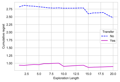
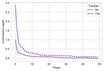
Figure 4: Cumulative regret of online $Q$-learning with or without transfer. Left panel: The explore-then-commit (ETC) online $Q$-learning; Right panel: phase-based ETC online $Q$-learning with parameter updates.

5.3 Medical data application: Mimic-iii Sepsis cohort

In this section, we illustrate an application of the transferred $Q$-learning in the Medical Information Mart for Intensive Care version III (MIMIC-III) Database (Johnson et al., 2016), which is a freely available source of de-identified critical care data from 2001 – 2012 in six ICUs at a Boston teaching hospital.

We consider a cohort of sepsis patients, following the same data processing procedure as that in Komorowski et al. (2018). Each patient in the cohort is characterized by a set of 47 variables, including demographics, Elixhauser premorbid status, vital signs, and laboratory values. Patients’ data were coded as multidimensional discrete time series $\boldsymbol{x}_{i,t}\in\mathbb{R}^{47}$ for $1\leq i\leq N$ and $1\leq t\leq T_{i}$ with 4-hour time steps. The actions of interests are the total volume of intravenous (IV) fluids and maximum dose of vasopressors administrated over each 4-hour period. We discretize two actions into three levels (i.e. low, medium, and high), respectively. In our setting, the low-level corresponds to level 1 - 2, the medium-level corresponds to level 3 and the high-level corresponds to level 4 - 5 in Komorowski et al. (2018). The combination of the two drugs makes $M=3\times 3=9$ possible actions in total. The final processed dataset contains 20943 unique adult ICU admissions, among which 11704 (55.88%) are female (0) and 9239 (44.11%) are male (1).

The reward signal is important and is crafted carefully in real applications. For the final reward, we follow Komorowski et al. (2018) and use hospital mortality or 90-day mortality. Specifically, when a patient survived after 90 days out of hospital, a positive reward was released at the end of each patient’s trajectory; a negative reward was issued if the patient died in hospital or within 90 days out of hospital. In our dataset, the mortality rate is 24.21% for female and 22.71% for male. For the intermediate rewards, we follow Prasad et al. (2017) and associates reward to the health measurement of a patient. The detailed description of the data pre-processing is presented in Section LABEL:appen:mimic-iii of the supplemental material.

The trajectory horizons are different in the dataset, with the maximum being 20 and minimum being 1. We use 20 as the total length of horizon. The trajectories are aligned at the last steps while allowing the starting steps vary. For examples, the trajectories with length 20 start at step $1$ while the trajectories with length 10 start at step $11$. But they all end at step 20. We adopt this method because the distribution of final status are similar across trajectories. Figure 5 presents the mortality rates of different lengths. We see that, while the numbers of trajectories differ a lot, the mortality rates do not vary much across trajectories with different horizons. On the contrary, the starting status of patients may be very different. The one with trajectory length $20$ may be in a worse status and needs first $10$ steps to reach the status similar to the starting status of the one with length $10$. We believe this is a reasonable setup to illustrate our method. A rigorous medical analysis is beyond the scope of this paper and it is an interesting topic for domain experts and future research.

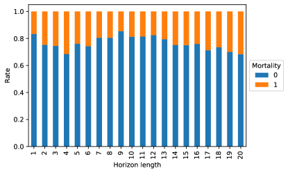
Figure 5: Mortality rates across different horizon lengths.

We consider transferred $Q$-learning across genders. The analytical model for optimal $Q_{t}^{(k)}$ function for each step $t\in[20]$ is modeled by

$$Q_{t}^{(k)}\left(\boldsymbol{x},a\right)\approx\boldsymbol{x}^{\top}\sum_{a^{\prime}=1}^{9}\boldsymbol{\theta}_{t,a^{\prime}}^{(k)}\boldsymbol{1}\left(a=a^{\prime}\right),$$ (23)

where the covariates $\boldsymbol{x}$ contains 44 variables detailed in Table LABEL:tab:variables in the supplements. Even though the total number of trajectories of gender $0$ is large, estimating (23) is still a high-dimensional problem since we allow $\boldsymbol{\theta}_{t,a}^{(k)}$ be different across step $t$, action $a$ and gender subgroup $k=0,1$ and the number of trajectories corresponding to a specific combination of $t$, $a$, and $g$ is small. For example, there are only 19 samples available to estimate $\boldsymbol{\theta}_{t,a}^{(k)}$ for gender $k=1$, step $t=1$, and action $a$ corresponding to the combination $(\textup{IV},\textup{Vaso})=(0,1)$. Table LABEL:tab:least in the supplemental material shows that the least ten samples sizes are all under $30$. We observe that gender $k=1$ (male) has less samples so we consider Transferred $Q$-learning with target task for gender $k=1$ and auxiliary source task from gender $g=0$.

The estimation procedure of Transferred $Q$-learning follows Algorithm 1. We set discount factor as $\gamma=0.98$. We also estimate the $Q$ function by the vanilla $Q$-learning which is the counter part of Algorithm 1 without transfer. The Lasso tuning parameters are chosen according to Theorem 1 and by a linear search for $c_{1}\in$ that maximize the objective function. We calculate the optimal aggregated values of transferred and Vanilla $Q$-learning, denoted by $V^{*,(tl)}$ and $V^{*,(st)}$, respectively. Figure 6 plot the average of the ratio $V^{*,(tl)}/V^{*,(st)}$ and its standard deviation. The mean ratio is above one, indicating that the optimal value of transferred $Q$-learning is larger.

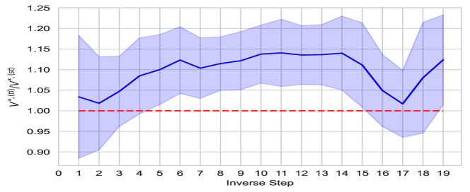
Figure 6: Ratio between optimal aggregated values $V^{*}$ of transferred $Q$-learning ($V^{*,(tl)}$) and those of Vanilla $Q$-learning ($V^{*,(st)}$) applied on the target data. Shaded area covers one standard deviation from the mean. Inverse step is $20-t$ where $1\leq t\leq 20$ is the natural step in a trajectory.

6 Conclusions

In this work, we consider $Q$-learning with knowledge transfer in the form of exploiting more samples from different but similar RL tasks. The similarity between target and source RL tasks is characterized by their corresponding reward functions. We note a salient feature of RL being its multi-stage learning and, accordingly, design a novel re-targeting step to enable vertical information-cascading along multiple steps in a RL task, in addition to the usual horizontal information-gathering in TL for supervised learning. For both offline and online RL tasks, our proposal demonstrates improvements over single-task $Q$-learning theoretically and empirically.

We conclude this paper by pointing out some interesting future directions. As the similarity level is always unknown, it is likely that we include some source tasks which are far away from the target task. To address this concern, one can perform a model selection aggregation step and it guarantees that the aggregated estimator is not much worse than the best performance of the candidate estimators. Aggregation in multi-stage models, especially the online setting, is largely an open problem and requires further investigations.

References

- Ammar et al. (2014) Ammar, H. B., E. Eaton, P. Ruvolo, and M. Taylor (2014). Online multi-task learning for policy gradient methods. In International Conference on Machine Learning, pp. 1206–1214. PMLR.
- Antos et al. (2007) Antos, A., R. Munos, and C. Szepesvari (2007). Fitted Q-iteration in continuous action-space MDPs. In Neural Information Processing Systems.
- Azar et al. (2013) Azar, M. G., R. Munos, and H. J. Kappen (2013). Minimax PAC bounds on the sample complexity of reinforcement learning with a generative model. Machine Learning 91(3), 325–349.
- Azar et al. (2017) Azar, M. G., I. Osband, and R. Munos (2017). Minimax regret bounds for reinforcement learning. In International Conference on Machine Learning, pp. 263–272. PMLR.
- Barreto et al. (2017) Barreto, A., W. Dabney, R. Munos, J. J. Hunt, T. Schaul, D. Silver, and H. P. van Hasselt (2017). Successor features for transfer in reinforcement learning. In NIPS.
- Bastani (2021) Bastani, H. (2021). Predicting with proxies: Transfer learning in high dimension. Management Science 67(5), 2964–2984.
- Boyan (2002) Boyan, J. A. (2002). Technical update: Least-squares temporal difference learning. Machine Learning 49(2), 233–246.
- Chakraborty et al. (2010) Chakraborty, B., S. Murphy, and V. Strecher (2010). Inference for non-regular parameters in optimal dynamic treatment regimes. Statistical Methods in Medical Research 19(3), 317–343.
- Chakraborty and Murphy (2014) Chakraborty, B. and S. A. Murphy (2014). Dynamic treatment regimes. Annual Review of Statistics and its Application 1, 447–464.
- Ernst et al. (2005) Ernst, D., P. Geurts, and L. Wehenkel (2005). Tree-based batch mode reinforcement learning. Journal of Machine Learning Research 6, 503–556.
- Ertefaie et al. (2021) Ertefaie, A., J. R. McKay, D. Oslin, and R. L. Strawderman (2021). Robust q-learning. Journal of the American Statistical Association 116(533), 368–381.
- Ertefaie and Strawderman (2018) Ertefaie, A. and R. L. Strawderman (2018). Constructing dynamic treatment regimes over indefinite time horizons. Biometrika 105(4), 963–977.
- Gupta et al. (2017) Gupta, A., C. Devin, Y. Liu, P. Abbeel, and S. Levine (2017). Learning invariant feature spaces to transfer skills with reinforcement learning. arXiv preprint arXiv:1703.02949.
- Hao et al. (2021) Hao, B., T. Lattimore, C. Szepesvári, and M. Wang (2021). Online sparse reinforcement learning. In International Conference on Artificial Intelligence and Statistics, pp. 316–324. PMLR.
- Jin et al. (2018) Jin, C., Z. Allen-Zhu, S. Bubeck, and M. I. Jordan (2018). Is q-learning provably efficient? In Proceedings of the 32nd International Conference on Neural Information Processing Systems, pp. 4868–4878.
- Jin et al. (2020) Jin, C., Z. Yang, Z. Wang, and M. I. Jordan (2020). Provably efficient reinforcement learning with linear function approximation. In Conference on Learning Theory, pp. 2137–2143.
- Johnson et al. (2016) Johnson, A. E., T. J. Pollard, L. Shen, H. L. Li-wei, M. Feng, M. Ghassemi, B. Moody, P. Szolovits, L. A. Celi, and R. G. Mark (2016). MIMIC-III, a freely accessible critical care database. Scientific data 3, 160035.
- Kallus (2020) Kallus, N. (2020). More efficient policy learning via optimal retargeting. Journal of the American Statistical Association, 1–13.
- Kolm and Ritter (2020) Kolm, P. N. and G. Ritter (2020). Modern perspectives on reinforcement learning in finance. Modern Perspectives on Reinforcement Learning in Finance (September 6, 2019). The Journal of Machine Learning in Finance 1(1).
- Komorowski et al. (2018) Komorowski, M., L. A. Celi, O. Badawi, A. C. Gordon, and A. A. Faisal (2018). The artificial intelligence clinician learns optimal treatment strategies for sepsis in intensive care. Nature medicine 24(11), 1716–1720.
- Lagoudakis and Parr (2003) Lagoudakis, M. G. and R. Parr (2003). Least-squares policy iteration. The Journal of Machine Learning Research 4, 1107–1149.
- Lai and Robbins (1985) Lai, T. L. and H. Robbins (1985). Asymptotically efficient adaptive allocation rules. Advances in Applied Mathematics 6(1), 4–22.
- Langley (2006) Langley, P. (2006). Transfer of knowledge in cognitive systems. In Talk, workshop on Structural Knowledge Transfer for Machine Learning at the Twenty-Third International Conference on Machine Learning.
- Lazaric (2012) Lazaric, A. (2012). Transfer in reinforcement learning: A framework and a survey. In Reinforcement Learning, pp. 143–173. Springer.
- Levine et al. (2020) Levine, S., A. Kumar, G. Tucker, and J. Fu (2020). Offline reinforcement learning: Tutorial, review, and perspectives on open problems. arXiv preprint arXiv:2005.01643.
- Li et al. (2020a) Li, S., T. T. Cai, and H. Li (2020a). Transfer learning for high-dimensional linear regression: Prediction, estimation, and minimax optimality. arXiv:2006.10593.
- Li et al. (2020b) Li, S., T. T. Cai, and H. Li (2020b). Transfer learning in large-scale gaussian graphical models with false discovery rate control. arXiv preprint arXiv:2010.11037.
- Lounici et al. (2009) Lounici, K., M. Pontil, A. Tsybakov, and S. Van De Geer (2009). Taking advantage of sparsity in multi-task learning. In COLT 2009-The 22nd Conference on Learning Theory.
- Luckett et al. (2019) Luckett, D. J., E. B. Laber, A. R. Kahkoska, D. M. Maahs, E. Mayer-Davis, and M. R. Kosorok (2019). Estimating dynamic treatment regimes in mobile health using v-learning. Journal of the American Statistical Association.
- Mehta et al. (2008) Mehta, N., S. Natarajan, P. Tadepalli, and A. Fern (2008). Transfer in variable-reward hierarchical reinforcement learning. Machine Learning 73(3), 289.
- Mousavi et al. (2014) Mousavi, A., B. Nadjar Araabi, and M. Nili Ahmadabadi (2014). Context transfer in reinforcement learning using action-value functions. Computational intelligence and neuroscience 2014.
- Murphy (2005) Murphy, S. (2005). A generalization error for q-learning. Journal of Machine Learning Research: JMLR 6, 1073–1097.
- Murphy (2003) Murphy, S. A. (2003). Optimal dynamic treatment regimes. Journal of the Royal Statistical Society: Series B (Statistical Methodology) 65(2), 331–355.
- Nahum-Shani et al. (2012) Nahum-Shani, I., M. Qian, D. Almirall, W. E. Pelham, B. Gnagy, G. A. Fabiano, J. G. Waxmonsky, J. Yu, and S. A. Murphy (2012). Q-learning: A data analysis method for constructing adaptive interventions. Psychological methods 17(4), 478.
- Parisotto et al. (2016) Parisotto, E., L. J. Ba, and R. Salakhutdinov (2016). Actor-mimic: Deep multitask and transfer reinforcement learning. In ICLR (Poster).
- Prasad et al. (2017) Prasad, N., L. F. Cheng, C. Chivers, M. Draugelis, and B. E. Engelhardt (2017). A reinforcement learning approach to weaning of mechanical ventilation in intensive care units. In 33rd Conference on Uncertainty in Artificial Intelligence, UAI 2017.
- Schulte et al. (2014) Schulte, P. J., A. A. Tsiatis, E. B. Laber, and M. Davidian (2014). Q-and a-learning methods for estimating optimal dynamic treatment regimes. Statistical Science: A Review Journal of the Institute of Mathematical Statistics 29(4), 640.
- Shi et al. (2020) Shi, C., S. Zhang, W. Lu, and R. Song (2020). Statistical inference of the value function for reinforcement learning in infinite horizon settings. arXiv preprint arXiv:2001.04515.
- Sidford et al. (2018) Sidford, A., M. Wang, X. Wu, L. F. Yang, and Y. Ye (2018). Near-optimal time and sample complexities for solving Markov decision processes with a generative model. In Proceedings of the 32nd International Conference on Neural Information Processing Systems, pp. 5192–5202.
- Singla et al. (2021) Singla, A., A. N. Rafferty, G. Radanovic, and N. T. Heffernan (2021). Reinforcement learning for education: Opportunities and challenges. arXiv preprint arXiv:2107.08828.
- Song et al. (2015) Song, R., W. Wang, D. Zeng, and M. R. Kosorok (2015). Penalized -learning for dynamic treatment regimens. Statistica Sinica 25(3), 901.
- Sutton and Barto (2018) Sutton, R. S. and A. G. Barto (2018). Reinforcement Learning: An Introduction. MIT press.
- Taylor and Stone (2007) Taylor, M. E. and P. Stone (2007). Representation transfer for reinforcement learning. In AAAI Fall Symposium: Computational Approaches to Representation Change during Learning and Development, pp. 78–85.
- Taylor and Stone (2009) Taylor, M. E. and P. Stone (2009). Transfer learning for reinforcement learning domains: A survey. Journal of Machine Learning Research 10(7).
- Tripuraneni et al. (2020) Tripuraneni, N., C. Jin, and M. I. Jordan (2020). Provable meta-learning of linear representations. arXiv preprint arXiv:2002.11684.
- Yang and Wang (2019) Yang, L. and M. Wang (2019). Sample-optimal parametric Q-learning using linearly additive features. In International Conference on Machine Learning, pp. 6995–7004. PMLR.