Collisional open quantum dynamics with a generally correlated environment:
Exact solvability in tensor networks

Abstract

Quantum collision models are receiving increasing attention as they describe many nontrivial phenomena in dynamics of open quantum systems. In a general scenario of both fundamental and practical interest, a quantum system repeatedly interacts with individual particles or modes forming a correlated and structured reservoir; however, classical and quantum environment correlations greatly complicate the calculation and interpretation of the system dynamics. Here we propose an exact solution to this problem based on the tensor network formalism. We find a natural Markovian embedding for the system dynamics, where the role of an auxiliary system is played by virtual indices of the network. The constructed embedding is amenable to analytical treatment for a number of timely problems like the system interaction with two-photon wavepackets, structured photonic states, and one-dimensional spin chains. We also derive a time-convolution master equation and relate its memory kernel with the environment correlation function, thus revealing a clear physical picture of memory effects in the dynamics. The results advance tensor-network methods in the fields of quantum optics and quantum transport.

I Introduction

Multipartite quantum systems are notoriously difficult to study. So is the open dynamics of a quantum system interacting with a multipartite or multimode environment. The environment usually consists of enormously many particles or modes, which makes it almost impossible to track the exact dynamics of the system density operator $\varrho_{S}(t)$. The exact treatment of the problem is possible in some exceptional cases only [1, 2, 3, 4, 5, 6, 7], whereas one usually has to resort to some physical approximations, e.g., the weak system-environment coupling with a timescale separation between the bath correlation and the system relaxation [8, 9, 10, 11, 12]. Another approach is based on a past-future independence for environment degrees of freedom interacting with the system [13] — the assumption that is naturally fulfilled in a conventional collision model (also known as the repeated interactions model) with uncorrelated environment particles [14, 15, 16, 17, 18]. The latter approach has received increasing attention in the analysis of quantum nonequilibrium steady states [19, 20, 21], bipartite and multipartite entanglement generation [21, 22, 23], quantum thermodynamical analysis of micromasers [24], quantum thermometry [25], and simulation of open quantum many-body dynamics [26, 27]; see the recent review papers on collision models [28, 29].

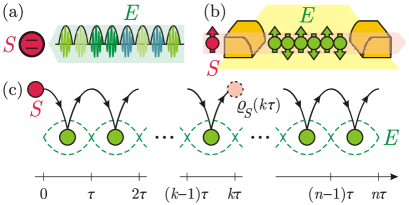
Figure 1: (a) System interaction with an entangled multimode environment state encoded in temporal modes of light. (b) Spin transport through a one-dimensional chain. (c) Quantum collision model with correlated environment.

Collision models naturally emerge in time-bin quantum optics and waveguide quantum electrodynamics, where the radiation field is mapped into a stream of discrete time-bin modes of duration $\tau$ [30, 31, 32, 33, 34, 35, 36, 37, 38, 39] that sequentially interact with the quantum system while the radiation field propagates in space, see Fig. 1(a). However, in contrast to the conventional collision model with a factorized environment, the radiation field represents a correlated and structured environment that is difficult to deal with even in the case of a single-photon wavepacket [40, 41], not to mention entangled multiphoton states generated from the cascade emissions [42, 43] or artificial photonic tensor network states [31, 44, 45, 46, 47, 48, 49]. The latter ones are entangled multimode environment states $\ket{\psi_{E}}$ encoded in temporal modes of light. The greater the number $n$ of time bins the more complicated is the calculation of the system density operator after $k$ collisions,

$$\varrho_{S}(k\tau)={\rm tr}_{1,\ldots,k}\Big{[}U_{Sk}\cdots U_{S1}\varrho_{S}(0)\otimes\varrho_{1\ldots k}\,U_{S1}^{{\dagger}}\cdots U_{Sk}^{{\dagger}}\Big{]},$$ (1)

where $\varrho_{1\ldots k}={\rm tr}_{k+1,\ldots,n}[\ket{\psi_{E}}\bra{\psi_{E}}]$ is the reduced density operator for $k$ environment modes (its dimension growing exponentially with $k$) and $U_{Sk}$ is the evolution operator for the system and the $k$-th mode. Exact and approximate solutions of Eq. (1) are known for some exceptional correlated environments and interactions [50, 51]; however, a general solution to the system dynamics is still missing.

The same computational problem emerges in a collision model for spin transport through a chain of correlated atoms, e.g., a carbon chain [52], where the spin carrier moves ballistically and sequentially interacts with correlated environment particles, see Fig. 1(b). The ground state of a gapped one-dimensional local Hamiltonian for the spin chain has a tensor network structure [53]. A seeming complexity of the tensor network representation, as we show in this paper, is in fact a key to an elegant solution to the computational problem in Eq. (1).

II Tensor network for the environment state

Any pure state of $n$ correlated $d$-dimensional particles adopts the following form of a matrix product state (MPS) [54, 55, 56, 57]:

$$\ket{\psi_{E}}=\sum_{i_{1},i_{2},\ldots,i_{n}=0}^{d-1}B^{[1],i_{1}}B^{[2],i_{2}}\cdots B^{[n],i_{n}}\ket{i_{1}i_{2}\ldots i_{n}},$$ (2)

where index $i_{k}$ corresponds to the distinct physical levels of the $k$-th particle and $B^{[k],i_{k}}$ is a matrix with elements $B^{[k],i_{k}}_{a_{k-1},a_{k}}$ such that the index $a_{k}$ forms a bond between the $k$-th particle and the $(k+1)$-th particle, see Fig. 2(a). The conventional rule for tensor diagrams is that connected lines are summed over. We additionally use arrows to indicate the matrix multiplication order. Indices $a_{0}$ and $a_{n+1}$ are dummy and take the only value, so $B^{[1],i_{1}}$ is a row matrix with elements $B^{[1],i_{1}}_{1,a_{1}}$ and $B^{[n],i_{n}}$ is a column matrix with elements $B^{[n],i_{n}}_{a_{n-1},1}$. $B^{[k]}$ is a rank-3 tensor for $k=2,\ldots,n-1$ and a rank-2 tensor for $k=1,n$. Fig. 2(b) depicts a tensor representation for the environment density operator, where we use complex conjugation (denoted by $\ast$) to construct the bra-vector $\bra{\psi_{E}}$. The partial trace over particles $k+1,\ldots,n$ results in a tensor contraction shown in Fig. 2(c). This contraction becomes much simpler if we rewrite the MPS in the right-canonical form (which is always possible [56, 57]), where

$$\sum_{i_{k}=1}^{d}B^{[k],i_{k}}(B^{[k],i_{k}})^{{\dagger}}=I_{k-1},$$ (3)

with $I_{k-1}$ being the $|\{a_{k-1}\}|\times|\{a_{k-1}\}|$ identity matrix. Then $\varrho_{1\ldots k}$ entirely depends on tensors $B^{[1]},\ldots,B^{[k]}$, with the irrelevant (future) particles $k+1,\ldots,n$ being replaced by a single connecting line, see Fig. 2(d). Fig. 2(d) contains an extra tensor $\chi_{0}$, which is a trivial $1\times 1$ identity matrix in the case of a pure environment. If the environment density operator is a mixture $\varrho_{E}=\sum_{q}p_{q}\ket{\psi_{E}^{q}}\bra{\psi_{E}^{q}}$, where each MPS $\ket{\psi_{E}^{q}}$ adopts the right-canonical form with matrices $B^{[q,k],i_{k}}$, then $\chi_{0}={\rm diag}(p_{1},p_{2},\ldots)$ and $B^{[k],i_{k}}=\bigoplus_{q}B^{[q,k],i_{k}}$. Therefore, the tensor diagram for in Fig. 2(d) is equally applicable to both pure and mixed environment states. One could alternatively use the formalism of matrix product density operators [58, 59] to represent the mixed environment; however, this would not change the main idea and would merely result in a slight modification of the Kraus operators presented in Section III.1 (see the review [60] inspired by this paper).

The presented formalism is also applicable to the case when the environment represents an infinite chain of particles in both directions, e.g., the famous Affleck-Kennedy-Lieb-Tasaki (AKLT) antiferromagnetic spin chain [61]. The first collision happens with some intermediate particle (the past particles are assumed to be unaccessible). The partial trace over the past particles results in the positive semidefinite matrix $\chi_{0}$ with unit trace. In all the scenarios, $\chi_{0}$ is a density matrix for bond degrees for freedom. To deal with the bond degrees of freedom, we formally introduce an auxiliary Hilbert space ${\cal H}_{\text{bond}\#k}$ spanning orthonormal vectors $\{\ket{a_{k}}\}$ as is shown in Fig. 2(d). The matrix $B^{[k],i_{k}}$ defines a mapping from ${\cal H}_{\text{bond}\#k}$ to ${\cal H}_{\text{bond}\#(k-1)}$ (from right to left in Fig. 2), whereas the transposed matrix $(B^{[k],i_{k}})^{\top}$ defines a mapping from ${\cal H}_{\text{bond}\#(k-1)}$ to ${\cal H}_{\text{bond}\#k}$ (from left to right).

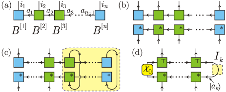
Figure 2: Tensor diagrams for matrix product state $\ket{\psi_{E}}$ (a), density operator $\ket{\psi_{E}}\bra{\psi_{E}}$ (b), reduced density operator (c) and its equivalent if environment has the right-canonical form (d). The bond Hilbert space ${\cal H}_{\text{bond}\#k}=\text{Span}(\{\ket{a_{k}}\})$. Outcoming and incoming arrows stand for ket- and bra-components, respectively.

The maximum bond dimension $\max_{k}|\{a_{k}\}|$ (the MPS rank) for a general state scales exponentially with the number of particles; however, if the state is slightly entangled in terms of the entanglement entropy [with potentially long correlations as in the Greenberger-Horne-Zeilinger (GHZ) state], then such a state can be efficiently described in the right-canonical form with a rather small bond dimension [62]. For instance, the MPS rank equals $2$ for the GHZ state of $n$ qubits, the AKLT state of $n$ qutrits, the photonic cluster state [46, 47], and an arbitrary single-photon wavepacket $\ket{\psi_{E}}=c_{1}\ket{100\ldots 00}+c_{2}\ket{010\ldots 00}+\ldots+c_{n}\ket{000\ldots 01}$. We consider some of these states and a two-photon state from the cascade emission with the MPS rank $3$ as examples in subsequent sections.

III System dynamics

III.1 Markovian embedding

Were the environment uncorrelated, the system evolution would be described by sequential applications of quantum channels $\widetilde{\Phi}_{k}$ defined through $\widetilde{\Phi}_{k}[\varrho_{S}]={\rm tr}_{k}[U_{Sk}\varrho_{S}\otimes\varrho_{k}U_{Sk}^{{\dagger}}]$, where $\varrho_{k}$ is a density operator for the $k$-th environment particle. As this is not the case, we have to draw a full tensor diagram for collisions in Fig. 3(a). Upper $\cap$-lines correspond to the trace over environment particles, which the system has already interacted with. Looking at the diagram from left to right, we observe the evolution of a rank-4 tensor $R(k\tau)$ that is a composite system-bond density operator on the Hilbert space ${\cal H}_{S}\otimes{\cal H}_{\text{bond}\#k}$ with $R(0)=\varrho_{S}(0)\otimes\chi_{0}$. Due to the right-normalization condition (3), the partial trace for $R(k\tau)$ over bond degrees of freedom effectively produces the reduced environment state $\varrho_{1\ldots k}$ at the bottom of the diagram and Eq. (1) yields the system density operator,

$$\varrho_{S}(k\tau)={\rm tr}_{\text{bond}\#k}[R(k\tau)].$$ (4)

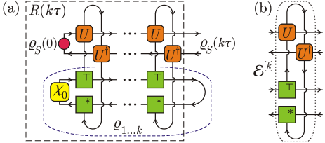
Figure 3: (a) Tensor network diagram for the system density operator $\varrho_{S}(k\tau)$ and the system-bond density operator $R(k\tau)$ after $k$ collisions. (b) Completely positive and trace preserving map ${\cal E}^{[k]}$.

These are the bond indices through which the information about the previous collisions propagates in time and affects the system evolution long time after the collisions actually happened. Time evolution of the tensor $R$ is governed by unitary operators $U_{Sk}$ as well as by tensors $(B^{[k],i_{k}})^{\top}$ that start playing a role of evolution operators for the bond degrees of freedom. The system-bond dynamics is given by a recurrent relation

$$R(k\tau)={\cal E}^{[k]}\left[R\big{(}(k-1)\tau\big{)}\right],$$ (5)

where a propagator map ${\cal E}^{[k]}$ is depicted in Fig. 3(b). This map is completely positive and trace preserving due to the unitarity of $U_{Sk}$ and the right-normalization condition (3). A diagonal sum representation ${\cal E}^{[k]}[\bullet]=\sum_{j_{k}}A_{j_{k}}\bullet A_{j_{k}}^{{\dagger}}$ has the Kraus operators

$$A_{j_{k}}=\sum_{i_{k}}\bra{j_{k}}U_{Sk}\ket{i_{k}}\otimes(B^{[k],i_{k}})^{\top}$$ (6)

depicted in Fig. 4(a). Eqs. (4) and (5) manifest the Markovian embedding for the system dynamics. Such embeddings are of great use in description of open quantum systems [63, 64, 65, 66, 67]. Previous studies on Markovian embeddings for collision models assumed no initial correlations in the environment [68, 69]. Our construction is valid for a generally correlated MPS environment, with the MPS rank being a dimension of an “effective reservoir” in the embedding. A different but similar tensor network consideration of an approximate Markovian embedding for a rather general open system dynamics is reported in Ref. [70].

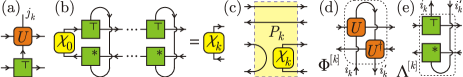
Figure 4: Elementary tensor diagrams.

III.2 Case study: Interaction with a two-photon wavepacket

Consider a two-level system in the ground state $\ket{g}$. The system is exposed to a two-photon wavepacket, e.g., generated from the cascade emissions [42, 43], with the time-bin representation $\ket{\psi_{E}}\propto\sum_{l,m}e^{-l\tau/T_{1}}e^{-m\tau/T_{2}}\ket{0\ldots 01_{l}0\ldots 01_{l+m}0\ldots}$. Each photon has an exponentially decaying temporal profile; however, the second photon can only be emitted after the first one. Such a wavepacket is a right-canonical MPS of rank $3$, where $\chi_{0}={\rm diag}(1,0,0)$, $B^{[k],0}={\rm diag}(e^{-\tau/T_{1}},e^{-\tau/T_{2}},1)$, and $B^{[k],1}$ has two non-zero elements $B^{[k],1}_{a,a+1}=\sqrt{1-e^{-2\tau/T_{a}}}$, $a=1,2$ for all $k$ [71]. The energy levels of the system interact with each time-bin mode via the excitation-preserving exchange $U=\exp[g\tau(\ket{e}\bra{g}\otimes a^{{\dagger}}-\ket{g}\bra{e}\otimes a)]$, where $g$ has the physical dimension of frequency, $a$ and $a^{{\dagger}}$ are the photon annihilation and creation operators, respectively. We treat $U$ as a $3\times 3$ matrix because only $j_{k}=0,1,2$ photons in each mode are possible. The developed Markovian embedding theory enables us to readily calculate the excited state population $p(t)=\bra{e}\varrho_{S}(t)\ket{e}$, see Fig. 5(a). The population dynamics significantly differs from that for a factorized radiation field $\bigotimes_{i}\varrho_{i}$, which illustrates the strong effect of environment correlations on the system dynamics.

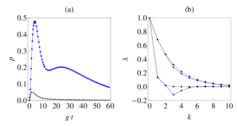
Figure 5: (a) Excited level population vs dimensionless time for a system interacting with a correlated two-photon wavepacket (upper solid line). Disregard of correlations results in the lower dashed line. Parameters $g\tau=0.3$, $gT_{1}=2.3$, $gT_{2}=59.9$. (b) Qubit coherence function vs number of system collisions with a linear cluster state. Exact solution (blue solid lines) and uncorrelated environment approximation (black dashed lines) for parameters $g\tau=0.3$ (upper two lines) and $g\tau=0.6$ (lower two lines).

III.3 Case study: Interaction with a photonic cluster state

The environment state $\ket{\psi_{E}}$ is given by matrices $\chi_{0}={\rm diag}(1,0)$, $B^{[k],0}=\frac{1}{\sqrt{2}}\left(\begin{array}[]{cc}1&0\\ 1&0\\ \end{array}\right)$, and $B^{[k],1}=\frac{1}{\sqrt{2}}\left(\begin{array}[]{cc}0&1\\ 0&-1\\ \end{array}\right)$ for all $k$, which encode, e.g., photon-number entanglement between modes [38]. Let a single system-mode interaction be $U=\exp[g\tau(\ket{e}\bra{g}+\ket{g}\bra{e})\otimes(a-a^{{\dagger}})]$. Eqs. (4)–(6), where $j_{k}$ is now unlimited, result in a dephasing system dynamics with the coherence basis states $(\ket{g}\pm\ket{e})/\sqrt{2}$ and the decoherence function $\lambda$ shown in Fig. 5(b). The figure also depicts the coherence function if the environment correlations are disregarded. Moreover, the first two collisions result in the same dynamics for both correlated and uncorrelated environments. A question arises: Why do correlated and uncorrelated environments result in very different dynamics in Fig. 5(a) and very close dynamics in Fig. 5(b)? To anticipate the detailed analysis, which we provide in what follows, the reason for that behavior is the two-point environment correlation function, which significantly differs from zero for the two-photon wavepacket and vanishes for the cluster state. The small deviation in Fig. 5(b) is due to higher-order environment correlations.

IV Master equation

IV.1 Memory kernel and two-point correlations

Though the Markovian embedding technique provides a universal recipe for the system dynamics, the physics of dynamical memory effects gets clearer in the time-convolution master equation,

$$\frac{\varrho_{S}\big{(}(k+1)\tau\big{)}-\varrho_{S}(k\tau)}{\tau}=\sum_{m=0}^{k}{\cal K}_{km}[\varrho_{S}\big{(}(k-m)\tau\big{)}],$$ (7)

where the memory kernel map ${\cal K}_{km}$ relates the density matrix increment with the past density operators. A time-local term ${\cal K}_{k0}$ gives the density operator increment caused by the latest collision (among those that have already happened), whereas ${\cal K}_{km}$ for $m\geq 1$ describes a nontrivial effect of $m$ preceding collisions on the system evolution. To derive the memory kernel we use the standard projection operator techniques [72] and adapt them to our collision model. The main modification is in the time-dependent nature of projection $P_{k}$ applied at time $k\tau$ to the system-bond density operator. We define $P_{k}[R]={\rm tr}_{\text{bond}\#k}[R]\otimes\chi_{k}$, where $\chi_{k}$ is a bond density operator induced by a “free evolution” for the bond degrees of freedom, i.e., $\chi_{k}=\sum_{i_{k}}(B^{[k],i_{k}})^{\top}\chi_{k-1}(B^{[k],i_{k}})^{\ast}$, see Figs. 4(b,c). The projection $P_{k}$ breaks the past-future correlations in the environment and yields $P_{k}[R(k\tau)]=\varrho_{S}(k\tau)\otimes\chi_{k}$. Inserting the identity transformation ${\rm Id}_{S+\text{bond}\#k}=P_{k}+Q_{k}$, where $Q_{k}$ is a complementary projection, in Eq. (5), we solve a recurrent equation on $Q_{k}[R(k\tau)]$ with the initial condition $Q_{0}[R(0)]=0$ and get an explicit solution for $P_{k+1}[R\big{(}(k+1)\tau\big{)}]$, which yields the following kernel components: the local term ${\cal K}_{k0}[\varrho_{S}]=\frac{1}{\tau}(\widetilde{\Phi}_{k+1}[\varrho_{S}]-\varrho_{S})$ and the nonlocal term ${\cal K}_{km}[\varrho_{S}]=\frac{1}{\tau}{\rm tr}_{\text{bond}\#(k+1)}\circ{\cal E}^{[k+1]}\circ Q_{k}\circ{\cal E}^{[k]}\circ\ldots\circ Q_{k-m+1}\circ{\cal E}^{[k-m+1]}[\varrho_{S}\otimes\chi_{k-m}]$. The local term is the only contribution to the memory kernel in the absence of environment correlations.

To understand the nonlocal term, we decompose the embedding map ${\cal E}^{[k]}=\sum_{i_{k},i^{\prime}_{k}}\Phi^{[k]}_{i_{k}i^{\prime}_{k}}\otimes\Lambda^{[k]}_{i_{k}i^{\prime}_{k}}$ into two parts, where only $\Phi^{[k]}_{i_{k}i^{\prime}_{k}}$ depends on the interaction nature, see Figs. 4(d,e). Then we find a series expansion for $\Phi^{[k]}_{i_{k}i^{\prime}_{k}}$ with respect to the interaction strength $g\tau$ between the system and an individual environment particle. Here we assume that the system-particle interaction Hamiltonian during the $k$-th collision is $g\hbar H_{k}$, where $\hbar$ is the reduced Planck constant and $H_{k}$ is a dimensionless Hermitian operator with the operator norm $\|H_{k}\|\leq 1$. A straightforward contraction of the tensor diagram for ${\cal K}_{km}$ yields the following largest contribution to the memory kernel that comes from the second-order perturbation:

$${\cal K}_{km}^{(2)}[\varrho_{S}]=-g^{2}\tau\left.{\cal C}_{ll^{\prime}}\left(\Big{[}H_{l},\big{[}H_{l^{\prime}},\varrho_{S}\big{]}\Big{]}\right)\right|_{l=k+1,l^{\prime}=k-m+1},$$ (8)

where $[\cdot,\cdot]$ denotes the commutator and ${\cal C}_{ll^{\prime}}(\bullet)={\rm tr}_{l,l^{\prime}}[\bullet(\varrho_{l,l^{\prime}}-\varrho_{l}\otimes\varrho_{l^{\prime}})]$ is a two-point operator-valued correlation function. For instance, ${\cal C}_{ll^{\prime}}(H_{l}\varrho_{S}H_{l^{\prime}})=\langle H_{l}\varrho_{S}H_{l^{\prime}}\rangle_{E}-\langle H_{l}\rangle_{E}\varrho_{S}\langle H_{l^{\prime}}\rangle_{E}$. Eq. (8) provides an important physical link between the environment correlation function and the memory kernel.

IV.2 Stroboscopic limit

If $\tau\ll 1/g$, then $\frac{1}{2\tau}[\varrho_{S}\big{(}(k+1)\tau\big{)}-\varrho_{S}\big{(}(k-1)\tau\big{)}]=\frac{d\varrho_{S}(t)}{dt}+O(g^{3}\tau^{2})$, where $t=k\tau$ is a continuous time. If additionally the environment correlation length $l_{\rm corr}$ is finite, then we can neglect the contribution of $m$-point correlations ($m\geq 3$) in ${\cal K}_{km}$ and get the celebrated Nakajima-Zwanzig equation [73, 74] $\frac{d\varrho_{S}(t)}{dt}=\int_{0}^{t}K(t^{\prime})[\varrho_{S}(t-t^{\prime})]dt^{\prime}$ for a homogeneous collision model, where $U_{Sk}$, $B^{[k]}$, and $\chi_{k}$ do not depend on $k$. The kernel $K(t^{\prime})[\varrho_{S}]=\delta(t^{\prime})L_{\rm local}[\varrho_{S}]+\frac{1}{2}g^{2}\tau\sum_{m=1}^{\infty}\delta(t^{\prime}-m\tau)K_{m}[\varrho_{S}]+O(g^{3}\tau^{2})$, where $\delta$ is the Dirac delta function, $L=\frac{1}{2\tau}(\widetilde{\Phi}_{12}-{\rm Id}_{S})$ originates from two sequential collisions, and $K_{m}[\varrho_{S}]=\big{[}\langle H\rangle_{E},[\langle H\rangle_{E},\varrho_{S}]\big{]}-\left\langle\big{[}H_{m+1},[H_{1},\varrho_{S}\otimes I_{E}]\big{]}\right\rangle_{E}$ describes the exponentially decaying correlations in an MPS [54, 55, 56, 57], so $K_{m}[\varrho_{S}]=(\pm 1)^{m}e^{-m/l_{\rm corr}}L_{\rm nonlocal}[\varrho_{S}]$, where $\pm$ is a sign of the second largest eigenvalue of the transfer matrix. The kernel $K(t^{\prime})$ is the inverse Laplace transform [75, 76] of $(\pm e^{s\tau+l_{\rm corr}^{-1}}-1)^{-1}L_{\rm nonlocal}$. In the stroboscopic limit $g\tau\rightarrow 0$, $g^{2}\tau={\rm const}$, which is discussed in Refs. [77, 78, 79], we get the exact equation $\frac{d\varrho_{S}(t)}{dt}=L[\varrho_{S}(t)]$ of the Gorini-Kossakowski-Sudarshan-Lindblad form [80, 81] with $L=L_{\rm local}+\frac{1}{2}g^{2}\tau(\pm e^{l_{\rm corr}^{-1}}-1)^{-1}L_{\rm nonlocal}$. Importantly, the relaxation rate in $L$ may significantly differ from that in $L_{\rm local}$. Higher order stroboscopic limits are discussed in more detail in the review [60] inspired by this paper.

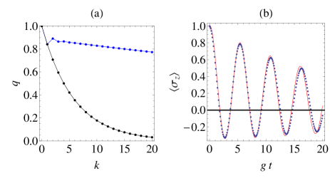
Figure 6: (a) Qubit depolarization parameter vs number of Heisenberg-interaction collisions with the AKLT spin chain: exact solution (upper line) and uncorrelated environment assumption (lower line). (b) Qubit observable vs dimensionless time in an exemplary collisional dynamics with the AKLT environment: exact (dots) and stroboscopic limit (solid line).

IV.3 Case study: Interaction with AKLT infinite spin chain

The AKLT state of spin-1 particles is a right-canonical MPS of rank $2$ with matrices $B^{[k],0}={\rm diag}(-1/\sqrt{3},1/\sqrt{3})$ and $B^{[k],\pm 1}$ that have the only nonzero element $B^{[k],1}_{12}=-B^{[k],-1}_{21}=\sqrt{2/3}$. At time $t=0$ a qubit system collides with one of the chain spins, then collides with its right neighbor and so on. In this scenario, $\chi_{0}=\frac{1}{2}I$. Consider the Heisenberg-type qubit-spin interaction $U=\exp[-\frac{g\hbar}{2}(\sigma_{x}\otimes J_{x}+\sigma_{y}\otimes J_{y}+\sigma_{z}\otimes J_{z})]$, where $(\sigma_{x},\sigma_{y},\sigma_{z})$ is the set of Pauli matrices and $J_{\alpha}$ is an operator for the spin projection (in units of $\hbar$) on the $\alpha$ direction. The AKLT state has exponentially decaying two-point correlations because $\varrho_{1m}=\frac{1}{3}I\otimes\frac{1}{3}I+\left(-\frac{1}{3}\right)^{m}\left(J_{x}\otimes J_{x}+J_{y}\otimes J_{y}+J_{z}\otimes J_{z}\right)$; however, these correlations are strong enough to significantly deviate the qubit dynamics from that for the uncorrelated environment. The disregard of environment correlations yields the qubit dynamics $\varrho_{S}(t)=q(t)\varrho_{S}(0)+[1-q(t)]\frac{1}{2}I$, where the depolarization function $q_{\rm Markov}(k\tau)=[\frac{1}{27}\left(11+16\cos\frac{3}{2}g\tau\right)]^{k}$ has the asymptotic behavior $q_{\rm Markov}(t)\approx\exp(-\frac{2}{3}g^{2}\tau t)$ if $g\tau\ll 1$. However, the exact qubit dynamics is given by $q(k\tau)=\left(\frac{1}{2}+\frac{x}{z}\right)\left(\frac{y+z}{27}\right)^{k}+\left(\frac{1}{2}-\frac{x}{z}\right)\left(\frac{y-z}{27}\right)^{k}$, where $x=2+7\cos\frac{3g\tau}{2}$, $y=7+2\cos\frac{3}{2}g\tau$, $z=2\sqrt{y^{2}+27\sin^{2}\frac{3}{2}g\tau}$. Hence, $q(t)\approx(1-\frac{1}{2}g^{2}\tau^{2})\exp(-\frac{1}{8}g^{4}\tau^{3}t)$ if $g\tau\ll 1$, see Fig. 6(a). The exponent power vanishes in the stroboscopic limit, so does $L$. To demonstrate efficacy of the stroboscopic-limit equation $\frac{d\varrho_{S}(t)}{dt}=L[\varrho_{S}(t)]$ with nonvanishing decoherence rate, we consider a controlled unitary interaction $U=e^{-ig\tau\sigma_{x}}\otimes\ket{+1}\bra{+1}+e^{-ig\tau\sigma_{y}}\otimes\ket{0}\bra{0}+e^{-ig\tau\sigma_{z}}\otimes\ket{-1}\bra{-1}$ with $g\tau=0.1$ and show a good agreement between the exact and approximate dynamics in Fig. 6(b). These examples illustrate that the two-point environment correlations correctly describe the system dynamics under the stroboscopic assumption $g\tau\ll 1$ if $l_{\rm corr}$ is finite. If $l_{\rm corr}=\infty$ (e.g., for the GHZ state), then multitime correlation functions are to be taken into consideration too.

V Conclusions

We have presented two approaches to the collisional open quantum dynamics with a generally correlated environment: the Markovian embedding in Eqs. (4)–(5) and the time-convolution master equation (7) with its continuous limit. The former approach readily provides a solution to a number of timely problems like the system interaction with two-photon wavepackets, structured photonic states, and one-dimensional spin chains. The latter approach reveals the physics of memory effects and its relation to the environment correlation functions. Here we have demonstrated the advantages of tensor networks in general collisional dynamics, thus extending the range of successful tensor-network applications in many-body dynamics [82, 83, 84], operational meaning of non-Markovianity [85, 86, 87], and spin-boson models [88, 89, 90].

References

- [1] A. O. Caldeira and A. Leggett, Phys. A (Amsterdam, Neth.) 121, 587 (1983).
- [2] B. L. Hu, J. P. Paz, and Y. Zhang, Quantum Brownian motion in a general environment: exact master equation with nonlocal dissipation and colored noise, Phys. Rev. D 45, 2843 (1992).
- [3] G. M. Palma, K.-A. Suominen, and A. K. Ekert, Quantum computers and dissipation, Proc. R. Soc. A 452, 567 (1996).
- [4] B. Vacchini and H.-P. Breuer, Exact master equations for the non-Markovian decay of a qubit, Phys. Rev. A 81, 042103 (2010).
- [5] L. Ferialdi, Exact closed master equation for Gaussian non-Markovian dynamics, Phys. Rev. Lett. 116, 120402 (2016).
- [6] Y.-L. L. Fang, F. Ciccarello, and H. U. Baranger, Non-Markovian dynamics of a qubit due to single-photon scattering in a waveguide, New J. Phys. 20, 043035 (2018).
- [7] D. Burgarth, P. Facchi, M. Ligabò, and D. Lonigro, Hidden non-Markovianity in open quantum systems, Phys. Rev. A 103, 012203 (2021).
- [8] E. B. Davies, Markovian master equations, Commun. Math. Phys. 39, 91 (1974).
- [9] G. Schaller and T. Brandes, Preservation of positivity by dynamical coarse graining, Phys. Rev. A 78, 022106 (2008).
- [10] F. Benatti, R. Floreanini, and U. Marzolino, Entangling two unequal atoms through a common bath, Phys. Rev. A 81, 012105 (2010).
- [11] Á. Rivas, Refined weak-coupling limit: Coherence, entanglement, and non-Markovianity, Phys. Rev. A 95, 042104 (2017).
- [12] A. Trushechkin, Unified Gorini-Kossakowski-Lindblad-Sudarshan quantum master equation beyond the secular approximation, Phys. Rev. A 103, 062226 (2021).
- [13] L. Li, M. J. W. Hall, and H. M. Wiseman, Concepts of quantum non-Markovianity: A hierarchy, Phys. Rep. 759, 1 (2018).
- [14] J. Rau, Relaxation phenomena in spin and harmonic oscillator systems, Phys. Rev. 129, 1880 (1963).
- [15] V. Scarani, M. Ziman, P. Štelmachovič, N. Gisin, and V. Bužek, Thermalizing quantum machines: Dissipation and entanglement, Phys. Rev. Lett. 88, 097905 (2002).
- [16] S. Attal and Y. Pautrat, From repeated to continuous quantum interactions, Ann. Henri Poincaré 7, 59 (2006).
- [17] C. Pellegrini and F. Petruccione, Non-Markovian quantum repeated interactions and measurements, J. Phys. A: Math. Theor. 42, 425304 (2009).
- [18] D. Grimmer, D. Layden, R. B. Mann, and E. Martın-Martınez, Open dynamics under rapid repeated interaction, Phys. Rev. A 94, 032126 (2016).
- [19] D. Karevski and T. Platini, Quantum nonequilibrium steady states induced by repeated interactions, Phys. Rev. Lett. 102, 207207 (2009).
- [20] R. Román-Ancheyta, M. Kolář, G. Guarnieri, and R. Filip, Enhanced steady-state coherence via repeated system-bath interactions, Phys. Rev. A 104, 062209 (2021).
- [21] D. Heineken, K. Beyer, K. Luoma, and W. T. Strunz, Quantum-memory-enhanced dissipative entanglement creation in nonequilibrium steady states, Phys. Rev. A 104, 052426 (2021).
- [22] S. Daryanoosh, B. Q. Baragiola, T. Guff, and A. Gilchrist, Quantum master equations for entangled qubit environments, Phys. Rev. A 98, 062104 (2018).
- [23] B. Çakmak, S. Campbell, B. Vacchini, Ö. E. Müstecaplıoğlu, and M. Paternostro, Robust multipartite entanglement generation via a collision model, Phys. Rev. A 99, 012319 (2019).
- [24] P. Strasberg, G. Schaller, T. Brandes, and M. Esposito, Quantum and information thermodynamics: A unifying framework based on repeated interactions, Phys. Rev. X 7, 021003 (2017).
- [25] S. Seah, S. Nimmrichter, D. Grimmer, J. P. Santos, V. Scarani, and G. T. Landi, Collisional quantum thermometry, Phys. Rev. Lett. 123, 180602 (2019).
- [26] A. Purkayastha, G. Guarnieri, S. Campbell, J. Prior, and J. Goold, Periodically refreshed baths to simulate open quantum many-body dynamics, Phys. Rev. B 104, 045417 (2021).
- [27] M. Cattaneo, G. De Chiara, S. Maniscalco, R. Zambrini, and G. L. Giorgi, Collision models can efficiently simulate any multipartite Markovian quantum dynamics, Phys. Rev. Lett. 126, 130403 (2021).
- [28] F. Ciccarello, S. Lorenzo, V. Giovannetti, G. M. Palma, Quantum collision models: open system dynamics from repeated interactions, arXiv:2106.11974 [quant-ph].
- [29] S. Campbell, B. Vacchini, Collision models in open system dynamics: A versatile tool for deeper insights? EPL 133, 60001 (2021).
- [30] H. Pichler and P. Zoller, Photonic circuits with time delays and quantum feedback, Phys. Rev. Lett. 116, 093601 (2016).
- [31] P.-O. Guimond, M. Pletyukhov, H. Pichler, and P. Zoller, Delayed coherent quantum feedback from a scattering theory and a matrix product state perspective, Quantum Sci. Technol. 2, 044012 (2017).
- [32] F. Ciccarello, Collision models in quantum optics, Quantum Measurements and Quantum Metrology 4, 53 (2017).
- [33] J. A. Gross, C. M. Caves, G. J. Milburn, and J. Combes, Qubit models of weak continuous measurements: markovian conditional and open-system dynamics, Quantum Sci. Technol. 3, 024005 (2018).
- [34] K. A. Fischer, R. Trivedi, V. Ramasesh, I. Siddiqi, and J. Vučković, Scattering into one-dimensional waveguides from a coherently-driven quantum-optical system, Quantum 2, 69 (2018).
- [35] D. Cilluffo, A. Carollo, S. Lorenzo, J. A. Gross, G. M. Palma, and F. Ciccarello, Collisional picture of quantum optics with giant emitters, Phys. Rev. Research 2, 043070 (2020).
- [36] A. Carmele, N. Nemet, V. Canela, and S. Parkins, Pronounced non-Markovian features in multiply excited, multiple emitter waveguide QED: Retardation induced anomalous population trapping, Phys. Rev. Research 2, 013238 (2020).
- [37] V. S. Ferreira, J. Banker, A. Sipahigil, M. H. Matheny, A. J. Keller, E. Kim, M. Mirhosseini, and O. Painter, Collapse and revival of an artificial atom coupled to a structured photonic reservoir, Phys. Rev. X 11, 041043 (2021).
- [38] S. C. Wein, J. C. Loredo, M. Maffei, P. Hilaire, A. Harouri, N. Somaschi, A. Lemaître, I. Sagnes, L. Lanco, O. Krebs, A. Auffèves, C. Simon, P. Senellart, and C. Antón-Solanas, Photon-number entanglement generated by sequential excitation of a two-level atom, arXiv:2106.02049 [quant-ph].
- [39] M. Maffei, P. A. Camati, and A. Auffèves, Closed-system solution of the 1D atom from collision model, Entropy 24, 151 (2022).
- [40] A. M. Dąbrowska, From a posteriori to a priori solutions for a two-level system interacting with a single-photon wavepacket, J. Opt. Soc. Am. B 37, 1240 (2020).
- [41] A. Dąbrowska, D. Chruściński, S. Chakraborty, and G. Sarbicki, Eternally non-Markovian dynamics of a qubit interacting with a single-photon wavepacket, New J. Phys. 23, 123019 (2021).
- [42] H. H. Jen, Cascaded cold atomic ensembles in a diamond configuration as a spectrally entangled multiphoton source, Phys. Rev. A 95, 043840 (2017).
- [43] A. Cerè, B. Srivathsan, G. Kaur Gulati, B. Chng, and C. Kurtsiefer, Characterization of a photon-pair source based on a cold atomic ensemble using a cascade-level scheme, Phys. Rev. A 98, 023835 (2018).
- [44] I. Dhand, M. Engelkemeier, L. Sansoni, S. Barkhofen, C. Silberhorn, and M. B. Plenio, Proposal for quantum simulation via all-optically-generated tensor network states, Phys. Rev. Lett. 120, 130501 (2018).
- [45] M. Lubasch, A. A. Valido, J. J. Renema, W. S. Kolthammer, D. Jaksch, M. S. Kim, I. Walmsley, and R. Garcıa-Patrón, Tensor network states in time-bin quantum optics, Phys. Rev. A 97, 062304 (2018).
- [46] D. Istrati, Y. Pilnyak, J. C. Loredo, C. Antón, N. Somaschi, P. Hilaire, H. Ollivier, M. Esmann, L. Cohen, L. Vidro, C. Millet, A. Lemaître, I. Sagnes, A. Harouri, L. Lanco, P. Senellart, and H. S. Eisenberg, Sequential generation of linear cluster states from a single photon emitter, Nat. Commun. 11, 5501 (2020).
- [47] J.-C. Besse, K. Reuer, M. C. Collodo, A. Wulff, L. Wernli, A. Copetudo, D. Malz, P. Magnard, A. Akin, M. Gabureac, G. J. Norris, J. I. Cirac, A. Wallraff, and C. Eichler, Realizing a deterministic source of multipartite-entangled photonic qubits, Nat. Commun. 11, 4877 (2020).
- [48] K. Tiurev, M. H. Appel, P. L. Mirambell, M. B. Lauritzen, A. Tiranov, P. Lodahl, and A. S. Sørensen, High-fidelity multi-photon-entangled cluster state with solid-state quantum emitters in photonic nanostructures, arXiv:2007.09295 [quant-ph].
- [49] Z.-Y. Wei, D. Malz, A. González-Tudela, and J. I. Cirac, Generation of photonic matrix product states with Rydberg atomic arrays, Phys. Rev. Research 3, 023021 (2021).
- [50] T. Rybár, S. N. Filippov, M. Ziman, and V. Bužek, Simulation of indivisible qubit channels in collision models, J. Phys. B: At. Mol. Opt. Phys. 45, 154006 (2012).
- [51] S. N. Filippov, J. Piilo, S. Maniscalco, and M. Ziman, Divisibility of quantum dynamical maps and collision models, Phys. Rev. A 96, 032111 (2017).
- [52] Z. Zanolli, G. Onida, and J.-C. Charlier. Quantum spin transport in carbon chains. ACS Nano 4, 5174 (2010).
- [53] A. M. Dalzell and F. G. S. L. Brandão, Locally accurate MPS approximations for ground states of one-dimensional gapped local Hamiltonians, Quantum 3, 187 (2019).
- [54] D. Pérez-García, F. Verstraete, M. M. Wolf, and J. I. Cirac, Matrix product state representations, Quantum Information and Computation 7, 401 (2007).
- [55] F. Verstraete, V. Murg, and J. I. Cirac, Matrix product states, projected entangled pair states, and variational renormalization group methods for quantum spin systems, Advances in Physics 57, 143 (2008).
- [56] U. Schollwöck, The density-matrix renormalization group in the age of matrix product states, Annals of Physics 326, 96 (2011).
- [57] J. I. Cirac, D. Pérez-García, N. Schuch, and F. Verstraete, Matrix product states and projected entangled pair states: Concepts, symmetries, theorems, Rev. Mod. Phys. 93, 045003 (2021).
- [58] F. Verstraete, J. J. García-Ripoll, and J. I. Cirac, Matrix product density operators: Simulation of finite-temperature and dissipative systems, Phys. Rev. Lett. 93, 207204 (2004).
- [59] M. Zwolak and G. Vidal, Mixed-state dynamics in one-dimensional quantum lattice systems: A time-dependent superoperator renormalization algorithm, Phys. Rev. Lett. 93, 207205 (2004).
- [60] S. N. Filippov. Multipartite correlations in quantum collision models. Entropy 24, 508 (2022).
- [61] I. Affleck, T. Kennedy, E. H. Lieb, and H. Tasaki, Rigorous results on valence-bond ground states in antiferromagnets, Phys. Rev. Lett. 59, 799 (1987).
- [62] G. Vidal, Efficient classical simulation of slightly entangled quantum computations, Phys. Rev. Lett. 91, 147902 (2003).
- [63] J. Iles-Smith, A. G. Dijkstra, N. Lambert, and A. Nazir, Energy transfer in structured and unstructured environments: Master equations beyond the Born-Markov approximations, J. Chem. Phys. 144, 044110 (2016).
- [64] D. Tamascelli, A. Smirne, S. F. Huelga, and M. B. Plenio, Nonperturbative Ttreatment of non-Markovian dynamics of open quantum systems, Phys. Rev. Lett. 120, 030402 (2018).
- [65] J. F. Haase, P. J. Vetter, T. Unden, A. Smirne, J. Rosskopf, B. Naydenov, A. Stacey, F. Jelezko, M. B. Plenio, and S. F. Huelga, Controllable non-Markovianity for a spin qubit in diamond. Phys. Rev. Lett. 121, 060401 (2018).
- [66] Y.-N. Lu, Y.-R. Zhang, G.-Q. Liu, F. Nori, H. Fan, and X.-Y. Pan, Observing information backflow from controllable non-Markovian multichannels in diamond, Phys. Rev. Lett. 124, 210502 (2020).
- [67] I. A. Luchnikov, S. V. Vintskevich, D. A. Grigoriev, and S. N. Filippov, Machine learning non-Markovian quantum dynamics, Phys. Rev. Lett. 124, 140502 (2020).
- [68] S. Kretschmer, K. Luoma, and W. T. Strunz, Collision model for non-Markovian quantum dynamics, Phys. Rev. A 94, 012106 (2016).
- [69] S. Campbell, F. Ciccarello, G. M. Palma, and B. Vacchini, System-environment correlations and Markovian embedding of quantum non-Markovian dynamics, Phys. Rev. A 98, 012142 (2018).
- [70] I. A. Luchnikov, S. V. Vintskevich, H. Ouerdane, and S. N. Filippov, Simulation complexity of open quantum dynamics: Connection with tensor networks, Phys. Rev. Lett. 122, 160401 (2019).
- [71] G. M. Crosswhite and D. Bacon, Finite automata for caching in matrix product algorithms, Phys. Rev. A 78, 012356 (2008).
- [72] H.-P. Breuer and F. Petruccione, The Theory of Open Quantum Systems, chapter 9 (Oxford University Press, Oxford, 2002).
- [73] S. Nakajima, On quantum theory of transport phenomena: Steady diffusion, Prog. Theor. Phys. 20, 948 (1958).
- [74] R. Zwanzig, Ensemble method in the theory of irreversibility, J. Chem. Phys. 33, 1338 (1960).
- [75] D. Chruściński and A. Kossakowski, Non-Markovian quantum dynamics: Local versus nonlocal, Phys. Rev. Lett. 104, 070406 (2010).
- [76] A. Smirne and B. Vacchini, Nakajima-Zwanzig versus time-convolutionless master equation for the non-Markovian dynamics of a two-level system, Phys. Rev. A 82, 022110 (2010).
- [77] V. Giovannetti and G. M. Palma, Master equations for correlated quantum channels, Phys. Rev. Lett. 108, 040401 (2012).
- [78] I. A. Luchnikov and S. N. Filippov, Quantum evolution in the stroboscopic limit of repeated measurements, Phys. Rev. A 95, 022113 (2017).
- [79] S. Lorenzo, F. Ciccarello, and G. M. Palma, Composite quantum collision models, Phys. Rev. A 96, 032107 (2017).
- [80] V. Gorini, A. Kossakowski, and E. C. G. Sudarshan, Completely positive dynamical semigroups of n-level systems, J. Math. Phys. 17, 821 (1976).
- [81] G. Lindblad, On the generators of quantum dynamical semigroups, Comm. Math. Phys. 48, 119 (1976).
- [82] M. C. Bañuls, M. B. Hastings, F. Verstraete, and J. I. Cirac, Matrix product states for dynamical simulation of infinite chains, Phys. Rev. Lett. 102, 240603 (2009).
- [83] M. T. Manzoni, D. E. Chang, and J. S. Douglas, Simulating quantum light propagation through atomic ensembles using matrix product states, Nat. Commun. 8, 1743 (2017).
- [84] A. Lerose, M. Sonner, and D. A. Abanin, Influence matrix approach to many-body Floquet dynamics, Phys. Rev. X 11, 021040 (2021).
- [85] F. A. Pollock, C. Rodríguez-Rosario, T. Frauenheim, M. Paternostro, and K. Modi, Non-Markovian quantum processes: Complete framework and efficient characterization, Phys. Rev. A 97, 012127 (2018).
- [86] F. A. Pollock, C. Rodríguez-Rosario, T. Frauenheim, M. Paternostro, and K. Modi, Operational Markov condition for quantum processes, Phys. Rev. Lett. 120, 040405 (2018).
- [87] G. A. L. White, C. D. Hill, F. A. Pollock, L. C. L. Hollenberg, and K. Modi, Demonstration of non-Markovian process characterisation and control on a quantum processor, Nat. Commun. 11, 6301 (2020).
- [88] A. Strathearn, P. Kirton, D. Kilda, J. Keeling, and B. W. Lovett, Efficient non-Markovian quantum dynamics using time-evolving matrix product operators, Nat. Commun. 9, 3322 (2018).
- [89] M. R. Jørgensen and F. A. Pollock, Exploiting the causal tensor network structure of quantum processes to efficiently simulate non-Markovian path integrals, Phys. Rev. Lett. 123, 240602 (2019).
- [90] D. Gribben, D. M. Rouse, J. Iles-Smith, A. Strathearn, H. Maguire, P. Kirton, A. Nazir, E. M. Gauger, and B. W. Lovett, Exact dynamics of nonadditive environments in non-Markovian open quantum systems, PRX Quantum 3, 010321 (2022).