Modelling Autler-Townes splitting and acoustically induced transparency in a waveguide loaded with resonant channels

Abstract

We study acoustic wave propagation in a waveguide loaded with two resonant side-branch channels. In the low frequency regime, one-dimensional models are derived in which the effect of the channels are reduced to jump conditions across the junction. When the separation distance is on the scale of the wavelength, which is the case that is usually considered, the jump conditions involve a single channel and acoustically induced transparency (AIT) occurs due to out-of-phase interferences between the two junctions. In contrast, when the separation distance is subwavelength, a single junction has to be considered and the jump conditions account for the evanescent field coupling the two channels. Such channel pairs can scatter as a dipole resulting in perfect transmission due to Autler-Townes splitting (ATS). We show that combining the two mechanisms offers additional degrees of freedom to control the transmission spectra.

I Introduction

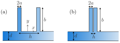
Figure 1: Propagation in a narrow guide loaded by two channels with separation distance of the order of the wavelength (a) or of subwavelength scale (b).

Wave propagation in narrow guides is a practical example of one-dimensional propagation. In this context, resonant scatterers, located inside the guide or attached to its walls, can strongly modify the propagation of the guided waves. When the scatterers are distributed periodically along the guide with spacing about half-wavelength, resonant Bragg interference take place which can be tuned close to the local scatterer resonance Tekman and Bagwell (1993); Kushwaha et al. (1998); El Boudouti et al. (2008); Kaina et al. (2013); Theocharis et al. (2014); Santillán and Bozhevolnyi (2014); Merkel et al. (2015); Leclaire et al. (2015). The appearance, within the Bragg band-gap, of a propagating branch resulting in acoustically induced transparency (AIT) has been studied in detail and the associated Fano resonance has been characterized, see e.g. El Boudouti et al. (2008). More recently, directly or strongly coupled resonators have been shown able to produce similar transparency window attributed to the classical analog of Autler-Townes splitting (ATS) Anisimov et al. (2011); Peng et al. (2014); Jin et al. (2018); Liu et al. (2019); Cheng et al. (2019); Wang et al. (2021). AIT is due to destructive interference of the waves propagating back and forth between the two scatterers. In contrast ATS does not involve propagating waves as the scatterers are directly coupled via the evanescent field.

We consider two narrow channels with closed ends supporting quarter-wavelength resonance attached to one wall of the main waveguide (figure 1). When the distance between the channels is of the order of the wavelength (or greater), the propagation in the guide is well described by a one-dimensional model in which the effect of each channel is encoded in jump conditions across the channel junction. Accounting for the effect of the evanescent field in the junction region improves the accuracy of the model by modifying the form of the jump conditions Wang et al. (2014, 2018); Červenka and Bednařík (2018). So far, this approach has not been adapted to the case where the two channels are so close that they can couple directly through the evanescent field. We provide such a model using asymptotic analysis in the low frequency regime. To stress the difference between the two situations, we first revisit the classical case for large separation distances between the channel junctions. We show that the jump conditions are obtained by considering a locally-incompressible region governed by Laplace’s equation. This problem is solved exactly by exploiting a conformal mapping which provides an explicit expression of the added length in two-dimensions in excellent agreement with previous estimates Červenka and Bednařík (2018); Červenka et al. (2019). We then extend this analysis to the case where the junction includes two channels with subwavelength separation distance.

The paper is organized as follows. In §II the derivation of the two models is presented resulting in the jump conditions (14) and (15). The scattering by a single channel is presented in §III and this provides an important reference to our discussion relating to the scattering by a set of two channels, see §IV. We can already note that for large separation distance $h$ (termed model a) neglecting the effect of the evanescent field in the transition conditions provides reasonable predictions since the resonant mechanism of AIT is captured El Boudouti et al. (2008); Chesnel and Nazarov (2018). In contrast, the strong evanescent field excited in the junction region of two close channels (termed model b) is the basis of the dipolar resonance involved in the ATS. Finally, we envisage in §V a situation involving both resonances using scatterers comprised of a pair of close channels. The Appendices contain additional modelling information, including the derivation of the parameters entering  in the model a and which are found using a conformal mapping. In the study, the results of the effective models are compared with direct numerics based on a multimodal method similar to that used in Maurel et al. (2019).

II The effective models

In this section, we provide the derivation of two different models whose range of validity depends on the separation distance, $h$, between the two channels. To set the scene, we aim to model the perfect transmission illustrated in figure 2(a) for $h/2a\sim 1$ and $h/2a\sim 25$ in the reported example. We notice that perfect transmission is associated with large field amplitudes within the channels being either in-phase for large $h$ (panel (b)) or out-of-phase for small $h$ (panel (c)).

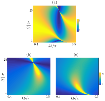
Figure 2: (a) Transmission in the main guide against non-dimensional frequency $kb/\pi$ and separation distance $h/2a$ ($b=d=20a$). (b) Sum and (c) difference of the field amplitudes at the top of the channels.

The jump conditions are obtained using matched asymptotic expansions which requires general solutions in the guide and in the side channels which capture the dominant far-field behaviour of the narrow side channel opening. The approximation to the solution in the guide and in the side channel far away from the channel opening (the junction) is elementary. The most challenging part is the inner region in the vicinity of the junction region. The two models differ since in the model a the junction includes the effect of a single channel while in the model b the junction includes the effect of the pair of side channels, see figure 3.

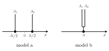
Figure 3: The two one-dimensional models : model a for $kh=O(1)$ resulting in jump conditions (14) at two junctions $x_{\text{\tiny J}}=\pm h/2$, and model b for $kh\ll 1$ resulting in jump conditions (15) at a single junction $x_{\text{\tiny J}}=0$.

II.1 Solution far from the junction

The problem is governed by the Helmholtz equation $\Delta\Phi+k^{2}\Phi=0$ for $\Phi(x,y)$. In the main channel far away from the opening at $x=0$, we shall only need that the solution can be approximated by $\Phi(x,y)\simeq\varphi(x)$ governed by $\varphi^{\prime\prime}(x)+k^{2}\varphi(x)=0$. We note that

$$\varphi(x)\underset{kx\to kx_{\text{\tiny J}}}{\sim}\varphi(x_{\text{\tiny J}}^{\pm})+(x-x_{\text{\tiny J}})\varphi^{\prime}(x_{\text{\tiny J}}^{\pm}).$$ (1)

Similarly, in the $n$th side-channel, $n=1,2$, far away from the opening, we have $\Phi(x,y)\approx\phi_{n}(y)$ governed by $\phi^{\prime\prime}_{n}(y)+k^{2}\phi_{n}(y)=0$, and we note that

$$\phi_{n}(y)\underset{ky\to 0}{\sim}\phi_{n}(0)+y\phi_{n}^{\prime}(0).$$ (2)

II.2 Derivation of the jump conditions

We define

$$\overline{\varphi}=\frac{1}{2}\left(\varphi^{+}+\varphi^{-}\right),\qquad[\varphi]=\left(\varphi^{+}-\varphi^{-}\right)$$

to be the average and the jump of $\varphi$ across the junction at $x=x_{\text{\tiny J}}$ ($\varphi^{\pm}=\varphi(x_{\text{\tiny J}}^{\pm})$). Also, we denote $\theta=a/d$.

II.2.1 Solution in the junction region with a single channel

In the vicinity of the junction between the guide and the channel, we rescale variables on $d$ with

$$x-x_{\text{\tiny J}}=d{\mathsf{x}},\qquad y=d{\mathsf{y}}.$$

Accordingly we set $\Phi(x,y)\simeq\Psi({\mathsf{x}},{\mathsf{y}})$ which, under the working assumption that $kd\ll 1$, approximates the Helmholtz equation as the Laplace equation

$$\nabla^{2}\Psi=0.$$ (3)

We shall now use that the velocity $\nabla\Psi$ at the local scale has to match the velocities in the guide when $kx\to kx_{\text{\tiny J}}^{\pm}$ and in each channel when $ky\to 0$. Specifically, we must have

$$\left\{\begin{array}[]{l}\nabla\Psi\underset{{\mathsf{x}}\to\pm\infty}{\sim}d\varphi^{\prime}(x_{\text{\tiny J}}^{\pm})\,{\bm{e}}_{x}=d\left(\overline{\varphi^{\prime}}\pm\frac{1}{2}[\varphi^{\prime}]\right){\bm{e}}_{x},\vspace{.2cm}\\ \nabla\Psi\underset{{\mathsf{y}}\to+\infty}{\sim}d\phi_{1}^{\prime}(0)\,{\bm{e}}_{y}=-\frac{{\bm{e}}_{y}}{2\theta}\,d[\varphi^{\prime}],\end{array}\right.$$ (4)

where ${\mathsf{x}}\to\pm\infty$ means ${\mathsf{x}}\to\pm\infty$ in the guide and ${\mathsf{y}}\to+\infty$ means ${\mathsf{y}}\to+\infty$ in the channel. In (4), we have used that $[\varphi^{\prime}]+2\theta\phi_{1}^{\prime}(0)=0$. This relation corresponds to the continuity of the flux which arises from integrating (3) and applying the divergence theorem to $\nabla\Psi$.

The system (3-4) is linear with respect to $\overline{\varphi^{\prime}}$ and $[\varphi^{\prime}]$, from which we deduce that $\Psi$ can be sought of the form

$$\Psi({\mathsf{x}},{\mathsf{y}})=d\overline{\varphi^{\prime}}\;\psi({\mathsf{x}},{\mathsf{y}})-\frac{d}{2}[\varphi^{\prime}]\;\psi_{\text{\tiny s}}({\mathsf{x}},{\mathsf{y}})+C,$$ (5)

where $\psi$ and $\psi_{\text{\tiny s}}$ are elementary problems, sketched in figure 4, satisfying the Laplace equation (3) and with the following asymptotic behaviour

$$\left\{\begin{array}[]{ll}\psi\underset{{\mathsf{x}}\to\pm\infty}{\sim}{\mathsf{x}}\pm{\cal A}/2,&\psi\underset{{\mathsf{y}}\to+\infty}{\sim}0,\\ \psi_{\text{\tiny s}}\underset{{\mathsf{x}}\to\pm\infty}{\sim}\mp{\mathsf{x}},&\psi_{\text{\tiny s}}\underset{{\mathsf{y}}\to+\infty}{\sim}\frac{{\mathsf{y}}}{\theta}+{\cal A}_{\text{\tiny s}},\end{array}\right.$$ (6)

($\psi$ and $\psi_{\text{\tiny s}}$ are defined up to constants and we have chosen an antisymmetric form for $\psi$ and a symmetric form for $\psi_{\text{\tiny s}}$). In the above, the parameters $({\cal A},{\cal A}_{\text{\tiny s}})$ which depend on $\theta$ only are to be determined.

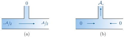
Figure 4: Elementary problems of potential flows with (6) set on (a) $\psi$ and (b) $\psi_{\text{\tiny s}}$.

We now identify (5) for ${\mathsf{x}}\to\pm\infty$ with (1) for $|x-x_{\text{\tiny J}}|\to 0$, and (5) for ${\mathsf{y}}\to+\infty$ with (2) for $y\to 0$. In doing so, we obtain

$$\varphi(x_{\text{\tiny J}}^{\pm})=\pm\frac{{\cal A}}{2}\,d\overline{\varphi^{\prime}}+C,\quad\phi_{1}(0)=-\frac{{\cal A}_{\text{\tiny s}}}{2}\,d[\varphi^{\prime}]+C,$$

and eliminating $C$ from the above expressions,

$$\left\{\begin{array}[]{l}\displaystyle[\varphi]={\cal A}\,d\overline{\varphi^{\prime}},\vspace{.1cm}\\ \displaystyle\phi_{1}(0)-\overline{\varphi}={\cal A}_{\text{\tiny s}}\,a\phi_{1}^{\prime}(0),\vspace{.1cm}\\ \displaystyle d[\varphi^{\prime}]+2a\phi_{1}^{\prime}(0)=0.\end{array}\right.$$ (7)

The jump conditions (7) are the main results of our analysis. They apply whatever channel lengths and end conditions are applied (provided the underlying assumptions that $kd,ka\ll 1$ are maintained). Besides, the parameters $({\cal A},{\cal A}_{\text{\tiny s}})$ are explicit (see appendix A), specifically

$$\left\{\begin{array}[]{l}{\cal A}=\frac{2}{\pi}\left(\log(1+\theta^{2})-2\theta\tan^{-1}\theta\right),\vspace{.2cm}\\ {\cal A}_{\text{\tiny s}}=\frac{2}{\pi}\left(\log\frac{(1+\theta^{2})}{4\theta}+(1/\theta-\theta)\tan^{-1}\theta\right).\end{array}\right.$$ (8)

II.2.2 Solution in the junction region with two channels

When the distance between two channels is subwavelength, the junction contains both side channel openings. We repeat the same exercice as previously with now, the conservation of the flux being $[\varphi^{\prime}]+2\theta(\phi_{1}^{\prime}(0)+\phi^{\prime}_{2}(0))=0$. Also, for convenience, we define

$$\phi_{\text{\tiny s}}=\phi_{1}+\phi_{2},\qquad\phi_{\text{\tiny a}}=\phi_{1}-\phi_{2},$$ (9)

being the symmetric and antisymmetric fields in the channels. The matching conditions on $\nabla\Psi$ read

$$\left\{\begin{array}[]{l}\nabla\Psi\underset{{\mathsf{x}}\to\pm\infty}{\sim}d\varphi^{\prime}(x_{\text{\tiny J}}^{\pm}){\bm{e}}_{x}=d\left(\overline{\varphi^{\prime}}\pm\frac{1}{2}[\varphi^{\prime}]\right){\bm{e}}_{x},\vspace{.2cm}\\ \nabla\Psi\underset{{\mathsf{y}}\to+\infty_{1}}{\sim}d\phi_{1}^{\prime}(0){\bm{e}}_{y}=-\frac{{\bm{e}}_{y}}{4\theta}\,d[\varphi^{\prime}]+\frac{{\bm{e}}_{y}}{2}\,d\phi_{\text{\tiny a}}^{\prime}(0),\vspace{.2cm}\\ \nabla\Psi\underset{{\mathsf{y}}\to+\infty_{2}}{\sim}d\phi_{2}^{\prime}(0){\bm{e}}_{y}=-\frac{{\bm{e}}_{y}}{4\theta}\,d[\varphi^{\prime}]-\frac{{\bm{e}}_{y}}{2}\,d\phi_{\text{\tiny a}}^{\prime}(0).\end{array}\right.$$ (10)

The system (3) with (10) is linear with respect to $\overline{\varphi^{\prime}}$, $[\varphi^{\prime}]$ and $\phi_{\text{\tiny a}}^{\prime}(0)$ from which we deduce that $\Psi$ can be sought of the form

$$\Psi=d\overline{\varphi^{\prime}}\;\psi-\frac{d[\varphi^{\prime}]}{2}\;\psi_{\text{\tiny s}}+a\phi_{\text{\tiny a}}^{\prime}(0)\,\psi_{\text{\tiny a}}+C,$$ (11)

with $\psi$, $\psi_{\text{\tiny s}}$ and $\psi_{\text{\tiny a}}$ satisfying the Laplace equation and with the following asymptotic behaviours

$$\left\{\begin{array}[]{l}\psi\underset{{\mathsf{x}}\to\pm\infty}{\sim}{\mathsf{x}}\pm{\cal B}/2,\quad\psi\underset{{\mathsf{y}}\to\infty_{1}}{\sim}-\hat{\cal B}_{\text{\tiny a}}/2,\quad\psi\underset{{\mathsf{y}}\to\infty_{2}}{\sim}\hat{\cal B}_{\text{\tiny a}}/2,\vspace{.3cm}\\ \begin{array}[]{ll}\psi_{\text{\tiny s}}\underset{{\mathsf{x}}\to\pm\infty}{\sim}\mp{\mathsf{x}},&\psi_{\text{\tiny s}}\underset{{\mathsf{y}}\to+\infty_{1}}{\sim}\frac{{\mathsf{y}}}{2\theta}+{\cal B}_{\text{\tiny s}}/2,\\ &\psi_{\text{\tiny s}}\underset{{\mathsf{y}}\to+\infty_{2}}{\sim}\frac{{\mathsf{y}}}{2\theta}+{\cal B}_{\text{\tiny s}}/2,\vspace{.3cm}\\ \psi_{\text{\tiny a}}\underset{{\mathsf{x}}\to\pm\infty}{\sim}\mp\hat{\cal B}_{\text{\tiny a}}/2,&\psi_{\text{\tiny a}}\underset{{\mathsf{y}}\to+\infty_{1}}{\sim}\pm\frac{{\mathsf{y}}}{2\theta}\pm{\cal B}_{\text{\tiny a}}/2,\\ &\psi_{\text{\tiny a}}\underset{{\mathsf{y}}\to+\infty_{2}}{\sim}\pm\frac{{\mathsf{y}}}{2\theta}\pm{\cal B}_{\text{\tiny a}}/2,\end{array}\end{array}\right.$$

(${\mathsf{y}}\to+\infty_{1}$ means ${\mathsf{y}}\to+\infty$ in the first channel, ${\mathsf{y}}\to+\infty_{2}$ means ${\mathsf{y}}\to+\infty$ in the second channel).

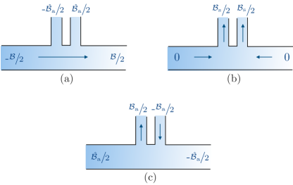
Figure 5: Elementary problems of potential flows with (10) set on (a) $\psi$, (b) $\psi_{\text{\tiny s}}$ and (c) $\psi_{\text{\tiny a}}$.

Note that the parameters ${\cal B}$ and ${\cal B}_{\text{\tiny s}}$ are associated with similar elementary problems as those appearing for a single channel, see (a) and (b) in figures 4 and 5. In contrast the parameters ${\cal B}_{\text{\tiny a}}$ and $\hat{\cal B}_{\text{\tiny a}}$ are associated with a new antisymmetric problem involving the exchange of flux between the two channels (which was obviously not possible for a single channel). The parameter $\hat{\cal B}_{\text{\tiny a}}$ appears in the two problems on $\psi$ and $\psi_{\text{\tiny a}}$; indeed, integrating by part the product $\psi\Delta\psi_{\text{\tiny a}}=0$, we obtain $\hat{\cal B}_{\text{\tiny a}}=-\int\nabla\psi\nabla\psi_{\text{\tiny a}}$ using that $\psi{\sim}\mp\hat{\cal B}_{\text{\tiny a}}/2$ for ${\mathsf{y}}\to\infty$ in the channels; in doing the same for $\psi_{\text{\tiny a}}\Delta\psi=0$, we obtain $\hat{\cal B}_{\text{\tiny a}}=-\int\nabla\psi\nabla\psi_{\text{\tiny a}}$ using that $\psi_{\text{\tiny a}}{\sim}\mp\hat{\cal B}_{\text{\tiny a}}/2$ for ${\mathsf{x}}\to\pm\infty$ in the guide.

As for a single channel, we now identify (11) for ${\mathsf{x}}\to\pm\infty$ with (1) for $|x-x_{\text{\tiny J}}|\to 0$, and (11) for ${\mathsf{y}}\to+\infty_{n}$, $n=1,2$ with (2) for $y\to 0$ in the first channel and in the second channel. This results in

$$\begin{array}[]{l}\varphi(0^{\pm})=\pm\frac{{\cal B}}{2}\,d\overline{\varphi^{\prime}}\mp\frac{\hat{\cal B}_{\text{\tiny a}}}{2}a\phi_{\text{\tiny a}}^{\prime}(0)+C,\vspace{.1cm}\\ \phi_{1}(0)=-\frac{\hat{\cal B}_{\text{\tiny a}}}{2}d\overline{\varphi^{\prime}}-\frac{{\cal B}_{\text{\tiny s}}}{2}\frac{d[\varphi^{\prime}]}{2}+\frac{{\cal B}_{\text{\tiny a}}}{2}a\phi_{\text{\tiny a}}^{\prime}(0)+C,\vspace{.1cm}\\ \phi_{2}(0)=\frac{\hat{\cal B}_{\text{\tiny a}}}{2}d\overline{\varphi^{\prime}}-\frac{{\cal B}_{\text{\tiny s}}}{2}\frac{d[\varphi^{\prime}]}{2}-\frac{{\cal B}_{\text{\tiny a}}}{2}a\phi_{\text{\tiny a}}^{\prime}(0)+C,\end{array}$$

and thus

$$\left\{\begin{array}[]{l}\displaystyle[\varphi]={\cal B}\,d\overline{\varphi^{\prime}}-\hat{\cal B}_{\text{\tiny a}}\,a\phi_{\text{\tiny a}}^{\prime}(0),\vspace{.1cm}\\ \displaystyle\phi_{\text{\tiny s}}=2\overline{\varphi}+{\cal B}_{\text{\tiny s}}\,a\phi_{\text{\tiny s}}^{\prime},\quad\displaystyle\phi_{\text{\tiny a}}=-\hat{\cal B}_{\text{\tiny a}}\,d\overline{\varphi^{\prime}}+{\cal B}_{\text{\tiny a}}\,a\phi_{\text{\tiny a}}^{\prime},\vspace{.1cm}\\ \displaystyle d[\varphi^{\prime}]+2a\phi_{\text{\tiny s}}^{\prime}=0.\end{array}\right.$$ (12)

The jump conditions (12) are the jump conditions produced by two channels with subwavelength distance (as opposed to (7)). As for a single channel, they apply whatever the heights of the two channels and whatever the end conditions are (and the heights and end conditions of the two channels can be different).

II.3 The final models

The final models are now written considering that the channels have closed ends at $y=b$, hence

$$\phi_{n}(y)=A_{n}\frac{\cos k(y-b)}{\cos kb},\quad n=1,2.$$ (13)

In the model a for a single channel, we thus have $\phi_{1}(0)=A_{1}$ and $\phi_{1}^{\prime}(0)=A_{1}k\tan kb$ which can be used in (7) to determine the jump conditions applying on $\varphi$ only, after eliminating $A_{1}$. They read

$$\left\{\begin{array}[]{l}\displaystyle d[\varphi^{\prime}]=\alpha_{\text{\tiny s}}\overline{\varphi},\quad[\varphi]=\alpha_{\text{\tiny a}}\,d\overline{\varphi^{\prime}},\vspace{.3cm}\\ \alpha_{\text{\tiny s}}=\frac{2{\mathsf{x}}}{{\cal A}_{\text{\tiny s}}{\mathsf{x}}-1},\qquad\alpha_{\text{\tiny a}}={\cal A},\end{array}\right.$$ (14)

where ${\mathsf{x}}=ka\tan kb$. Once $\varphi(x)$ has been obtained, $A_{1}$ can be determined from (7). In the model b, (13) applies to $\varphi_{\text{\tiny s}}$ and $\varphi_{\text{\tiny a}}$ with $A_{\text{\tiny s}}=(A_{1}+A_{2})$, $A_{\text{\tiny a}}=(A_{1}-A_{2})$, from (9). Eliminating $A_{\text{\tiny s}}$ and $A_{\text{\tiny a}}$ in (12) yields

$$\left\{\begin{array}[]{l}d[\varphi^{\prime}]=\beta_{\text{\tiny s}}\overline{\varphi},\quad[\varphi]=\beta_{\text{\tiny a}}\,d\overline{\varphi^{\prime}}.\vspace{.3cm}\\ \beta_{\text{\tiny s}}=\frac{4{\mathsf{x}}}{{\cal B}_{\text{\tiny s}}{\mathsf{x}}-1},\qquad\beta_{\text{\tiny a}}={\cal B}-\frac{\hat{\cal B}_{\text{\tiny a}}^{2}{\mathsf{x}}}{{\cal B}_{\text{\tiny a}}{\mathsf{x}}-1}.\end{array}\right.$$ (15)

Eventually, once $\varphi(x)$ has been obtained, $(A_{\text{\tiny s}},A_{\text{\tiny a}})$ (and $(A_{1},A_{2})$) can be obtained from (12) (and (9)).

III Scattering by a single channel

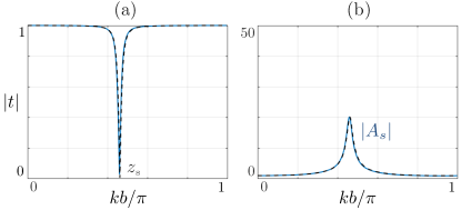
Figure 6: (a) Transmission $|t|$ by a single channel and (b) amplitude $|A_{\text{\tiny s}}|$ at the top of the channel (here $A_{\text{\tiny s}}=A_{1}$) against the non-dimensional frequency $kb/\pi$ ($d=b=20a$). Direct numerics (plain lines) and from (16) (dashed black lines).

To begin with, we consider a single channel opening onto the main guide at $x=0$. The features of this problem will provide an important guide to the discussion of two channels. For an incident right-going wave, we look for a solution $\varphi(x)$ of the form

$$\left\{\begin{array}[]{ll}\displaystyle\varphi(x)=e^{ikx}+re^{-ikx},&x\in(-\infty,0),\\ \displaystyle\varphi(x)=te^{ikx},&x\in(0,+\infty),\end{array}\right.$$

with the jump conditions (14) at $x_{\text{\tiny J}}=0$. We obtain

$$\left\{\begin{array}[]{ll}\displaystyle r=\frac{1}{2}\left(\frac{{\mathrm{y}}_{\text{\tiny s}}}{{\mathrm{y}}_{\text{\tiny s}}^{*}}-\frac{{\mathrm{y}}_{\text{\tiny a}}}{{\mathrm{y}}_{\text{\tiny a}}^{*}}\right),&\displaystyle t=\frac{1}{2}\left(\frac{{\mathrm{y}}_{\text{\tiny s}}}{{\mathrm{y}}_{\text{\tiny s}}^{*}}+\frac{{\mathrm{y}}_{\text{\tiny a}}}{{\mathrm{y}}_{\text{\tiny a}}^{*}}\right),\vspace{.2cm}\\ \displaystyle{\mathrm{y}}_{\text{\tiny s}}=1-\frac{i\alpha_{\text{\tiny s}}}{2kd},&\displaystyle{\mathrm{y}}_{\text{\tiny a}}=1+\frac{ikd\alpha_{\text{\tiny a}}}{2},\end{array}\right.$$ (16)

with $(\alpha_{\text{\tiny s}},\alpha_{\text{\tiny a}})$ defined in (14) along with (8). As it should be, the scattering coefficients satisfies the energy conservation $|r|^{2}+|t|^{2}=1$ and the reciprocity $rt^{*}+tr^{*}=0$. The figure 6 shows the transmission $|t|$ and the amplitude $A_{1}=\alpha_{\text{\tiny s}}/({\mathsf{x}}{\mathrm{y}}_{\text{\tiny s}}^{*})$ at the top of the channel for $d=b=20a$.

The effect of this thin channel is in general weak (hence $|t|\simeq 1$) except at the quarter-wavelength resonance for $kb\simeq\pi/2$ which produces a zero-transmission ($z_{\text{\tiny s}}$). From (16) this first zero-transmission corresponds to $\text{cot}kb_{\text{\tiny eff}}=0$ with $b_{\text{\tiny eff}}$ the so-called effective length given by

$$\begin{array}[]{l}k_{0}=\frac{\pi}{2b_{\text{\tiny eff}}},\qquad b_{\text{\tiny eff}}=(b+b_{\text{\tiny add}}),\vspace{.2cm}\\ b_{\text{\tiny add}}=\frac{2}{\pi}\left(\frac{1}{\theta}\tan^{-1}\theta-\log\left(\frac{4\theta}{\sqrt{1+\theta^{2}}}\right)\right)\;a.\end{array}$$ (17)

The variation of $k_{0}$ against $d/a$ is manifested in the zero of $|T|$ in the $(kb/\pi,d/2a)$ plane in figure 7(b) (the dashed white line shows $k_{0}$ in (17); the relative error w.r.t. the numerics is less than 0.05% up to $d/2a=5$ afterwards it increases slightly, up to 0.3% at $d/2a$=10). We did not find a similar theoretical prediction for the added length in the literature. However, we notice the good agreement between (17) and the fits proposed in Červenka and Bednařík (2018); Červenka et al. (2019) resulting in $\frac{b_{\text{\tiny add}}}{2a}=0.52$ for $\theta=\frac{2}{15}$ ((17) provides $\frac{b_{\text{\tiny add}}}{2a}=0.5193$).

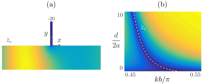
Figure 7: (a) Real part of the field at the resonance of a single channel, (b) Transmission coefficient $|t|$ from direct numerics against non-dimensional frequency $kb/\pi$ and non-dimensional guide width $d/2a$. The dashed white line shows $k_{0}$ from (17).

Finally, and anticipating an easier comparison with the case of two channels, we provide an approximate expression of $t$ in (16) close to the resonance for $kb_{\text{\tiny eff}}=\frac{\pi}{2}+\varepsilon$, $\varepsilon\ll 1$ (hence ${\mathsf{x}}\simeq-\frac{\pi a}{2b_{\text{\tiny eff}}\varepsilon}$ in (14)). In doing so, we obtain

$$t=\frac{(k-k_{0})}{(k-k_{\text{\tiny s}})},\quad k_{\text{\tiny s}}=k_{0}-i\frac{\theta}{b},$$ (18)

with $k_{0}$, in (17), the wavenumber at zero-transmission.

IV Close channels or far channels, two different resonant mechanisms

IV.1 Far channels, AIT in the classical model a

In the classical model a, the evanescent fields are confined to the vicinity of each channel with no overlap. Hence, the solution is sought in the form

$$\left\{\begin{array}[]{ll}\displaystyle\varphi(x)=e^{ikx}+Re^{-ikx},&x\in(-\infty,-h/2),\vspace{.1cm}\\ \displaystyle\varphi(x)=G_{\text{\tiny s}}\cos kx+G_{\text{\tiny a}}\sin kx,&x\in(-h/2,h/2),\vspace{.1cm}\\ \displaystyle\varphi(x)=Te^{ikx},&x\in(h/2,+\infty),\end{array}\right.$$ (19)

with (14) applying at $x_{\text{\tiny J}}=\pm h/2$. It follows that

$$\left\{\begin{array}[]{l}\displaystyle R=\frac{1}{2}\left(\frac{Z_{\text{\tiny s}}}{Z_{\text{\tiny s}}^{*}}-\frac{Z_{\text{\tiny a}}}{Z_{\text{\tiny a}}^{*}}\right),\quad\displaystyle T=\frac{1}{2}\left(\frac{Z_{\text{\tiny s}}}{Z_{\text{\tiny s}}^{*}}+\frac{Z_{\text{\tiny a}}}{Z_{\text{\tiny a}}^{*}}\right),\vspace{.4cm}\\ \displaystyle Z_{\text{\tiny s}}=(1+i\text{t})\left(1+\frac{\alpha_{\text{\tiny a}}\alpha_{\text{\tiny s}}}{4}\right)-i\frac{\alpha_{\text{\tiny s}}}{kd}-\alpha_{\text{\tiny a}}kd\,\text{t},\vspace{.3cm}\\ \displaystyle Z_{\text{\tiny a}}=(1+i\text{t})\left(1+\frac{\alpha_{\text{\tiny a}}\alpha_{\text{\tiny s}}}{4}\right)+\frac{\alpha_{\text{\tiny s}}}{kd}\text{t}+i\alpha_{\text{\tiny a}}kd,\end{array}\right.$$ (20)

where $\text{t}=\tan(kh/2)$.

The transmission spectrum given by (20) in the model a is shown in figure 8 to be compared to that calculated numerically (the same as in figure 2(a)). As expected, when the two channels have large separation distance $h$, the interaction between them (when they interact) is attributable to interference of propagating waves, hence the model a, which is the classical model, is valid.

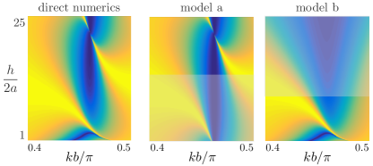
Figure 8: Comparison of the transmission spectra given by direct numerics and given by the model a, from (20) and by the model b, from (24). The grey regions hide the region where each model is not valid ($d=b=20a$).

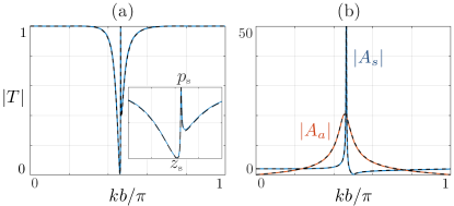
Figure 9: (a) Transmission against $kb/\pi$; the inset shows the range $kb/2\pi\in(0.42,0.5)$ (b) Symmetric $A_{\text{\tiny s}}$ and antisymmetric $A_{\text{\tiny a}}$ amplitudes ($h=2b$ and $b=d=20a$). Direct numerics (plain lines) and from (20) (dashed black lines).

We provide quantitative comparisons in figure 9 where we report the variations of $|T|$ and of $(A_{\text{\tiny s}},A_{\text{\tiny a}})$ for $h=20a$. The transmission resembles that obtained for a single channel except for the occurrence of a perfect transmission (named $p_{\text{\tiny s}}$) following the zero-transmission $z_{\text{\tiny s}}$, a feature characteristic of Fano resonance and which is accurately captured by the model. The shape of the quasi-trapped associated with the Fano resonance is visible at $p_{\text{\tiny s}}$ in figure 10.

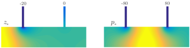
Figure 10: Real parts of the fields at the zero-transmission ($z_{\text{\tiny s}}$) and at the perfect transmission ($p_{\text{\tiny s}}$) revealing the shape of the symmetric quasi-trapped mode.

The complex poles of the Fano resonance and the associated perfect- or quasi-trapped modes have been analyzed in several studies see, e.g.  Chesnel and Nazarov (2018). Our effective model provides approximate expressions of these poles owing to expansions of the scattering coefficients in the vicinity of $kb_{\text{\tiny eff}}=\pi/2$ as we have done for a single channel. We define the detuning parameter $\delta$ as

$$\delta=\pi\left(\frac{h}{2b_{\text{\tiny eff}}}-1\right),$$

hence for $\delta=0$, the Bragg and the quarter-wavelength resonances are perfectly tuned. From (20), we obtain

$$T\simeq\frac{(k-k_{0})^{2}}{(k-k^{+})(k-k^{-})},$$ (21)

with $k_{0}$ defined in (17) and

$$\begin{array}[]{l}\displaystyle k^{-}=k_{0}+\frac{\theta\delta}{b_{\text{\tiny eff}}}-i\frac{2\theta}{b_{\text{\tiny eff}}},\quad\displaystyle k^{+}=k_{0}-\frac{\theta\delta}{b_{\text{\tiny eff}}}-i\frac{\theta\delta^{2}}{2b_{\text{\tiny eff}}}.\end{array}$$ (22)

The two poles are dictated by the detuning parameter with the pole $k^{-}$ relating to a weak resonance corresponding roughly to the pole of a single channel of width $4a$ and the pole $k^{+}$ relating to the strong resonance associated with the quasi-trapped mode resonance. In particular, when $\delta=0$, $k^{+}=k_{0}$ becomes real, the quasi-trapped mode becomes a perfect-trapped mode and the Fano resonance disappears.

IV.2 Close channels, the model b

Contrary to the model a, model b concerns the case where the channels are close enough that the evanescent field in the junction region plays a leading order effect in connecting the two channels. This is accounted for in the model b by reducing the region of the two channels to a single junction. Accordingly, we look for a solution $\varphi(x)$

$$\left\{\begin{array}[]{ll}\displaystyle\varphi(x)=e^{ikx}+Re^{-ikx},&x\in(-\infty,0),\\ \displaystyle\varphi(x)=Te^{ikx},&x\in(0,+\infty),\end{array}\right.$$ (23)

and we apply the jump conditions (15) at the single junction $x_{\text{\tiny J}}=0$. The resulting scattering coefficients hence read

$$\left\{\begin{array}[]{ll}\displaystyle R=\frac{1}{2}\left(\frac{Y_{\text{\tiny s}}}{Y_{\text{\tiny s}}^{*}}-\frac{Y_{\text{\tiny a}}}{Y_{\text{\tiny a}}^{*}}\right),&\displaystyle T=\frac{1}{2}\left(\frac{Y_{\text{\tiny s}}}{Y_{\text{\tiny s}}^{*}}+\frac{Y_{\text{\tiny a}}}{Y_{\text{\tiny a}}^{*}}\right),\vspace{.2cm}\\ \displaystyle Y_{\text{\tiny s}}=1-\frac{i\beta_{\text{\tiny s}}}{2kd},&\displaystyle Y_{\text{\tiny a}}=1+\frac{ikd\beta_{\text{\tiny a}}}{2},\end{array}\right.$$ (24)

with $(\beta_{\text{\tiny s}},\beta_{\text{\tiny a}})$ in (15). It is worth noticing that the effect of $h$ is now entirely encapsulated in the effective parameters $({\cal B}_{\text{\tiny s}},{\cal B}_{\text{\tiny a}},\hat{\cal B}_{\text{\tiny a}})$. Furthermore, neglecting the evanescent field (resulting in $\beta_{\text{\tiny s}}=-4{\mathsf{x}}$ and $\beta_{\text{\tiny a}}=0$ in (15)) would completely fail in predicting the observed spectrum. Indeed, doing so would reduce the two channels to a single one.

To begin with, we come back to the figure 8 where, in panel (c), we showed the transmission spectrum given by (24). As expected, model b is valid only for small distances, $h$, which include the region of the Autler-Townes splitting. Eventually, the model a (resp. b) is valid for $h/2a\gtrsim 7$ (resp. $h/2a\lesssim 7$). This corresponds to $kh\sim 1$ which is consistent with the asymptotic analysis presented in §II. The accuracy of the model b is further illustrated in figure 11 where we report $|T|$ and $(A_{\text{\tiny s}},A_{\text{\tiny a}})$ against the non-dimensional frequency for $h=a$ (the two channels are contiguous). The resonance due to ATS is associated with a strong dipolar behaviour of the two channels, able to produce a zero-transmission (named $z_{\text{\tiny a}}$) immediately followed by a perfect-transmission (named $p_{\text{\tiny a}}$). The corresponding patterns are shown in figure 12 where we see the strong evanescent field inducing a dipolar behaviour in the vicinity of the channel openings.

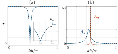
Figure 11: Transmission $|T|$ and amplitudes $(A_{\text{\tiny s}},A_{\text{\tiny a}})$, same representation as in figure 9 for $h=a$ ($b=d=20a$); the maximum of $A_{\text{\tiny a}}$ is at about 300.

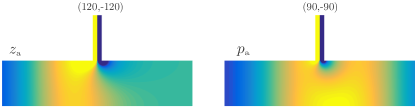
Figure 12: Real part of the fields at the zero-transmission $z_{\text{\tiny a}}$ and the perfect-transmission $p_{\text{\tiny a}}$ associated with the dipolar behavior of the pair of contiguous channels.

Contrary to the case of the Fano resonance, the resonance associated with ATS has received much less attention. In Cheng et al. (2019), the dipolar behavior of the ATS resonance has been observed for two Helmholtz resonators (see figure 4 (c-d) in this reference), and the Akaike criterion has been used to discriminate the ATS from the AIT. Close to the resonance at $kb=\pi/2$, and using Taylor expansions as before, we obtain

$$T\simeq\frac{(k-k_{0}^{+})(k-k_{0}^{-})}{(k-k^{+})(k-k^{-})},\quad$$ (25)

with $k_{0}^{\pm}$ associated with zero-transmissions given by

$$k_{0}^{\pm}-k_{0}=\pm\frac{\pi a}{2b^{2}}\sqrt{\Delta},$$ (26)

(and $k_{0}$ in (18)) and with the complex poles $k^{\pm}$ given by

$$\left\{\begin{array}[]{l}k^{+}-k_{0}=\frac{\pi a}{2b^{2}}\delta_{r}-2i\frac{\theta}{b}\left(\frac{\pi d}{4b}\hat{\cal B}_{\text{\tiny a}}\right)^{2}\vspace{.2cm}\\ k^{-}-k_{0}=-\frac{\pi a}{2b^{2}}\delta_{r}-2i\frac{\theta}{b},\end{array}\right.$$ (27)

(with $k_{\text{\tiny s}}$ in (18)). In the above, we have defined $\Delta=(\delta_{r}^{2}-\hat{\cal B}_{\text{\tiny a}}^{2})$ and $2\delta_{r}=({\cal B}_{\text{\tiny s}}-{\cal B}_{\text{\tiny a}})$ and we have used that ${\cal B}\simeq 2{\cal A}$ and that $({\cal B}_{\text{\tiny s}}+{\cal B}_{\text{\tiny a}})\simeq 2{\cal A}_{\text{\tiny s}}$; see appendix B.

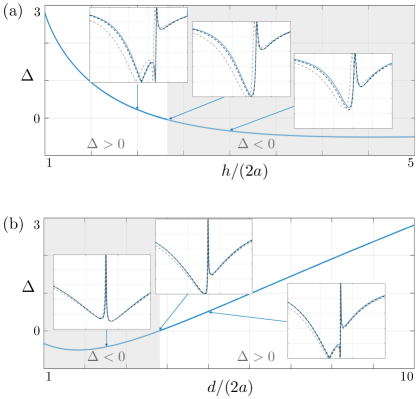
Figure 13: Variations of $\Delta$ in (26) against (a) the non dimensional spacing $h/2a$ ($d=10a$), and (b) the non dimension guide width $d/2a$ ($h=a$) (b). The insets show $|T|$ against $kb/\pi\in(0.4,0.5)$ in (a) and $kb/\pi\in(0.4,0.55)$ in (b) from direct numerics (plain lines) from $T$ in (24) (black dashed lines) and its approximate version (25) (grey dashed lines).

The different shapes in the transmission profiles are shown in figure 13 for $\Delta>0$ resulting in two zero-transmissions, $\Delta=0$ resulting in a single zero-transmission and $\Delta<0$ resulting in no zero-transmission. In all cases, the model b captures these variations accurately using $T$ in (24) (dashed black lines) and reasonably using the approximate form in (25) (dashed grey lines).

We have seen that the single zero-transmission of the Fano resonance occurs for $k=k_{0}$, associated with that of a single channel (from (21)). Here, in contrast, the two zero-transmissions are split symmetrically with respect to $k_{0}$ along the real axis when $\Delta>0$ and along the imaginary axis when $\Delta<0$; the same applies for the real parts of two poles. However, the relative positions of the complex parts of the poles depend on the geometry notably through $\hat{\cal B}_{\text{\tiny a}}$. With $k^{-}$ associated with the symmetric solution and $k^{+}$ with the antisymmetric solution, the pole $k^{+}$ is, in general, closer to the real axis. The most striking feature which allows us to eliminate the Fano resonance is that there is no trapped mode when the channel are sufficiently close and this is consistent with the fact that $\hat{\cal B}_{\text{\tiny a}}^{2}>0$ (see appendix B).

We end with a comparison between AIT and ATS and we report in figure 14 the transmission spectrum as the guide width $d/2a$ varies for $h=20a$ and for $h=a$. As a guideline, the dashed white line shows the trajectory of the zero-transmission for a single channel. For (a) $h=20a$, the zero-transmission follows the same path as for a single channel; it is preceded or followed by the perfect transmission resulting in a Fano resonance which disappears at the perfect tuning (white arrow). For (b) $h=a$, the two zero-transmissions result from the splitting of the single channel zero-transmission.

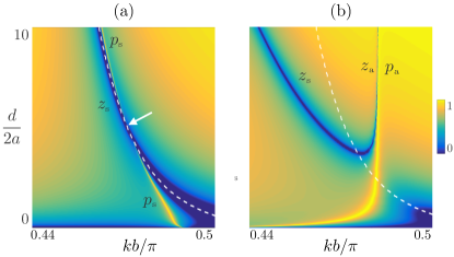
Figure 14: Transmission spectra (in log-scale) against the non-dimensional frequency $kb/\pi$ and the guide width $d/2a$. The dashed white lines show $k_{0}$ associated with zero-transmission for a single channel.

V Scattering by channels with monopolar and dipolar resonances

Owing to the previous analyses for large or subwavelength separation distances, we now consider a combination of channels offering monopolar and dipolar resonances. This is done using two scatterers with spacing $H$ on the scale of the wavelength, each scatterer being composed by two channels with subwavelength separation distance $h$ (figure 15).

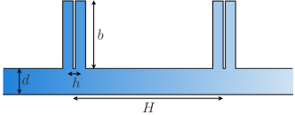
Figure 15: Arrangement of channels able to produce monopolar and dipolar resonances.

The corresponding one-dimensional model is straightforward and it corresponds to a mix of the models a and b. Indeed, we have to consider two junctions with separation distance $H$ as in the model a. Next at each junction (15) applies for a scatterer being composed by a pair of channels. Hence the solution reads as in (19) replacing $h$ by $H$ and $(\alpha_{\text{\tiny s}},\alpha_{\text{\tiny a}})$ by $(\beta_{\text{\tiny s}},\beta_{\text{\tiny a}})$. As a result, the scattering coefficients $({\cal R},{\cal T})$ read

$$\left\{\begin{array}[]{l}\displaystyle{\cal R}=\frac{1}{2}\left(\frac{{\cal Z}_{\text{\tiny s}}}{{\cal Z}_{\text{\tiny s}}^{*}}-\frac{{\cal Z}_{\text{\tiny a}}}{{\cal Z}_{\text{\tiny a}}^{*}}\right),\quad\displaystyle{\cal T}=\frac{1}{2}\left(\frac{{\cal Z}_{\text{\tiny s}}}{{\cal Z}_{\text{\tiny s}}^{*}}+\frac{{\cal Z}_{\text{\tiny a}}}{{\cal Z}_{\text{\tiny a}}^{*}}\right),\vspace{.4cm}\\ \displaystyle{\cal Z}_{\text{\tiny s}}=(1+i\text{t})\left(1+\frac{\beta_{\text{\tiny a}}\beta_{\text{\tiny s}}}{4}\right)-i\frac{\beta_{\text{\tiny s}}}{kd}-\beta_{\text{\tiny a}}kd\text{t},\vspace{.3cm}\\ \displaystyle{\cal Z}_{\text{\tiny a}}=(1+i\text{t})\left(1+\frac{\beta_{\text{\tiny a}}\beta_{\text{\tiny s}}}{4}\right)+\frac{\beta_{\text{\tiny s}}}{kd}\text{t}+i\beta_{\text{\tiny a}}kd,\end{array}\right.$$ (28)

where $\text{t}=\tan(kH/2)$. Figure 16 shows the transmission spectrum by the four channels with $H/2a=20$ and $h/2a=1$ (same representation as in figure 14). We notice the good overall agreement between the direct numerics and the model (28) and this is further illustrated in figure 17 with the profile of $|{\cal T}|$ for $d/2a=10$.

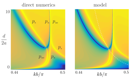
Figure 16: Transmission spectrum for $H/2a=20$, $h/2a=1$ and $b/2a=10$, from direct numerics and from (28).

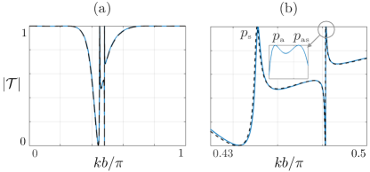
Figure 17: Transmission profile for $d/2a=10$ from direct numerics (plain line) and from (28) (dashed black line), (b) shows a magnification on the two peaks and the inset a magnification on the second transmission peak $kb/\pi\in 0.48170+(0,8.10^{-5})$.

The overall appearance of the spectrum in figure 16 is very similar to that of a single pair of channels reported in figure 14(b) which suggests that the dipolar resonance is more robust than the monopolar one. The branch $p_{\text{\tiny a}}$ is recovered almost unchanged but it is now sandwiched between two branches being the branch $p_{\text{\tiny s}}$ and a new branch that we term $p_{\text{\tiny as}}$.

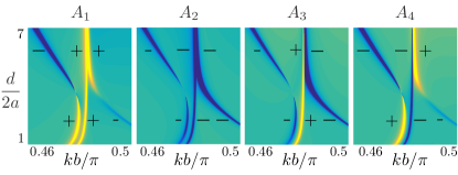
Figure 18: Real parts of the amplitudes $A_{n}$, $n=1,\cdots 4$, at the tops of the 4 channels.

To identify the different branches, we considered the real parts of the amplitudes $A_{n}$, $n=1,\cdots,4$ against non-dimensional frequency and guide width (figure 18). On the central branch, $(A_{1},A_{2},A_{3},A_{4})=(+,-,+,-)$ which means that each pair of channel realizes the perfect-transmission $p_{\text{\tiny a}}$ as if it was alone; this is why we continue to name it $p_{\text{\tiny a}}$. Surrounding this central branch, the side branches experience a kind of avoiding crossing at $d/2a\sim 3.5$. We continue to term $p_{\text{\tiny s}}$ the parts of these branches corresponding to the four channels with in-phase oscillations that is $(A_{1},A_{2},A_{3},A_{4})=(-,-,-,-)$. Indeed, along $p_{\text{\tiny s}}$ the two pairs of channels behave as two single channels of width $4a$ with separation distance $H$. Eventually, $p_{\text{\tiny as}}$ corresponds to $(A_{1},A_{2},A_{3},A_{4})=(\pm,\mp,\mp,\pm)$; this is a new resonance with out-of-phase oscillations of the contiguous channels within a pair, and out-of-phase oscillations of the two pairs. From figure 18, the parts of the side-branches associated with $p_{\text{\tiny s}}$ and $p_{\text{\tiny as}}$ have been identified (see figure 16) and we report in figure 19 the fields at the three perfect-transmissions for $d/2a=3$ and 5. Both $p_{\text{\tiny s}}$ and $p_{\text{\tiny as}}$ are associated with a Fano resonance and, at the perfect tuning, which occurs at $d/2a\simeq 3.5$, they exchange places. Additional results are given in appendix C.

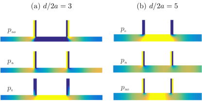
Figure 19: Real parts of the fields at perfect-transmissions $p_{\text{\tiny as}}$, $p_{\text{\tiny a}}$ and $p_{\text{\tiny s}}$; from top to bottom, the frequency is increasing.

We conclude our study with a remark which is evident in light of what has gone before. The model above which mixes models a and b and provides (28) is valid only when $H$ is on the scale of the wavelength. If $H$ becomes subwavelength, the branch $p_{\text{\tiny as}}$ cannot exist since it involves interference between the two pairs of channels. Instead, new branches appear which are associated with resonances of a single scatterer comprised of four contiguous channels. These new arrangements are shown in figure 20.

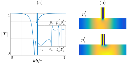
Figure 20: (a) Transmission $|{\cal T}|$ against non dimensional frequency for four contiguous channels; the inset shows the range $kb/2\pi\in(0.42,0.5)$. (b) Real parts of the fields at the perfect transmissions $(p_{\text{\tiny s}}^{\prime},p_{\text{\tiny a}}^{\prime})$ corresponding to the new resonances of the set of four channels.

We recover $z_{\text{\tiny s}}$ when the four channels behave as a single channel of width $8a$ and $(z_{\text{\tiny a}},p_{\text{\tiny a}})$ when the first two and the last two channels behave as a pair of channels of width $4a$. Next, the first new resonance is symmetric with the two central channels and the side channels oscillating out-of-phase. The second new resonance is antisymmetric with the four successive channels oscillating out-of-phase. Each new resonance produces an additional zero- and perfect-transmission $(z_{\text{\tiny s}}^{\prime},p_{\text{\tiny s}}^{\prime})$ and $(z_{\text{\tiny a}}^{\prime},p_{\text{\tiny a}}^{\prime})$.

To account for these new resonances, we should apply the analysis conducted for a set of two channels (model b) to the set of four channels. Such analysis would involve five elementary problems instead of the three sketched in figure 5 (more generally, a set of $N$ channels with subwavelength extend would involve $(N+1)$ elementary problems). Note that the accumulation of resonances for large $N$ while keeping constant the small extend $2Na$ has been considered in Jan and Porter (2018) (see figure 2 in this reference and figure 3 in the associated supplementary report). The succession of transmission profiles in figures 6 ($N=1$), 11 ($N=2$) and 20 ($N=4$) show how this limit would be reached.

VI Conclusion

We have analyzed the scattering of waves in a guide attached to two side channels with quarter-wavelength resonances using the method of matched asymptotic expansions. The asymptotic procedure includes the analysis of a problem of potential flow in a region local to the side-channel junction. Solutions are naturally sensitive to the local geometry at the junction especially whether it contains one or a pair of side channels. It results two different models which are increasingly accurate in the limit of large and small channel separation.

The present analysis applies to analog systems where ATS and EIT have been discussed, including acoustic waves in a guide loaded by Helmholtz resonators Cheng et al. (2019), elastic guided waves such as Lamb waves in a plate or Love waves in a layer supporting pillars Jin et al. (2018); Liu et al. (2019). As previously said, interesting extensions arise in the case of multiple channels with small separation distances as considered in Porter (2018); Jan and Porter (2018); Červenka et al. (2019). In the case where the set of channels still has a subwavelength extension the present analysis is applicable and it will provide jump conditions applying at a single junction. In the case where the array of channels has an extent of the order of greater than the wavelength, homogenization of periodic medium can be used which would provide an effective guided wave propagation as done in Maurel et al. (2019) in the context of water waves. Eventually, we note a recent closely related study by Schnitzer and Porter (2022) revealing strong dipolar resonances of a channel partially partitioned by a thin wall and connected to a half space. This resonance is associated with a quasi-trapped mode whose origin is the perfect trapped-mode of the semi-infinite channel (partially partitioned). It would be interesting to understand if this resonance can be used and combined to our totally partitioned channels.

Appendix A Explicit form of the parameters $({\cal A},{\cal A}_{\text{\tiny s}})$ in the model a

In this appendix, we provide explicit solutions of the elementary problems set on $(\psi,\psi_{\text{\tiny s}})$ entering in the (5). The elementary solutions $(\psi,\psi_{\text{\tiny s}})$ satisfy the Laplace equation and their asymptotic behaviours are given by (6). We rescale variables on the opening width $2a$ with

$$x=aX,\qquad y+d=aY,$$

and we let $Z=X+\mathrm{i}Y$. The boundary conditions are $\partial_{X}\Phi=0$ on $\{X=\pm 1,Y>0\}$, $\partial_{Y}\Phi=0$ on $\{X\in(-\infty,\infty),Y=0\}$ and on $\{X\in(1,\infty),Y=\frac{1}{\theta}\}$. To find the solution, we use complex analysis and introduce the Schwarz-Christoffel mapping defined by

$$\frac{dZ}{d\zeta}=-\frac{2\sqrt{1-\zeta^{2}}}{\pi(\zeta^{2}-\sigma^{2})}$$ (29)

($\sigma>0$) which integrates to

$$Z=\frac{2}{\pi}\sin^{-1}\zeta+\frac{\sqrt{1-\sigma^{2}}}{\pi\sigma}\ln\left(\frac{\sigma\sqrt{1-\zeta^{2}}+\zeta\sqrt{1-\sigma^{2}}}{\sigma\sqrt{1-\zeta^{2}}-\zeta\sqrt{1-\sigma^{2}}}\right).$$ (30)

The result of the mapping is shown in figure 21. The lower wall $\{X\in(-\infty,\infty),Y=0\}$ is mapped to $\Re\{\zeta\}\in(-\sigma,\sigma)$; the right part of the upper wall $\{X\in(1,\infty),Y=\frac{1}{\theta}\}$ is mapped to $\Re\{\zeta\}\in(\sigma,1)$; the vertical wall of the side channel $\{X=1,Y\in(\frac{1}{\theta},\infty)\}$ is mapped to $\Re\{\zeta\}\in(1,\infty)$; and mappings of boundaries in $X<0$ to the negative real-$\zeta$ axis apply in a similar manner.

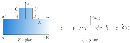
Figure 21: Conformal mapping of the junction between the guide and the side channel.

We note the relationships

$$\frac{\sqrt{1-\sigma^{2}}}{\sigma}=\frac{1}{\theta},\quad\sigma=\frac{\theta}{\sqrt{1+\theta^{2}}}.$$

Harmonic potentials satisfying the homogeneous Neumann condition on the real $\zeta$-axis can be written as a combination of

$$\frac{1}{2\pi}\ln\left(\frac{|\zeta-\sigma|}{2\sigma}\right)\quad\text{and}\quad\frac{1}{2\pi}\ln\left(\frac{|\zeta+\sigma|}{2\sigma}\right),$$ (31)

up to a constant.

We inspect the behaviours of the potentials when $X\to+\infty$ ($|\zeta-\sigma|\sim 0$), $X\to-\infty$ ($|\zeta+\sigma|\sim 0$) in the main channel and when $Y\to+\infty$ ($|\zeta|\to\infty$) in the side channel.

$\bullet$ When $X\to+\infty$, we determine from (30) that

$$\begin{array}[]{l}Z\sim\frac{2}{\pi}\sin^{-1}\sigma+\frac{\sqrt{1-\sigma^{2}}}{\pi\sigma}\ln\left(\frac{2\sigma(1-\sigma^{2})}{-(\zeta-\sigma)}\right),\end{array}$$ (32)

and consequently

$$\begin{array}[]{l}X\sim\frac{2}{\pi}\sin^{-1}\sigma+\frac{\sqrt{1-\sigma^{2}}}{\pi\sigma}\left(\ln(1-\sigma^{2})-\ln\left(\frac{|\zeta-\sigma|}{2\sigma}\right)\right),\end{array}$$ (33)

(which tends to $+\infty$).

$\bullet$ Similarly, as $X\to-\infty$ we have

$$\begin{array}[]{l}X\sim-\frac{2}{\pi}\sin^{-1}\sigma-\frac{\sqrt{1-\sigma^{2}}}{\pi\sigma}\left(\ln(1-\sigma^{2})-\ln\left(\frac{|\zeta+\sigma|}{/2\sigma}\right)\right).\end{array}$$ (34)

$\bullet$ Finally, in the limit $|\zeta|\to+\infty$, we find that

$$\begin{array}[]{l}Z\sim\frac{2\mathrm{i}}{\pi}\ln(-2\mathrm{i}\zeta)+\frac{2\mathrm{i}}{\pi}\frac{\sqrt{1-\sigma^{2}}}{\sigma}\tan^{-1}\left(\frac{\sqrt{1-\sigma^{2}}}{\sigma}\right),\end{array}$$ (35)

meaning that

$$\begin{array}[]{l}Y\sim\frac{2}{\pi}\ln(2|\zeta|)+\frac{2}{\pi}\frac{\sqrt{1-\sigma^{2}}}{\sigma}\tan^{-1}\left(\frac{\sqrt{1-\sigma^{2}}}{\sigma}\right),\end{array}$$ (36)

(which tends to $+\infty$).

We deduce in terms of original variables that

$$\left\{\begin{array}[]{ll}x\to+\infty,&\frac{1}{\pi}\ln\frac{|\zeta-\sigma|}{2\sigma}\sim-\frac{x}{d}-\frac{{\cal A}}{2},\vspace{.2cm}\\ x\to-\infty,&\frac{1}{\pi}\ln\frac{|\zeta+\sigma|}{2\sigma}\sim\frac{x}{d}-\frac{{\cal A}}{2},\vspace{.2cm}\\ y\to+\infty,&\frac{2}{\pi}\ln|2\zeta|\sim\frac{y}{a}+\frac{2}{\pi\theta}\tan^{-1}\theta\end{array}\right.$$ (37)

where ${\cal A}/2=-\frac{2\theta}{\pi}\tan^{-1}\theta+\frac{1}{\pi}\ln(1+\theta^{2})$ (we have used that $\tan^{-1}(1/\theta)+\tan^{-1}\theta=\pi/2$). According to the above behaviour, we recognize $(\psi,\psi_{\text{\tiny s}})$ of the form

$$\psi=\frac{1}{\pi}\ln\frac{|\zeta+\sigma|}{|\zeta-\sigma|},\quad\psi_{\text{\tiny s}}=\frac{1}{\pi}\ln\frac{|\zeta+\sigma||\zeta-\sigma|}{4\sigma^{2}}+\frac{{\cal A}}{2}.$$ (38)

Indeed, we have

$$\begin{array}[]{l}\psi\underset{x\to+\infty}{\sim}-\frac{1}{\pi}\ln\frac{|\zeta-\sigma|}{2\sigma}\sim\frac{x}{d}+\frac{{\cal A}}{2},\vspace{.2cm}\\ \psi\underset{x\to-\infty}{\sim}\frac{1}{\pi}\ln\frac{|\zeta+\sigma|}{2\sigma}\sim\frac{x}{d}-\frac{{\cal A}}{2},\vspace{.2cm}\\ \psi\underset{y\to+\infty}{\sim}0,\end{array}$$ (39)

(as in (6)) which provides ${\cal A}$. We also have

$$\begin{array}[]{l}\psi_{\text{\tiny s}}\underset{x\to+\infty}{\sim}\frac{1}{\pi}\ln\frac{|\zeta-\sigma|}{2\sigma}+\frac{{\cal A}}{2}\sim-\frac{x}{d},\vspace{.2cm}\\ \psi_{\text{\tiny s}}\underset{x\to-\infty}{\sim}\frac{1}{\pi}\ln\frac{|\zeta+\sigma|}{2\sigma}+\frac{{\cal A}}{2}\sim\frac{x}{d},\vspace{.2cm}\\ \psi_{\text{\tiny s}}\underset{y\to+\infty}{\sim}\frac{2}{\pi}\ln\frac{|\zeta|}{2\sigma}+\frac{{\cal A}}{2}\sim\frac{y}{a}+{\cal A}_{\text{\tiny s}},\end{array}$$ (40)

with ${\cal A}_{\text{\tiny s}}=\frac{2}{\pi}\left(\ln\frac{1+\theta^{2}}{4\theta}+(1/\theta-\theta)\tan^{-1}\theta\right)$ (as in (6)) which provides ${\cal A}_{\text{\tiny s}}$.

Appendix B The effective parameters

The variations of $({\cal A},{\cal A}_{\text{\tiny s}})$ for a single channel and of $({\cal B},{\cal B}_{\text{\tiny s}},{\cal B}_{\text{\tiny a}},\hat{\cal B}_{\text{\tiny a}})$ for a pair of channels against $d/2a$ are shown in figure 22; for a pair of the channels, the variations of the effective parameters against $h/2a$ are shown in 23. We note that the parameters $({\cal A},{\cal A}_{\text{\tiny s}})$ and $({\cal B},{\cal B}_{\text{\tiny s}})$ have strong variations when $d/2a<\sim 0.2$ responsible for the shifts of the frequency realizing perfect transmission in figures 14 (shift to higher frequencies for a single channel and shift to a lower frequency for a pair of channels).

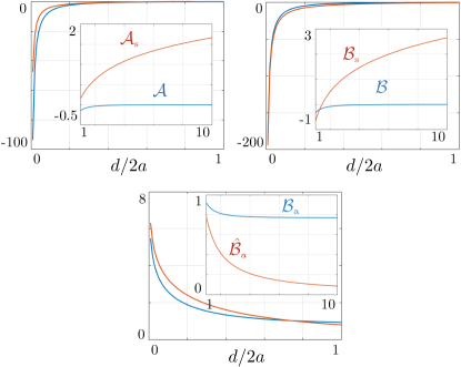
Figure 22: Variations of $({\cal A},{\cal A}_{\text{\tiny s}})$ against $d/2a$ (from (8)), and of $({\cal B},{\cal B}_{\text{\tiny s}},{\cal B}_{\text{\tiny a}},\hat{\cal B}_{\text{\tiny a}})$ (for $h=a$, computed numerically).

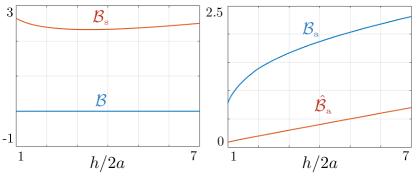
Figure 23: Variations of $({\cal B},{\cal B}_{\text{\tiny s}},{\cal B}_{\text{\tiny a}},\hat{\cal B}_{\text{\tiny a}})$ against $h/2a$ (for $d/2a=10$).

In (26) and (27), we provide an approximate expression of $T$ around $kb=\pi/2$. Orginally, the Taylor expansion provides (25) with

$$k_{0}^{\pm}=\frac{\pi}{2b}\left(1-\frac{a}{2b}\left({\cal B}_{\text{\tiny s}}-{\cal B}+{\cal B}_{\text{\tiny a}}\pm\sqrt{\Delta}\right)\right),$$

with $\Delta=({\cal B}_{\text{\tiny s}}-{\cal B}-{\cal B}_{\text{\tiny a}})^{2}-4\hat{\cal B}_{\text{\tiny a}}^{2}$ and

$$\left\{\begin{array}[]{l}k^{+}=\frac{\pi}{2b}\left(1-\frac{a}{b}{\cal B}_{\text{\tiny a}}-i\frac{\pi ad}{4b^{2}}\hat{\cal B}_{\text{\tiny a}}^{2}\right),\vspace{.2cm}\\ k^{-}=\frac{\pi}{2b}\left(1-\frac{a}{b}{\cal B}_{\text{\tiny s}}\right)-i\frac{2\theta}{b}.\end{array}\right.$$

From figures 22 and for $d/2a>\sim 2$, we notice that ${\cal A}_{\text{\tiny s}}\gg{\cal A}$, hence $k_{0}b\sim\pi/2(1-\frac{a}{b}{\cal A}_{\text{\tiny s}})$. We also notice that ${\cal B}_{\text{\tiny s}}\gg{\cal B}$ and $({\cal B}_{\text{\tiny a}}+{\cal B}_{\text{\tiny s}})\simeq 2{\cal A}_{\text{\tiny s}}$. Hence, defining $2\delta_{r}=({\cal B}_{\text{\tiny s}}-{\cal B}_{\text{\tiny a}})$ (hence ${\cal B}_{\text{\tiny s}}={\cal A}_{\text{\tiny s}}+\delta_{r}$ and ${\cal B}_{\text{\tiny a}}={\cal A}_{\text{\tiny s}}-\delta_{r}$), we obtain the form of $k_{0}^{\pm}$ in (26) and $k^{\pm}$ in (27).

Appendix C Transmission by four channels

We provide in figure 24 additional results on the transmission spectra for different values of $H/2a$ (same representation as in figure 16). The different branches have been identified thanks to the amplitudes in the four channels as in figure 18.

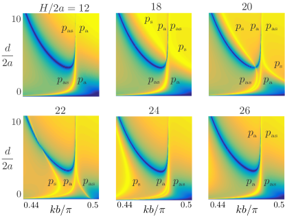
Figure 24: Transmission spectra (in log-scale) against non-dimensional frequency $kb/\pi$ and non-dimensional guide width $d/2a$ for different spacings $H/2a$.

We have already noticed that the central branch corresponds to perfect transmission by each pair of channels which behaves as if it was alone. Accordingly, this branch is almost identical to that reported in figure 14 for a single pair of channels, and we now notice that this remains true whatever the value of $H$. Next, the branches $p_{\text{\tiny a}}$ and $p_{\text{\tiny as}}$ remain close to each other whatever the value of $H$ but their relative positions change (see $H/2a=12$ and 26). This rearrangement is attributable to the interaction of $p_{\text{\tiny as}}$ with the branch $p_{\text{\tiny s}}$ for $H/2a$ between roughly 16 and 21. This later arrives from the high frequency region ($0.5<kh/\pi<1$) and it is shifted to lower frequency as $H$ increases, a trajectory which was already observed for two channels, see figure 8. It is worth noticing that the conversion of $p_{\text{\tiny as}}$ to $p_{\text{\tiny s}}$ on the lower branch correspond to a sudden change in the amplitudes $A_{1}$ and $A_{4}$ when the Fano resonance disappears (see figure 18). In contrast the conversion of $p_{\text{\tiny s}}$ to $p_{\text{\tiny as}}$ on the upper branch does not conduct to the suppression of the associated perfect-transmission. Instead, the amplitudes $A_{1}$ and $A_{4}$ vanish and the Fano resonance is supported by the two central channels only.

References

- Tekman and Bagwell (1993) E. Tekman and P. F. Bagwell, Physical Review B 48, 2553 (1993).
- Kushwaha et al. (1998) M. Kushwaha, A. Akjouj, B. Djafari-Rouhani, L. Dobrzynski, and J. Vasseur, Solid state communications 106, 659 (1998).
- El Boudouti et al. (2008) E. El Boudouti, T. Mrabti, H. Al-Wahsh, B. Djafari-Rouhani, A. Akjouj, and L. Dobrzynski, Journal of Physics: Condensed Matter 20, 255212 (2008).
- Kaina et al. (2013) N. Kaina, M. Fink, and G. Lerosey, Scientific reports 3, 1 (2013).
- Theocharis et al. (2014) G. Theocharis, O. Richoux, V. R. García, A. Merkel, and V. Tournat, New Journal of Physics 16, 093017 (2014).
- Santillán and Bozhevolnyi (2014) A. Santillán and S. I. Bozhevolnyi, Physical Review B 89, 184301 (2014).
- Merkel et al. (2015) A. Merkel, G. Theocharis, O. Richoux, V. Romero-García, and V. Pagneux, Applied Physics Letters 107, 244102 (2015).
- Leclaire et al. (2015) P. Leclaire, O. Umnova, T. Dupont, and R. Panneton, the Journal of the Acoustical Society of America 137, 1772 (2015).
- Anisimov et al. (2011) P. M. Anisimov, J. P. Dowling, and B. C. Sanders, Physical Review Letters 107, 163604 (2011).
- Peng et al. (2014) B. Peng, Ş. K. Özdemir, W. Chen, F. Nori, and L. Yang, Nature communications 5, 1 (2014).
- Jin et al. (2018) Y. Jin, Y. Pennec, and B. Djafari-Rouhani, Journal of Physics D: Applied Physics 51, 494004 (2018).
- Liu et al. (2019) Y. Liu, A. Talbi, O. Bou Matar, P. Pernod, B. Djafari-Rouhani, et al., Physical Review Applied 11, 064066 (2019).
- Cheng et al. (2019) Y. Cheng, Y. Jin, Y. Zhou, T. Hao, and Y. Li, Physical Review Applied 12, 044025 (2019).
- Wang et al. (2021) W. Wang, J. Iglesias, Y. Jin, B. Djafari-Rouhani, and A. Khelif, APL Materials 9, 051125 (2021).
- Wang et al. (2014) Y.-F. Wang, V. Laude, and Y.-S. Wang, Journal of Physics D: Applied Physics 47, 475502 (2014).
- Wang et al. (2018) T.-T. Wang, Y.-F. Wang, Y.-S. Wang, and V. Laude, Applied Physics Letters 113, 231901 (2018).
- Červenka and Bednařík (2018) M. Červenka and M. Bednařík, The Journal of the Acoustical Society of America 144, 2015 (2018).
- Červenka et al. (2019) M. Červenka, M. Bednařík, and J.-P. Groby, The Journal of the Acoustical Society of America 145, 2210 (2019).
- Chesnel and Nazarov (2018) L. Chesnel and S. A. Nazarov, arXiv preprint arXiv:1801.08889 (2018).
- Maurel et al. (2019) A. Maurel, K. Pham, and J.-J. Marigo, Journal of Fluid Mechanics 871, 350 (2019).
- Jan and Porter (2018) A. U. Jan and R. Porter, The Journal of the Acoustical Society of America 144, 3172 (2018).
- Porter (2018) R. Porter, Scattering in a waveguide with narrow side channels (2018).
- Schnitzer and Porter (2022) O. Schnitzer and R. Porter, arXiv preprint arXiv:2201.03554 (2022).