Lifting-based variational multiclass segmentation algorithm: design, convergence analysis, and implementation with applications in medical imaging

Abstract

We propose, analyze and realize a variational multiclass segmentation scheme that partitions a given image into multiple regions exhibiting specific properties. Our method determines multiple functions that encode the segmentation regions by minimizing an energy functional combining information from different channels. Multichannel image data can be obtained by lifting the image into a higher dimensional feature space using specific multichannel filtering or may already be provided by the imaging modality under consideration, such as an RGB image or multimodal medical data. Experimental results show that the proposed method performs well in various scenarios. In particular, promising results are presented for two medical applications involving classification of brain abscess and tumor growth, respectively. As main theoretical contributions, we prove the existence of global minimizers of the proposed energy functional and show its stability and convergence with respect to noisy inputs. In particular, these results also apply to the special case of binary segmentation, and these results are also novel in this particular situation.

[1]organization=Department of Mathematics, University of Innsbruck,country= Austria

[2]organization=VASCage-Research Centre on Vascular Ageing and Stroke, addressline= Innsbruck, country=Austria

[3]organization=MRC Laboratory of Molecular Biology, Cambridge, country=UK

[4]organization=Department of Neuroradiology, Medical University of Innsbruck, country=Austria

1 Introduction

The aim of segmentation is to divide an image defined on some bounded domain $\Omega\subseteq\mathbb{R}^{2}$ into subregions that are homogeneous with regard to certain characteristics, such as intensity, color, or texture. This process plays a fundamental role in various semantic applications such as object recognition, classification, or medical diagnostics. Many successful image segmentation methods are based on variational and active contour models [1, 2, 3], which have in common that they find optimal segmentations by minimizing an objective function, which generally depends on the given image and the features used to identify the different regions to be segmented.

In the simplest case of binary segmentation, the goal is to divide a given image into two regions, one that represents the object to be recognized and the second one that represents background. A particularly popular approach in that regard is the Chan-Vese model [4], that is based on a level-set function $\phi\colon\Omega\to\mathbb{R}$ defining two regions $\{x\in\Omega\mid\phi(x)\leq 0\}$ and $\{x\in\Omega\mid\phi(x)>0\}$. The level-set function $\phi$ is constructed by minimizing a certain energy functional combining regularity of the segmentation region and fitting to the provided input image. The extension to non-binary segmentation (or multiclass segmentation) is challenging due to several reasons. For example, using $m$ level-set functions naturally yields $2^{m}$ separate regions (corresponding to all possible combinations of overlaps of the individual level-sets), which may be different from the desired number of regions to be segmented. Furthermore, in a naive approach, the segmentation function is applied to the unfiltered original intensity image. In practice, however, other characteristics like texture or color may be better suited to separate individual regions; see [5, 6, 7].

In this paper, we present a variational framework for multiclass segmentation based on lifting the image to be segmented into a space of $K$-channel images (feature maps), on which we apply a proposed variational segmentation functional. The individual channels are generated to well separate the $k$-th class from the remaining classes. This can be achieved, for example, by applying multiple filters or by combining information from naturally occurring channels, as in multimodal medical imaging. Even imperfect separation of the different regions by means of the feature maps can be corrected by the actual segmentation process. It should be noted that the generation of vector-valued feature maps prior to actual segmentation is not a new proposal; see e.g. [8, 9, 10] and the references there. However, the specific segmentation functional, the convergence analysis, and the proposed minimization algorithm are new, and are the key contributions of the present work.

1.1 Proposed lifting-based segmentation

Let $\mathbb{F}$ be a space of functions $f\colon\Omega\to\mathcal{M}$ with values in some manifold $\mathcal{M}$. The manifold $\mathcal{M}$ is generic and, for example, can consist of (a subset of) the real numbers $\mathbb{R}$ in the case of gray-value images, be $\mathbb{R}^{d}$ in the case of multimodal imaging, or it can consist of certain tensors such as in diffusion tensor imaging. After feature lifting, the image values will be elements in $\mathbb{R}^{K}$, with $K+1$ denoting the number of distinct classes. Our aim is solving the following task:

Problem 1.1 (Multiclass segmentation).

Based on specific pre-defined characteristics of the image $f\in\mathbb{F}$, construct a partitioning $\Omega=\bigcup_{k=0}^{K}\Sigma_{k}$ of the domain $\Omega$ into $K+1$ disjoint regions (classes). Each of the regions $\Sigma_{1},\dots,\Sigma_{K}$ represents a specific structure or objects in the given image and $\Sigma_{0}$ represents background.

Let $\operatorname*{BV}(\Omega)$ denote the space of all integrable functions $u\colon\Omega\to\mathbb{R}$ with bounded total variation $\lvert u\rvert_{\rm TV}$, write $\boldsymbol{u}=(u_{k})_{k=1}^{K}$ for $K$-tuples of functions in $\operatorname*{BV}(\Omega)$ and consider the admissible set

$$\mathbb{A}\coloneqq\Bigl{\{}\boldsymbol{u}\in\operatorname*{BV}(\Omega)^{K}\mid\boldsymbol{u}\geq 0\wedge\sum_{k=1}^{K}u_{k}\leq 1\Bigr{\}}\,.$$

Here and below $\boldsymbol{u}\geq 0$ means that $u_{k}\geq 0$ for all $k\in\{1,\dots,K\}$. Moreover, let $i_{\mathbb{A}}\colon\operatorname*{BV}(\Omega)^{K}\to[0,\infty]$ denote the associated indicator function taking the value $0$ inside $\mathbb{A}$ and the value $\infty$ outside of $\mathbb{A}$. Throughout we use boldface notation for various kinds of $K$-tuples such as $\boldsymbol{\phi}=(\phi_{k})_{k=1}^{K}\in L^{\infty}(\Omega)^{K}$ or $\boldsymbol{a}=(a_{k})_{k=1}^{K}\in\mathbb{R}^{K}$.

In this work we propose the following three-step segmentation procedure for solving Problem 1.1 and segmenting the image $f\in\mathbb{F}$ into $K+1$ regions.

1. Lifting: Choose $K$ (feature enhancing) transforms $\Phi_{1},\dots,\Phi_{K}\colon\mathbb{F}\to L^{\infty}(\Omega)$ in such a way that the intensity values of the $k$-th feature map $\phi_{k}\coloneqq\Phi_{k}(f)$ allow to well separate region $\Sigma_{k}$ from the remaining part $\Omega\setminus\Sigma_{k}$.

2. Minimization: For given parameter $\lambda>0$, compute a minimizer $(\boldsymbol{u}^{\lambda},\boldsymbol{a}^{\lambda},\boldsymbol{b}^{\lambda})\in\operatorname*{BV}(\Omega)^{K}\times\mathbb{R}^{2K}$ of the energy functional $\mathcal{E}_{\boldsymbol{\phi};\lambda}\colon\operatorname*{BV}(\Omega)^{K}\times\mathbb{R}^{2K}\to[0,\infty]$,

   $$\mathcal{E}_{\boldsymbol{\phi};\lambda}(\boldsymbol{u},\boldsymbol{a},\boldsymbol{b})\coloneqq i_{\mathbb{A}}(\boldsymbol{u})+\lambda\sum_{k=1}^{K}\lvert u_{k}\rvert_{\rm TV}+\sum_{k=1}^{K}\int_{\Omega}(a_{k}-\phi_{k})^{2}u_{k}+(b_{k}-\phi_{k})^{2}(1-u_{k})\,.$$ (1.1)

3. Assignment: For each $k\in\{0,\dots,K\}$ define $\Sigma_{k}$ as the set of all $x\in\Omega$ such that $u^{\lambda}_{k}(x)$ is maximal among the values $u^{\lambda}_{0}(x),\dots,u^{\lambda}_{K}(x)$ where $u_{0}\coloneqq 1-\sum_{k=1}^{K}u_{k}$.

In some applications, the feature channels $\phi_{1},\dots,\phi_{K}$ may already be provided as the input data without the need of additional filtering. For example, in an RGB image, each channel may represent specific regions well characterized by its color. Further examples of this type are found in medical imaging, if for example, one channel corresponds to a computed tomography (CT) image and another channel to magnetic resonance imaging (MRI) data. In this case, bone structures are well revealed on the CT image, and soft tissue well on the MRI data. Notice, however, that we are also interested in cases where channels are extracted via more general transforms $\Phi_{1},\dots,\Phi_{K}$, for example, by exploiting certain expert knowledge and tailoring the segmentation to specific image features.

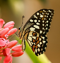
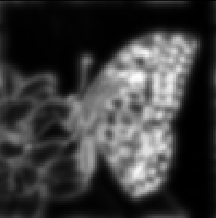
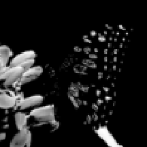
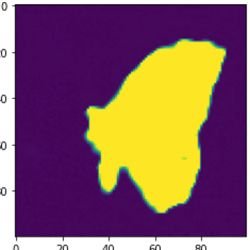
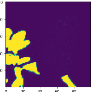
Fig. 1: Illustration of the lifting approach. Top: Given image $f$, computed feature map $\phi_{1}$ (center) targeting the butterfly and feature map $\phi_{2}$ (right) targeting the flower. The lifted version in this case is obtained by color and Gabor filtering. Bottom: resulting minimizers $u_{1}$, $u_{2}$ according to (1.1).

To illustrate the reasoning behind such a strategy, consider the image in the upper left of Fig. 1. The lifted images are obtained by color and Gabor filtering, with parameters provided in Table 1. Suppose we want to identify the butterfly and the flower, and think of the rest as background. Our framework then starts by computing a new set of images (two top right pictures), with the desired structures being highlighted, and then segments those structures via data fitting in the corresponding image channel. Our approach naturally leads to non-overlapping segmentation maps $u_{k}$, for which the constraint $\sum_{k=1}^{K}u_{k}\leq 1$ plays an important role. In particular, by relaxing the condition to $\sum_{k=1}^{K}u_{k}=1$ it implies that no separate channel for the background is required. Segmentation procedure (N1)-(N3) is universal and suitable for any multichannel or multiclass segmentation task.

1.2 Related work

Functional (1.1) is inspired by [11], which introduces a relaxation of the Chan-Vese model for binary segmentation. Actually, for the special case $K=1$, (1.1) reduces to the functional from [11]. One main difference is the soft non-overlapping condition $\sum_{k=1}^{K}u_{k}\leq 1$, which is not required in the binary situation. Moreover, the numerical minimization procedure we propose is very different from the one in [11], which uses an explicit gradient procedure to solve a convex problem with fixed constants, together with occasionally updating constants. In addition, their analysis does not target stability and convergence with respect to the noise level. Extensions of the Chan-Vese model for multiclass segmentation are presented in [12]. In this work, however, $m$ overlapping level-set functions are used, resulting in $2^{m}$ distinct regions to be segmented. The resulting approach is fundamentally different from ours, as optimization is not performed over the segmentation masks $u_{k}$, but rather over the level set functions $\phi_{k}$.

Closely related, yet different approaches that first lift the image into a higher dimensional space of feature maps before applying a segmentation algorithm have also been proposed. In [13, 14], for example, segmentation functionals are used which are independent of the constants $\boldsymbol{a}$ and $\boldsymbol{b}$. This makes the final optimization less general but convex and easier to solve. In our case, due to the presence of unknown constants $\boldsymbol{a}$ and $\boldsymbol{b}$, the functional to be minimized is non-convex and requires the development of efficient algorithms tailored to handle it. In [9], the authors propose a two-step learning approach, in which they learn filters to generate a pre-segmentation in a first step, and apply a modified Mumford-Shah functional in a second step. We develop a numerical algorithm based on a non-convex primal-dual algorithm of [15] for the second step.

Our proposed functional is non-convex because it contains constants $\boldsymbol{a}$ and $\boldsymbol{b}$. Treating these constants as being fixed would result in a convex problem to optimize. It is worth noting that there is also another source of non-convexity in this context, namely, actually working with a Mumford-Shah-like functional instead of using total-variation (TV) to obtain a convex relaxation. This is another challenging yet very exciting direction; see, for example, [16], where an efficient algorithm for solving the Potts model has been developed. Combination and comparison with our multi-channel approach is an interesting line of research, but beyond the scope of this article.

The main contributions of the present paper are threefold. First, we introduce the lifting-based segmentation framework (N1)-(N3) using the energy functional (1.1). Second, we derive a mathematical analysis including stability and convergence with respect to data perturbations. Lastly, we present a numerical algorithm for which we conduct several experiments, in particular for applications in medical imaging. From the mathematical point of view, the most important contributions consist in the presented stability and convergence analysis. To the best of our knowledge, no such results have been previously derived in the literature, not even for the well studied binary segmentation task. Existing theoretical analysis of related models is usually concerned with connections between the relaxed convex minimization problem, (for fixed values $\boldsymbol{a}$, $\boldsymbol{b}$) and the underlying non-convex problem. In contrast, we study both stability and convergence properties of the relaxed functional.

1.3 Outline

The remaining article is structured as follows. In Section 2 we present the mathematical analysis of the proposed multiclass segmentation model (1.1). In Section 3 we develop a numerical algorithm for actual numerical implementation. In Section 4, we present possible applications and experimental results. The paper concludes with a short summary and discussion given in Section 5.

2 Mathematical analysis

We start with the mathematical analysis of the proposed energy functional (1.1). Let $\Omega\subseteq\mathbb{R}^{2}$ be a bounded domain with Lipschitz boundary and denote by $\operatorname*{BV}(\Omega)$ the space of all functions $u\in L^{1}(\Omega)$ with finite (isotropic) total variation

$$\lvert u\rvert_{\rm TV}\coloneqq\lvert\nabla u\rvert_{2,1}\coloneqq\sup\Big{\{}\int_{\Omega}u\operatorname{div}v\mid v\in\mathcal{C}_{c}^{1}(\Omega,\mathbb{R}^{2})\wedge\lvert v\rvert_{2,\infty}\leq 1\Big{\}}\,,$$

where $\lvert v\rvert_{2,\infty}\coloneqq\sup_{x}(v_{1}(x)^{2}+v_{2}(x)^{2})^{1/2}$. Here $\nabla u$ denotes the distributional derivative which for functions $u\in\operatorname*{BV}(\Omega)$ is a vector-valued Radon measure having total mass $\lvert\nabla u\rvert_{2,1}$. It is well known that $\operatorname*{BV}(\Omega)$ with norm $\lVert u\rVert_{\rm TV}\coloneqq\lVert u\rVert_{1}+\lvert u\rvert_{\rm TV}$ is a Banach space.

2.1 Notation and preliminaries

Let $\boldsymbol{\phi}=(\phi_{k})_{k=1}^{K}\in L^{\infty}(\Omega)^{K}$ denote the available multichannel feature map and $\lambda>0$ a regularization parameter. Recall that the channels may either be already provided by the application or may be obtained by application of the feature transforms $\Phi_{k}$; see (N1). Further recall the admissible set $\mathbb{A}$ of (tuples of) segmentation maps, the corresponding indicator function $i_{\mathbb{A}}$ and the functional $\mathcal{E}_{\boldsymbol{\phi};\lambda}$ defined in (1.1). Using the notions

$$\mathcal{D}_{\boldsymbol{\phi}}(\boldsymbol{u},\boldsymbol{a},\boldsymbol{b}) \coloneqq\sum_{k=1}^{K}\int_{\Omega}(a_{k}-\phi_{k})^{2}u_{k}+(b_{k}-\phi_{k})^{2}(1-u_{k})\,,$$

$$\mathcal{Q}(\boldsymbol{u}) \coloneqq\sum_{k=1}^{K}\lvert u_{k}\rvert_{\rm TV}\,,$$

the considered energy functional, for $(\boldsymbol{u},\boldsymbol{a},\boldsymbol{b})\in\operatorname*{BV}(\Omega)^{K}\times\mathbb{R}^{2K}$, takes the form

$$\mathcal{E}_{\boldsymbol{\phi};\lambda}(\boldsymbol{u},\boldsymbol{a},\boldsymbol{b})=i_{\mathbb{A}}(\boldsymbol{u})+\lambda\mathcal{Q}(\boldsymbol{u})+\mathcal{D}_{\boldsymbol{\phi}}(\boldsymbol{u},\boldsymbol{a},\boldsymbol{b})\,.$$ (2.1)

Note that $\operatorname{dom}(\mathcal{E}_{\boldsymbol{\phi};\lambda})\coloneqq\{\boldsymbol{u}\mid\mathcal{E}_{\boldsymbol{\phi};\lambda}(\boldsymbol{u})<\infty\}=\mathbb{A}\times\mathbb{R}^{2K}$ is nonempty, as the segmentation map with constant channels $u_{k}=1/K$ is contained in $\mathbb{A}$. Further, it is worth mentioning that the problem of minimizing (1.1) is bi-convex, meaning it is convex in the variable $\boldsymbol{u}\in\operatorname*{BV}(\mathbb{R})^{K}$ as well as in the variable $(\boldsymbol{a},\boldsymbol{b})\in\mathbb{R}^{2K}$. However it is not jointly convex in both variables. Note that the lower semicontinuity of the total variation (for example, see [17, p. 7]) implies that $\mathcal{Q}(\boldsymbol{u})\leq\liminf_{n\to\infty}\mathcal{Q}(\boldsymbol{u}_{n})$ for any sequence $(\boldsymbol{u}_{n})_{n\in\mathbb{N}}$ with $L^{1}$-limit $\boldsymbol{u}$. Further, at several places of our analysis we make use of the following compactness result.

Lemma 2.1.

If $(\boldsymbol{u}_{n})_{n\in\mathbb{N}}\in(\operatorname*{BV}(\Omega)^{K})^{\mathbb{N}}$ satisfies $i_{\mathbb{A}}(\boldsymbol{u}_{n})+\mathcal{Q}(\boldsymbol{u}_{n})\leq C$ for some constant $C\in(0,\infty)$, then $\lVert\boldsymbol{u}_{\tau(k)}-\boldsymbol{u}\rVert_{1}\to 0$ as $k\to\infty$ for some subsequence $\tau$ and some $\boldsymbol{u}\in\operatorname*{BV}(\Omega)^{K}$.

Proof.

If $i_{\mathbb{A}}(\boldsymbol{u}_{n})+\mathcal{Q}(\boldsymbol{u}_{n})\leq C$, then it holds $0\leq u_{k,n}\leq 1$ and $\lvert u_{k,n}\rvert_{\rm TV}\leq C$ for all $k\in\{1,\dots,K\}$ and $n\in\mathbb{N}$. Therefore the sequences $(\boldsymbol{u}_{k,n})_{n\in\mathbb{N}}$ are bounded in $\operatorname*{BV}(\Omega)$. The compactness theorem for $\operatorname*{BV}(\Omega)$ (see, for example, [18, p. 132] or [19, p. 176]) thus implies the existence of a subsequence $\tau$ and some $\boldsymbol{u}\in\operatorname*{BV}(\Omega)^{K}$ with $\lVert\boldsymbol{u}_{\tau(k)}-\boldsymbol{u}\rVert_{1}\to 0$. ∎

2.2 Reduced formulation

Functional (2.1) is jointly minimized over $\boldsymbol{u}\in\operatorname*{BV}(\Omega)^{K}$ and $(\boldsymbol{a},\boldsymbol{b})\in\mathbb{R}^{2K}$. Throughout this paper we will make use of an equivalent reduced optimization problem in the variable $\boldsymbol{u}$ only, by explicitly computing the minimizers in the variable $(\boldsymbol{a},\boldsymbol{b})$. In that context, we note the following elementary result.

Lemma 2.2.

For all $\boldsymbol{u}\in\mathbb{A}$, the set $\operatorname*{argmin}\mathcal{E}_{\boldsymbol{\phi};\lambda}(\boldsymbol{u},\cdot)$ is non-empty, equals $\operatorname*{argmin}\mathcal{D}_{\boldsymbol{\phi}}(\boldsymbol{u},\cdot)$, and given by

$$\boldsymbol{A}(\boldsymbol{u},\boldsymbol{\phi})\coloneqq\prod_{k=1}^{K}\bigl{(}A(u_{k},\phi_{k}),A(1-u_{k},\phi_{k})\bigr{)}$$ (2.2)

where

$$A(u_{k},\phi_{k}) \coloneqq\begin{cases}\mathbb{R}&\text{ if $u_{k}=0$ }\\ \left\{\frac{1}{\lVert u_{k}\rVert_{1}}\int_{\Omega}\phi_{k}u_{k}\right\}&\text{ otherwise }\,.\end{cases}$$ (2.3)

Proof.

Clearly, $\operatorname*{argmin}\mathcal{E}_{\boldsymbol{\phi};\lambda}(\boldsymbol{u},\cdot)=\operatorname*{argmin}\mathcal{D}_{\boldsymbol{\phi}}(\boldsymbol{u},\cdot)$ and minimizing $\mathcal{D}_{\boldsymbol{\phi}}(\boldsymbol{u},\cdot)$ is separable in the components $a_{k},b_{k}$. Hence minimizers are found by separately minimizing $\int_{\Omega}(a_{k}-\phi_{k})^{2}u_{k}$ with respect to $a_{k}$ and $\int_{\Omega}(b_{k}-\phi_{k})^{2}(1-u_{k})$ with respect to $b_{k}$. We have $\int_{\Omega}(a_{k}-\phi_{k})^{2}u_{k}=a_{k}^{2}\lVert u_{k}\rVert_{1}-2a_{k}\int_{\Omega}\phi_{k}u_{k}+\int_{\Omega}\phi_{k}^{2}u_{k}$ and for $u_{k}\neq 0$ minimizers are given by $\int_{\Omega}\phi_{k}u_{k}/\lVert u_{k}\rVert_{1}$. If $u_{k}=0$ any $a_{k}\in\mathbb{R}$ is a minimizer of $\mathcal{D}_{\boldsymbol{\phi}}(\boldsymbol{u},\cdot)$. Similar arguments for the second minimization problem complete the proof. ∎

Based on Lemma 2.2 we define the reduced energy functional $\mathcal{R}_{\boldsymbol{\phi},\lambda}\colon\operatorname*{BV}(\Omega)^{K}\to[0,\infty]$ by

$$\mathcal{R}_{\boldsymbol{\phi},\lambda}(\boldsymbol{u})\coloneqq\begin{cases}\lambda\mathcal{Q}(\boldsymbol{u})+\inf\mathcal{D}_{\boldsymbol{\phi}}(\boldsymbol{u},\cdot)&\text{ if }\boldsymbol{u}\in\mathbb{A}\,,\\ \infty&\text{ if }\boldsymbol{u}\not\in\mathbb{A}\,.\end{cases}$$ (2.4)

According to Lemma 2.2, the infimum $\inf\mathcal{D}_{\boldsymbol{\phi}}(\boldsymbol{u},\cdot)$ is attained for all $\boldsymbol{u}\in\mathbb{A}$ and the corresponding set of minimizers is given by (2.3). For the following lemma note that $\operatorname*{argmin}\mathcal{R}_{\boldsymbol{\phi},\lambda}\subseteq\mathbb{A}$.

Lemma 2.3 (Equivalence).

For all $(\boldsymbol{u}^{\lambda},\boldsymbol{a}^{\lambda},\boldsymbol{b}^{\lambda})\in\operatorname*{BV}(\Omega)^{K}\times\mathbb{R}^{2K}$ the following statements are equivalent:

1. $(\boldsymbol{u}^{\lambda},\boldsymbol{a}^{\lambda},\boldsymbol{b}^{\lambda})\in\operatorname*{argmin}\mathcal{E}_{\boldsymbol{\phi},\lambda}$.

2. $\boldsymbol{u}^{\lambda}\in\operatorname*{argmin}\mathcal{R}_{\boldsymbol{\phi},\lambda}$ and $(\boldsymbol{a}^{\lambda},\boldsymbol{b}^{\lambda})\in\operatorname*{argmin}\mathcal{D}_{\boldsymbol{\phi}}(\boldsymbol{u}^{{\lambda}},\cdot)$.

Proof.

If $(\boldsymbol{u}^{\lambda},\boldsymbol{a}^{\lambda},\boldsymbol{b}^{\lambda})$ is a minimizer of $\mathcal{E}_{\boldsymbol{\phi},\lambda}$ then clearly $(\boldsymbol{a}^{\lambda},\boldsymbol{b}^{\lambda})\in\operatorname*{argmin}\mathcal{E}_{\boldsymbol{\phi};\lambda}(\boldsymbol{u}^{\lambda},\cdot)$ and for all $\boldsymbol{u}\in\operatorname*{BV}(\Omega)^{K}$ we have $\mathcal{R}_{\boldsymbol{\phi},\lambda}(\boldsymbol{u})\geq\mathcal{E}_{\boldsymbol{\phi},\lambda}(\boldsymbol{u}^{\lambda},\boldsymbol{a}^{\lambda},\boldsymbol{b}^{\lambda})=\mathcal{R}_{\boldsymbol{\phi},\lambda}(\boldsymbol{u}^{\lambda})$. Conversely, if $\boldsymbol{u}^{\lambda}$ minimizes $\mathcal{R}_{\boldsymbol{\phi},\lambda}$ and $(\boldsymbol{a}^{\lambda},\boldsymbol{b}^{\lambda})\in\operatorname*{argmin}\mathcal{E}_{\boldsymbol{\phi};\lambda}(\boldsymbol{u}^{\lambda},\cdot)$, then for $(\boldsymbol{u},\boldsymbol{a},\boldsymbol{b})\in\operatorname*{BV}(\Omega)^{K}\times\mathbb{R}^{2K}$ we have $\mathcal{E}_{\boldsymbol{\phi},\lambda}(\boldsymbol{u},\boldsymbol{a},\boldsymbol{b})\geq\mathcal{R}_{\boldsymbol{\phi},\lambda}(\boldsymbol{u})\geq\mathcal{R}_{\boldsymbol{\phi},\lambda}(\boldsymbol{u}^{\lambda})=\mathcal{E}(\boldsymbol{u}^{\lambda},\boldsymbol{a}^{\lambda},\boldsymbol{b}^{\lambda})$ which completes the proof. ∎

In the following we prove the existence and stability of minimizers of $\mathcal{R}_{\boldsymbol{\phi},\lambda}$ which according to Lemma 2.3 is equivalent to existence and stability of minimizers of $\mathcal{E}_{\boldsymbol{\phi};\lambda}$. We further investigate the convergence of minimizers as the error in the data $\boldsymbol{\phi}$ tends to zero.

2.3 Existence

We start with the existence of minimizers of $\mathcal{R}_{\boldsymbol{\phi},\lambda}$.

Theorem 2.1 (Existence).

For all $\boldsymbol{\phi}\in L^{\infty}(\Omega)^{K}$ and $\lambda>0$, functional $\mathcal{R}_{\boldsymbol{\phi},\lambda}$ admits at least one global minimizer.

Proof.

Since $(1,\dots,1)/K\in\mathbb{A}$, the domain of $\mathcal{R}_{\boldsymbol{\phi},\lambda}$ is non-empty and we can choose a sequence $(\boldsymbol{u}_{n})_{n\in\mathbb{N}}\in\mathbb{A}^{\mathbb{N}}$ such that $\mathcal{R}_{\boldsymbol{\phi},\lambda}(\boldsymbol{u}_{n})\to\inf\mathcal{R}_{\boldsymbol{\phi},\lambda}$. In particular $(i_{\mathbb{A}}(\boldsymbol{u}_{n})+\mathcal{Q}(\boldsymbol{u}_{n}))_{n\in\mathbb{N}}$ is bounded and by Lemma 2.1 there exists a subsequence, again denoted by $(\boldsymbol{u}_{n})_{n\in\mathbb{N}}$, that converges in $L^{1}(\Omega)^{K}$ to some $\boldsymbol{u}^{\lambda}\in L^{\infty}(\Omega)$. By moving to another subsequence, point-wise convergence can be established almost everywhere, from which the conclusion $\boldsymbol{u}^{\lambda}\in\mathbb{A}$ can be drawn. Next, select $(\boldsymbol{a}_{n},\boldsymbol{b}_{n})\in\mathbb{R}^{2K}$ with $\mathcal{R}_{\boldsymbol{\phi},\lambda}(\boldsymbol{u}_{n})=\mathcal{E}_{\boldsymbol{\phi},\lambda}(\boldsymbol{u}_{n},\boldsymbol{a}_{n},\boldsymbol{b}_{n})$ according to (2.2), (2.3). In particular, for $u_{k}\neq 0$ and $u_{k}\neq 1$ we have $a_{k,n}=\lVert u_{k}\rVert_{1}^{-1}\int_{\Omega}\phi_{k}u_{k}$ and $b_{k,n}=\lVert 1-u_{k}\rVert_{1}^{-1}\int_{\Omega}\phi_{k}(1-u_{k})$, respectively. Thus if $\boldsymbol{u}^{\lambda}_{k}\neq 0,1$ for all $k\in\{1,\dots,K\}$ we can assume $u_{k,n}\neq 0,1$ for all $k,n$ and by (2.3) we have

$$0\leq a_{k,n} =\frac{\langle u_{k,n},\phi_{k}\rangle}{\lVert u_{k,n}\rVert_{1}}\leq\lVert\phi_{k}\rVert_{\infty}$$

$$0\leq b_{k,n} =\frac{\langle 1-u_{k,n},\phi_{k}\rangle}{\lVert 1-u_{k,n}\rVert_{1}}\leq\lVert\phi_{k}\rVert_{\infty}\,.$$

If either $u_{k}^{\lambda}=0$ or $u_{k}^{\lambda}=1$, the above identities for $a_{k,n},b_{k,n}$ may not hold. According to Lemma 2.2, in this case the numbers $a_{k,n},b_{k,n}$ can be chosen arbitrarily, and we can therefore still assume that $0\leq a_{k,n},b_{k,n}\leq\lVert\phi_{k}\rVert_{\infty}$. Up to extracting another subsequence, in any case we can assume $(\boldsymbol{a}_{n},\boldsymbol{b}_{n})_{n\in\mathbb{N}}\to(\boldsymbol{a}^{\lambda},\boldsymbol{b}^{\lambda})\in[0,\infty)^{2K}$. Fatou’s Lemma yields

$$\mathcal{D}_{\boldsymbol{\phi}}(\boldsymbol{u}^{\lambda},\boldsymbol{a}^{\lambda},\boldsymbol{b}^{\lambda}) =\sum_{k=1}^{K}\int_{\Omega}(a_{k}^{\lambda}-\phi_{k})^{2}u_{k}^{\lambda}+(b_{k}^{\lambda}-\phi_{k})^{2}(1-u_{k}^{\lambda})$$

$$\leq\sum_{k=1}^{K}\liminf_{n\to\infty}\int_{\Omega}(a_{k,n}-\phi_{k})^{2}u_{k,n}+(b_{k,n}-\phi_{k})^{2}(1-u_{k,n})$$

$$\leq\liminf_{n\to\infty}\mathcal{D}_{\boldsymbol{\phi}}(\boldsymbol{u}_{n},\boldsymbol{a}_{n},\boldsymbol{b}_{n})\,.$$

Together with the lower semi-continuity of $\mathcal{Q}$, we obtain

$$\mathcal{R}_{\boldsymbol{\phi},\lambda}(\boldsymbol{u}^{\lambda}) =i_{\mathbb{A}}(\boldsymbol{u}^{\lambda})+\lambda\mathcal{Q}(\boldsymbol{u}^{\lambda})+\mathcal{D}_{\boldsymbol{\phi}}(\boldsymbol{u}^{\lambda},\boldsymbol{a}^{\lambda},\boldsymbol{b}^{\lambda})$$

$$\leq i_{\mathbb{A}}(\boldsymbol{u}^{\lambda})+\lambda\liminf_{n\to\infty}\mathcal{Q}(\boldsymbol{u}_{n})+\liminf_{n\to\infty}\mathcal{D}_{\boldsymbol{\phi}}(\boldsymbol{u}_{n},\boldsymbol{a}_{n},\boldsymbol{b}_{n})$$

$$\leq\liminf_{n\to\infty}i_{\mathbb{A}}(\boldsymbol{u}_{n})+\lambda\mathcal{Q}(\boldsymbol{u}_{n})+\mathcal{D}_{\boldsymbol{\phi}}(\boldsymbol{u}_{n},\boldsymbol{a}_{n},\boldsymbol{b}_{n})$$

$$\leq\lim_{n\to\infty}i_{\mathbb{A}}(\boldsymbol{u}_{n})+\lambda\mathcal{Q}(\boldsymbol{u}_{n})+\inf_{\boldsymbol{a},\boldsymbol{b}}\mathcal{D}_{\boldsymbol{\phi}}(\boldsymbol{u}_{n},\boldsymbol{a},\boldsymbol{b})$$

$$=\inf\mathcal{R}_{\boldsymbol{\phi},\lambda}$$

Hence $\boldsymbol{u}^{\lambda}$ is a minimizer of $\mathcal{R}_{\boldsymbol{\phi},\lambda}$. ∎

2.4 Stability

Next we investigate the stability of minimizers of $\mathcal{R}_{\boldsymbol{\phi},\lambda}$ with respect to data $\boldsymbol{\phi}$.

Theorem 2.2 (Stability).

Let $\boldsymbol{\phi},\boldsymbol{\phi}_{n}\in L^{\infty}(\Omega)^{K}$ for $n\in\mathbb{N}$ such that $\lVert\boldsymbol{\phi}_{n}-\boldsymbol{\phi}\rVert_{\infty}\to 0$ and take $\boldsymbol{u}_{n}\in\operatorname*{argmin}\mathcal{R}_{\phi_{n},\lambda}$. Then $(\boldsymbol{u}_{n})_{n\in\mathbb{N}}$ has at least one $L^{1}$-norm convergent subsequence and the limit of any $L^{1}$-norm convergent subsequence $(\boldsymbol{u}_{\tau(n)})_{n\in\mathbb{N}}$ is a minimizer $\boldsymbol{u}^{\lambda}$ of $\mathcal{R}_{\boldsymbol{\phi},\lambda}$ that satisfies $\mathcal{Q}(\boldsymbol{u}_{\tau(n)})\to\mathcal{Q}(\boldsymbol{u}^{\lambda})$ as $n\to\infty$.

Proof.

Because $\boldsymbol{u}_{n}\in\operatorname*{argmin}\mathcal{R}_{\phi_{n},\lambda}$, we have that $(\mathcal{R}_{\boldsymbol{\phi}_{n},\lambda}(\boldsymbol{u}_{n}))_{n\in\mathbb{N}}$ is bounded and therefore $(\mathcal{Q}(\boldsymbol{u}_{n}))_{n\in\mathbb{N}}$ is bounded, too. By Theorem 2.1 there exists a subsequence, that we again denote by $(\boldsymbol{u}_{n})_{n\in\mathbb{N}}$, that converges in $L^{1}(\Omega)^{K}$ to some $\boldsymbol{u}^{\lambda}\in\operatorname*{BV}(\Omega)^{K}$. Like in the proof of Theorem 2.1, we construct $(\boldsymbol{a}_{n},\boldsymbol{b}_{n})$ such that $(\boldsymbol{u}_{n},\boldsymbol{a}_{n},\boldsymbol{b}_{n})\in\operatorname*{argmin}\mathcal{E}_{\boldsymbol{\phi}_{n},\lambda}$ and $0\leq a_{k,n},b_{k,n}\leq\lVert\phi_{k,n}\rVert_{\infty}$. As $\lVert\boldsymbol{\phi}_{n}-\boldsymbol{\phi}\rVert_{\infty}\to 0$, the elements $\boldsymbol{\phi}_{n}$ are uniformly bounded and thus $(a_{k,n})_{n\in\mathbb{N}}$ and $(b_{k,n})_{n\in\mathbb{N}}$ are bounded. Therefore, up to the extraction of another subsequence, we can assume $(\boldsymbol{a}_{n},\boldsymbol{b}_{n})\to(\boldsymbol{a}^{\lambda},\boldsymbol{b}^{\lambda})$.

It remains to show that $\boldsymbol{u}^{\lambda}$ is a minimizer of $\mathcal{E}_{\boldsymbol{\phi};\lambda}$ and that $\mathcal{Q}(\boldsymbol{u}_{n})\to\mathcal{Q}(\boldsymbol{u}^{\lambda})$. After passing to a subsequence that converges pointwise almost everywhere, from Fatou’s lemma and the semi-continuity of $\mathcal{Q}$ one derives $\mathcal{R}_{\boldsymbol{\phi},\lambda}(\boldsymbol{u}^{\lambda})\leq\liminf_{n\to\infty}\mathcal{E}_{\boldsymbol{\phi}_{n},\lambda}(\boldsymbol{u}_{n},\boldsymbol{a}_{n},\boldsymbol{b}_{n})$. Therefore, for all $(\boldsymbol{u},\boldsymbol{a},\boldsymbol{b})\in\operatorname*{BV}(\Omega)^{K}\times\mathbb{R}^{2K}$, we have

$$\mathcal{R}_{\boldsymbol{\phi},\lambda}(\boldsymbol{u}^{\lambda}) \leq\liminf_{n\to\infty}i_{\mathbb{A}}(\boldsymbol{u}_{n})+\lambda\mathcal{Q}(\boldsymbol{u}_{n})+\mathcal{D}_{\phi_{n}}(\boldsymbol{u}_{n},\boldsymbol{a}_{n},\boldsymbol{b}_{n})$$

$$\leq\limsup_{n\to\infty}i_{\mathbb{A}}(\boldsymbol{u}_{n})+\lambda\mathcal{Q}(\boldsymbol{u}_{n})+\mathcal{D}_{\phi_{n}}(\boldsymbol{u}_{n},\boldsymbol{a}_{n},\boldsymbol{b}_{n})$$

$$\leq\lim_{n\to\infty}i_{\mathbb{A}}(\boldsymbol{u})+\lambda\mathcal{Q}(\boldsymbol{u})+\mathcal{D}_{\phi_{n}}(\boldsymbol{u},\boldsymbol{a},\boldsymbol{b})$$

$$=i_{\mathbb{A}}(\boldsymbol{u})+\lambda\mathcal{Q}(\boldsymbol{u})+\mathcal{D}_{\phi}(\boldsymbol{u},\boldsymbol{a},\boldsymbol{b})=\mathcal{E}_{\boldsymbol{\phi},\lambda}(\boldsymbol{u},\boldsymbol{a},\boldsymbol{b})\,.$$

Taking the infimum over $(\boldsymbol{a},\boldsymbol{b})$ shows $\mathcal{R}_{\boldsymbol{\phi},\lambda}(\boldsymbol{u}^{\lambda})\leq\mathcal{R}_{\boldsymbol{\phi},\lambda}(\boldsymbol{u})$ which implies $\boldsymbol{u}^{\lambda}\in\operatorname*{argmin}\mathcal{R}_{\boldsymbol{\phi},\lambda}$. Choosing $\boldsymbol{u}=\boldsymbol{u}^{\lambda}$ in the last displayed equation shows $\mathcal{R}_{\boldsymbol{\phi},\lambda}(\boldsymbol{u}^{\lambda})=\lim_{n\to\infty}\lambda\mathcal{Q}(\boldsymbol{u}_{n})+\mathcal{D}_{\phi_{n}}(\boldsymbol{u}_{n},\boldsymbol{a}_{n},\boldsymbol{b}_{n})$ and

$$\limsup_{n\to\infty}\lambda\mathcal{Q}(\boldsymbol{u}_{n})\leq\lim_{n\to\infty}\lambda\mathcal{Q}(\boldsymbol{u}_{n})+\mathcal{D}_{\phi_{n}}(\boldsymbol{u}_{n},\boldsymbol{a}_{n},\boldsymbol{b}_{n})-\liminf_{n\to\infty}\mathcal{D}_{\phi_{n}}(\boldsymbol{u}_{n},\boldsymbol{a}_{n},\boldsymbol{b}_{n})\\ \leq\mathcal{R}_{\boldsymbol{\phi},\lambda}(\boldsymbol{u}^{\lambda})-\mathcal{D}_{\boldsymbol{\phi}}(\boldsymbol{u}^{\lambda},\boldsymbol{a}^{\lambda},\boldsymbol{a}^{\lambda})=\lambda\mathcal{Q}(\boldsymbol{u}^{\lambda})\,,$$

which concludes the proof. ∎

2.5 Convergence

In the following we investigate the convergence of minimizers of $\mathcal{R}_{\boldsymbol{\phi},\lambda}$ to minimizers of the following limiting constraint optimization problem

$$\left\{\begin{aligned} &\min_{\boldsymbol{u}}\mathcal{Q}(\boldsymbol{u})\\ &\text{ s.t. }\boldsymbol{u}\in\operatorname*{argmin}i_{\mathbb{A}}+\inf_{\boldsymbol{a},\boldsymbol{b}}\mathcal{D}_{\boldsymbol{\phi}}(\cdot,\boldsymbol{a},\boldsymbol{b})\,.\end{aligned}\right.$$ (2.5)

In general, $\operatorname*{argmin}i_{\mathbb{A}}+\inf_{\boldsymbol{a},\boldsymbol{b}}\mathcal{D}_{{{\phi}}}(\cdot,\boldsymbol{a},\boldsymbol{b})$ can be empty, reflecting the ill-posedness of (2.5) and the need for the relaxed problem (2.1). However, for certain $\boldsymbol{\phi}$, which we refer to exact data, such minimizers exist and define a segmentation function that is independent of any parameters. When minimizing the energy functional $\mathcal{R}_{\boldsymbol{\phi},\lambda}$, we then interpret $\boldsymbol{\phi}$ as perturbed version of the exact data, and $\lambda$ as regularization parameter accounting for stability. In the convergence analysis, we study convergence of minimizers of $\mathcal{R}_{\boldsymbol{\phi},\lambda}$ to solutions of (2.5) as the noise level and the regularization parameter tend to zero. We are not aware of any such an analysis in the segmentation literature, but think that this approach can be the starting point of new insights and algorithms.

Remark 2.1.

Denote by $\mathbbm{1}_{\Sigma}$ the indicator function of a set $\Sigma\subseteq\Omega$ taking the value $1$ inside $\Sigma$ and $0$ outside. In order to focus on the main ideas, in the following we consider exact feature maps $\boldsymbol{\phi}^{*}\in L^{\infty}(\Omega)^{K}$ with binary channels

$$\phi_{k}^{*}=a_{k}^{*}\mathbbm{1}_{\Sigma_{k}}+b_{k}^{*}\mathbbm{1}_{\Omega\setminus\Sigma_{k}}\,,$$ (2.6)

where

• $\Sigma_{k}\subseteq\Omega$ are pairwise disjoint with finite perimeters

• $(\boldsymbol{a}^{*},\boldsymbol{b}^{*})\in\mathbb{R}^{2K}$ satisfies $\forall k\colon a_{k}^{*}\neq b_{k}^{*}$.

Recall that the perimeter $\operatorname{per}(\Sigma)\coloneqq\lvert\mathbbm{1}_{\Sigma}\rvert_{\rm TV}$ of a set $\Sigma$ is defined as the total variation of the indicator function $\mathbbm{1}_{\Sigma}$. In particular, functions of the form (2.6) satisfy $\lvert\phi_{k}\rvert_{\rm TV}=\lvert b_{k}^{*}-a_{k}^{*}\rvert\operatorname{per}(\Sigma_{k})$.

Lemma 2.4.

For any exact data $\boldsymbol{\phi}^{*}\in L^{\infty}(\Omega)^{K}$ of the form (2.6), the set of solutions of (2.5) is non-empty and consists of all $\boldsymbol{u}^{\star}\in\operatorname*{BV}(\Omega)^{K}$ with $u_{k}^{\star}\in\{\mathbbm{1}_{\Sigma_{k}},\mathbbm{1}_{\Omega\setminus\Sigma_{k}}\}$.

Proof.

Let $u_{k}^{\star}\in\{\mathbbm{1}_{\Sigma_{k}},\mathbbm{1}_{\Omega\setminus\Sigma_{k}}\}$. Clearly, $0\leq\mathcal{R}_{\boldsymbol{\phi}^{*},0}$ and $0=\mathcal{R}_{\boldsymbol{\phi}^{*},0}(\boldsymbol{u}^{\star})$. Therefore $\boldsymbol{u}^{\star}\in\operatorname*{argmin}i_{\mathbb{A}}+\inf_{\boldsymbol{a},\boldsymbol{b}}\mathcal{D}_{\boldsymbol{\phi}}(\cdot,\boldsymbol{a},\boldsymbol{b})$. Moreover, $\mathcal{Q}(\boldsymbol{u}^{\star})=\sum_{k=1}^{K}\operatorname{per}(\Sigma_{k})$ which shows that $\boldsymbol{u}^{*}$ solves (2.5). ∎

We now have the following convergence result.

Theorem 2.3 (Convergence).

Let $\boldsymbol{\phi}^{*}\in L^{\infty}(\Omega)^{K}$ be exact data of the form (2.6), $(\delta_{n})_{n\in\mathbb{N}}\in(0,\infty)^{\mathbb{N}}$ converge to zero and $(\boldsymbol{\phi}_{n})_{n\in\mathbb{N}}\in L^{\infty}(\Omega)^{K}$ be noisy data with $\lVert\boldsymbol{\phi}^{*}-\boldsymbol{\phi}_{n}\rVert_{\infty}\leq\delta_{n}$. Further, let $\lambda_{n}\in(0,\infty)^{\mathbb{N}}$ be a sequence of regularization parameters with $\lambda_{n}\to 0$ and $\delta_{n}^{2}/\lambda_{n}\to 0$ and let $\boldsymbol{u}_{n}\in\operatorname*{argmin}\mathcal{R}_{\boldsymbol{\phi}_{n},\lambda_{n}}$. Then $(\boldsymbol{u}_{n})_{n\in\mathbb{N}}$ has at least one $L^{1}$-convergent subsequence. Moreover, the limit of any $L^{1}$-convergent subsequence $(\boldsymbol{u}_{\tau(n)})_{n\in\mathbb{N}}$ is a solution $\boldsymbol{u}^{*}$ of (2.5) with $\mathcal{Q}(\boldsymbol{u}_{\tau(n)})\to\mathcal{Q}(\boldsymbol{u}^{*})$.

Proof.

According to Lemma 2.4, $\boldsymbol{u}^{*}=(\mathbbm{1}_{\Sigma_{k}})_{k\in\mathbb{N}}$ is a solution of (2.5). Further, we have

$$\mathcal{D}_{\boldsymbol{\phi}_{n}}(\boldsymbol{u}^{*},\boldsymbol{a}^{*},\boldsymbol{b}^{*})=\sum_{k=1}^{K}\int_{\Sigma_{k}}{(\phi_{k,n}-a_{k}^{*})^{2}}+\int_{\Omega\setminus\Sigma_{k}}(\phi_{k,n}-b_{k}^{*})^{2}=\sum_{k=1}^{K}\int_{\Omega}(\phi_{k,n}-\phi_{k}^{*})^{2}\leq K\lvert\Omega\rvert\delta_{n}^{2}\,.$$

Together with the definition of $\boldsymbol{u}_{n}$ and choosing elements $(\boldsymbol{a}_{n},\boldsymbol{b}_{n})\in\operatorname*{argmin}\mathcal{D}_{\phi_{n}}(\boldsymbol{u}_{n},\cdot)$ this shows

$$\mathcal{D}_{\phi_{n}}(\boldsymbol{u}_{n},\boldsymbol{a}_{n},\boldsymbol{b}_{n})+\lambda_{n}\mathcal{Q}(\boldsymbol{u}_{n})\leq K\lvert\Omega\rvert\delta_{n}^{2}+\lambda_{n}\mathcal{Q}(\boldsymbol{u}^{*})\,.$$

Together with the parameter choice $\lambda_{n},\delta_{n}^{2}/\lambda_{n}\to 0$ and the continuity of $\mathcal{D}_{\boldsymbol{\phi}_{n}}(\boldsymbol{u}_{n},\boldsymbol{a}_{n},\boldsymbol{b}_{n})$ in $\boldsymbol{\phi}_{n}$ this shows

$$\lim_{n\to\infty}\mathcal{D}_{\boldsymbol{\phi}_{n}}(\boldsymbol{u}_{n},\boldsymbol{a}_{n},\boldsymbol{b}_{n})=0$$ (2.7)

$$\limsup_{n\to\infty}\mathcal{Q}(\boldsymbol{u}_{n})\leq\mathcal{Q}(\boldsymbol{u}^{*})\,.$$ (2.8)

Lemma 2.1 and identity (2.8) imply the existence of an $L^{1}$-convergent subsequence $(\boldsymbol{u}_{\tau(n)})_{n\in\mathbb{N}}$. According to (2.7), the limit of any such subsequence is a solution of (2.5) and without loss of generality we can assume $\boldsymbol{u}_{\tau(n)}\to\boldsymbol{u}^{*}$. From (2.8) and the lower semi-continuity of $\mathcal{Q}$ we finally derive $\mathcal{Q}(\boldsymbol{u}_{\tau(n)})\to\mathcal{Q}(\boldsymbol{u}^{*})$. ∎

3 Algorithm development

In this section, we establish a numerical algorithm for minimizing the reduced segmentation functional $\mathcal{R}_{f,\lambda}$. For that purpose, we will first introduce a discrete framework for which we actually present our optimization procedure.

3.1 Discretization

In the following we work with discrete images and feature maps in $\mathbb{H}\coloneqq\mathbb{R}^{N_{1}\times N_{2}}$, which is a finite dimensional Hilbert space with inner product $\langle u,v\rangle=\sum_{i}u[i]v[i]$ for $u,v\in\mathbb{H}$ where $i=(i_{1},i_{2})\in\{1,\dots,N_{1}\}\times\{1,\dots,N_{2}\}$. Moreover we introduce the following discrete counterparts of ingredients of the continuous functional (2.4).

• The discrete gradient $\nabla=(\nabla_{1},\nabla_{2})\colon\mathbb{H}\to\mathbb{H}\times\mathbb{H}$ is defined by forward differences with Neumann boundary conditions

  $$(\nabla_{1}u)[i] \coloneqq\begin{cases}(u[i_{1}+1,i_{2}]-u[i_{1},i_{2}])/h&\text{if }i_{1}<N_{1}\\ 0&\text{if }i_{1}=N_{1}\end{cases}$$

  $$(\nabla_{2}u)[i] \coloneqq\begin{cases}(u[i_{1},i_{2}+1]-u[i_{1},i_{2}])/h&\text{if }i_{2}<N_{2}\\ 0&\text{if }i_{2}=N_{2}\,.\end{cases}$$

  Its adjoint is given by $\nabla^{*}(v_{1},v_{2})=\nabla^{*}_{1}v_{1}+\nabla_{2}^{*}v_{2}=:-\operatorname{div}(v_{1},v_{2})$ where $\operatorname{div}\colon\mathbb{H}\times\mathbb{H}\to\mathbb{H}$ is the discrete divergence operator and for $(v_{1},v_{2})\in\mathbb{H}\times\mathbb{H}$ we have

  $$(\nabla^{*}_{1}v_{1})[i] =\begin{cases}-(v_{1}[i_{1},i_{2}]-v_{1}[i_{1}-1,i_{2}])/h&\text{if }1<i_{1}<N_{1}\\ -v_{1}[1,i_{2}]&\text{if }i_{1}=1\\ \phantom{-}v_{1}[N_{1}-1,i_{2}]&\text{if }i_{1}=N_{1}\end{cases}$$

  $$(\nabla^{*}_{2}v_{2})[i] =\begin{cases}-(v_{2}[i_{1},i_{2}]-v_{2}[i_{1},i_{2}-1])/h&\text{if }1<i_{2}<N_{2}\\ -v_{2}[i_{1},1]&\text{if }i_{2}=1\\ \phantom{-}v_{2}[i_{1},N_{2}-1]&\text{if }i_{2}=N_{2}\,.\end{cases}$$

  Finally we write $\boldsymbol{\nabla}\boldsymbol{u}\coloneqq(\nabla u_{1},\dots,\nabla u_{K})$ for the discrete gradient applied componentwise to $\boldsymbol{u}\in\mathbb{H}^{K}$.

• The discrete (isotropic) TV semi-norm of some image $u\in\mathbb{H}$ is defined as

  $$\lVert\nabla_{1}u\rVert_{1,2}\coloneqq\sum_{i}\sqrt{(\nabla_{1}u[i])^{2}+(\nabla_{2}u[i])^{2}}\,.$$

  We write $\mathbb{A}=\{\boldsymbol{u}\in\mathbb{H}^{K}\mid\boldsymbol{u}\geq 0\wedge\sum_{k}u_{k}=1\}$ for the discrete admissible set and $i_{\mathbb{A}}$ for the corresponding indicator function.

• Let $\mathbbm{1}\in\mathbb{H}$ denotes the all-ones image, $\boldsymbol{\phi}=(\phi_{k})_{k=1}^{K}\in\mathbb{H}^{K}$ the discrete feature map with $K$-channels to be segmented and $\boldsymbol{u}=(u_{k})_{k=1}^{K}\in\mathbb{H}^{K}$ the desired segmentation function. The discretization of the data fitting term in the reduced energy is written as $\lVert\boldsymbol{M}(\boldsymbol{u})\rVert_{1}$ where

  $$\boldsymbol{M}(\boldsymbol{u})\coloneqq(m(u_{k}),m(1-u_{k}))_{k=1}^{K}$$ (3.1)

  $$m(u_{k})\coloneqq u_{k}\cdot(A(u_{k})\mathbbm{1}-\phi_{k})^{2}$$ (3.2)

  $$A(u)\coloneqq\langle u_{k},\phi_{k}\rangle/\lvert u_{k}\rvert_{1,\epsilon}\,.$$ (3.3)

  Here $\lVert\cdot\rVert_{1}$ is the $\ell_{1}$-norm applied to $\boldsymbol{M}(\boldsymbol{u})\in\mathbb{H}^{2K}$ and the averages $A(\cdot)$ use the approximation $\lvert u\rvert_{1,\epsilon}\coloneqq\sum_{i}(u[i]^{2}+\epsilon)^{1/2}$ of the $\ell_{1}$-norm, making it single-valued and twice differentiable.

Using the notions given above, the discrete reduced energy functional reads

$$\mathcal{R}_{\boldsymbol{\phi},\lambda}(\boldsymbol{u})\coloneqq i_{\mathbb{A}}(\boldsymbol{u})+\lambda\sum_{k=1}^{K}\lVert\nabla u_{k}\rVert_{1,2}+\lVert\boldsymbol{M}(\boldsymbol{u})\rVert_{1,1}\,.$$ (3.4)

Optimization problem (3.4) is a non-convex, non-smooth and a challenging large scale problem to be solved. Its particular structure, however, allows to apply various splitting type optimization algorithms. In particular, we will demonstrate that it can be solved with the algorithm of [15], which itself is a generalization of the Chambolle-Pock algorithm [20] for convex problems.

3.2 Nonlinear primal dual algorithm

Our algorithm is a particular instance of the primal dual hybrid gradient (PDHG) algorithm of [15], which is a generic algorithmic framework solving minimization problems of the following composite form

$$\min_{x\in\mathbb{X}}\mathcal{F}(K(x))+\mathcal{G}(x)\,,$$ (3.5)

where $K\colon\mathbb{X}\to\mathbb{Y}$ is a possibly nonlinear mapping between Hilbert spaces $\mathbb{X}$, $\mathbb{Y}$ and $\mathcal{F}\colon\mathbb{Y}\to[0,\infty]$ and $\mathcal{G}\colon\mathbb{X}\to[0,\infty]$ are convex and lower semi-continuous functionals. Essential components of the PDHG algorithm are the proximal operator $\operatorname{prox}_{\mathcal{H}}\colon\mathbb{X}\to\mathbb{X}$ and the Fenchel conjugate $\mathcal{H}^{*}\colon\mathbb{X}\to[0,\infty]$, respectively, associated to a given functional $\mathcal{H}\colon\mathbb{X}\to[0,\infty]$, defined by

$$\operatorname{prox}_{\mathcal{H}}(x) =\operatorname*{argmin}_{z\in\mathbb{X}}\mathcal{H}(z)+\frac{1}{2}\lVert z-x\rVert^{2}$$

$$\mathcal{H}^{*}(x) =\sup_{z\in\mathbb{X}}\langle x,z\rangle-\mathcal{H}(z)\,.$$

Note that the nonlinear PDHG algorithm itself is an extension of primal dual optimization scheme proposed in [20] from linear to nonlinear operators.

The PDHG algorithm for (3.5) with parameters $\sigma,\tau>0$ and $\theta\in[0,1]$ generates a sequence $(x^{n},\bar{x}^{n},y^{n})_{n\in\mathbb{N}}\in(\mathbb{X}\times\mathbb{X}\times\mathbb{Y})^{\mathbb{N}}$ by

$$y^{n+1} \coloneqq\operatorname{prox}_{\sigma\mathcal{F}^{*}}(y^{n}+\sigma K(\bar{x}^{n}))$$ (3.6)

$$x^{n+1} \coloneqq\operatorname{prox}_{\tau\mathcal{G}}(x^{n}-\tau K^{\prime}(x^{n})^{*}y^{n})$$ (3.7)

$$\bar{x}^{n+1} \coloneqq x^{n+1}+\theta(x^{n+1}-x^{n})\,,$$ (3.8)

for some initializations $x^{0},\bar{x}^{0}\in\mathbb{X}$ and $y^{0}\in\mathbb{Y}$. Here $K^{\prime}(x)^{*}$ is the adjoint of the derivative of $K$ at $x$. Convergence of (3.6)-(3.8) to saddle points of (3.5) has been analyzed in [15].

3.3 Derivation of algorithm

Inspecting the functional (3.4) to be minimized and the PDHG algorithm (3.6)-(3.8) for the generic problem (3.5), we see that it can be applied to our setting with

$$\mathbb{X} =\mathbb{H}^{K}$$

$$\mathbb{Y} =\mathbb{H}^{2K}\times\mathbb{H}^{2K}$$

$$K =(\boldsymbol{\nabla},\boldsymbol{M})$$

$$\mathcal{F}(\boldsymbol{v},\boldsymbol{w}) =\lambda\lVert\boldsymbol{v}\rVert_{2,1}+\lVert\boldsymbol{w}\rVert_{1,1}$$

$$\mathcal{G} =i_{\mathbb{A}}\,.$$

Recall that $\boldsymbol{M}$ defined by (3.1)-(3.3) is nonlinear and therefore $K$ is nonlinear, too. Further, the functionals $\mathcal{F}$ and $\mathcal{G}$ are convex and lower semi-continuous. The actual practical implementation requires computing proximal mappings, derivatives, and Fenchel conjugates. This will be done in the following.

• Fenchel conjugate of $\mathcal{F}$: The functional $\mathcal{F}$ is separable in $\boldsymbol{v}$ and $\boldsymbol{w}$, and therefore its Fenchel conjugate is a sum of the Fenchel conjugates of $\lVert\cdot\rVert_{2,1}$ and $\lVert\cdot\rVert_{1,1}$, which are both well known. Actually, they are given by indicator functions of the unit ball of the dual norms and therefore

  $$\mathcal{F}^{*}(\boldsymbol{v},\boldsymbol{w})=i_{2,\infty}(\boldsymbol{v}/\lambda)+i_{\infty,\infty}(\boldsymbol{w})\,.$$

  Here $i_{q,\infty}=\lVert\cdot\rVert_{q,\infty}^{*}$ denotes the indicator function of the unit ball $\{\boldsymbol{v}\mid\lVert\boldsymbol{v}\rVert_{q,\infty}\leq 1\}\subseteq(\mathbb{H}^{K})^{2}$ for the norm $\lVert\cdot\rVert_{q,\infty}$ for $q=2,\infty$.

• Proximal operators of $\mathcal{F}^{*}$, $\mathcal{G}$: Let us next compute the proximal operator of $\mathcal{F}^{*}(\boldsymbol{v},\boldsymbol{w})=i_{2,\infty}(\boldsymbol{v}/\lambda)+i_{\infty,\infty}(\boldsymbol{w})$ which is the separable sum of two indicator functions. The proximal operator of the indicator function $i_{S}$ of some set $S$ is known to be given as the projection on $S$. The projections $P_{\infty,p}\colon(\mathbb{H}^{K})^{2}\to(\mathbb{H}^{K})^{2}$ onto the unit ball in the $(\infty,q)$-norm for $q=2,\infty$ can easily be computed and given by

  $$(P_{2,\infty}(\boldsymbol{v}))[i,k]=\frac{v[i,k]}{\max\{1,(v_{1}[i,k]^{2}+v_{2}[i,k])^{1/2}\}}$$

  $$(P_{\infty,\infty}(p))[i,k]=\Bigl{(}\frac{v_{j}[i,k]}{\max\{1,v_{j}[i,k]\}}\Bigr{)}_{j=1,2}\,.$$

  Thus the proximal operator of $\mathcal{F}^{*}$ is given by

  $$\operatorname{prox}_{\mathcal{F}^{*}}(\boldsymbol{v},\boldsymbol{w})=(P_{2,\infty}(\boldsymbol{v}/\lambda),P_{\infty,\infty}(\boldsymbol{w}))\,.$$

  The proximal operator of $\mathcal{G}=i_{\mathbb{A}}$ is the orthogonal projection $P_{\mathbb{A}}$ onto the simplex $\mathbb{A}$. In this case, no explicit formula is available. However, the projection can be computed with a finite number of steps, and for our implementation we use the algorithm proposed in [21] for that purpose.

• Derivative computation: Finally we compute the adjoint of the derivative of $K=(\boldsymbol{\nabla},\boldsymbol{M})$. The discrete gradient operator is linear and therefore $\boldsymbol{\nabla}^{\prime}(\boldsymbol{u})=\boldsymbol{\nabla}$. Further from (3.1)-(3.3) we see that computing the derivative of $K$ amounts to computing the derivative of

  $$m(u)=u\cdot\left(\frac{\langle u,\phi\rangle}{\lvert u\rvert_{1,\epsilon}}\mathbbm{1}-\phi\right)^{2}\,.$$

  For that purpose we write $\phi,u\in\mathbb{H}$ as column vectors,

  $$u =(u_{1},\dots,u_{N})^{\intercal}\in\mathbb{R}^{N}$$

  $$\phi =(\phi_{1},\dots,\phi_{N})^{\intercal}\in\mathbb{R}^{N}$$

  with $N\coloneqq N_{1},N_{2}$. By the chain rule we find that the derivative $(Dm)(u)$ and its adjoint are given by the following $N\times N$ matrices

  $$(Dm)(u) =T(u)^{2}-2U(u)T(u)Q(u)$$ (3.9)

  $$(Dm)(u)^{*} =T(u)^{2}-2Q(u)^{\intercal}T(u)U(u)$$ (3.10)

  where

  $$T(u) \coloneqq\operatorname{diag}\bigl{(}\langle u,\phi\rangle\lvert u\rvert_{1,\epsilon}^{-1}\mathbbm{1}-\phi\bigr{)}$$

  $$U(u) \coloneqq\operatorname{diag}\bigl{(}u\bigl{)}$$

  $$Q(u) \coloneqq\mathbbm{1}\cdot\lvert u\rvert_{1,\epsilon}^{-2}\cdot\bigl{(}\lvert u\rvert_{1,\epsilon}\phi-\langle u,\phi\rangle\lvert u\rvert_{1,\epsilon}^{-1}u\bigr{)}^{\intercal}\,.$$

  Note that $T(u)$, $U(u)$ are diagonal and therefore self-adjoint.

Using the ingredients computed above, we obtain the following proposed Algorithm 1 for generating a sequence $(\boldsymbol{u}^{n},\bar{\boldsymbol{u}}^{n},\boldsymbol{v}^{n},\boldsymbol{w}^{n})_{n\in\mathbb{N}}\in(\mathbb{H}^{K}\times\mathbb{H}^{K}\times\mathbb{H}^{2K}\times\mathbb{H}^{2K})^{\mathbb{N}}$, where $\boldsymbol{u}^{n}$ approximates the segmentation mask and $\bar{\boldsymbol{u}}^{n},\boldsymbol{v}^{n},\boldsymbol{w}^{n}$ are auxiliary quantities derived from the PDHG algorithm. The application of the convergence analysis [15] requires the Aubin property as well as a smallness condition for the dual variable. It is an open problem whether these properties are satisfied for our functional.

Input: Feature map $\boldsymbol{\phi}\in\mathbb{H}^{K}$

Parameters: $\lambda,\sigma,\tau,\theta$

Initialization: $\boldsymbol{v}^{0},\boldsymbol{w}^{0}\in\mathbb{H}^{2K}$, $\boldsymbol{u}^{0},\bar{\boldsymbol{u}}^{0}\in\mathbb{H}^{K}$

for $n=0,\dots,$ do

      

      $\boldsymbol{v}^{n+1}\leftarrow P_{2,\infty}(\boldsymbol{v}^{n+1}+\sigma\boldsymbol{\nabla}\bar{\boldsymbol{u}}^{n})$

      $\boldsymbol{w}^{n+1}\leftarrow P_{\infty,\infty}(\boldsymbol{w}^{n}+\sigma\boldsymbol{M}(\bar{\boldsymbol{u}}^{n}))$

      $\boldsymbol{u}^{n+1}\leftarrow P_{\mathbb{A}}(\boldsymbol{u}^{n}-\tau\boldsymbol{\nabla}^{\intercal}\boldsymbol{v}^{n+1}-\tau(D\boldsymbol{M})(\boldsymbol{u}^{n})\boldsymbol{w}^{n+1})$

      $\bar{\boldsymbol{u}}^{n+1}\leftarrow\boldsymbol{u}^{n+1}+\theta(\boldsymbol{u}^{n+1}-\boldsymbol{u}^{n})$.

end for

Algorithm 1 Proposed segmentation algorithm based on minimizing the reduced energy functional (3.4).

4 Experimental Results

In this section, we present several experiments with the proposed segmentation framework and provide comparison with other variational segmentation methods. The selected feature maps include color filters, Gabor filters, and simple windowing techniques. The code for all presented numerical examples can be found at https://github.com/Nadja1611/Lifting-based-variational-multiclass-segmentation. For specific parameter settings we refer the interested reader to the code provided there. We use the image processing toolbox scikit-image to create the Gabor filter banks. The parameters for all feature maps used are shown in Table  1 and Table 2.

Table 1: Parameters for feature maps in Fig. 1 (butterfly) and Fig. 2 (leopard). Gabor filters in the first column are summed to obtain a feature image. The expression $R\geq 230$ denotes a thresholding operation of the red channel in the RGB image.

Region	$\phi_{1}$	$\phi_{2}$
Butterfly	$n=3,4,5,6\colon(0,2^{n+1/2}/256)$	$R\geq 230$
	$n=4,6\colon(\pi/4,2^{n+1/2}/256)$
Leopard	$n=4,5,6\colon(0,2^{n+1/2}/256)$
	$n=4,6\colon(\pi/4,2^{n+1/2}/256)$
	$n=5,7\colon(\pi/2,2^{n+1/2}/256)$

4.1 Texture-based multi-class segmentation

In this subsection, we consider segmentation examples based on texture information. For that purpose, we tune multiple Gabor filters [22] with different spatial frequencies and orientations to capture texture in separate channels. Gabor filters are a special class of bandpass filters that can be viewed as a sinusoidal signal with a specific frequency and orientation modulated by a Gaussian wave. Here we follow [23], in order to extract feature maps $\phi_{1},\phi_{2},\dots,\phi_{K}$ based on Gabor filter banks covering the spatial-frequency domain.

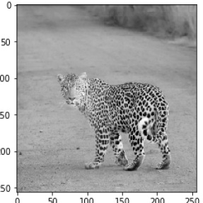
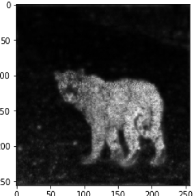
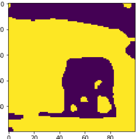
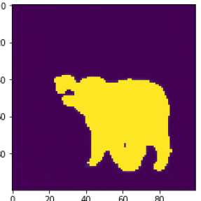
Fig. 2: Importance of pre-filtering. From left to right: original image, feature map representing a linear combination of Gabor filtered images, Algorithm 1

applied to the original input, and Algorithm 1 applied to the feature map.

Importance of pre-filtering

We start by a simple example that demonstrates the relevance of pre-filtering. The first two pictures in Fig. 2 show the original image and the feature map obtained by applying a Gabor filter (see Tab-1), where the aim is to segment the Leopard. The last two pictures in Fig. 2 show the resulting minimizers of the one-channel version of (2.1) applied to the original image and the feature map, respectively. Clearly, the segmentation map obtained from the filtered image better captures the Leopard to be segmented. It is also worth mentioning that the filtering approach comes with great flexibility. By applying different filters, one can emphasis different structures and different scales in order to target specific image content.

Table 2: Pre-filtering parameters for the texture images; again the feature maps are obtained by summing all filtered images.

Region	$\phi_{1}$	$\phi_{2}$	$\phi_{3}$	$\phi_{4}$
Brodatz 3	$n=2,3\colon(0,\frac{2^{n+1/2}}{256})$	$n=4,5\colon(\frac{\pi}{4},\frac{2^{n+1/2}}{256})$	$n=1,2\colon\frac{\pi}{4},\frac{2^{n+1/2}}{256})$	(none)
	$n=4\colon(\frac{\pi}{4},\frac{2^{n+1/2}}{256})$	$n=3,5\colon(\frac{3\pi}{4},\frac{2^{n+1/2}}{256})$	$n=2\colon(\frac{\pi}{2},\frac{2^{n+1/2}}{256})$
	$n=4\colon(\frac{3\pi}{4},\frac{2^{n+1/2}}{256})$	$n=1\colon(\frac{3\pi}{4},\frac{2^{n+1/2}}{256})$
Brodatz 5	$n=4\colon(0,\frac{2^{n+1/2}}{256})$	$n=4\colon(0,\frac{2^{n+1/2}}{256})$	$n=1,2\colon(0,\frac{2^{n+1/2}}{256})$	$1-\phi_{1}$
	$n=4\colon(\frac{\pi}{4},\frac{2^{n+1/2}}{256})$	$n=3,4\colon(\frac{\pi}{4},\frac{2^{n+1/2}}{256})$	$n=2\colon(\frac{\pi}{4},\frac{2^{n+1/2}}{256})$	$-\phi_{2}$
	$n=4\colon(\frac{\pi}{2},\frac{2^{n+1/2}}{256})$	$n=3\colon(\frac{3\pi}{4},\frac{2^{n+1/2}}{256})$		$-\phi_{3}$
	$n=4\colon(\frac{3\pi}{4},\frac{2^{n+1/2}}{256})$

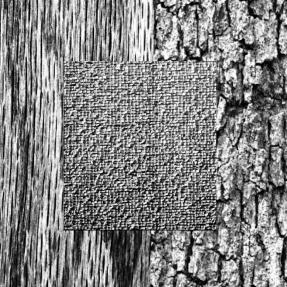
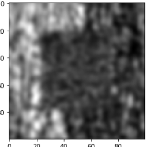
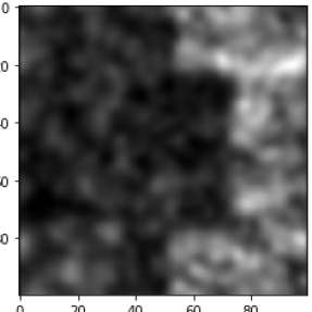
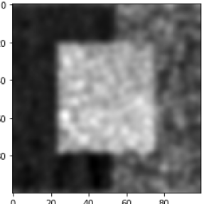
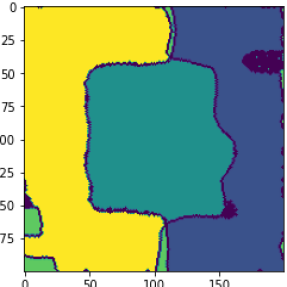
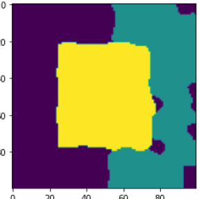
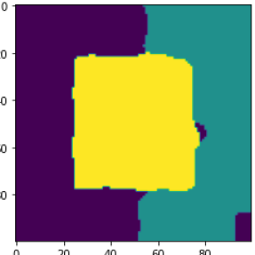
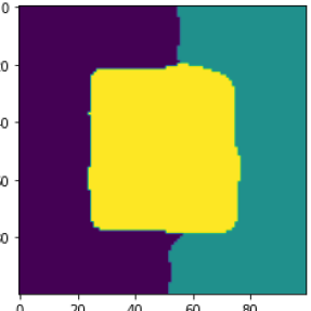
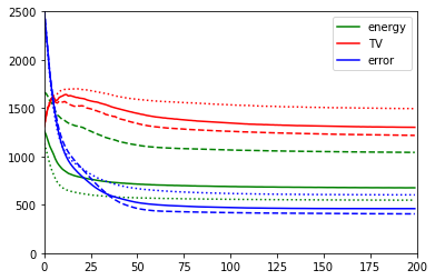
Fig. 3: Three-texture example. First row: Input image and extracted feature channels. Second row: Result with MMCV and

minimizers for $\lambda=0.1,0.2,0.5$ computed with Algorithm 1. Bottom: Evolution of TV, energy and absolute error over 200 iterations for $\lambda=0.1$ (dotted), $\lambda=0.2$ (solid) and $\lambda=0.5$ (dashed).

Three-texture example

The next example considers the segmentation of a texture image (top left picture in Fig. 3) consisting of three different Brodatz textures. The remaining pictures in the top row show the feature maps extracted via Gabor filtering. The second row shows the targeted ground truth segmentation and the minimizers computed with Algorithm 1 for different regularization parameters $\lambda$. The first image in the second row shows the results for MMCV with the regularization parameter $\lambda=0.4$, which has been empirically shown to give the best results. We compared different strategies for MMCV. For example, we used the grayscale image directly, which did not work. For this reason, we used the extracted feature maps in Fig. 3 and treated them as three different input channels. The second through fourth images in the second row show the minimizers computed using Algorithm 1 for different regularization parameters $\lambda$. The bottom row shows the evolution of energy, the TV semi-norm and the absolute error compared to the ground truth depending on the number of iterations. These results suggest that the parameter $\lambda$ not only accounts for the noise but also acts as a way to select a specific resolution of the segmentation task.

Table 3: Quantitative evaluation of segmentation results. These metrics are each calculated as means of the results obtained for different regions.

Method	Dice	Accuracy	Specificity	Recall	Precision
Brodatz 3
Ours	0.956	0.974	0.980	0.964	0.954
MMCV	0.924	0.954	0.980	0.908	0.950
Abscess
Ours	0.739	0.975	0.989	0.649	0.930
MMCV	0.566	0.941	0.980	0.594	0.573

4.2 Comparison with other algorithm

Next, we present comparison with other variational segmentation methods. Specifically, we compare our method with channel-wise Chan-Vese segmentation [24], its convex relaxation [11], and with the multichannel multiclass Chan-Vese (MMCV) model [12]. A quantitative evaluation of the compared algorithms can be found in Table 3. In these examples, our method performs better than MMCV.

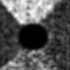
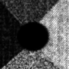
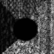
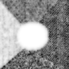
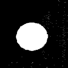
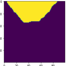
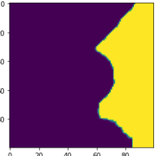
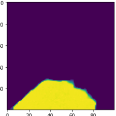
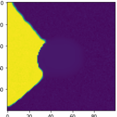
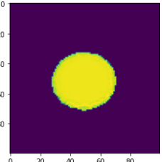
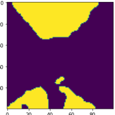
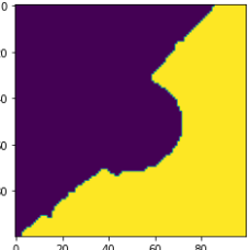
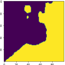
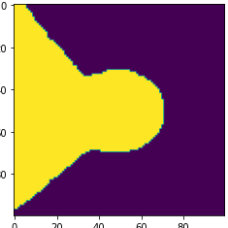
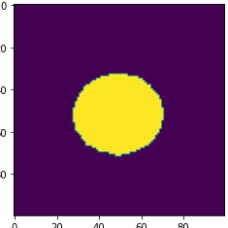
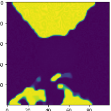
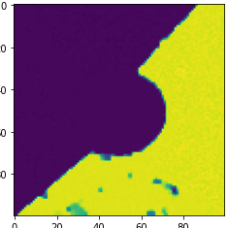
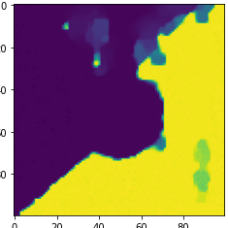
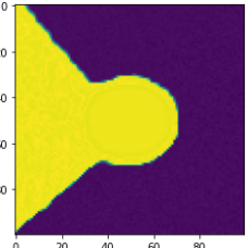
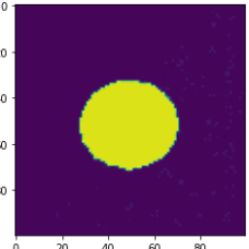
Fig. 4: Comparison with channel-wise (convex) Chan-Vese. First row: Feature maps obtained via Gabor filtering and thresholding. Second row: Proposed method. Third row: Channel wise Chan-Vese. Fourth row: Channel wise convex Chan-Vese. All experiments use $\lambda=0.1$.

A first comparison is shown in Fig. 4, where we use $K=5$ feature maps via Gabor filtering and simple thresholding. The pre-filtered images slightly highlight the five different texture regions, but again there are many overlaps and holes. The minimizer of the proposed functional (1.1) is depicted in the second row of Fig. 4. The third and fourth row, respectively, show results with the Chan-Vese model and its convex relaxation applied to each channel separately. Results clearly show the importance of the constraint preventing the results from overlapping.

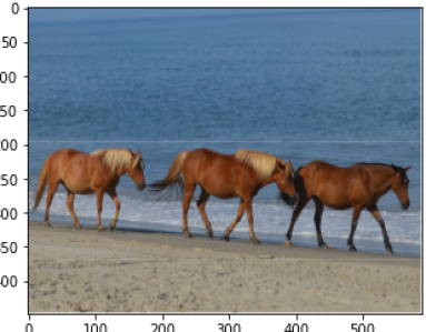
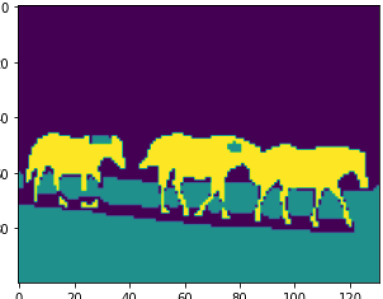
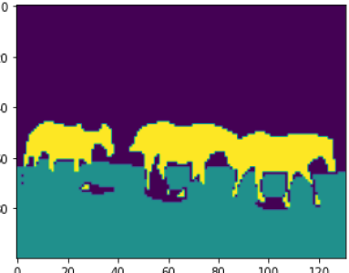
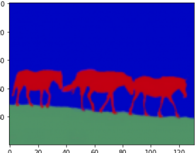
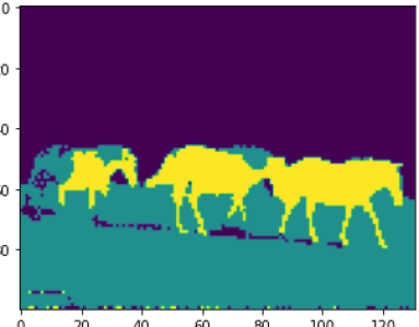
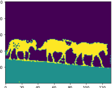
Fig. 5: Comparison with MMCV: Left: input image and groundtruth segmentation

. The remaining pictures show segmentation results for two different values of the regularization parameter using the proposed method (middle) and the MMCV model (right).

Another comparison is presented Fig. 5. In this example, the original input is an RGB image, so we have three channels serving as input of the proposed functional. The middle column shows results with the proposed method and the right column results with the MMCV model using the MATLAB-implementation provided by Wu [25]. Both methods achieve acceptable results, although those of the proposed method look slightly smoother.

4.3 Medical applications

The proposed framework can be directly applied to various medical imaging applications where the different channels naturally result from different imaging techniques. Our multichannel multiclass functional uses the information contained in the different categories of MRI and CT images or images resulting from different modalities, and can therefore divide the input image naturally into $K$ non-overlapping sub-regions.

As a first example, we consider a neuroradiological application, where we aim for dividing MRI images showing an abscess into the regions healthy, abscess and edema. The left column in Fig. 6 shows three channels of an MRI dataset using diffusion weighted imaging (DWI), apparent diffusion coefficient (ADC), and T2 sequence. As preprocessing, the ADC maps and T2 images were windowed and standardized to have intensity values between $[0,1]$. The second column shows the segmentations obtained by MMCV. Here we chose a weighted linear combination of the three images as the input image. This strategy was found to provide better results than treating the three images as separate channels. We selected the regularization parameter empirically so that it led to the best results. The remaining columns of Fig. 6 show the segmentation masks corresponding to four different regularization parameters. Smaller values of $\lambda$ result in quite inaccurate results containing many false positives. The results in the last row, which were obtained by setting the regularization parameter to $\lambda=0.2$, show an improvement compared to the ones in the previous columns. Quantitative evaluation metrics are summarized in Table 3.

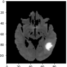
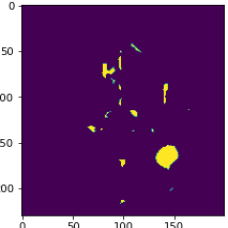
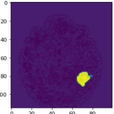
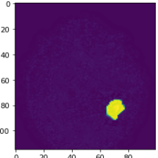
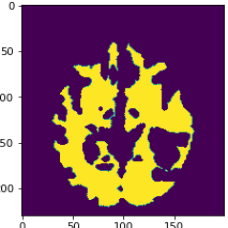
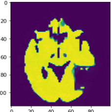
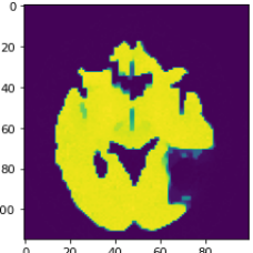
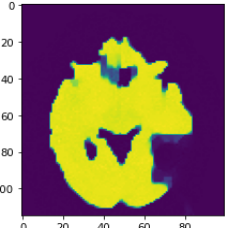
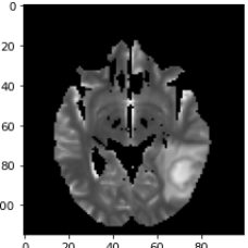
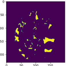
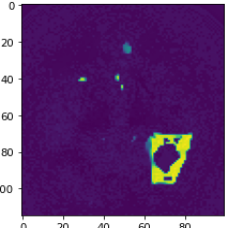
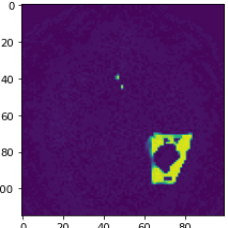
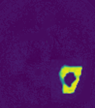
Fig. 6: Abscess in multichannel MRI data. Left column: DWI, ADC and T2 image of the same brain. Second column: results with MMCV. Remaining columns: Proposed method for different choices of $\lambda$. From top to bottom, the segmentation masks for abscess (top), healthy brain tissue (middle) and the edema (bottom) are visualized..

For the second medical example, we use image from the brain tumor segmentation (BRATS) challenge 2015 dataset; see https://www.smir.ch/BRATS/Start2015. The channels in this case consist of contrast-enhanced T1-weighted (T1c), T2 and fluid attenuated inversion recovery (FLAIR) images. Channels contain complementary information allowing accurate diagnosis and quantification of tumor growth. The top row in Fig. 7 shows the input images highlighting a different region of the tumor. Again, we exploit the information contained in different sequences by employing them as separate input channels. The proposed method is thus able to use this complementary information to delineate the different tissues and demonstrates solid results for this concrete example from medicine. The fact that the proposed energy functional can be applied directly to the given images, makes it particularly suitable for medical image segmentation.

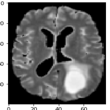
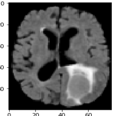
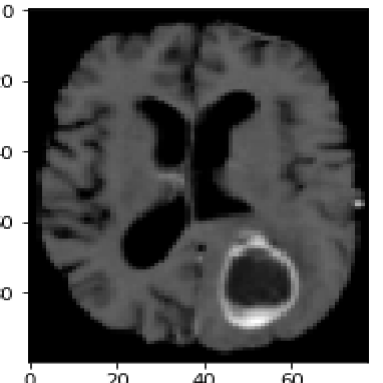
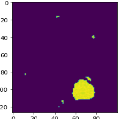
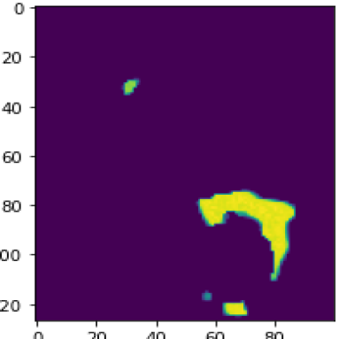
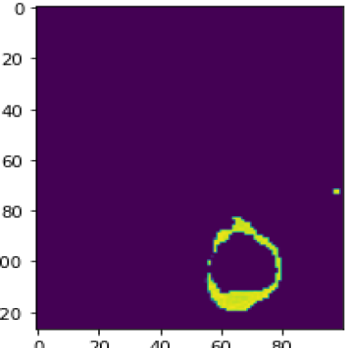
Fig. 7: Tumor growth example. Top row: T1c, T2 and FLAIR from same brain from BRATS dataset. Bottom row: Segmentation results for tumor(left), edema (middle) and necrosis (right).

5 Conclusion

In this paper, we have proposed a framework for variational image segmentation using feature map lifting and minimizing a multichannel segmentation functional. Input channels can be given either in a natural form, such as RGB images, or can be extracted by some pre-filtering method. We demonstrated the effectiveness of our method on several images, such as texture images or multi-modal medical images, and achieved convincing results also in comparison with related variational approaches. The method can distinguish a number of different regions, and is particularly suitable for applications in medical imaging. As main theoretical result, we have shown existence, stability and convergence with respect to the distorted input data. For future extension of the proposed framework, the combination with deep learning is planned, in particular, the feature maps extracted in this paper by means of pre-filtering might be obtained by a neural network. The combination of the strengths of modern deep learning and classical energy based segmentation methods could further improve the existing results, and enable more complex problems to be solved. In addition, a detailed comparison with other segmentation methods that also utilize feature lifting will be conducted.

The identification of appropriate feature maps is the main step in the proposed framework and is considered as its main current limitation. In order to obtain practically realistic results, the specific lifting has a significant impact on the final segmentation results. In this work, we focus on textured images, where the appropriate pre-filtering can be selected manually. In a recent follow-up work, we have proposed an automated lifting using convolutional networks [26]. Modern self-supervised deep learning methods, together with appropriate loss functions, can be used to obtain reasonable image decompositions. For example, in [26], a loss function that minimizes the correlation between different feature maps, along with a norm constraint on the feature maps, has been applied. Even with this, it is still somewhat unclear which segmentation is actually targeted by the lifting. To overcome this limitation, in future work. we plan to incorporate user guidance by allowing the user to roughly select representative regions for the different classes provided, in order to provide realistic results. It should also be noted that in the current setting, the pre-filtering should ensure a good separation of the channels.

List of Acronyms

ADC	Apparent diffusion coefficient
BRATS	Brain tumor segmentation
BV	Bounded variation
CT	Computed tomography
DWI	Diffusion weighted imaging
FLAIR	Fluid attenuated inversion recovery
MMCV	Multichannel multiclass Chan-Vese
MRI	Magnetic resonance imaging
PDHG	Primal-dual hybrid gradient
RGB	Red green blue
TV	Total variation
T1c	Contrast-enhanced T1-weighted image

References

- [1] J.-M. Morel, S. Solimini, Variational methods in image segmentation: with seven image processing experiments, Vol. 14, Springer Science & Business Media, 2012.
- [2] D. B. Mumford, J. Shah, Optimal approximations by piecewise smooth functions and associated variational problems, Commun. Pure Appl. Math. (1989).
- [3] O. Scherzer, M. Grasmair, H. Grossauer, M. Haltmeier, F. Lenzen, Variational methods in imaging, Springer, 2009.
- [4] T. F. Chan, L. A. Vese, Active contours without edges, IEEE Trans. Image Process. 10 (2) (2001) 266–277.
- [5] D. R. Martin, C. C. Fowlkes, J. Malik, Learning to detect natural image boundaries using local brightness, color, and texture cues, IEEE Trans. Pattern Anal. Mach. Intell. 26 (5) (2004) 530–549.
- [6] T. Randen, J. H. Husoy, Filtering for texture classification: A comparative study, IEEE Trans. Pattern Anal. Mach. Intell. 21 (4) (1999) 291–310.
- [7] M. Rousson, T. Brox, R. Deriche, Active unsupervised texture segmentation on a diffusion based feature space, in: 2003 IEEE Computer Society Conference on Computer Vision and Pattern Recognition, 2003. Proceedings., Vol. 2, IEEE, 2003, pp. II–699.
- [8] E. Bae, E. Merkurjev, Convex variational methods on graphs for multiclass segmentation of high-dimensional data and point clouds, J. Math. Imaging Vis. 58 (3) (2017) 468–493.
- [9] M. Kiechle, M. Storath, A. Weinmann, M. Kleinsteuber, Model-based learning of local image features for unsupervised texture segmentation, IEEE Trans. Image Process. 27 (4) (2018) 1994–2007.
- [10] M. Storath, A. Weinmann, M. Unser, Unsupervised texture segmentation using monogenic curvelets and the potts model, in: 2014 IEEE International Conference on Image Processing (ICIP), IEEE, 2014, pp. 4348–4352.
- [11] T. F. Chan, S. Esedoglu, M. Nikolova, Algorithms for finding global minimizers of image segmentation and denoising models, SIAM J. Appl. Math. 66 (5) (2006) 1632–1648.
- [12] L. A. Vese, T. F. Chan, A multiphase level set framework for image segmentation using the mumford and shah model, Int. J. Comput. Vis. 50 (3) (2002) 271–293.
- [13] C. Zach, D. Gallup, J.-M. Frahm, M. Niethammer, Fast global labeling for real-time stereo using multiple plane sweeps, in: VMV, 2008, pp. 243–252.
- [14] N. Mevenkamp, B. Berkels, Variational multi-phase segmentation using high-dimensional local features, in: 2016 IEEE Winter Conference on Applications of Computer Vision (WACV), IEEE, 2016, pp. 1–9.
- [15] T. Valkonen, A primal–dual hybrid gradient method for nonlinear operators with applications to mri, Inverse Problems 30 (5) (2014) 055012.
- [16] M. Storath, A. Weinmann, Fast partitioning of vector-valued images, SIAM J. Imaging Sci. 7 (3) (2014) 1826–1852.
- [17] E. Giusti, Minimal surfaces and functions of bounded variation, Monogr. Math. 80 (1984).
- [18] L. Ambrosio, N. Fusco, D. Pallara, Functions of bounded variation and free discontinuity problems, Vol. 254, Clarendon Press Oxford, 2000.
- [19] L. C. Evans, R. F. Gariepy, Measure theory and fine properties of functions, Vol. 5, CRC press Boca Raton, 1992.
- [20] A. Chambolle, T. Pock, A first-order primal-dual algorithm for convex problems with applications to imaging, J. Math. Imaging Vis. 40 (1) (2011) 120–145.
- [21] C. Michelot, A finite algorithm for finding the projection of a point onto the canonical simplex of , J. Optim. Theory Appl. 50 (1) (1986) 195–200.
- [22] A. K. Jain, F. Farrokhnia, Unsupervised texture segmentation using gabor filters, Pattern recognition 24 (12) (1991) 1167–1186.
- [23] K. Hammouda, E. Jernigan, Texture segmentation using gabor filters, Cent. Intell. Mach 2 (1) (2000) 64–71.
- [24] T. F. Chan, B. Y. Sandberg, L. A. Vese, Active contours without edges for vector-valued images, J. Vis. Commun. Image Represent. 11 (2) (2000) 130–141.
- [25] Y. Wu, Chan Vese Active Contours without edges, https://www.mathworks.com/matlabcentral/fileexchange/23445-chan-vese-active-contours-without-edges, [Online; accessed 22-June-2021] (2021).
- [26] N. Gruber, J. Schwab, S. Court, E. Gizewski, M. Haltmeier, Variational multichannel multiclass segmentation using unsupervised lifting with cnns, arXiv:2302.02214 (2023).