A tale of tails through generalized unitarity

Abstract

We introduce a novel framework to study high-order gravitational effects on a binary from the scattering of its emitted gravitational radiation. Here we focus on the radiation-reaction due to the background of the binary’s gravitational potential, namely on the so-called tail effects, as the starting point to this type of scattering effects. We start from the effective field theory of a binary composite-particle. Through multi-loop and generalized-unitarity methods, we derive the causal effective actions of the dynamical multipoles, the energy spectra, and the observable flux, due to these effects. We proceed through the third subleading such radiation-reaction effect, at the four-loop level and seventh order in post-Newtonian gravity, shedding new light on the higher-order effects, and pushing the state of the art.

Introduction.

Since the first detection of gravitational waves (GWs) from a black-hole binary merger [1] by the Advanced LIGO [2] and VIRGO [3] collaboration, we have been rapidly shifting to a new era of gravitational-wave astronomy. At present we already have a worldwide network of second-generation ground-based GW experiments, including the twin Advanced LIGO detectors in the US, Advanced Virgo in Europe [3], and the more recent KAGRA in Japan [4]. This network is planned to quickly expand, and provide a steeply increasing influx of GW data of ever-higher quality [5, 6, 7].

These exciting developments on the experimental frontier go hand in hand with a thrust in the theoretical frontier to push the program of high-precision gravity. For present GW sources the inspiral phase, in which typical velocities of the compact objects are non-relativistic, has been studied analytically via the post-Newtonian (PN) approximation of General Relativity [8]. PN gravity forms the basis for theoretical generation of gravitational waveforms, to be matched against measured data. This analysis is not only probing new astrophysics and cosmology, but also new fundamental physics, such as strong gravity and QCD in extreme conditions, which cannot be produced on Earth [9].

The surge in efforts to push the state of the art in PN gravity in the conservative sector has culminated at the fifth PN (5PN) order: The point-mass potential was accomplished via a combination of traditional GR methods [10, 11, 12], and via the effective field theory (EFT) approach [13, 14], and the complete quadratic-in-spin interactions were accomplished via the EFT of spinning objects [15, 16, 17]. The completion of amplitude and phasing of radiation at the +4PN order (4PN orders beyond leading) is also currently underway [8]. Notably at these high orders there is an intricate class of effects that come into play, which affect both the conservative and radiative sectors. These effects are the scattering of the binary’s emitted radiation off its own background.

This scattering exerts radiation-reaction forces on the binary, and contributes to the radiated energy-flux and to the binding energy of the binary. While leading radiation that yields a radiation-reaction force at the 2.5PN order contributes only to the radiated flux, the subleading effect that first involves such scattering, the so-called “tail”, enters at the 4PN order and already further affects the conservative dynamics. Such leading tail effects have been studied for a few decades now using traditional GR methods [18, 19, 20, 21, 22], which were extended to the next two subleading non-linear orders, the so-called “tail of tail” (TT) and “tail of tail of tail” (TTT), in [23, 24] and [25], respectively.

More recently, these effects have been studied via EFT methods, through two different approaches. One approach involves the one-point function of the stress-energy tensor as probed by an emitted on-shell radiation graviton [26], and proceeded through to the TT non-linear order. The other approach, which was led by Galley [27, 28, 29], also provides the radiation-reaction forces on the binary. The latter was applied to the leading radiation-reaction, namely without scattering [30, 31], and proceeded only to the leading tail effect [32]. Very recently, the subleading tail effects at 5PN order have been approached in [33, 34, 35] and [36].

In this letter we introduce a novel framework to study such higher-order gravitational effects due to the scattering of radiation. First, we note that at the radiation scale the scattered gravitons can go on-shell, which naturally aligns with scattering-amplitudes methods. This is unlike the situation in two-body conservative interactions, where the exchanged gravitons can never go on-shell. Using amplitudes methods at the orbital scale also alleviates the escalating complications of standard EFT methods with Feynman calculus involving the mixing of orbital and radiation modes.

The main idea that we put forward for the first time here is to think of the whole binary in analogy to elementary massive particles with gravitons scattered off of them. This is inspired by long-observed analogies of gravitational interactions of $l$-th mulitpole moments of a macroscopic object in effective theories of gravity, to gravitational scattering amplitudes with massive elementary particles of spin $l/2$, see e.g. [37, 15], and review in [16]. Let us highlight though that the various amplitudes-driven approaches that followed the latter, initiated in [38, 39, 40, 41], and recently reviewed in [42], implement their methods on single compact objects as elementary particles (and off-shell gravitions as noted), and thus have been tied to a treatment of the unbound problem of scattering two massive objects instead of the actual bound problem of the binary inspiral.

In contrast, we advocate an entirely orthogonal approach. By treating the whole binary as elementary massive particles our derivations lie directly in the binary inspiral problem and in PN theory, and are consequently directly applicable to present and planned GW experiments and measurements. In addition, a connection of those previous approaches from the unbound to the bound problem seems to become infeasible, even in restricted configurations, exactly when radiation-reaction effects – which we target in the novel formulation in this letter – show up [42]. Moreover, given the current state of the art we need to push these effects to high non-linear orders, which amounts to higher loops in QFT. Unlike previous works [42], in our present approach we do not invoke the propagation of quantum DOFs, which would in turn have to be laboriously excised from the meaningful classical contributions. Rather we only work with classical propagating DOFs, which keeps our formulation considerably lighter, and thus more efficient for the problem at hand.

In this letter we focus on scattering due to the binary’s gravitational potential, namely on tail effects, as the staring point to tackle this generic type of radiation-scattering effects. We start from the EFT of a binary as composite particle, and use multi-loop integration [43, 44] and generalized-unitarity methods [45, 46, 47, 48], to set up a basis-unitarity inspired procedure to treat such effects, assembling pure tree amplitudes generated by the public code IncreasingTrees [49] as building blocks. Since time reversal no longer holds we invoke the closed time path (CTP) formalism, which we extend to our new framework, and take a radiation-reaction approach in order to uniquely capture the entirety of effects – on both conservative and dissipative sides. We derive here the causal effective action of the dynamical multipoles, the energy spectrum, and the observable flux due to these effects. We proceed through the third subleading effect, at the 4-loop level and 7PN order, shedding new light on these higher-order effects, and pushing the state of the art.

From a binary-particle EFT to generalized unitarity.

We start by recalling the effective action of a composite object coupled to the gravitational field, $g_{\mu\nu}\equiv\eta_{\mu\nu}+h_{\mu\nu}$, that reads [26, 50, 16]:

$$S_{\text{eff(c)}}[g_{\mu\nu},y_{c}^{\mu},e_{c\,A}^{\,\,\mu}]= -\frac{1}{16\pi G}\int d^{4}x\sqrt{g}\,R\left[g_{\mu\nu}\right]$$

$$+\,S_{\text{pp(c)}}[g_{\mu\nu}(y_{c}),y_{c}^{\mu},e_{c\,A}^{\,\,\mu}](\sigma_{c}),$$ (1)

where $S_{\text{pp(c)}}$ is the worldline point-particle action of the composite particle with the form [26, 51, 50, 16]:

$$S {}_{\text{pp(c)}}[h_{\mu\nu},y_{c}^{\mu},e_{c\,A}^{\,\,\mu}](t)=-\int dt\sqrt{g_{00}}\,\biggr{[}E(t)$$

$$+ \frac{1}{2}\epsilon_{ijk}J^{k}(t)\left(\Omega_{\text{LF}}^{ij}+\omega_{\mu}^{ij}u^{\mu}\right)-\sum_{l=2}^{\infty}\biggr{(}\frac{1}{l!}I^{L}(t)\nabla_{L-2}\mathcal{E}_{i_{l-1}i_{l}}$$

$$- \frac{2l}{(l+1)!}J^{L}(t)\nabla_{L-2}\mathcal{B}_{i_{l-1}i_{l}}\biggr{)}\biggr{]},$$ (2)

where here the worldline parameter is the time coordinate, $t$. $E$ here is the total energy of the composite object, and $I^{L}$ and $J^{L}$ are definite-parity $SO(3)$ tensors, with the superscript $L$ for the indices $i_{1}\cdots i_{l}$ ($l\geq 2$) in the Euclidean metric. They are coupled to the electric $\mathcal{E}$ and magnetic $\mathcal{B}$ components of the Riemann tensor, respectively. For the present work we only need to consider the total energy, and the leading quadrupole moment, $I_{ij}$.

As the system is radiating and the symmetry of time reversal is broken, the closed time path (CTP) formalism needs to be invoked [52, 27, 16], to integrate out the gravitational field from (From a binary-particle EFT to generalized unitarity.). This yields a new causal effective action of the binary multipoles, from which the radiation-reaction forces and the energy spectrum of emitted radiation can be derived. To switch onto the CTP formalism all degrees of freedom (DOFs) are formally doubled, and the action is defined as:

$$S_{\text{CTP}}[\{\}_{1},\{\}_{2}]\equiv S[\{\}_{1}]-S^{*}[\{\}_{2}],$$ (3)

where $\{\}$ denotes the set of all DOFs in the original action, $S[\{\}]$. For the doubled DOFs it is convenient to switch to the $\{+,-\}$ basis, which for classical fields entails the propagator matrix with the $\{+,-\}$ labels: $G_{++}=G_{--}=0$, $G_{+-}=G_{adv}$, $G_{-+}=G_{ret}$, where the retarded and advanced propagators are given by

$$G_{ret/adv}(x-x^{\prime})=\int\frac{d^{D}p}{(2\pi)^{D}}\frac{e^{-ip_{\mu}(x-x^{\prime})^{\mu}}}{(p_{0}\pm i\epsilon)^{2}-\vec{p}\,{}^{2}},$$ (4)

namely the $+$ or $-$ $i\epsilon$ prescription for the retarded or advanced propagator, respectively, and $D\equiv d+1$ with $d$ for the number of spatial dimensions.

In the standard EFT approach the gravitational field is integrated out using Feynman diagrammatic expansion. Figures 1.1a, 1.2a, 2.a, and 3.a show example Feynman graphs that would need to be evaluated. Due to the non-relativistic context, the integration is over 3-dimensional spatial momenta, where the frequency of emitted radiation, $\omega$, is regarded as the mass scale of such Euclidean propagators. According to the generalized-unitarity paradigm, such Feynman integration can be equivalently accounted for by writing the resulting effective action as a linear combination:

$$S_{\text{eff}}=\int\frac{d\omega}{2\pi}\sum_{i\in\text{MI}}c_{i}\mathcal{I}_{i},$$ (5)

where $\{\mathcal{I}_{i}\}$ are a complete set of master integrals that span the integral family of the problem, and the coefficients ${c}_{i}$ are rational functions of the dimension $d$ and scales of the problem, which in our case is only the frequency. To fix the coefficients ${c}_{i}$ we will evaluate the cuts that span this complete set of integrals.

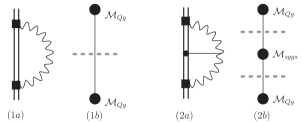
Figure 1: Radiation-reaction and tail effects from the EFT and amplitudes perspectives. (1a), (2a): The Feynman graphs of maximal propagators, which contain all invariants of loop momenta. The double line represents the worldline of the binary particle, the squares represent quadrupole couplings, and the wiggly line represents the radiation graviton emitted. The circle stands for the energy coupling, and the straight line for a potential graviton. (1b), (2b): The amplitude cuts used to evaluate the radiation reaction and tail effects. The black circles represent tree amplitudes with massive particles, including a 4-particle amplitude of 2 scalars and 2 gravitons, sggs, and the solid lines cut by dashed lines stand for the graviton-state sewing of the cut.

We illustrate how this new method works by treating radiation-reaction and tail effects at increasing loop orders. First, we approach radiation-reaction, depicted in figure 1. We start by considering the Feynman graphs with the maximal number of propagators that contain all possible invariants of loop momenta. Radiation reaction has only one loop and thus one invariant, captured by the single graph in figure 1.1a. The integral family at one-loop order is then simply:

$$F^{(1)}(\lambda;\omega^{2}) =\int\frac{\mathop{}\!\mathrm{d}^{d}\ell_{E}}{(2\pi)^{d}}\frac{1}{(-\ell_{E}^{2}+\omega^{2})^{\lambda}}$$

$$=R(d,\lambda,\omega^{2n(\lambda)})F^{(1)}(1;\omega^{2})\,,$$ (6)

where for integer $\lambda$, $R$ is a rational function, with leading power of $\omega$ set by $\lambda$, and thus $F^{(1)}(1;\omega^{2})$ is the master integral at one-loop order. We can then write the effective action as

$$S_{\text{RR}}=\int\frac{\mathop{}\!\mathrm{d}\omega}{2\pi}c_{\text{RR}}(\omega)F^{(1)}(1;\omega^{2})\,,$$ (7)

with $c_{\text{RR}}$ the coefficient to be fixed from unitarity cuts. Here we only need to evaluate one cut, as in figure 1.1b.

Our cuts are assembled from tree amplitudes as building blocks, contracted via graviton-state sewing, which inserts the relation:

$$\sum_{\text{states}} \varepsilon^{\mu\nu}_{k}\varepsilon^{\alpha\beta*}_{k}\equiv\mathcal{P}^{\mu\nu;\alpha\beta}_{k}$$

$$=\frac{1}{2}\left(P_{k}^{\mu\alpha}P_{k}^{\nu\beta}+P_{k}^{\mu\beta}P_{k}^{\nu\alpha}-\frac{1}{D-2}P_{k}^{\mu\nu}P_{k}^{\alpha\beta}\right),$$ (8)

in which $P^{\mu\nu}_{k}\equiv\eta^{\mu\nu}-\frac{k^{\mu}q^{\nu}+k^{\nu}q^{\mu}}{k\cdot q},$ and $q$ is an arbitrary null reference momentum, of which all dependence eventually cancels in any cut due to gauge invariance [53]. For the quadrupole coupling to the graviton, we make the following definition:

$$\mathcal{M}_{Qg}\equiv\lambda_{Q}J^{\mu\nu}\epsilon_{\mu\nu}\equiv\lambda_{Q}J^{\mu\nu}\varepsilon_{\mu}\varepsilon_{\nu}=-\lambda_{Q}I^{ab}$$

$$\hskip 5.0pt\times\left(k_{0}k_{a}\varepsilon_{0}\varepsilon_{b}+k_{0}k_{b}\varepsilon_{0}\varepsilon_{a}-k_{a}k_{b}\varepsilon_{0}\varepsilon_{0}-k_{0}k_{0}\varepsilon_{a}\varepsilon_{b}\right)\,,$$ (9)

with leading couplings only, and $\lambda_{Q}\equiv\sqrt{2\pi G_{N}}$. The cut in figure 1.1b is then assembled as:

$$\mathcal{C}_{\text{RR}} =\lambda_{Q}^{2}J_{1}^{\mu\nu}\ \mathcal{P}^{\mu\nu;\alpha\beta}J_{2}^{\alpha\beta}\Big{|}_{P_{\ell}=\ell_{E}^{2}-\omega^{2}=0}$$

$$=\delta(\ell_{E}^{2}-\omega^{2})\lambda_{Q}^{2}\left(J_{1}^{\mu\nu}J_{2}^{\mu\nu}-\frac{J_{1}^{\mu\mu}J_{2}^{\nu\nu}}{d-1}\right)\,,$$ (10)

which evaluates to

$$\mathcal{C}_{\text{RR}}=\delta(P_{\ell})\lambda_{Q}^{2}\frac{(d+1)(d-2)}{(d+2)(d-1)}\omega^{4}\kappa_{ab}(\omega)\,,$$ (11)

where $\kappa_{ab}(\omega)=I^{ij}_{a}(-\omega)I_{ij,b}(\omega)$ with $a,b\in\{+,-\}$, is the trace of the CTP quadrupole DOFs.

The CTP effective action can then be written as

$$S_{\text{RR}} =\frac{2\pi G_{N}}{5}\int\frac{\mathop{}\!\mathrm{d}\omega}{2\pi}\,\omega^{4}\sum_{a,b\in\{+,-\}}\kappa_{ab}(\omega)F^{(1)}(1_{ab})\,,$$ (12)

with the retarded and advanced propagators, $F^{(1)}(1_{-+}/1_{+-})\equiv F^{(1)}(1;(\omega\pm i\epsilon)^{2})$, so that finally we obtain

$$S_{\text{RR}}=-i\frac{G_{N}}{5}\int_{-\infty}^{\infty}\frac{\mathop{}\!\mathrm{d}{\omega}}{2\pi}\,\omega^{5}I_{-}^{ij}(-\omega)I_{+,ij}(\omega)\,,$$ (13)

in agreement with Galley et al. in [31, 32], whose action is given in time domain, and up to an overall sign discrepancy between the two references [31, 32] – we agree with the latter.

Let us proceed to the tail effect that is captured by the single Feynman graph depicted in figure 1.2a. The “integer-indexed” integral family that contains the 3 invariants constructed out of the 2 loop momenta reduces, using FIRE6 [44], to a master integral of only two propagators for the two loops:

$$F^{(2)}(1_{X},1_{Y},0) =\int\frac{\mathop{}\!\mathrm{d}^{d}\ell_{1}\mathop{}\!\mathrm{d}^{d}\ell_{2}}{(2\pi)^{2d}}\frac{1}{(-\ell_{1}^{2}+\omega^{2}_{X})(-\ell_{2}^{2}+\omega^{2}_{Y})}$$

$$=F^{(1)}(1;\omega_{X}^{2})F^{(1)}(1;\omega_{Y}^{2})\,,$$ (14)

where the entries in $F^{(2)}$ stand for exponents of the 3 denominators that span the generic integral family, and $X$, $Y$ label different possible $i\epsilon$ prescriptions. We can then write for the tail effective action:

$$S_{\text{T}}=\int\frac{\mathop{}\!\mathrm{d}\omega}{2\pi}c_{\text{T}}(\omega)F^{(2)}(1_{X},1_{Y},0)\,.$$ (15)

To assemble the cut that corresponds to this master integral and determine $c_{\text{T}}$, we take a tree amplitude of 2 massive scalars and 2 gravitons as a building block, corresponding to the binary’s energy $E$, coupling to two gravitons. This is where we use the analogy between the coupling of the binary’s mass monopole to gravity and the gravitational scattering of massive scalar particles. The above amplitude can be extracted from [49], and since in the non-relativistic limit $|\vec{k}|,|\vec{p}|\ll m_{s}$, it is then expanded in the large-mass limit as:

$$\mathcal{M}_{sggs}(m_{s}\to\infty)= \frac{\lambda_{g}\lambda_{E}}{\omega_{k_{2}}^{2}}\frac{1}{2(k_{2}^{\mu}k_{3,\mu})}\Big{[}(k_{2}^{\mu}k_{3,\mu})\varepsilon_{2}^{0}\varepsilon_{3}^{0}$$

$$+\omega_{k_{2}}((\varepsilon_{3}^{\mu}k_{2,\mu})\varepsilon_{2}^{0}-(\varepsilon_{2}^{\mu}k_{3,\mu})\varepsilon_{3}^{0})$$

$$-\omega_{k_{2}}^{2}(\varepsilon_{2}^{\mu}\varepsilon_{3,\mu})\Big{]}^{2}+\mathcal{O}(m_{s}^{-1}),$$ (16)

where 2 and 3 label the two gravitons, and $\lambda_{E}$ is fixed from the 3-particle tree amplitude of 2 massive scalars and a graviton, $\mathcal{M}_{sgs}\equiv\lambda_{E}(p^{\mu}p^{\nu}/m_{s}^{2})\varepsilon^{\mu}\varepsilon^{\nu}$, so that $\lambda_{E}\equiv-\sqrt{8\pi G_{N}}E$. The graviton self-coupling, $\lambda_{g}\equiv-\sqrt{32\pi G_{N}}$, is similarly fixed from a 3-graviton amplitude [49]. With all the ingredients in place we can assemble the cut, shown in figure 1.2b, to fix the coefficient in (15):

$$\mathcal{C}^{(2)}_{1,1,0} =\sum_{\text{states}}\mathcal{M}_{Qg(-\omega)}\mathcal{M}_{sggs}\mathcal{M}_{Qg(\omega)}\Big{|}_{\begin{subarray}{c}P_{\ell_{1}}=0,P_{\ell_{2}}=0\\ m_{s}\to\infty\end{subarray}}$$

$$=\lambda_{Q}^{2}\,\delta(P_{\ell_{1}})\delta(P_{\ell_{2}})$$

$$\times J_{I(-\omega)}^{\mu\nu}P^{\mu\nu;\alpha\beta}\mathcal{M}_{sggs}^{\alpha\beta;\gamma\sigma}P^{\gamma\sigma;\rho\tau}J_{I(\omega)}^{\rho\tau}\Big{|}_{m_{s}\to\infty}\,.$$ (17)

Reducing the resulting integrals [44], and evaluating the master integrals with the appropriate CTP prescriptions, we finally find:

$$S_{\text{T}}=\frac{2}{5}G_{N}^{2}E \int\frac{\mathop{}\!\mathrm{d}\omega}{2\pi}\,\omega^{6}\kappa_{-+}(\omega)$$

$$\times\Bigg{[}\frac{1}{\epsilon_{d}}+\log\left(\frac{\omega^{2}}{\mu^{2}}\right)-i\pi\operatorname*{sgn}(\omega)\Bigg{]},$$ (18)

with $\epsilon_{d}\equiv d-3$, and in agreement with equation (3.4) of Galley et al., up to an overall sign discrepancy [32]. The coefficient of the dimensional-regularization (DimReg) pole is even in $\omega$. When mapped from the $\{+,-\}$ to the $\{1,2\}$ CTP basis, terms that are even in $\omega$ lead to a separated action for the quadrupoles of the form eq. 3, and are thus conservative [28, 29]. Thus, as noted in [32] this DimReg pole renormalizes the binding energy. We also absorb constant terms that are at the same $\epsilon_{d}$ order as the logarithmic term into the logarithm scale $\mu$. We apply similar implicit suppression to the following higher-order results.

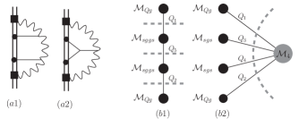
Figure 2: The tail-of-tail effect from the Feynman and amplitudes perspectives. All notations are similar to figure 1, with the grey circle for a 4-graviton tree amplitude. We similarly only include the Feynman graphs with cubic vertices, which are used to determine all allowed propagators.

We proceed to the tail-of-tail (TT) effect, for which no effective action has been previously derived. We start again by considering the Feynman graphs that contain the invariants from 3 loop momenta. In this case 2 graphs, shown in figure 2.a, suffice to contain all the invariants, which span the integral family at the 3-loop order:

$$F^{(3)}(\lambda_{1},\lambda_{2},\lambda_{3},\lambda_{4},\lambda_{5},\lambda_{6})$$

$$=\int\left(\prod_{i=1}^{3}\frac{\mathop{}\!\mathrm{d}^{d}\ell^{i}}{(2\pi)^{d}}\right)\frac{1}{Q_{1}^{\lambda_{1}}Q_{2}^{\lambda_{2}}Q_{3}^{\lambda_{3}}Q_{4}^{\lambda_{4}}Q_{5}^{\lambda_{5}}Q_{6}^{\lambda_{6}}}\,,$$ (19)

where the 6 invariants show up in the 6 denominators $\{Q_{i}\}$. For relevant integer values of $\lambda_{i}$ this integral is then reduced [44], and is found to be spanned by 2 master integrals, so that we can write the effective action of the TT effect as:

$$S_{\text{TT}}=\int\frac{\mathop{}\!\mathrm{d}\omega}{2\pi}\Big{[} c_{1}(\omega)F^{(3)}(1,1,0,0,1,0)$$

$$+ c_{2}(\omega)F^{(3)}(1,1,1,1,0,0)\Big{]}\,,$$ (20)

where again the 3-loop master integrals $F^{(3)}$ contain entries for exponents of the 6 denominators, and we now suppress the labels for various $i\epsilon$ prescriptions.

The 2 cuts that correspond to these 2 master integrals are shown in figure 2.b. The first cut in 2.b1 is assembled from building blocks that we already used in lower loop orders:

$$\mathcal{C}^{(3)}_{1,1,0,0,1,0}=\lambda_{Q}^{2}\,\delta(Q_{1})\delta(Q_{2})\delta(Q_{5})$$

$$\times J_{I(-\omega)}P\mathcal{M}_{sggs,1}P\mathcal{M}_{sggs,2} PJ_{I(\omega)}\Big{|}_{m_{s}\to\infty}\,,$$ (21)

where the sewing indices were suppressed for readability, and the resulting expression after evaluation is quite lengthy. The second cut in figure 2.b2 further requires the 4-graviton tree amplitude, $\mathcal{M}_{4}$, taken from [49], to which no special kinematics should be applied for our context. This cut is assembled as follows:

$$\mathcal{C}^{(3)}_{1,1,1,1,0,0}=\lambda_{Q}^{2}\,\delta(Q_{1})\delta(Q_{2})\delta(Q_{3})\delta(Q_{4})$$

$$\times(J_{I(-\omega)}P)(\mathcal{M}_{sgs,1}P)\mathcal{M}_{4}^{\text{tree}}(P\mathcal{M}_{sgs,2})(PJ_{I(\omega)})\,,$$ (22)

where again we suppress the contraction indices for readability. Plugging in the values of cuts and the appropriate CTP prescriptions, we finally find the CTP effective action of the TT effect:

$$S_{\text{TT}}=\frac{107}{175}\,G_{N}^{3}E^{2} \int\frac{\mathop{}\!\mathrm{d}\omega}{2\pi}\,\omega^{7}\kappa_{-+}(\omega)$$

$$\times\Bigg{[}\pi\operatorname*{sgn}(\omega) +i\left[\frac{2}{3\,\epsilon_{d}}+\log\left(\frac{\omega^{2}}{\mu_{1}^{2}}\right)\right]\Bigg{]}\,.$$ (23)

Unlike in the tail effective action, the DimReg pole is now non-conservative, as its coefficient is odd in $\omega$ leading to a CTP action that cannot be separated as in eq. 3 [28, 29]. Thus, it must be removed prior to extracting dissipative observables from the action. The most straightforward method of removal is to introduce a renormalized coupling to the quadrupole, similar to [26] (see Appendix).

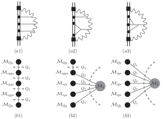
Figure 3: The tail-of-tail-of-tail effect from the Feynman and amplitudes perspectives. All notations and restrictions are similar to figures 1, 2. Graph a2 is also considered in its top-bottom mirror image, and graph b2 is evaluated as 2 cuts, which are swapped in a top-bottom mirror image.

Building on the procedure presented at lower loop orders, we briefly outline the derivation for the tail-of-tail-of-tail (TTT) effect, which proceeds along similar lines. There are 4 Feynman graphs, shown in figure 3.a, that span the integral family at the 4-loop order with 10 generic denominators. The relevant integrals are then reduced to 4 master integrals [44], so that the effective action of the TTT effect can be written as:

$$S_{\text{TTT}} =\int\frac{\mathop{}\!\mathrm{d}\omega}{2\pi}\Big{[}c_{1}\,F^{(4)}_{1,1,1,1,0,0,0,0,0,0}+c_{2}\,F^{(4)}_{1,0,0,1,1,1,1,0,0,0}$$

$$+\big{(} c_{3}\,F^{(4)}_{1,0,1,1,1,1,0,0,0,0}+c_{4}\,F^{(4)}_{1,1,0,1,0,1,1,0,0,0}\big{)}\Big{]}\,,$$ (24)

where the entries in $F^{(4)}$ are for exponents of the 10 denominators, and we suppress labels for various $i\epsilon$ prescriptions and dependence in $\omega$ of the coefficients $c_{i}$.

The 4 cuts that correspond to the 4 master integrals are shown in figure 3.b, where the cut $\mathcal{C}^{(4)}_{1,0,0,1,1,1,1,0,0,0}$ in 3.b3, further requires the 5-graviton tree amplitude, $\mathcal{M}_{5}$, taken from [49]. The cuts are then assembled as in the previous cases, and each is thousands of terms long to begin with. Substituting in the values of cuts and the proper CTP prescriptions, we arrive at the CTP effective action of the TTT effect:

$$S_{\text{TTT}}=-\frac{4}{525}G_{N}^{4}E^{3}\int\frac{\mathop{}\!\mathrm{d}\omega}{2\pi}\,\omega^{8}\kappa_{-+}(\omega)$$

$$\times\Bigg{[}\frac{107}{2\epsilon_{d}^{2}}+\frac{107}{\epsilon_{d}}\log\left(\frac{\omega^{2}}{\mu_{2}^{2}}\right)+107\log^{2} \left(\frac{\omega^{2}}{\mu_{2}^{2}}\right)$$

$$+\frac{20707426967}{60399360}-\frac{3103}{4}\,\zeta_{2}-420\, \zeta_{3}$$

$$-i\pi\operatorname*{sgn}(\omega)\Bigg{[}\frac{107}{\epsilon_{d}}+214\log\Big{(} \frac{\omega^{2}}{\mu_{2}^{2}}\Big{)}\Bigg{]}\,\Bigg{]}\,,$$ (25)

where $\zeta_{2}\equiv\pi^{2}/6$ and $\zeta_{3}$ is Apéry’s constant. The DimReg poles now appear in both the conservative and dissipative parts. The non-conservative pole can be removed by renormalizing quadrupoles in the tail action, using exactly the same renormalization scheme as in TT.

From CTP Effective Actions to Spectra and Fluxes.

It is useful to have the CTP effective actions in order to obtain the related radiation-reaction forces by varying with respect to the CTP DOFs, $\{q_{\pm}^{i}\}$, and then taking the physical limit, $q_{+}^{i}\to q^{i}$ and $q_{-}^{i}\to 0$. We defer a discussion of the conservative sector for future work.

We can extract the energy spectrum in the CTP formalism by starting from the generalized Noether theorem [29], which tells us that in the time domain:

$$\frac{\mathop{}\!\mathrm{d}E}{\mathop{}\!\mathrm{d}t}=-\frac{\partial L}{\partial t}+\dot{q}^{i}\left[\frac{\partial K}{\partial q_{-}^{i}}\right]_{\text{PL}}+\ddot{q}^{i}\left[\frac{\partial K}{\partial\dot{q}_{-}^{i}}\right]_{\text{PL}}+\ldots\,,$$ (26)

where $L$ is the conservative potential of one of the time histories, $K$ is the non-conservative potential, $\{q^{i}\}$ are the generalized coordinate variables or DOFs, and PL denotes the physical limit as noted, $q_{+}\to q$ and $q_{-}\to 0$. We then work out (26) with the CTP quadrupoles as our generalized DOFs, and if we then integrate over $t$, we arrive at

$$\int\mathop{}\!\mathrm{d}t\frac{\mathop{}\!\mathrm{d}E}{\mathop{}\!\mathrm{d}t}=\Delta E=\int\mathop{}\!\mathrm{d}\omega\frac{\mathop{}\!\mathrm{d}E}{\mathop{}\!\mathrm{d}\omega},$$ (27)

where on the right-hand side we have the energy spectrum that we want.

Applying our generic derivation to the tail actions is then straightforward. First, we obtain the energy spectrum of radiation reaction as:

$$\int_{0}^{\infty}\mathop{}\!\mathrm{d}{\omega}\frac{\mathop{}\!\mathrm{d}E_{\text{RR}}}{\mathop{}\!\mathrm{d}\omega}=-\frac{G_{N}}{5\pi}\int_{0}^{\infty}\mathop{}\!\mathrm{d}{\omega}\,\omega^{6}\kappa(\omega)\,,$$ (28)

where now $\kappa(\omega)\equiv I^{ij}(-\omega)I_{ij}(\omega)$. Similarly, we obtain the following power spectra:

$$\frac{\mathop{}\!\mathrm{d}E_{\text{T}}}{\mathop{}\!\mathrm{d}\omega} =-\frac{2}{5}G_{N}^{2}E\,\omega^{7}\kappa(\omega)\,,$$ (29)

$$\frac{\mathop{}\!\mathrm{d}E_{\text{TT}}}{\mathop{}\!\mathrm{d}\omega} =\frac{428\,\,}{525\pi}G_{N}^{3}E^{2}\,\omega^{8}\log(\omega/\mu_{1})\kappa(\omega)\,,$$ (30)

$$\frac{\mathop{}\!\mathrm{d}E_{\text{TTT}}}{\mathop{}\!\mathrm{d}\omega} =\frac{856}{525}G_{N}^{4}E^{3}\,\omega^{9}\log(\omega/\mu_{2})\kappa(\omega)\,,$$ (31)

for the tail, TT and TTT effects, respectively. (29) and (30) are in agreement with [54], and (31) is new.

As a final check, we can also specialize to a circular orbit with orbital frequency $\Omega$ to get the energy flux in terms of the symmetric mass ratio $\nu$, and the PN parameter $x=(\Omega G_{N}E)^{2/3}$. We then obtain:

$$P_{\text{RR}}^{\text{circ}}=-\frac{32}{5G_{N}}\nu^{2}x^{5},\quad P_{\text{T}}^{\text{circ}}=-\frac{128\pi}{5G_{N}}\nu^{2}x^{13/2}\,.$$ (32)

For the TT and TTT we present the non-analytic contributions:

$$P_{\text{TT}}^{\text{circ}}=\frac{27392}{175G_{N}}\nu^{2}x^{8}\ln x,\,\,\,P_{\text{TTT}}^{\text{circ}}=\frac{109568\pi}{175G_{N}}\nu^{2}x^{19/2}\ln x\,.$$ (33)

These results for the flux from a circular orbit are in complete agreement with [55, 56, 24, 8, 25].

Future prospects of the new unitarity framework.

In this letter we introduced a novel framework to tackle higher-order gravitational effects due to scattering of the binary’s emitted radiation from its own gravitational background. Within this framework we derive the causal effective actions of the dynamical multipoles, that encapsulate all conservative and dissipative physics, including those of the TT and TTT, that were never previously derived. We derive dissipative observables: first the generic energy spectra, and then the observed circular-orbit flux due to these effects. We find complete agreement with available results obtained via traditional GR and standard EFT methods. One can also derive the conservative dynamics from our actions, e.g. EOMs and binding energies. Given the current state of the art we set out to establish a framework which is able to push through these effects to higher PN orders. Here we proceeded through the third subleading such radiation-reaction effect, which corresponds to the 4-loop level and the 7PN order. This is shedding new light on these higher-order effects, and pushing the state of the art.

Our novel framework utilizes multi-loop and generalized-unitarity methods to set up an amplitudes-like computation which captures such radiation-scattering effects with high efficiency. In this letter we demonstrated that the new approach is already competitive with traditional GR methods, and even outpaces standard EFT methods, which become intractable already at subleading tail effects. Our framework constitutes the first direct application of modern amplitude methods to the binary inspiral problem and thus to present and planned GW measurements, in PN theory. Obvious extensions of this framework include subleading PN orders of the non-linear effects, and scattering of subleading radiation from generic multipole sources off background generated by generic multipole sources. Both entail tree amplitudes with massive particles of any spin, namely also of higher spins. As noted the framework presented here should be straightforward to apply to the conservative as well as the radiative sector. We leave all these developments for future work.

Appendix: Renormalizing Higher-Order Tails

The CTP effective actions in eqs. (From a binary-particle EFT to generalized unitarity.), (From a binary-particle EFT to generalized unitarity.), (From a binary-particle EFT to generalized unitarity.) contain DimReg poles, and go through a renormalization. As we illustrate below, there is an interplay among lower-order DimReg zeros and higher-order DimReg poles, similar to that in purely conservative effective potentials as of the N³LO sectors. The renormalization we apply is essentially similar to that in [26], where the quadrupole moment gets renormalized and displays an RG flow as a Wilson coefficient of the EFT at the radiation scale. Here we shall demonstrate the renormalization needed for the extraction of dissipative physics, which was discussed in the above.

First, we note that the CTP effective action of radiation-reaction actually contains a piece proportional to a simple DimReg zero beyond the leading expression presented in eq. (13):

$$\Delta S_{\text{RR}}\Big{|}_{\epsilon_{d}^{1}}= \epsilon_{d}\frac{G_{N}}{20}\int\frac{d\omega}{2\pi}\omega^{5}\Big{[}-\pi\operatorname*{sgn}\omega\big{(}\kappa_{+-}(\omega)+\kappa_{-+}(\omega)\big{)}$$

$$+i\bigg{(}\frac{9}{10}-\gamma_{E}+\log\pi-\log\frac{\omega^{2}}{\mu_{0}^{2}}\bigg{)}$$

$$\big{(}\kappa_{+-}(\omega)-\kappa_{-+}(\omega)\big{)}\Big{]}.$$ (34)

In the effective action of the tail, eq. (From a binary-particle EFT to generalized unitarity.), the DimReg pole (and corresponding logarithm) is purely in the conservative part of the effective action, so it does not affect dissipative observables.

The first dissipative DimReg pole occurs in the TT effective action, eq. (From a binary-particle EFT to generalized unitarity.). Following textbook renormalization procedures, (and Ref. [26]’s application in a similar context) we introduce a renormalized coupling to the quadrupoles:

$$\kappa_{ij}\to\overline{\kappa}_{ij}\equiv\kappa_{ij}\Bigl{(}1+\frac{214}{105}\epsilon_{d}^{-1}\,G_{N}^{2}E^{2}\omega^{2}\Bigr{)}.$$ (35)

With this substitution in eq. (13) we find that

$$\overline{S}_{TT}\equiv\left(S_{RR}+S_{T}+S_{TT}\right)\Big{|}_{\kappa_{ij}\to\overline{\kappa}_{ij}}$$ (36)

is free of dissipative DimReg poles through $\mathcal{O}(G_{N}^{3})$. Extracting the $\mathcal{O}(G_{n}^{3})$ contribution from $\overline{S}_{TT}$ defines the renormalized TT effective action:

$$S_{\text{TT}}^{\text{Ren}} =\frac{G_{N}^{3}E^{2}}{10}\int\frac{d\omega}{2\pi}\omega^{7}\kappa_{-+}(\omega)\Bigg{[}\frac{428}{105}\Big{[}\pi\text{sgn}\omega+$$

$$i\Big{(}\gamma_{E}-\text{log}\pi+\text{log}\frac{\omega^{2}}{\mu_{0}^{2}}\Big{)}\Big{]}-i\Bigg{(}\frac{634913}{22050}+16\zeta_{2}\Bigg{)}\Bigg{]}.$$ (37)

While the TTT effective action, eq. (From a binary-particle EFT to generalized unitarity.), contains higher-order DimReg poles, the dissipative part only contains a simple pole. As such, the same renormalization in eq. (35) applied to the $\mathcal{O}(\epsilon_{d}^{1})$ part of the tail is sufficient to remove the dissipative TTT pole and obtain the renormalized action $\overline{S}_{TTT}$. We defer a discussion of the full renormalization including the conservative sector to future work.

With renormalized couplings, we also expect an RG flow of the quadrupoles (or equivalently $\kappa_{ij}$). The flow equation can be found by allowing $\overline{\kappa}$ to depend on the log scale $\mu_{0}$ then demanding that $\overline{S}_{TTT}$ does not depend on $\mu_{0}$. Doing so, we find

$$\frac{d}{d\log\mu}\overline{\kappa}=-\frac{428}{105}(G_{N}\omega E)^{2}\overline{\kappa},$$ (38)

in exact agreement with [26] (noting that $\frac{d}{d\mu}\kappa\sim 2\frac{d}{d\mu}I_{ij}$).

References

- Abbott et al. [2016] B. P. Abbott et al. (LIGO, VIRGO), Observation of Gravitational Waves from a Binary Black Hole Merger, Phys. Rev. Lett. 116, 061102 (2016), arXiv:1602.03837 [gr-qc] .
- Aasi et al. [2015] J. Aasi et al. (LIGO Scientific), Advanced LIGO, Class. Quant. Grav. 32, 074001 (2015), arXiv:1411.4547 [gr-qc] .
- Acernese et al. [2015] F. Acernese et al. (VIRGO), Advanced Virgo: a second-generation interferometric gravitational wave detector, Class. Quant. Grav. 32, 024001 (2015), arXiv:1408.3978 [gr-qc] .
- Akutsu et al. [2020] T. Akutsu et al. (KAGRA), Overview of KAGRA: Detector design and construction history, (2020), arXiv:2005.05574 [physics.ins-det] .
- Abbott et al. [2019] B. P. Abbott et al. (LIGO Scientific, Virgo), GWTC-1: A Gravitational-Wave Transient Catalog of Compact Binary Mergers Observed by LIGO and Virgo during the First and Second Observing Runs, Phys. Rev. X9, 031040 (2019), arXiv:1811.12907 [astro-ph.HE] .
- Abbott et al. [2021a] R. Abbott et al. (LIGO Scientific, Virgo), GWTC-2: Compact Binary Coalescences Observed by LIGO and Virgo During the First Half of the Third Observing Run, Phys. Rev. X 11, 021053 (2021a), arXiv:2010.14527 [gr-qc] .
- Abbott et al. [2021b] R. Abbott et al. (LIGO Scientific, VIRGO, KAGRA), GWTC-3: Compact Binary Coalescences Observed by LIGO and Virgo During the Second Part of the Third Observing Run, (2021b), arXiv:2111.03606 [gr-qc] .
- Blanchet [2014] L. Blanchet, Gravitational Radiation from Post-Newtonian Sources and Inspiralling Compact Binaries, Living Rev. Rel. 17, 2 (2014), arXiv:1310.1528 [gr-qc] .
- Abbott et al. [2021c] R. Abbott et al. (LIGO Scientific, VIRGO, KAGRA), Tests of General Relativity with GWTC-3, (2021c), arXiv:2112.06861 [gr-qc] .
- Bini et al. [2019] D. Bini, T. Damour, and A. Geralico, Novel approach to binary dynamics: application to the fifth post-Newtonian level, Phys. Rev. Lett. 123, 231104 (2019), arXiv:1909.02375 [gr-qc] .
- Bini et al. [2020a] D. Bini, T. Damour, and A. Geralico, Binary dynamics at the fifth and fifth-and-a-half post-Newtonian orders, Phys. Rev. D 102, 024062 (2020a), arXiv:2003.11891 [gr-qc] .
- Bini et al. [2020b] D. Bini, T. Damour, A. Geralico, S. Laporta, and P. Mastrolia, Gravitational dynamics at : perturbative gravitational scattering meets experimental mathematics, (2020b), arXiv:2008.09389 [gr-qc] .
- Goldberger and Rothstein [2006] W. D. Goldberger and I. Z. Rothstein, An Effective field theory of gravity for extended objects, Phys.Rev. D73, 104029 (2006), arXiv:hep-th/0409156 [hep-th] .
- Blümlein et al. [2021a] J. Blümlein, A. Maier, P. Marquard, and G. Schäfer, The fifth-order post-Newtonian Hamiltonian dynamics of two-body systems from an effective field theory approach: potential contributions, Nucl. Phys. B 965, 115352 (2021a), arXiv:2010.13672 [gr-qc] .
- Levi and Steinhoff [2015] M. Levi and J. Steinhoff, Spinning gravitating objects in the effective field theory in the post-Newtonian scheme, J. of High Energy Phys. 09, 219 (2015), arXiv:1501.04956 [gr-qc] .
- Levi [2020] M. Levi, Effective Field Theories of Post-Newtonian Gravity: A comprehensive review, Rept. Prog. Phys. 83, 075901 (2020), arXiv:1807.01699 [hep-th] .
- Kim et al. [2021] J.-W. Kim, M. Levi, and Z. Yin, Quadratic-in-spin interactions at the fifth post-Newtonian order probe new physics, (2021), arXiv:2112.01509 [hep-th] .
- Blanchet and Damour [1988] L. Blanchet and T. Damour, Tail Transported Temporal Correlations in the Dynamics of a Gravitating System, Phys. Rev. D 37, 1410 (1988).
- Blanchet and Damour [1992] L. Blanchet and T. Damour, Hereditary effects in gravitational radiation, Phys. Rev. D 46, 4304 (1992).
- Blanchet and Schaefer [1993] L. Blanchet and G. Schaefer, Gravitational wave tails and binary star systems, Class. Quant. Grav. 10, 2699 (1993).
- Blanchet [1993] L. Blanchet, Time asymmetric structure of gravitational radiation, Phys. Rev. D 47, 4392 (1993).
- Wiseman [1993] A. G. Wiseman, Coalescing binary systems of compact objects to (post)Newtonian**5/2 order. 4V: The Gravitational wave tail, Phys. Rev. D 48, 4757 (1993).
- Blanchet [1996] L. Blanchet, Energy losses by gravitational radiation in inspiraling compact binaries to five halves postNewtonian order, Phys. Rev. D 54, 1417 (1996), [Erratum: Phys.Rev.D 71, 129904 (2005)], arXiv:gr-qc/9603048 .
- Blanchet [1998] L. Blanchet, Gravitational wave tails of tails, Class. Quant. Grav. 15, 113 (1998), [Erratum: Class.Quant.Grav. 22, 3381 (2005)], arXiv:gr-qc/9710038 .
- Marchand et al. [2016] T. Marchand, L. Blanchet, and G. Faye, Gravitational-wave tail effects to quartic non-linear order, Class. Quant. Grav. 33, 244003 (2016), arXiv:1607.07601 [gr-qc] .
- Goldberger and Ross [2010] W. D. Goldberger and A. Ross, Gravitational radiative corrections from effective field theory, Phys.Rev. D81, 124015 (2010), arXiv:0912.4254 [gr-qc] .
- Galley [2007] C. Galley, Radiation reaction and self-force in curved spacetime in a field theory approach, Ph.D. thesis, Maryland U. (2007).
- Galley [2013] C. R. Galley, Classical Mechanics of Nonconservative Systems, Phys.Rev.Lett. 110, 174301 (2013), arXiv:1210.2745 [gr-qc] .
- Galley et al. [2014] C. R. Galley, D. Tsang, and L. C. Stein, The principle of stationary nonconservative action for classical mechanics and field theories, (2014), arXiv:1412.3082 [math-ph] .
- Galley and Tiglio [2009] C. R. Galley and M. Tiglio, Radiation reaction and gravitational waves in the effective field theory approach, Phys.Rev. D79, 124027 (2009), arXiv:0903.1122 [gr-qc] .
- Galley and Leibovich [2012] C. R. Galley and A. K. Leibovich, Radiation reaction at 3.5 post-Newtonian order in effective field theory, Phys.Rev. D86, 044029 (2012), arXiv:1205.3842 [gr-qc] .
- Galley et al. [2016] C. R. Galley, A. K. Leibovich, R. A. Porto, and A. Ross, Tail effect in gravitational radiation reaction: Time nonlocality and renormalization group evolution, Phys. Rev. D93, 124010 (2016), arXiv:1511.07379 [gr-qc] .
- Foffa and Sturani [2019] S. Foffa and R. Sturani, Hereditary Terms at Next-To-Leading Order in Two-Body Gravitational Dynamics, (2019), arXiv:1907.02869 [gr-qc] .
- Blanchet et al. [2020] L. Blanchet, S. Foffa, F. Larrouturou, and R. Sturani, Logarithmic tail contributions to the energy function of circular compact binaries, Phys. Rev. D101, 084045 (2020), arXiv:1912.12359 [gr-qc] .
- Almeida et al. [2021] G. L. Almeida, S. Foffa, and R. Sturani, Tail contributions to gravitational conservative dynamics, Phys. Rev. D 104, 124075 (2021), arXiv:2110.14146 [gr-qc] .
- Blümlein et al. [2021b] J. Blümlein, A. Maier, P. Marquard, and G. Schäfer, The fifth-order post-Newtonian Hamiltonian dynamics of two-body systems from an effective field theory approach, (2021b), arXiv:2110.13822 [gr-qc] .
- Holstein and Ross [2008] B. R. Holstein and A. Ross, Spin Effects in Long Range Gravitational Scattering, (2008), arXiv:0802.0716 [hep-ph] .
- Cachazo and Guevara [2020] F. Cachazo and A. Guevara, Leading Singularities and Classical Gravitational Scattering, J. of High Energy Phys. 02, 181 (2020), arXiv:1705.10262 [hep-th] .
- Bjerrum-Bohr et al. [2018] N. E. J. Bjerrum-Bohr, P. H. Damgaard, G. Festuccia, L. Planté, and P. Vanhove, General Relativity from Scattering Amplitudes, Phys. Rev. Lett. 121, 171601 (2018), arXiv:1806.04920 [hep-th] .
- Cheung et al. [2018] C. Cheung, I. Z. Rothstein, and M. P. Solon, From Scattering Amplitudes to Classical Potentials in the Post-Minkowskian Expansion, Phys. Rev. Lett. 121, 251101 (2018), arXiv:1808.02489 [hep-th] .
- Kosower et al. [2019] D. A. Kosower, B. Maybee, and D. O’Connell, Amplitudes, Observables, and Classical Scattering, J. of High Energy Phys. 02, 137 (2019), arXiv:1811.10950 [hep-th] .
- Buonanno et al. [2022] A. Buonanno, M. Khalil, D. O’Connell, R. Roiban, M. P. Solon, and M. Zeng, Snowmass White Paper: Gravitational Waves and Scattering Amplitudes, in 2022 Snowmass Summer Study (2022) arXiv:2204.05194 [hep-th] .
- Smirnov [2012] V. A. Smirnov, Analytic tools for Feynman integrals (Springer Tracts Mod. Phys., vol. 250, 2012).
- Smirnov and Chuharev [2020] A. Smirnov and F. Chuharev, FIRE6: Feynman Integral REduction with Modular Arithmetic, Comput. Phys. Commun. 247 , 106877 (2020), arXiv:1901.07808 [hep-ph] .
- Bern et al. [1994] Z. Bern, L. J. Dixon, D. C. Dunbar, and D. A. Kosower, One loop n point gauge theory amplitudes, unitarity and collinear limits, Nucl. Phys. B 425, 217 (1994), arXiv:hep-ph/9403226 .
- Bern et al. [1995] Z. Bern, L. J. Dixon, D. C. Dunbar, and D. A. Kosower, Fusing gauge theory tree amplitudes into loop amplitudes, Nucl. Phys. B 435, 59 (1995), arXiv:hep-ph/9409265 .
- Britto et al. [2005] R. Britto, F. Cachazo, and B. Feng, Generalized unitarity and one-loop amplitudes in N=4 super-Yang-Mills, Nucl. Phys. B 725, 275 (2005), arXiv:hep-th/0412103 .
- Anastasiou et al. [2007] C. Anastasiou, R. Britto, B. Feng, Z. Kunszt, and P. Mastrolia, D-dimensional unitarity cut method, Phys. Lett. B 645, 213 (2007), arXiv:hep-ph/0609191 .
- Edison and Teng [2020] A. Edison and F. Teng, Efficient Calculation of Crossing Symmetric BCJ Tree Numerators, (2020), arXiv:2005.03638 [hep-th] .
- Ross [2012] A. Ross, Multipole expansion at the level of the action, Phys.Rev. D85, 125033 (2012), arXiv:1202.4750 [gr-qc] .
- Levi [2010] M. Levi, Next to Leading Order gravitational Spin-Orbit coupling in an Effective Field Theory approach, Phys.Rev. D82, 104004 (2010), arXiv:1006.4139 [gr-qc] .
- Calzetta and Hu [2008] E. A. Calzetta and B.-L. B. Hu, Nonequilibrium Quantum Field Theory (Cambridge University Press, 2008).
- Kosmopoulos [2020] D. Kosmopoulos, Simplifying -Dimensional Physical-State Sums in Gauge Theory and Gravity, (2020), arXiv:2009.00141 [hep-th] .
- Bini and Geralico [2021] D. Bini and A. Geralico, Higher-order tail contributions to the energy and angular momentum fluxes in a two-body scattering process, (2021), arXiv:2108.05445 [gr-qc] .
- Tanaka et al. [1996] T. Tanaka, H. Tagoshi, and M. Sasaki, Gravitational waves by a particle in circular orbits around a Schwarzschild black hole: 5.5 postNewtonian formula, Prog. Theor. Phys. 96, 1087 (1996), arXiv:gr-qc/9701050 .
- Fujita [2012] R. Fujita, Gravitational Waves from a Particle in Circular Orbits around a Schwarzschild Black Hole to the 22nd Post-Newtonian Order, Prog. Theor. Phys. 128, 971 (2012), arXiv:1211.5535 [gr-qc] .