The DUVET Survey: Resolved Maps of Star Formation Driven Outflows in a Compact, Starbursting Disk Galaxy

Abstract

We study star formation driven outflows in a $z\sim 0.02$ starbursting disk galaxy, IRAS08339+6517, using spatially resolved measurements from the Keck Cosmic Web Imager (KCWI). We develop a new method incorporating a multi-step process to determine whether an outflow should be fit in each spaxel, and then subsequently decompose the emission line into multiple components. We detect outflows ranging in velocity, $v_{\rm out}$, from $100-600$ km s^-1 across a range of star formation rate surface densities, $\Sigma_{\rm SFR}$, from $\sim$0.01-10 M_⊙ yr^-1 kpc^-2 in resolution elements of a few hundred parsec. Outflows are detected in $\sim$100% of all spaxels within the half-light radius,and $\sim 70$% within $r_{90}$, suggestive of a high covering fraction for this starbursting disk galaxy. Around $2/3$ of the total outflowing mass originates from the star forming ring, which corresponds to $<10\%$ of the total area of the galaxy. We find that the relationship between $v_{\rm out}$ and the $\Sigma_{\rm SFR}$, as well as between the mass loading factor, $\eta$, and the $\Sigma_{\rm SFR}$, are consistent with trends expected from energy-driven feedback models. We study the resolution effects on this relationship and find stronger correlations above a re-binned size-scale of $\sim 500$ pc. Conversely, we do not find statistically significant consistency with the prediction from momentum-driven winds.

1 Introduction

Galactic outflows have been observed ubiquitously in star-forming galaxies across cosmic time (Heckman et al., 2000; Chen et al., 2010; Rubin et al., 2014). Outflows driven by star formation are thought to play an integral role in the evolution of galaxies (e.g. Tumlinson et al., 2017; Veilleux et al., 2005, 2020). Outflows are an observational signature of the feedback process which is thought to regulate star formation within galaxies (e.g. Ostriker et al., 2010). When outflows are not included, simulations fail to reproduce basic properties of galaxies such as the galaxy mass function, typical galaxy sizes, and the Kennicutt-Schmidt Law (e.g Springel & Hernquist, 2003; Oppenheimer & Davé, 2006; Hopkins et al., 2012, 2014). Characterising the properties of outflows in star-forming galaxies is therefore a critical goal of extragalactic astronomy.

A popular theory of star formation is that in star-forming disks the internal gravitational potential is balanced by pressure from turbulence driven by feedback from star formation, generating a self-regulating process (Ostriker et al., 2010). In such theories, the star formation rate surface density, $\Sigma_{\mathrm{SFR}}$, is linearly proportional to the midplane pressure, $P$, of the galaxy disk (Shetty & Ostriker, 2012; Kim et al., 2013). However, Fisher et al. (2019) found that while a strong positive correlation existed between $\Sigma_{\rm SFR}$ and P across almost 6 orders of magnitude, in galaxies with $\Sigma_{\rm SFR}$ $>0.1$ M_⊙ yr^-1 kpc^-2 the values of $P/\Sigma_{\mathrm{SFR}}$ were more than an order of magnitude higher than predicted (see also Girard et al., 2021). Moreover, Krumholz et al. (2018) argued that star formation feedback alone is not sufficient to generate the high velocity dispersions in star bursting disk galaxies. Girard et al. (2021) showed that this remains true when measuring velocity dispersion with molecular gas (see also Wilson et al., 2019). In short, the feedback models which do well to describe the properties of Milky Way like environments do not generate enough turbulent support to match the properties in highly star-forming disk galaxies.

The feedback-regulated models described above make the assumption that turbulence is primarily due to mechanical energy from supernova (energy-driven feedback), however Murray et al. (2011) put forward the idea that radiative pressure from young stars could drive turbulence as well (momentum-driven feedback). Simulations that incorporate the momentum-driven launching mechanism to drive outflows do produce significantly higher gas velocity dispersions (Hung et al., 2019). We note however, that recent work which used molecular gas as a tracer of velocity dispersions found that while the velocity dispersion of the energy-driven wind model remained too low, that of the momentum-driven winds may be, in fact, too high (Übler et al., 2019; Girard et al., 2021).

Each model has different predictions for the relationship between the outflow velocity $v_{\rm out}$ and $\Sigma_{\rm SFR}$, and the mass loading factor $\eta$ and $\Sigma_{\rm SFR}$. Energy-driven outflows depend on the star formation activity occurring within the galaxy as $v_{out}\propto$ $\Sigma_{\rm SFR}$^0.1 (Chen et al., 2010; Li et al., 2017; Kim et al., 2020), or $v_{out}\propto\mathrm{SFR}^{0.2}$ (Ferrara & Ricotti, 2006). Recent simulations based on observations of ionised gas outflows and using energy-driven feedback have found a relationship for the mass loading factor of $\eta\propto$ $\Sigma_{\rm SFR}$^-0.44 (Li et al., 2017; Kim et al., 2020; Li & Bryan, 2020). On the other hand, momentum-driven outflows have a steeper dependency on star formation activity, with $v_{out}\propto$ $\Sigma_{\rm SFR}$² (Murray et al., 2011), or $v_{out}\propto\mathrm{SFR}$ (Hopkins et al., 2012). We can therefore use observations of outflows to directly test the models of the feedback launching mechanism.

A challenge to studying outflows is that their contribution is much fainter than the signal from the rest of the galaxy. The typical emission line outflow is oftentimes $\sim 75\%$ of the bright nebular emission from areas with star-formation within the galaxy (Newman et al., 2012b; Arribas et al., 2014; Davies et al., 2019). For areas with $\Sigma_{\rm SFR}$ $<0.2$ M_⊙ yr^-1 kpc^-2, the typical emission from the outflow can be $<15\%$ of the flux of the bright nebular emission (Davies et al., 2019). To combat this, the majority of observational studies of star formation driven outflows have focused on the integrated light from entire galaxy measurements. It is however difficult to test the correlations which will constrain the main driving mechanisms of star formation feedback with galaxy-wide observations as there is a well-known underlying dependence on the stellar mass of the galaxy such that more massive galaxies drive outflows with higher velocities (Newman et al., 2012b; Chisholm et al., 2015; Nelson et al., 2019).

Galaxy stacks have been used to increase the signal-to-noise such that the signature of star formation driven outflows can be distinguished from the galaxy emission or absorption (e.g. Weiner et al., 2009; Chen et al., 2010; Davies et al., 2019). However stacking spectra removes important details (Jones et al., 2018) such as the velocity dispersion, and large numbers of galaxies must be included in the sample.

Various studies have reported trends of outflow velocity with $\Sigma_{\rm SFR}$ (Chisholm et al., 2015; Newman et al., 2012a; Davies et al., 2019), stellar mass (Chisholm et al., 2015; Newman et al., 2012b), and extinction (Chen et al., 2010). The slope of the $v_{\rm out}$ to star formation rate (SFR) relationship has been observed by some studies to be in the range expected for an energy-driven outflow, with slopes of 0.1-0.15 (e.g. Chen et al., 2010; Arribas et al., 2014; Chisholm et al., 2015). Further studies found steeper slopes of up to 0.35 (e.g. Martin, 2005; Rupke et al., 2005; Heckman & Borthakur, 2016; Davies et al., 2019) which are still not in the expected range for momentum-driven outflows. Overall there is a lack of consensus around the nature of the relationship between outflow velocity and $\Sigma_{\rm SFR}$ which may be related to systematics of the measurement methods.

In this paper we study a local galaxy with high $\Sigma_{\rm SFR}$ in order to spatially resolve the outflow measurements. We develop a multi-step method for automatically identifying outflows in an IFU data set. We remove the dependence of the outflow velocity on total galaxy stellar mass while mapping any changes in the relationship between outflow kinematics, mass loading factor and local galaxy properties across the face of our target starbursting disk galaxy. This allows us to isolate the SFR as the only dependent variable to test what drives the outflow properties.

The paper is organised as follows. We describe our target galaxy (IRAS08339+6517) and the design of the DUVET survey in Section 2. Our observations and data reduction of our pilot target are described in Section 3 and are used together with our new method to measure spatially resolved outflows in Section 4. In Section 5 we explore the relationship between the outflow velocity, the broad-to-narrow flux ratio and the mass loading factor with star formation rate surface density, and map the distribution of outflows across the face of IRAS08339+6517. Our discussion of our results and conclusions are presented in Section 6.

We assume a flat $\Lambda$CDM cosmology with $H_{0}~{}=~{}69.3~{}\mathrm{km}~{}\mathrm{Mpc}^{-1}~{}\mathrm{s}^{-1}$ and $\Omega_{0}=0.3$ (Hinshaw et al., 2013).

2 DUVET Pilot Target: IRAS08339+6517

2.1 DUVET Project

These observations represent the pilot program for the DUVET survey (Fisher et al. in prep). DUVET (Deep near-UV observations of Entrained gas in Turbulent galaxies) is a survey of 27 starbursting galaxies at $z\approx 0.02-0.04$ aimed at studying star formation feedback in high $\Sigma_{\rm SFR}$ environments. One of the goals of the survey is to be able to measure kinematics across the face of the galaxies, and use these kinematics to study the outflowing gas (as traced by broad lines discussed in this paper) and its driving mechanisms. The main criteria for the sample is that the galaxies must have a SFR that is at minimum 5$\times$ the main-sequence value for the corresponding stellar mass. Secondly, they must have disk morphology and kinematics. Minor-merger interactions are present in many of the DUVET targets, however we ensure that this does not dominate the morpho-kinematic state of the system. We define “disks" as galaxies with (1) exponential surface brightness profiles in $i$-band SDSS images; and (2) velocity fields that are dominated by rotation and have a well defined kinematic centre. This definition is similar to large surveys of starbursting galaxies at $z\approx 1-2$ (Förster Schreiber et al., 2011; Wisnioski et al., 2015). We also favour targets that are face-on. The mass range of the sample is 10⁹-10¹¹ M_⊙, and has a range of metallicities from 0.1-1.5 Z_⊙. Future work will also investigate the stellar populations and gas properties via faint emission line features, such as [OIII] $\lambda$4363.

2.2 Pilot Target: IRAS 08339+6517

IRAS 08339+6517 (hereafter IRAS08) is a well studied blue-compact galaxy at $z\approx~{}0.0191$. IRAS08 is face-on (inclination $\sim 15^{\circ}-20^{\circ}$), bright in the UV, and has a young stellar population (Leitherer et al., 2002; López-Sánchez et al., 2006; Östlin et al., 2009; Otí-Floranes et al., 2014). It is an ideal case for our study, as it has a well ordered rotation field and has a SFR roughly 10$\times$ greater than the galaxy main-sequence. It is therefore interesting for probing strong wind environments and easier to decompose the outflow component.

IRAS08 has been treated in the literature as a galaxy with many properties similar to main-sequence galaxies at $z\approx 1-2$. Galaxies at redshifts $1-2$ are typically compact, starbursting, gas rich and clumpy (Madau & Dickinson, 2014; Genzel et al., 2011; Tacconi et al., 2018). IRAS08 has a half-light radius of 2.6″ (1 kpc) in the $B$-band (López-Sánchez et al., 2006), which is far more compact than typical in galaxies at redshift $\sim~{}0$ (Mosleh et al., 2013). The total stellar mass of IRAS08 is $M_{*}~{}\sim~{}10^{10}~{}\rm{M}_{\odot}$ (López-Sánchez et al., 2006). The SFR has been measured to be between 8-12 M_⊙ yr^-1 using a range of tracers (González Delgado et al., 1998; López-Sánchez et al., 2006). The galaxy averaged $\Sigma_{\rm SFR}$ of IRAS08 is $\sim$0.7 M_⊙ yr^-1 kpc^-2, which is an order of magnitude higher than typical spiral galaxies of the local Universe (Saintonge et al., 2017). Östlin et al. (2009) observed bright knots of star formation in the UV aligned along an internal bar (see also Fisher et al., 2017). These knots are similar to the so-called “clumps" observed commonly in high-z galaxies (e.g. Genzel et al., 2011).

Studies of IRAS08 have presented observations of tidal interactions with its companion dwarf galaxy 56 kpc away (Cannon et al., 2004; López-Sánchez et al., 2006). An HI tidal tail extends between the two galaxies, containing gas which has been stripped during the interaction (Cannon et al., 2004; López-Sánchez et al., 2006). While these interactions may have initiated the current starburst event, they have not disturbed IRAS08’s kinematics, such that it is still well-modelled as a rotating disk (Cannon et al., 2004).

IRAS08’s properties make it an ideal target in which to study the mechanisms of star formation feedback in starbursting environments at resolved scales.

3 Observations and Data Reduction

IRAS08 was observed using the Keck Cosmic Web Imager (KCWI, Morrissey et al., 2018) on the Keck II telescope during the night of the 15th of February 2018 (UT). Observations were taken using the large slicer (FOV: $33\arcsec~{}\times~{}20.4\arcsec$) with a position angle of $90^{\circ}$. With this configuration, KCWI’s spaxels are $0.3\arcsec\times 1.35\arcsec$ ($0.1~{}\rm{kpc}\times 0.5~{}\rm{kpc}$ at the distance of $\sim 82~{}\mathrm{Mpc}$). The blue BM grating was used with two central wavelength settings at $\lambda$=4050Å and $\lambda$=4800Å. The data was reduced using KCWI’s reduction pipeline (Version 1.1.0) and in-frame sky subtraction.

We optimally combined four exposures of lengths 1200s, 600s, 300s, and 100s to balance obtaining enough signal in the outer portions of the galaxy with saturation in the centre of the galaxy. For each spaxel, where wavelength pixels in the 1200s exposure were saturated, we replaced them with the pixels for that wavelength in the next longest exposure that was not saturated. The majority of the final data cube is obtained from the longest exposures, but the emission lines in the centre of the galaxy were often saturated in all but the 100s exposure. Using this method, the final cube contains as much detail and little saturation as possible, with final dimensions of $24~{}\times~{}67$ pixels in the spatial direction ($32.6\arcsec~{}\times~{}19.5\arcsec$ or $12.7~{}\rm{kpc}\times 7.6~{}\rm{kpc}$).

The continuum was fit in every spaxel with pPXF (Cappellari, 2017) using BPASS templates (Version 2.2.1, Stanway & Eldridge, 2018). We used BPASS templates including binary systems, with a broken powerlaw initial mass function with a slope of $-1.3$ between 0.1 M_⊙ and 1.0 M_⊙, a slope of $-2.35$ above 1.0 M_⊙, and an upper limit of 300 M_⊙. The reddening of the galaxy spectra caused by Milky Way foreground extinction was included in the pPXF fitting and was determined using the Calzetti et al. (2000) extinction curve.

4 Spatially Resolved Measurement of Outflows: koffee

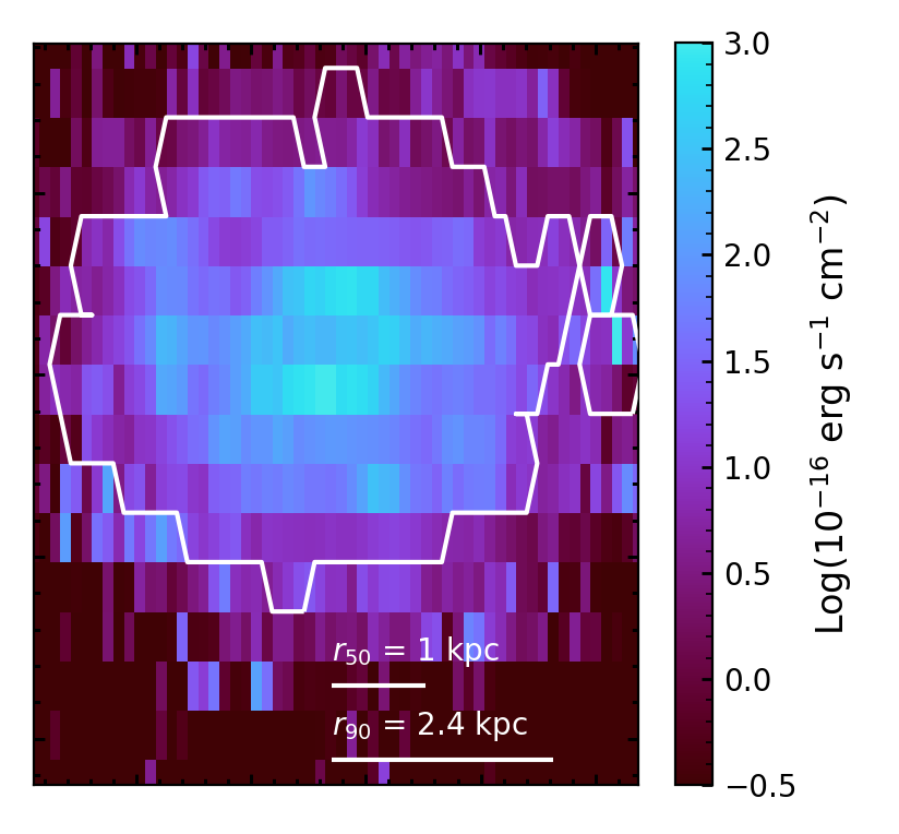
Figure 1: Map of the [OIII] 5007 Å emission line flux from our KCWI data. The white contours show where we have spaxels with a signal-to-noise of greater than 20 per pixel in a 5 Å-wide continuum region blueward of the [OIII] 5007 Å emission line.

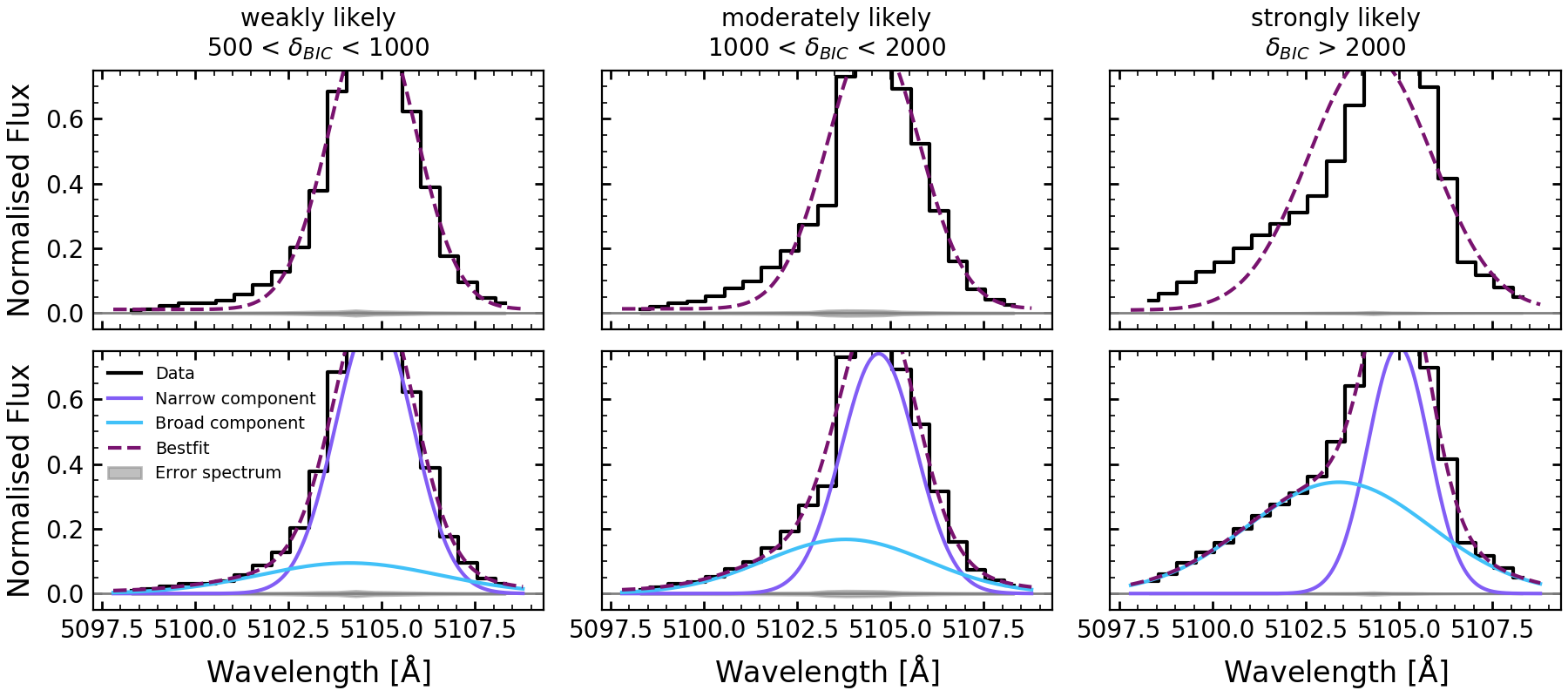
Figure 2: Three examples of fits of the continuum-subtracted [OIII] $\lambda 5007$ emission line made using koffee. The same spaxel is shown in each column with the fit made using a single Gaussian (top row) and the fit made using two Gaussians (bottom row). Data and fits have been normalised to the peak. The grey shaded area indicates the $1\sigma$ error spectrum. The significance level of each double Gaussian fit corresponds to the amount by which the BIC${}_{\rm{double~{}Gaussian}}$ is better than the BIC${}_{\rm{single~{}Gaussian}}$ (see text).

In the case of resolved outflows we do not know a priori which spaxels require multiple Gaussian components and which do not. The simple assumption that all spaxels have an extra Gaussian, and thus an outflow, may lead to specious results. In this work we generate software, koffee, that applies a series of tests to each spaxel to determine if an outflow component is justified.

4.1 Overview of fitting method

We only fit spaxels with a signal-to-noise (S/N) of greater than 20 per pixel in the continuum. This is measured in a region of bandwidth that is $\sim$5 Å wide bluewards of the [OIII] 5007 Å emission line. In Figure 1 we show the [OIII] 5007 Å emission line flux across the KCWI cube. The white contours show where we have spaxels with a S/N $>20$. In our observations of IRAS08 we find S/N $>20$ to galactocentric radii beyond the 90% radius of the optical continuum (6.1″or 2.4 kpc), and therefore are able to represent the outflow activity across the full face of the disk.

An image of the [OIII] 5007 Å line is shown in Fig. 1, with a white contour representing the area in which the continuum exceeds our threshold. The high S/N and spatial resolution of our data is sufficient to identify the star-forming ring as well as other areas of high star formation in the disk. The [OIII] 5007 flux covers a difference of almost 3 orders of magnitude. Typical flux values in the ring are $\sim$250-1000 $\times 10^{-16}~{}\mathrm{erg~{}s}^{-1}~{}\mathrm{cm}^{2}$, where as in the fainter parts of the disk values can be as low as $\sim$3-10 $\times 10^{-16}~{}\mathrm{erg~{}s}^{-1}~{}\mathrm{cm}^{2}$. Under the typical assumption that outflow properties are linked to star formation and the emission line flux traces star formation to first order, the large range in flux values will allow us to detect a range of outflow behaviours. We leave investigation of the impact on our results of varying this S/N cut to future work.

For each spaxel with S/N $>20$, koffee takes a continuum-subtracted emission line, and uses the python package lmfit (Newville et al., 2019) using the default Levenberg-Marquardt least squares method to fit the line twice. First with a single Gaussian,

$$f_{\lambda}=A\ exp\left[-\frac{(\lambda-\lambda_{0})^{2}}{2\sigma^{2}}\right]+c,$$ (1)

secondly with two Gaussians,

$$f_{\lambda}= A_{\rm broad}\ exp\left[-\frac{(\lambda-\lambda_{\rm 0,broad})^{2}}{2\sigma_{\rm broad}^{2}}\right]+$$ (2)

$$A_{\rm narrow}\ exp[-\frac{(\lambda-\lambda_{\rm 0,narrow})^{2}}{2\sigma_{\rm narrow}^{2}}]+c,$$

where $A$ is the amplitude, $\lambda_{0}$ is the central wavelength, $\sigma$ is the standard deviation of the Gaussian, and $c$ is a constant used to account for any continuum remaining after the continuum subtraction. The least squares fit is weighted by the error for each spectrum.

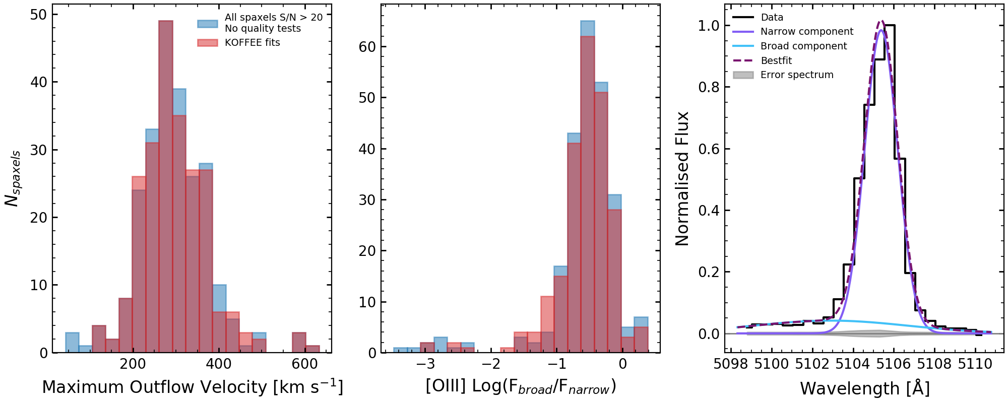
Figure 3: Left and middle panels show the distribution of outflow velocity and [OIII] flux ratio respectively for double Gaussian fitted spaxels. In blue are the results if all 240 spaxels with a signal-to-noise ratio $>20$ in the continuum are assumed to require a broad component. In red are the results for the 230 spaxels which require a double Gaussian fit after undergoing the BIC selection test and the $\chi^{2}_{\rm blue}$ test required by our code (see Eq. 3 and 4). Right is an example of a fit to the [OIII] $\lambda 5007$ emission line for a spaxel which does not require a second Gaussian in the fit, but is assumed to have one if our tests are not applied. Fits such as this over-estimating the number of spaxels where outflows are observable, and may increase scatter in low flux ratio parameter space.

4.2 Fitting Constraints

The following constraints have been placed on the fitted Gaussians: all Gaussians are required to have $\sigma>0.8$Å ($\sim$47 km s^-1). This value is chosen as the minimum dispersion observable with KCWI for our settings. To reduce the number of operations, $\sigma$ has not been convolved with the spectral resolution since the narrow line is unresolved and the broad lines are greater than the instrumental dispersion. All Gaussians are constrained to have $A>0$.

For the double Gaussian fit, the wavelength location of the emission line peak is used to define the expected $\lambda_{\rm 0,narrow}$. From a visual inspection of our data for IRAS08, we find asymmetric emission lines skewed predominately towards the blue (e.g. Fig. 2). The initial guess for $\lambda_{\rm 0,broad}$ is therefore set 0.1Å ($\sim$6 km s^-1) bluewards of $\lambda_{\rm 0,narrow}$. $\lambda_{\rm 0,broad}$ is required to be within 5Å ($\sim$294 km s^-1) of $\lambda_{\rm 0,narrow}$. Initially guesses for $A_{\rm narrow}$ and $A_{\rm broad}$ are given values of 70% and 30% of the emission line peak respectively. The broad Gaussian is required to have $A_{\rm broad}<A_{\rm narrow}$. The initial guess for $\sigma_{\rm narrow}$ is 1.0Å ($\sim$59 km s^-1), and for $\sigma_{\rm broad}$ is 3.5Å ($\sim$206 km s^-1). These initial values were chosen by trial and error.

4.3 BIC Test

We use the Bayesian Information Criterion (BIC) to determine which spaxels are better fit by a double Gaussian. The definition of the BIC is:

$$\mathrm{BIC}=\chi^{2}+N_{\mathrm{variables}}\ln(N)$$ (3)

where $N$ is the number of spectral data points, $N_{\rm variables}$ is the number of variables in the fit (4 for single Gaussians, 7 for double Gaussians), and $\chi^{2}=\sum(f_{\rm{data}}-f_{\rm{model}})^{2}/\sigma^{2}$ is the chi-square statistic calculated from the residuals of the Gaussian fits weighted by the data uncertainty, $\sigma$. A lower BIC value justifies the use of more model parameters to describe data. The BIC provides a quantifiable and automated method of identifying those spaxels that require an outflow component. We note that lmfit’s built-in function for the BIC does not follow this definition, and care should be taken before using their function for fitting purposes.

We define the difference in BIC values,

$$\delta_{BIC}=\mathrm{BIC}_{\rm{single~{}Gaussian}}-\mathrm{BIC}_{\rm{double~{}Gaussian}}.$$ (4)

Typically $\delta_{BIC}=10$ is used to provide evidence against the fit with fewer parameters (Kass & Raftery, 1995; Swinbank et al., 2019; Avery et al., 2021). In this paper We use a more stringent requirement and investigate the impact of this choice of $\delta_{BIC}$ on our results. We first consider all spaxels with $\delta_{BIC}<500$ to not have outflows that are detectable in our data. We then categorise the remaining spaxels, with outflows, according to their respective value of $\delta_{BIC}$ such that: strongly likely, moderately likely or weakly likely to contain an outflow, corresponds to a BIC where $\delta_{BIC}>$ 2000, 1000 and 500 respectively. Example fits for each category are given in Fig. 2. These category boundaries have been chosen after visual inspection of the fits. We note that we find that the minimum $\delta_{BIC}$ is significantly higher than the conventional value described in statistical texts. This is likely due to the known result that even in more typical spiral galaxies emission lines have been shown to be better fit by multiple Gaussian components (Ho et al., 2014). Moroever, imperfect continuum subtraction is a reality in young stellar populations, and in some cases the software may mistake this for a low-flux broad component (e.g. Fig. 3). We, therefore, choose the larger value in order to isolate the broad component that we are assuming to be representative of the outflow. We suggest that before implementing the BIC as an automated method of decision-making in fitting galaxy emission lines, the chosen cutoffs should be rigorously investigated rather than applying values that are not specifically designed for isolating components of galaxy spectra.

We point out those spaxels in the weakly likely category of Fig. 2. According to standard practice these fits have “strong evidence" from their BIC values to be considered outflow spaxels, however many of these spaxels may not be judged as needing an extra component in by-eye analysis.

4.4 $\chi^{2}_{\rm blue}$ Test

We perform a second test intended to specifically determine if the region of the spectrum that may be dominated by outflow is well fit by the model chosen after the BIC test. We calculate $\chi_{\rm blue}^{2}\equiv\Sigma_{i}(f_{\rm model}-f_{\rm data})^{2}/\sigma_{i}^{2}$ in a 4.0Å region blue-ward of $\lambda_{\rm 0,narrow}-\sigma_{\rm narrow}$ for all spaxels using the best fitting model. If $\chi_{\rm blue}^{2}~{}>~{}1.5$, the emission line is refit with a double Gaussian fit using new initial guesses: $\lambda_{\rm 0,broad}$ is shifted 4.0Å ($\sim$240 km s^-1) to shorter wavelength from $\lambda_{\rm 0,narrow}$, and $\sigma_{\rm broad}$ is increased to 8.0Å ($\sim$480 km s^-1). These new initial guesses force the software to explore parameter space including broader outflows with a greater mean offset from the narrow Gaussian. The resulting double Gaussian fit is adopted if it has improved the calculated $\chi_{\rm blue}^{2}$ and has a lower BIC value than the single Gaussian fit.

4.5 Fitting [OIII] and H$\beta$

koffee fits the [OIII] $\lambda 5007$ emission line first, using the results to inform the fit for the H$\beta$ emission line. We do this for multiple reasons. There is a small diminution in the H$\beta$ line due to absorption, which has been removed in the continuum subtraction (see Sec. 3), and this may bias results. Moreover, H$\beta$ is significantly fainter than [OIII] and the S/N is likely to lead to less trustworthy measurements at low surface brightness.

We first assume that the BIC and $\chi^{2}_{\rm blue}$ results on the [OIII] $\lambda 5007$ line apply to H$\beta$. The initial parameter guesses for $\sigma_{\rm narrow}$, $\sigma_{\rm broad}$ and $\lambda_{\rm 0,narrow}-\lambda_{\rm 0,broad}$ are given by the fitted parameters from the [OIII] $\lambda 5007$ results. The parameters are allowed to vary by 1.5Å ($\sim 90~{}\mathrm{km}~{}\mathrm{s}^{-1}$) from those found for [OIII] $\lambda 5007$.

The $\chi^{2}_{\rm blue}$ test is then performed on the double Gaussian H$\beta$ fits. If $\chi^{2}_{\rm blue}>1.5$ for H$\beta$, the emission line is refit with only 0.5Å ($\sim 30~{}\mathrm{km}~{}\mathrm{s}^{-1}$) variation allowed for both parameters. Due to the lower S/N on H$\beta$, we base our refits more heavily on the [OIII] parameters. The resulting double Gaussian fit is adopted if it has improved the calculated $\chi_{\rm blue}^{2}$ and has a lower BIC value than the single Gaussian fit. If $A_{\rm broad}/A_{\rm narrow}>0.9$ we perform a BIC test to decide if the second Gaussian is warranted. If $A_{\rm broad}/A_{\rm narrow}>0.98$ then we assume that only a single Gaussian is observable in H$\beta$. We find that the outflow velocities derived from H$\beta$ are of order 10% lower than those from [OIII].

4.6 Impact of fitting tests on results

In Fig. 3 we show the impact of these tests on our main results for derived outflow properties, comparing the results from koffee and those making the assumption that all spaxels require a double Gaussian fit. Overall, the biases in IRAS08 are not strong, though this may be due to the widespread nature of outflows in this galaxy. Galaxies that are less covered by outflows may have more biases. If we only perform the BIC selection test, 199 out of all 240 spaxels require the double Gaussian fit. When we perform both the BIC selection test and the $\chi^{2}_{\rm blue}$ test, 230 spaxels require the double Gaussian fit.

When all spaxels are assumed to require a double Gaussian fit, there is a population that have low flux ratios (middle panel of Fig. 3). Many of these spaxels do not truly require a second Gaussian to fit the [OIII] $\lambda 5007$ line. An example of such a fit is given in the right-most panel of Fig. 3.

5 Results

5.1 Outflow Velocity

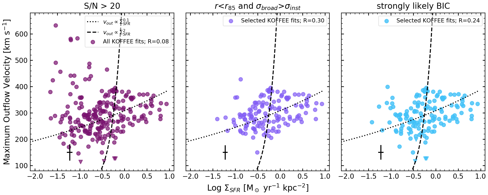
Figure 4: The maximum outflow velocity, $v_{\rm out}$  is plotted against the star formation rate surface density, $\Sigma_{\rm SFR}$, for left: all KCWI spaxels in IRAS08 which require a double Gaussian fit in our data; middle: spaxels requiring a double Gaussian fit which are within $r_{85}$ and have a fitted $\sigma_{\rm broad}$ greater than the instrument dispersion $\sigma_{\rm inst}$; and right: spaxels which are fit with a strongly likely outflow component according to our BIC test. The Pearson’s correlation coefficient, R, is given in the legend of each panel.Two models for the relationship between $v_{\rm out}$ and $\Sigma_{\rm SFR}$ have also been plotted. The dashed line represents a momentum-driven outflow, where the outflow is driven by radiative pressure from young stars ($v_{\rm out}$$\propto$$\Sigma_{\rm SFR}$²; Murray et al., 2011). The dotted line represents an energy-driven outflow, where the outflow is driven by supernova feedback ($v_{\rm out}$$\propto$$\Sigma_{\rm SFR}$^0.1; Chen et al., 2010). Our data most closely resembles the trend expected of an energy-driven outflow.

The relationship between outflow kinematics and the properties of the region launching them has historically been used to discriminate between physical models of the launching mechanism (e.g. Chen et al., 2010; Murray et al., 2011; Newman et al., 2012b). We, therefore, use our results derived from koffee to study such correlations. We find that in IRAS08 this relationship is more consistent with shallow slopes, similar to energy driven winds.

In Figure 4 we show the $\Sigma_{\rm SFR}$ plotted against the maximum outflow velocity, $v_{\rm out}$  defined as

$$v_{\rm out}=|v_{\rm narrow}-v_{\rm broad}|+2\sigma_{\rm broad}$$ (5)

where $v_{\rm narrow}$ and $v_{\rm broad}$ are the velocities at the centre of the narrow and broad Gaussians respectively, and $\sigma_{\rm broad}$ is the standard deviation of the broad Gaussian for the [OIII] $\lambda 5007$ fits which has been corrected for the instrumental velocity dispersion of 0.7 Å or 41.9 km s^-1. In general, these quantities need to be corrected for galaxy inclination, however this is not important in our face-on galaxy. Equation 5 is similar to outflow velocity measurements that have been used in the literature (e.g. Genzel et al., 2011; Davies et al., 2019). We use this definition to make our velocities measured from emission lines more comparable with the maximum velocities measured from absorption line studies. Each data point in Fig. 4 represents a KCWI spaxel in which a double Gaussian fit is required. Spaxel sizes are of order $\sim 100\times 500$ pc. In IRAS08 we find that the average spaxel has a median $v_{\rm out}$ of 288 km s^-1 with root-mean-square scatter of 79 km s^-1. The typical measurement uncertainty on a single spaxel is of order 10-30 km s^-1.

To calculate the $\Sigma_{\rm SFR}$ for each spaxel, we use

$$SFR=\mathrm{C}_{\mathrm{H}\alpha}\frac{L_{\mathrm{H}\alpha}}{L_{\mathrm{H}\beta}}10^{-0.4A_{\mathrm{H}\beta}}L_{\mathrm{H}\beta}$$ (6)

and divide by the KCWI spaxel size. Here C${}_{\mathrm{H}\alpha}=10^{-41.257}$ is the scale parameter (Hao et al., 2011), $L_{\mathrm{H}\alpha}/L_{\mathrm{H}\beta}=2.87$ is the luminosity ratio (Calzetti, 2001), $A_{\mathrm{H}\beta}$ is the extinction and $L_{\mathrm{H}\beta}$ is the observed H$\beta$ luminosity. We have used the observed emission line ratio H$\beta/$H$\gamma$ to correct for extinction in the emission lines (Cardelli et al., 1989; Calzetti, 2001). To calculate $L_{\mathrm{H}\beta}$ for each spaxel we have used the narrow Gaussian fit to H$\beta$ from koffee. The flux contributed by the broad component is interpreted to be outflowing gas, and so is left out of the calculation.

Typical studies do not remove the outflow component from their calculations of the $\Sigma_{\rm SFR}$ from ionised gas emission. Using the combined broad+narrow flux we obtain a total SFR similar to typical estimates (e.g. Östlin et al., 2009). Averaging over all spaxels, we find that taking the outflow into account by removing it causes an average decrease in $\Sigma_{\rm SFR}$ of $\sim$25%. This implies that in star-forming galaxies, such as those at $z>1$, outflows only contribute to a systematic uncertainty in SFR of order $0.15$ dex. This may increase for galaxies with higher $\Sigma_{\rm SFR}$ than our target.

In Fig. 4 we also show two popularly used models for the relationship between $v_{\rm out}$ and $\Sigma_{\rm SFR}$. The dashed line shows the expected relationship if the outflows are momentum-driven ($v_{\rm out}$$\propto$$\Sigma_{\rm SFR}$²; Murray et al., 2011). The dotted line shows the expected relationship if the outflows are energy-driven ($v_{\rm out}$$\propto$$\Sigma_{\rm SFR}$^0.1; Chen et al., 2010).

As discussed above, we do not know a priori which spaxels are appropriate for comparison of outflows to physical models. In Fig. 4 we, therefore, make three separate assumptions on which data is appropriate to compare to the models: all data points with S/N $>20$ in the continuum and at least weakly likely double Gaussian fits (left); those data points within the 85% radius ($r_{85}\sim 4.4$″or 1.7 kpc) and which have resolved dispersions (middle); and those spaxels which have strongly likely double Gaussian fits (see Sec. 4).

In all three panels of Fig. 4 we find that for $\Sigma_{\rm SFR}$ $>0.1~{}$M_⊙ yr^-1 kpc^-2 there is a positive correlation between $\Sigma_{\rm SFR}$ and $v_{\rm out}$. For both the physically selected panel (middle) and the data points selected by stronger BIC fits (right) we find a strong correlation, with Pearson’s coefficients of 0.30 and 0.24 respectively (see Table 1). Moreover, the slope of this correlation is shallow, and thus consistent with typical expectations from energy-driven wind models, where $\Sigma_{\rm SFR}$ $\propto v_{\rm out}^{0.1-0.2}$ (Chen et al., 2010; Li et al., 2017).

In the left-hand panel of Fig. 4, there is an increase in the typical value of $v_{\rm out}$ below a $\Sigma_{\rm SFR}$ of $\sim 0.1~{}$M_⊙ yr^-1 kpc^-2. We find that this increase is due to broad components located at large radius, $r>4.4\arcsec$ ($r_{85}$). The middle panel shows the spaxels remaining after we exclude the 36% of our double Gaussian fitted spaxels located beyond $r_{85}$. We note that 4% of our double Gaussian fitted spaxels have broad Gaussian components that are equivalent to the instrumental dispersion of KCWI for our settings. These are marked as triangles in the left-hand panel. The remaining spaxels (62% of the total) have a median $v_{\rm out}$ of 293 km s^-1 with root-mean-square scatter of 51 km s^-1. Restricting the spaxels included in this way shows that the upturn below $0.1~{}$M_⊙ yr^-1 kpc^-2 is dominated by spaxels at large radius. We note that, as discussed above, IRAS08 is experiencing a distant interaction with a smaller galaxy, and so some mechanism other than star-formation feedback may be driving the kinematics at the edge of the galaxy disk. Excluding high radius points, our data is consistent with the trend expected from the energy-driven model.

Table 1: Statistics for the relationship between $\Sigma_{\rm SFR}$ and $v_{\rm out}$ when considering all of the spaxels with a S/N $>20$ (top section of table, see Fig. 4), only spaxels with S/N $>20$ and $\Sigma_{\rm SFR}$ $>0.1~{}$M_⊙ yr^-1 kpc^-2 (middle section of table), and spaxels with a S/N $>20$ when data is binned to circularised diameters of $\sim 600$ pc (bottom section of table, see Section 5.2 and Fig. 5). Columns are for the categories defined in the panels of Fig. 4. $N$ is the number of spaxels in each category. R is the Pearson’s Correlation Coefficient, and the p-value gives the probability that a similar R-value could be given by uncorrelated systems for all spaxels.

	S/N $>20$ and $\delta_{\rm BIC}>500$	$\delta_{\rm BIC}>500$, $r<r_{85}$ and $\sigma_{\rm broad}>\sigma_{\rm inst}$	Strongly likely BIC $\delta_{\rm BIC}>2000$
$N$	230	137	140
R	0.08	0.30	0.24
p-value	0.24	4x10-4	2x10-3
$\Sigma_{\rm SFR}$ $>0.1~{}$M⊙ yr-1 kpc-2
$N$	186	132	133
R	0.23	0.28	0.30
p-value	2x10-3	1x10-3	5x10-4
Circularised Diameter 0.6 kpc Bins
$N$	89	32	74
R	0.13	0.51	0.17
p-value	0.21	0.003	0.14

In the right-hand panel of Fig. 4, we have restricted our sample to include only spaxels in which are strongly likely to contain an outflow according to our BIC test. This includes 61% of the total spaxels which koffee originally fit with double Gaussians. These spaxels have a median $v_{\rm out}$ of 291 km s^-1 with root-mean-square scatter of 58 km s^-1. The scatter which we find here is on par with the velocity resolution, which may be a contributing factor to the distribution of velocities.

There is an often quoted fiducial threshold value of $0.1~{}$M_⊙ yr^-1 kpc^-2 for entire galaxy measurements, below which outflows are generally not observed (e.g. Heckman, 2002; Veilleux et al., 2005; Heckman et al., 2015). We therefore compare the $\Sigma_{\rm SFR}$$-$$v_{\rm out}$ relationship for all spaxels, and spaxels with $\Sigma_{\rm SFR}$ $>0.1~{}$M_⊙ yr^-1 kpc^-2. Results are given in the top section of Table 1 for all spaxels and the middle section of Table 1 for spaxels with $\Sigma_{\rm SFR}$ $>0.1~{}$M_⊙ yr^-1 kpc^-2. The correlation between $\Sigma_{\rm SFR}$ and $v_{\rm out}$ is strongest for the case in which all $\Sigma_{\rm SFR}$ with physically selected or strongly likely BIC values are included, as indicated by the correlation coefficients. Moreover, as is clear in the right two panels of Fig. 4 there is no evident break in the correlation at this proposed threshold value.

Conversely for more vigorous star formation, Newman et al. (2012b) finds “strong" outflows are restricted to $\Sigma_{\rm SFR}$ $>1~{}$M_⊙ yr^-1 kpc^-2. We find that outflows are widespread with values reaching $\Sigma_{\rm SFR}$ multiple orders of magnitude below this value. We will return to this in a subsequent discussion of mass-loading factor, and also in the Discussion we address the impact on estimates of the covering fraction of outflows in star forming disks.

5.2 Impact of Region Size Averaging on the $\Sigma_{\rm SFR}$ $-v_{\rm out}$ Relationship

We investigate the effect of increasing the spatial sampling scale (i.e. resolution) on the relationship shown in Fig. 4. We note that our intent is to understand the impact of physical sampling scale on the correlation of $v_{\rm out}$ and $\Sigma_{\rm SFR}$, which is subtly different than the blurring due to observed resolution on the sky. Our procedure is similar to what was carried out by Davies et al. (2019) on stacks of regions from different galaxies at larger redshift. We intend a study of spatial resolution in a follow up paper that will include a sample larger than one galaxy.

We binned our spaxels to 13 different region sizes, increasing the sampling iteratively and then refit the relationship. This begins with 0.11$\times$0.53 kpc² (1$\times$1 binning) and increases to $\sim$1.0$\times$1.1 kpc² (9$\times$2 binning). The smallest bin size is the size of a single KCWI spaxel and is designed to sample half the nominal seeing at Keck ($\sim$0.7″or $\sim$0.27 kpc). We represent these rectangular bins on the x-axis of Fig. 6 by the equivalent circularised diameter for each binning scale. Emission lines were shifted to have the same central velocity before being combined to remove line-broadening caused by local variations in the systemic velocity. This shift is done to identify the physical resolution at which the relationship between outflows and galaxy become most correlated. The typical shift increases as the binning size is increased, and ranges on average from 2 km/s when binning 2x1 spaxels (0.2 kpc x 0.5 kpc) to 240 km s^-1 when combining 9x2 spaxels (1 kpc $\times$ 1 kpc). Shifting the emission lines creates a systematic difference between our resolution study and observations of outflows at lower resolution (e.g. Newman et al., 2012b). The typical spatial resolution (in FWHM) of $z\sim 2$ outflow measurements with adaptive-optics data (e.g. Newman et al., 2012b; Genzel et al., 2011) would still be larger than our largest circularised diameter in this study. The binned spaxels were then run through koffee, and $v_{\rm out}$ and $\Sigma_{\rm SFR}$ re-calculated for each bin. Figure 5 shows an example where we have binned the spaxels to a circularised diameter of $\sim 600$ pc. The statistics for this example are given in the bottom section of Table 1.

In Fig. 6 we show how the Pearson and Spearman correlation coefficients for the physically motivated selected spaxels depend on circularised bin diameter. The Pearson correlation coefficient measures the linear correlation between two sets of data. The Spearman correlation coefficient measures nonparametric correlation between two sets of data that are not necessarily normally distributed. If the correlation is close to linear and there are no strong outliers, the Spearman correlation coefficient will be similar to the Pearson correlation coefficient. We find that decreasing the spatial resolution– or increasing the bin size– corresponds with an increase in the correlation coefficients between $\Sigma_{\rm SFR}$ and $v_{\rm out}$. This result can also be seen by comparing the Pearson’s correlation coefficients reported in the top and bottom sections of Table 1.

To explain the above result, we discuss a geometric as well as a timescale motivated argument. We note that these are not mutually exclusive, nor are they the only possible causes.

Using the $\Sigma_{\rm SFR}$ $-$$v_{\rm out}$ correlation makes the implicit assumption that, at our resolution, the outflowing gas is colocated on the sky with the site of the star formation that launched it. However, gas moving at an angle could be observed above an area that is not the launch site, with an unrelated $\Sigma_{\rm SFR}$. We have chosen a target that is near-to face-on. However, the outflows themselves may not occur precisely perpendicular to the face of the disk. This could increase scatter in the $\Sigma_{\rm SFR}$ $-$$v_{\rm out}$ distribution. As the bin size increases, the observed outflowing gas is more likely to be directly linked to the underlying observed $\Sigma_{\rm SFR}$, increasing the correlation between points in the $\Sigma_{\rm SFR}$ $-$$v_{\rm out}$ distribution.

Secondly, during the time between when the outflow was launched and when we observe it, the underlying properties of the star forming region may have changed, causing the $\Sigma_{\rm SFR}$ measured within the bin to change. For example, the supernova driving the winds may mark a decrease in the emission line flux from the HII region over time. This could lead to high $v_{\rm out}$ points being co-located with lower than expected $\Sigma_{\rm SFR}$. Increasing the bin size will then include neighbouring star formation regions. The outflow velocity may better correlate with the “average" local $\Sigma_{\rm SFR}$ in the local region.

It is unclear whether one of these is the dominant effect, or if a combination of the two is causing the increase in correlation between $v_{\rm out}$ and $\Sigma_{\rm SFR}$. More work on larger samples of objects would be informative.

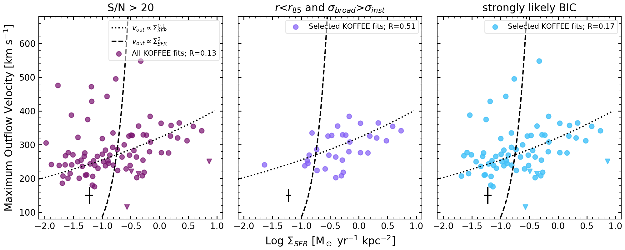
Figure 5: The same as for Figure 4, with our KCWI spaxels binned 5x1 to give 1.45″x1.36″ bins. For IRAS08 at a distance of $\sim$82 Mpc, these are 0.56 kpc x 0.53 kpc bins with an area of 0.3 kpc² and a circularised diameter of $\sim 600$ pc. Increasing the physical size of the bin in which $\Sigma_{\rm SFR}$ and $v_{\rm out}$ are measured clearly creates stronger correlations between these parameters.

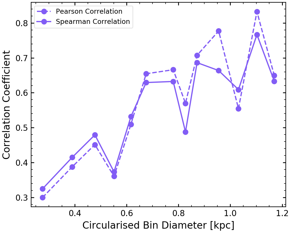
Figure 6: The Pearson (dashed line) and Spearman (solid line) correlation coefficients between the log of the outflow velocity $\log_{10}$($v_{\rm out}$) and the log of the star formation rate surface density $\log_{10}$($\Sigma_{\rm SFR}$) are plotted against the circularised bin diameter. For clarity only the correlation coefficients for the physically motivated selection of points (middle panels of Fig. 4 and Fig. 5) are shown.

5.3 Mass Loading Factor

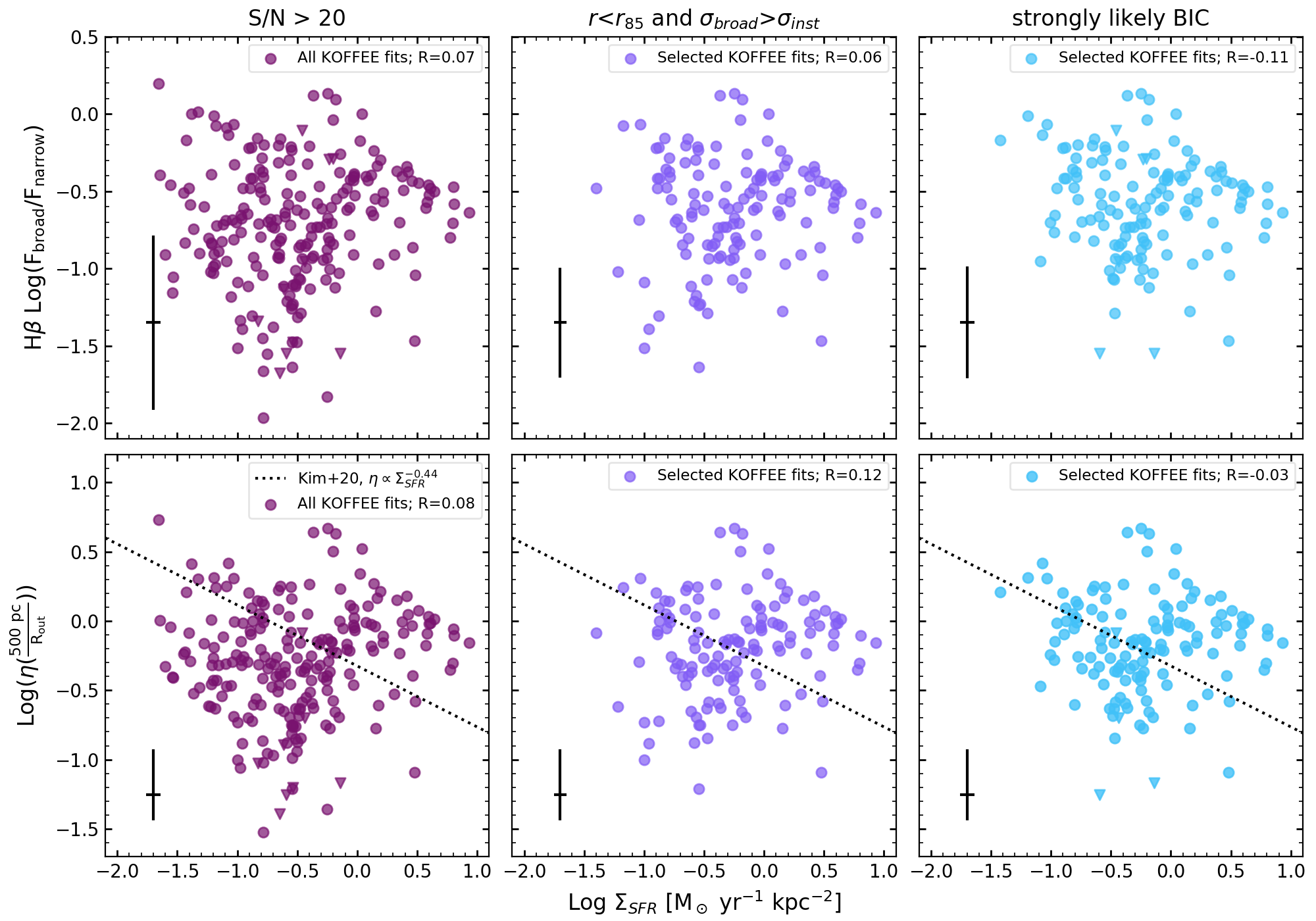
Figure 7: The log of the observed H$\beta$ broad-to-narrow flux ratio F_broad/F_narrow (top row), and the log of the mass loading factor $\eta$ (bottom row) are plotted against star formation rate surface density, $\Sigma_{\rm SFR}$. Panels are defined as in Fig. 4. The Pearson’s correlation coefficient, R, is given in the legend of each panel. A model for the relationship between $\eta$ and $\Sigma_{\rm SFR}$ has also been plotted in each panel of the bottom row (dotted line). The model represents outflows driven by supernova feedback Kim et al. (2020), with an arbitrary scaling factor chosen to match our data. Our data follows a similar trend as the slope found by Kim et al. (2020).

The mass loading factor is the ratio of the mass outflow rate to the star formation rate $\eta=\dot{M}_{\rm out}/\mathrm{SFR}$. Similarly to the kinematics, the mass loading factor is commonly used to test the physical models driving the outflow. It is also used to understand the rate of gas exiting the galaxy, or local region, due to feedback. There are a significant number of uncertainties in deriving $\eta$ which may vary within a galaxy. We consider these in this subsection.

The mass outflow rate is defined as

$$\dot{M}_{\rm out}=\frac{1.36m_{\mathrm{H}}}{\gamma_{\mathrm{H}\beta}n_{e}}\left(\frac{v_{\rm out}}{R_{\rm out}}\right)L_{\rm H\beta,broad}$$ (7)

where $m_{\mathrm{H}}$ is the atomic mass of H, $\gamma_{\mathrm{H}\beta}$ is the H$\beta$ emissivity at $T_{e}=10^{4}$ K ($\gamma_{\mathrm{H}\beta}=1.24\times 10^{-25}~{}\mathrm{erg~{}cm}^{3}~{}\mathrm{s}^{-1}$), $n_{e}$ is the local electron density in the outflow, $v_{\rm out}$ is the maximum outflow velocity which we found in the previous section, $R_{\rm out}$ is the radial extent of the outflow, and $L_{\rm H\beta,broad}$ is the extinction-corrected H$\beta$ luminosity of the broad component. Dividing the mass outflow rate by the SFR defined in Equation 6, the mass loading factor is

$$\eta=\frac{1.36m_{\mathrm{H}}}{\mathrm{C}_{\rm H\alpha}\gamma_{\rm H\beta}n_{e}}10^{0.4A_{\rm H\beta}}\left(\frac{v_{\rm out}}{R_{\rm out}}\right)\frac{L_{\rm H\beta,broad}}{L_{\rm H\beta,narrow}}.$$ (8)

For the electron density in the outflow, we adopt the value of $n_{e}=380~{}\mathrm{cm}^{-3}$, consistent with measurements by Förster Schreiber et al. (2019) and Newman et al. (2012a). The range in likely values of the electron density of outflows is of order $\sim$50-700$\mathrm{cm}^{-3}$, which translates to a systematic uncertainty of order $\sim$1 dex on $\eta$.

A significant source of systematic uncertainty in $\dot{M}_{\rm out}$ is the radial extent of the outflow, $R_{\rm out}$. Along with observational measurement there are intrinsic physical uncertainties in assuming a single scale size for the outflowing gas in a region. The true value of $R_{\rm out}$ may vary point-to-point in a galaxy, and may also vary with time in a specific line-of-sight. For each individual spaxel, the $\dot{M}_{\rm out}$ may be both gas originating from launch sites colocated within that spaxel, and also tangentially launched gas from nearby spaxels. The choice of a single $R_{\rm out}$ for each spaxel therefore depends on our assumptions of the region contributing to the observed outflow.

We have assumed an $R_{\rm out}$ of 500 pc for IRAS08 based on multiple lines of argument from nearby well-studied starbursts and our observations of IRAS08. M82 and NGC 253 are very well-known, edge-on starbursting galaxies, in which the minor axis gas is found to have scale lengths of $400-700$ pc (Leroy et al., 2015) and $200-500$ pc (Krieger et al., 2019; Bolatto et al., 2013) respectively. Similar results are found in NGC 1482 (Veilleux & Rupke, 2002). Alternatively, Chisholm et al. (2016) use photoionisation modelling of absorption features to find that the majority of the outflowing mass from NGC 6090 is within 300 pc of the starburst. More work is direly needed on the extent of outflows in starbursting systems. Nonetheless the work to date suggests that scales of hundreds of parsecs are appropriate. Note due to this uncertainty, we express the mass-loading factor in units of 500 pc/$R_{\rm out}$ to emphasise that this assumption heavily affects this important quantity.

The errorbars for $\eta$ in Fig. 7 include an estimate of the uncertainty in $R_{\rm out}$. For an upper limit, we assume that the maximum value of $R_{\rm out}$ is not larger than the 90% radius of the galaxy (2.4 kpc). For the lower limit, we assume that the bulk of the outflowing material is observed close to its launching site. Simulation work often chooses the scale-height of the disk as a metric. This would be of order $100-200$ pc in a galaxy like IRAS08. For convenience, we use a minimum $R_{\rm out}$ of 350 pc, which is chosen to be similar to the resolution of our KCWI spaxels. This reasoning is similar to that in Davies et al. (2019). The total range in viable assumptions for $R_{\rm out}$ implies a systematic uncertainty on the absolute value of $\eta$ of roughly an order-of-magnitude.

In Figure 7 we plot the H$\beta$ broad-to-narrow flux ratio against $\Sigma_{\rm SFR}$ in the top row, and $\eta$ against $\Sigma_{\rm SFR}$ in the bottom row. The columns represent the same assumptions as in Figure 4. In IRAS08 we find a total mass-loading factor of $\eta\sim 0.81$, by summing the $\dot{M}_{\rm out}$ in all spaxels and dividing by total SFR. However, we strongly urge caution, that because our study is limited to optical ionised gas this number is a low-estimate. We speculate on the full mass-loading factor in the discussion.

From spaxel-to-spaxel the value of $\eta$ varies by 2 orders-of-magnitude. Moreover, there is considerable systematic uncertainty introduced by the assumptions above. Varying the size of $R_{\rm out}$ changes the mass-loading factor to $\sim$0.2 and $\sim$1.2 at the larger and smaller $R_{\rm out}$ bounds respectively.

We note that the inverse correlation in Fig. 7 may be, at least in part, due to a circularity in that $\eta\propto 1/F_{\rm H\beta}$, which is also used to determine $\Sigma_{\rm SFR}$. We therefore investigate what property drives the change in $\eta$. There are three measured quantities that we use to calculate $\eta$. The H$\beta$ broad-to-narrow flux ratio $F_{\rm broad}/F_{\rm narrow}$, and $v_{\rm out}$ from the [OIII] $\lambda 5007$ line, which can be further broken into the velocity difference $v_{\rm diff}=|v_{\rm narrow}-v_{\rm broad}|$ and the outflow velocity dispersion $\sigma_{\rm broad}$. For velocity we find lower correlation coefficients with $\eta$ of 0.10, $-0.33$ and 0.29 for $v_{\rm out}$, $v_{\rm diff}$ and $\sigma_{\rm broad}$ respectively. We have plotted the relationship between H$\beta$ $F_{\rm broad}/F_{\rm narrow}$ and $\Sigma_{\rm SFR}$ in the top row of Fig. 7 for comparison to $\eta$. We see similar behaviour in both $\eta$ and H$\beta$ $F_{\rm broad}/F_{\rm narrow}$. We find that there is a much stronger correlation ($R\sim 0.97$) between H$\beta$ $F_{\rm broad}/F_{\rm narrow}$ and $\eta$ than there is with either of the components of $v_{\rm out}$. We conclude that the main driver of $\eta$ is the observed H$\beta$ $F_{\rm broad}/F_{\rm narrow}$.

In the lower panels of Figure 7 we plot the relationship $\eta~{}\propto$ $\Sigma_{\rm SFR}$^-0.44 from simulation (Kim et al., 2020), in which outflows are driven primarily by energy-driven winds similarly to the dotted line in Fig. 4. Li et al. (2017) similarly find $\eta~{}\propto$ $\Sigma_{\rm SFR}$^-0.43, whereas Creasey et al. (2013) find a slightly steeper relationship of $\eta~{}\propto$ $\Sigma_{\rm SFR}$^-0.74.

In IRAS08, as shown in Fig. 7, we find a roughly constant $\eta$ across $\Sigma_{\rm SFR}$ in all three selection panels of the figure. The median of points in the left panel is $\eta\approx 0.52$ with a root-mean-square scatter of 0.8. This increases to $\eta\approx 0.7$ with a root-mean square scatter of 0.8 in the right panel. The overall trend we find in our data for strongly likely fits (right panel) is consistent with the relationship found by Kim et al. (2020).

Our overall trend in Fig. 7 is different than that measured in galaxies at $z\approx 2$ (Newman et al., 2012b; Davies et al., 2019). Both of those studies find a decrease in $\eta$ for low $\Sigma_{\rm SFR}$. Moreover, we find no evidence of stark change in $\eta$ at $\Sigma_{\rm SFR}$ $=1~{}$M_⊙ yr^-1 kpc^-2, as suggested by Newman et al. (2012b). This could be due to a unique aspect of our target, or alternatively may be due to uncertainties in measurements of the distant galaxies observed with adaptive optics. We note, also, that the SINS data does not reach the low $\Sigma_{\rm SFR}$ values, or the spatial resolution, of our nearby target.

Using NaD absorption line measurements from stacks of MaNGA data, Roberts-Borsani et al. (2020) found a roughly constant relationship between $\eta$ and $\Sigma_{\rm SFR}$ for outflows located inside of twice the half-light radius, over a similar range in $\Sigma_{\rm SFR}$ as ours. They also found an increase in $\eta$ for low $\Sigma_{\rm SFR}$ values at radii larger than 2$\times r_{1/2}$. It is difficult to compare the different tracers of the outflow mass-loading factor. NaD is not covered in our data. A systematic point-to-point comparison of outflows measured with different tracers of gas is direly needed.

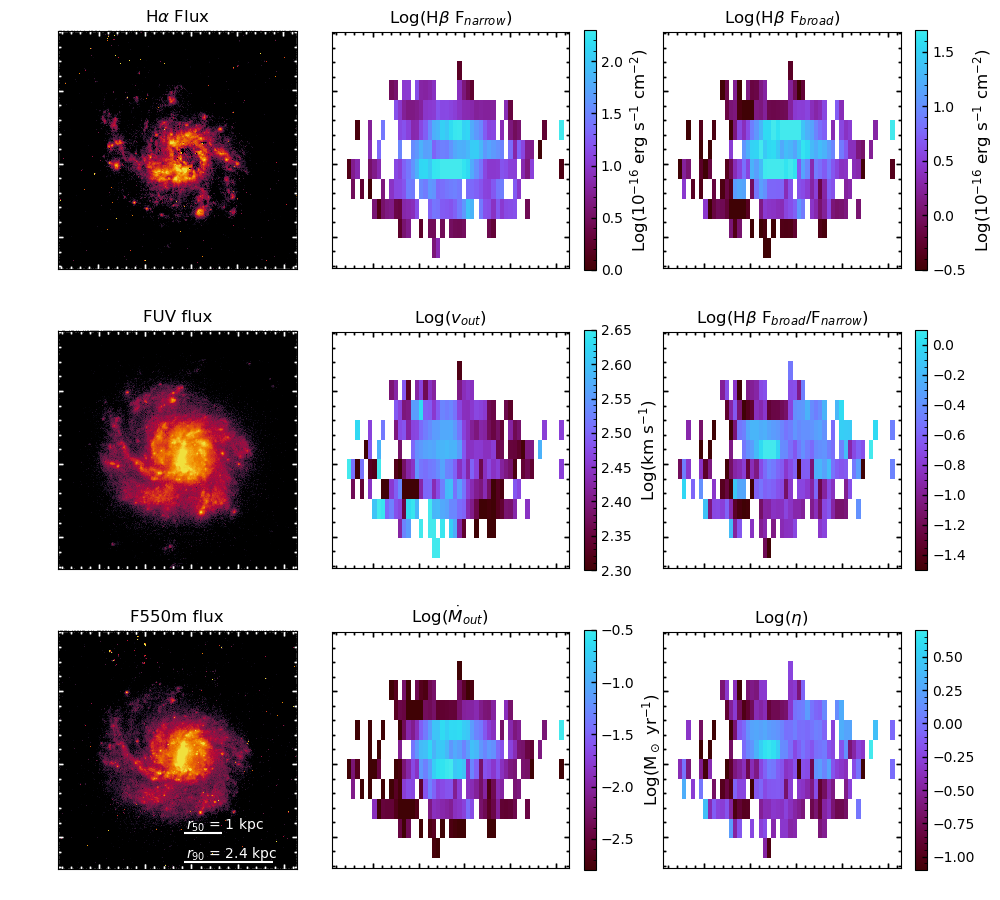
Figure 8: Here we map results from our observations of IRAS08: H$\beta$ narrow line flux from our fitting routine (top row middle), H$\beta$ broad line flux from our fitting routine (top row right), maximum outflow velocity $v_{\rm out}$ calculated using the [OIII] $\lambda 5007$ line (middle row middle), H$\beta$ broad-to-narrow flux ratio F_broad/F_narrow (middle row right), mass outflow rate $\dot{M}_{\rm out}$ (bottom row middle), and mass loading factor $\eta$ (bottom row right). Maps of H$\alpha$, FUV, and F550m flux from $HST$ are also given for comparison, with no extinction correction (left-hand panels of the top, middle and bottom rows respectively). Note that the H$\beta$ emission line has a lower S/N than the [OIII] line, preventing an outflowing component from being resolved in some spaxels. This means that quantities calculated using the H$\beta$ line have 9 fewer spaxels showing in the maps.

5.4 Maps of outflow properties

In Figure 8 we show maps of outflow properties from our KCWI observations and HST images of the ionised gas and starlight. The HST images have not been extinction corrected, however IRAS08 has low extinction ($<0.5$ mag). Our $v_{\rm out}$ is calculated using the fits to the [OIII] $\lambda 5007$ line (Eq. 5). Other than in the $v_{\rm out}$ panel (middle), all panels based on KCWI data use the H$\beta$ flux. Due to the lower signal-to-noise of the H$\beta$ emission line in IRAS08, there are 9 fewer spaxels in which we are able to resolve the outflowing component for these maps. Note that $\dot{M}_{\rm out}$ uses the velocity from [OIII] and luminosity from H$\beta$ (Eq. 7) and that $v_{\rm out}$ from H$\beta$ is consistent with that of [OIII] to $\sim$10%, but [OIII] has higher S/N.

We find that in IRAS08, outflows are ubiquitous inside $r_{50}$ (1 kpc) with 100% of spaxels containing outflows. This decreases at larger radius to 64% of spaxels containing outflows from $r_{50}$ to $r_{90}$ (1 kpc to 2.4 kpc). This trend is most clearly illustrated in the $v_{\rm out}$ panel of Fig. 8. Inside $r_{90}$ (2.4 kpc) 70% of all spaxels contain outflows. A recent survey of MaNGA galaxies with a broad range of SFRs found only 7% contain detectable ionised gas outflows, with only roughly 1 spaxel per galaxy with an outflow (Rodríguez del Pino et al., 2019). It is important to note that the MaNGA data has significantly reduced sensitivity compared to our KCWI data. Nonetheless, our results are consistent with outflows being widespread in disks with high $\Sigma_{\rm SFR}$.

For IRAS08 we calculate a total $\dot{M}_{\rm out}\approx 7.9$ M_⊙ yr^-1. This is an order of magnitude greater than the $\dot{M}_{\rm out}$ calculated by Chisholm et al. (2017) of $\sim$0.33 M_⊙ yr^-1 using UV absorption lines with HST/COS. We note that we sum up a larger area of the galaxy than is included in the 2.5″ diameter ($\sim 1$ kpc) COS pointing used by Chisholm et al. (2017). If we sum up an area of similar size to a COS pointing, we find $\dot{M}_{\rm out}\approx 6.0$ M_⊙ yr^-1. All spaxels included in our total $\dot{M}_{\rm out}$ are shown in the bottom middle panel of Fig. 8 and cover an area with a diameter $\sim 4$ kpc. These spaxels cover 70% of the total galaxy surface area.

The vast majority of the outflowing mass originates from the star forming ring, not from the galaxy centre. If we combine the spaxels containing the galaxy ring, we measure a $\dot{M}_{\rm out}$ that is 60% of the total outflowing mass from the entire galaxy located within 8% of the total galaxy surface area. This has significant implications for the interpretation of single slit observations of outflows. Placing a slit simply on the galaxy centre may not necessarily capture the bulk of the outflowing mass. Parameter correlations with outflow properties for the entire galaxy (e.g. Heckman et al., 2015; Chisholm et al., 2015) may therefore have increased scatter from this effect.

Because the calculation of $\dot{M}_{\rm out}$ depends on multiple observables, we check that this peak in $\eta$ around the galaxy ring is reflected in the observed emission lines. In the top right panel of Fig. 8, we show that total H$\beta$ flux from the broad spectral component is co-located within the region of the strong $\dot{M}_{\rm out}$. We find a similar result with the [OIII] line.

6 Summary and Discussion

We have made resolved measurements of IRAS08 multi-component emission lines using observations from KCWI/Keck. We interpret the broad component as indicative of an outflow. Using a fitting method that incorporates statistical and physically motivated tests, we have measured the kinematics and distribution of outflows across the disk in IRAS08. We have two main results: firstly, we find that our trends of $\Sigma_{\rm SFR}$ vs. $v_{\rm out}$ and $\Sigma_{\rm SFR}$ vs. $\eta$ are both broadly consistent with models of energy-driven winds. Moreover, we find this correlation becomes more robust at spatial scales between 0.6-1 kpc. Secondly, outflows are not limited to the galaxy centre, but are found with varying frequency at all radii within the 90% radius of star light. Indeed, the bulk of outflowing mass is not colocated with the peak of galaxy emission. We discuss the implications of these results in the following subsections.

6.1 Fitting Method: koffee

We develop a method for fitting outflows in galaxies resolved to sub-kpc level. The problem of measuring resolved outflows presents the challenge of both deciding in which spaxels to use the extra component, and determining proper initial choices that facilitate the true $\chi^{2}$ minimum in traditional regression packages. We apply a series of tests to determine whether fitting two Gaussians is justified in each spaxel. Making the simple assumption that all spaxels contain outflows leads to biases in measurements of outflows. The most significant is the presence of a large number of low velocity outflows, and the significant increase in the outflows that have very high broad-to-narrow flux ratios. Not incorporating similar tests for both outflow parameter estimation and the necessity of multiple Gaussian components would lead to a over estimation of physically interpreted quantities like the mass-loading factor.

6.2 Comparison to Theory: Outflow Velocity

It is widely accepted that the relationship between $v_{\rm out}$ and $\Sigma_{\rm SFR}$ provides constraints on the driving mechanisms behind the outflows. Two popular models are energy-driven outflows, where $v_{\rm out}$ $\propto$ $\Sigma_{\rm SFR}$^0.1 (e.g. Chen et al., 2010; Li et al., 2017; Kim et al., 2020; Li & Bryan, 2020) and momentum-driven outflows, where $v_{\rm out}$ $\propto$ $\Sigma_{\rm SFR}$² e.g. Murray et al., 2011; see also discussion in Kornei et al., 2012. Our results from IRAS08 are consistent with shallow powerlaws, as shown in Fig. 4 and Fig. 5. There is currently not a clear consensus in the literature on the exact slope of the $v_{\rm out}$$-$$\Sigma_{\rm SFR}$ relationship when measured for global galaxies. A number of studies do show shallow slopes (e.g. Heckman et al., 2015; Rodríguez del Pino et al., 2019; Roberts-Borsani et al., 2020) alternatively others do not find a robust correlation (e.g. Rubin et al., 2014; Chen et al., 2010). The important distinction between our observations and galaxy integrated studies is that our method removes an implicit correlation with galaxy mass, which is strongly correlated with observed outflow properties (e.g. Chisholm et al., 2015; Heckman et al., 2015). Resolved studies, such as ours, are therefore an important step forward in fully characterising the dependency of outflow kinematics on properties of the underlying stellar population.

Using stacked $\sim$1 kpc spaxels from the SINS sample, Davies et al. (2019) found a steeper relationship than ours, such that $v_{\rm out}$ $\propto$ $\Sigma_{\rm SFR}$^0.3 for ionised gas. They argued that because this result lies between the energy- and momentum-driven models, outflows in their data are driven by a combination of energy and momentum mechanisms. However, comparing our resolved results directly to those from stacked galaxy studies (e.g. Davies et al., 2019; Roberts-Borsani et al., 2020) may be too simplistic. Stacking galaxies may have systematic biases in comparison to individual resolved targets. We do not find that degrading the resolution to $\sim$1 kpc scales results in a different correlation. Indeed, the power-law remains shallow for all sampling scales we probe. Moreover, very different flux sensitivities could lead to differences in returned outflow properties, for example high velocity low mass winds. It is not simple to understand how these would propagate through stacks. We note that if we average our results to make a single galaxy data point, then it does fall within the range of Davies et al. (2019)’s 1-2 kpc-scaled data. Future work with JWST will likely prove informative to resolved outflows at $z>1$.

Overall we find that the $v_{\rm out}$$-$$\Sigma_{\rm SFR}$ relationship in IRAS08 is consistent with those theories and simulations that drive outflows via energy from supernovae, rather than those that drive outflows via momentum from radiation by young stars.

6.3 Comparison to Theory: Mass Loading Factor

Similar to the velocity, the relationship between $\eta$ and $\Sigma_{\rm SFR}$ can place constraints on the driving mechanisms behind the outflows. The mass loading factor, $\eta$, is a measure of how efficiently the outflowing gas is coupled to the energy produced through the star formation process. Values of $\eta~{}\sim~{}1$ indicate that the mass of outflowing gas is comparable to the mass of gas being converted into stars. Low values of $\eta$ indicate that much more gas is converted into stars than is expelled in outflows, meaning that the energy from star formation is inefficiently coupled to the outflowing gas, or the star formation activity is insufficient to drive an outflow.

We note that the total mass of outflows is multiphase in nature (e.g. Fluetsch et al., 2020; Herrera-Camus et al., 2020), and work on local starbursts and spirals suggests that the molecules dominate the outflow mass budget. The total value of $\eta$ in this work, therefore, significantly underestimates the total mass of the outflow. For example, Bolatto et al. (2013) have found $\eta\sim 1-10$ in molecular phase gas in local starbursts with similar $\Sigma_{\rm SFR}$ as our target. In a galaxy at $z\sim 5$ with similar $\Sigma_{\rm SFR}$ to IRAS08, Herrera-Camus et al. (2021) found very high values of $\eta$ in spatially resolved [CII]. Fluetsch et al. (2020) compared ionised gas outflows to those of molecules in 4 galaxies with high SFR/M_star, similar to IRAS08. They found roughly equal $\dot{M}_{\rm out}$ in the phases. This would imply $\eta\sim 2$ in IRAS08. Alternatively Roberts-Borsani (2020) found that ions contribute a much lower fraction by mass, of order $\sim$1% in nearby spirals of significantly lower SFR. This would make the mass-loading factor in IRAS08 very high. We therefore assume a reasonable total $\eta$ for IRAS08 is of order $\eta\sim 2-10$. Work directly comparing resolved outflows in both ions and molecules of starbursts is needed to interpret observations such as ours and those of high-z disks (e.g. Davies et al., 2019).

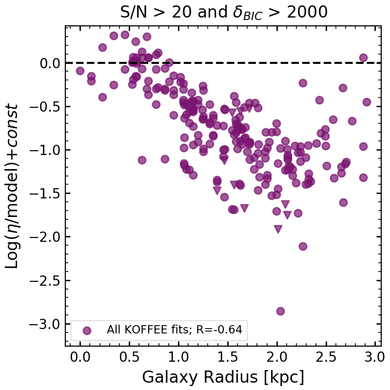
Figure 9: The y-axis shows the mass loading factor $\eta$ divided by the expected values for $\eta$ for their measured $\Sigma_{\rm SFR}$ from the supernovae driven wind model described in Kim et al. (2020), offset to zero at the galaxy centre by a constant. This is the same model which is shown in Fig. 7. The x-axis is the galaxy radius of each spaxel in kiloparsecs. The Pearson’s correlation coefficient, R, is given in the legend. Points above (below) 0.0 indicate the model underestimated (overestimated) the $\eta$ value. We find a strong trend of increasing overestimation of $\eta$ by the model compared to the observed data with increasing galaxy radius.

Our observations of IRAS08 find a slight inverse correlation of $\eta$ with $\Sigma_{\rm SFR}$ for the highly likely outflow fits, and no correlation for the remainder of the data (Fig. 7). Comparing to simulations, our results are consistent with those found by Li et al. (2017) and Kim et al. (2020). Other models incorporating energy-driven winds have also given negative slopes, under typical assumptions (e.g. Creasey et al., 2013).

Our slight inverse correlation of $\eta-$$\Sigma_{\rm SFR}$ is different from most observational studies, though it is difficult to say how these differences may depend on the method. Unlike with velocity, calculating $\eta$ requires normalising by the SFR. This may introduce systematic differences between resolved studies, stacks and global galaxy measurements. A positive correlation between $\eta$ and $\Sigma_{\rm SFR}$ was found for stacks of SINS galaxies (Newman et al., 2012b; Davies et al., 2019) and for SDSS galaxies (Chen et al., 2010).

In Figure 9 we make a more detailed comparison between the $\eta$ in IRAS08 and that predicted by the models from Kim et al. (2020). Note that we have adjusted the values to set $\log(\eta_{data}/\eta_{model})=0$ at the centre of the galaxy, and then consider the relative change. We find that our values of $\eta$ are increasingly lower, with respect to the model, with increasing radius. Using radial stacks of MaNGA data, Roberts-Borsani et al. (2020) found that for fixed $\Sigma_{\rm SFR}$, $\eta$ increased with increasing galaxy radius, in a way that is similar to IRAS08 (see also our Fig. 8). Their results suggest that a property other than star formation processes may be varying $\eta$ across the galaxy disk.

From Eq. 7, the calculation of $\eta$ depends on $v_{\rm out}$, the flux ratio $F_{\rm broad}/F_{\rm narrow}$, and inversely depends on the outflow radius $R_{\rm out}$ and electron density $n_{e}$. Our results for $v_{\rm out}$ agree well with the model for energy-driven outflows (Fig. 4), and thus $v_{\rm out}$ is not likely driving the behaviour in Fig. 9. We note that Kim et al. (2020) used kpc-scale box simulations and may not take into account possible differences in sub-galactic environments. In the following paragraphs we consider possible assumptions for each of the remaining parameters that could lead to our result.

Firstly, a very simple reason could be the available gas in the surrounding region of the galaxy. At the edge of a galaxy the local gas mass surface density is lower. A supernova explosion at the outskirts of the disk might have less gas available to entrain as it moves through the disk. This could then decrease the observed $F_{\rm broad}/F_{\rm narrow}$ without significant changes to the underlying physics.

$R_{\rm out}$ is among the least well constrained quantities in estimating $\eta$. In this work, we assume a constant $R_{\rm out}$ across all spaxels. The true value of $R_{\rm out}$ may, in fact, change from spaxel-to-spaxel across the face of IRAS08. Nonetheless, we could make the ad hoc assumption that $R_{\rm out}$ increases with increasing galactocentric radius. This could, for example, occur if the $R_{\rm out}$ were coupled to local disk thickness, which increases with radius (e.g. García de la Cruz et al., 2021). Alternatively, one could make the ad hoc assumption that large $\Sigma_{\rm SFR}$ generates larger $R_{\rm out}$. It is, however, difficult to understand how $R_{\rm out}$ would vary with $\Sigma_{\rm SFR}$ without also changing $v_{\rm out}$.

Another possibility is that the assumption of a constant $n_{e}$ across the face of the galaxy is incorrect. It seems plausible that more energetic outflows could alter the physical properties of the entrained gas, such as temperature and $n_{e}$. In principle this could be checked with follow up observations with higher spectral resolution in the [OII] doublet or alternatively a separate instrument capable of measuring the [SII] doublet, which is outside of KCWI’s wavelength range. As is discussed in previous works (e.g. Davies et al., 2019), the $n_{e}$ of outflows is poorly constrained, especially in these strong wind systems.

Altogether, our results in IRAS08 for both $v_{\rm out}$$-$$\Sigma_{\rm SFR}$ and $\eta-$$\Sigma_{\rm SFR}$ relations are consistent with models for energy-driven outflows. We note that we have only discussed consistency with the powerlaw slope. For example, the simulations of Kim et al. (2020) have found a similar powerlaw in the outflow velocity, but only produced outflows with velocity of order $\sim$100 km s^-1 at the same $\Sigma_{\rm SFR}$ as our target. Historically, it has been noted that supernova-driven outflows, under standard assumptions, do not produce as high velocity winds as has been observed in starbursting galaxies (Fielding et al., 2018). The precise definition of $v_{\rm out}$ used may introduce systematics at the factor of a few level. An apples-to-apples comparison to mock observations would be useful in this case.

6.4 Implications of the Spatial distribution and Covering fraction of outflows

Determining the mass-outflow rate for an entire galaxy requires estimating the fraction of the star light that is covered by outflows. In large surveys of unresolved galaxies this is almost always an assumed quantity, often with guidance from the residual flux of saturated absorption lines (review Veilleux et al., 2020). Our observations can give guidance on covering fractions of star bursting disks.

Outflows in disk galaxies in our local universe are typically thought to have biconical outflows (e.g. Bland & Tully, 1988; Shopbell & Bland-Hawthorn, 1998), where the base of the outflow is narrowly focused on the centre of the galaxy. However, from our observations of IRAS08 we have found the signature of outflows across the entire galaxy disk. Within $r_{50}$ we find $\sim$100% of the disk has detectable outflows, and $\sim 70$% of the area within $r_{90}$. This is consistent with absorption line measurements from Chisholm et al. (2017) who find $\sim 80\%$ on gas within $r_{50}$ of IRAS08. Our results suggest that disk galaxies with high $\Sigma_{\rm SFR}$ will not have the same distribution of winds as nearby starbursts. If one defines the covering fraction simply as the ratio of the continuum which has associated outflows, our results imply large covering fractions, $C_{f}\approx 0.7-1$, for disk galaxies with high SFR surface density, as is common above $z>0.5$.

In IRAS08, $\dot{M}_{\rm out}$ measurements are heavily concentrated in a small region of the galaxy, corresponding to the star forming ring contained with a radius of $\sim$0.5 kpc of the galaxy centre (Fig. 8). Indeed, 60% of the total outflow mass is colocated with this ring, which only covers 8% of the total area of the star-light within $r_{90}$. If one observed IRAS08 with low spatial resolution the outflow mass might reflect this smaller region. The flux measured from only the ring would therefore make a small difference on the mass outflow rate, but the covering fraction might change by an order-of-magnitude.

There has been debate about whether outflows in starbursting galaxies at high-z are galaxy-wide outflows or whether they are restricted to the high surface brightness clumps of star formation. For example, Bordoloi et al. (2016) placed slits on clumps of a lensed target, and found outflows preferentially located there. Similarly, Newman et al. (2012b) found outflows restricted to high surface brightness clumps. Our results in IRAS08 imply a balanced take. Outflows are found to be wide spread in the disk, but large fractions of that gas may come from small regions. We find no evidence in IRAS08 for a cut-off or reduction in outflow frequency at $\Sigma_{\rm SFR}$ $\sim 0.1$ M_⊙ yr^-1 kpc^-2. One simple way to reconcile our observation with those at $z>1$ would be that the fainter outflows are more challenging to observe with current telescopes. Observations from the upcoming JWST and further in the future ELT are likely to determine if this is the case.

In summary we found that the scaling relationships of outflow properties with the colocated $\Sigma_{\rm SFR}$ is in general consistent with predictions in which outflows are primarily driven by supernovae. However, this is only one target and differences may occur galaxy to galaxy, which must be accounted for. Future work applying our technique to more targets is needed to test these results. We will apply our technique to the face-on targets in the DUVET survey in a future paper.

Data Availability

The DUVET Survey is still in progress. The data underlying this article will be shared on reasonable request to the PI, Deanne Fisher at dfisher@swin.edu.au

References

- Arribas et al. (2014) Arribas S., Colina L., Bellocchi E., Maiolino R., Villar-Martín M., 2014, A&A, 568, A14
- Avery et al. (2021) Avery C. R., et al., 2021, MNRAS,
- Bland & Tully (1988) Bland J., Tully B., 1988, Nature, 334, 43
- Bolatto et al. (2013) Bolatto A. D., et al., 2013, Nature, 499, 450
- Bordoloi et al. (2016) Bordoloi R., Rigby J. R., Tumlinson J., Bayliss M. B., Sharon K., Gladders M. G., Wuyts E., 2016, MNRAS, 458, 1891
- Calzetti (2001) Calzetti D., 2001, PASP, 113, 1449
- Calzetti et al. (2000) Calzetti D., Armus L., Bohlin R. C., Kinney A. L., Koornneef J., Storchi-Bergmann T., 2000, ApJ, 533, 682
- Cannon et al. (2004) Cannon J. M., Skillman E. D., Kunth D., Leitherer C., Mas-Hesse M., Östlin G., Petrosian A., 2004, ApJ, 608, 768
- Cappellari (2017) Cappellari M., 2017, MNRAS, 466, 798
- Cardelli et al. (1989) Cardelli J. A., Clayton G. C., Mathis J. S., 1989, ApJ, 345, 245
- Chen et al. (2010) Chen Y.-M., Tremonti C. A., Heckman T. M., Kauffmann G., Weiner B. J., Brinchmann J., Wang J., 2010, The Astronomical Journal, 140, 445
- Chisholm et al. (2015) Chisholm J., Tremonti C. A., Leitherer C., Chen Y., Wofford A., Lundgren B., 2015, The Astrophysical Journal, 811, 149
- Chisholm et al. (2016) Chisholm J., Tremonti Christy A., Leitherer C., Chen Y., 2016, MNRAS, 463, 541
- Chisholm et al. (2017) Chisholm J., Tremonti C. A., Leitherer C., Chen Y., 2017, Monthly Notices of the Royal Astronomical Society, 469, 4831
- Creasey et al. (2013) Creasey P., Theuns T., Bower R. G., 2013, MNRAS, 429, 1922
- Davies et al. (2019) Davies R. L., et al., 2019, The Astrophysical Journal, 873, 122
- Ferrara & Ricotti (2006) Ferrara A., Ricotti M., 2006, MNRAS, 373, 571
- Fielding et al. (2018) Fielding D., Quataert E., Martizzi D., 2018, Monthly Notices of the Royal Astronomical Society, 481, 3325
- Fisher et al. (2017) Fisher D. B., et al., 2017, MNRAS, 464, 491
- Fisher et al. (2019) Fisher D. B., Bolatto A. D., White H., Glazebrook K., Abraham R. G., Obreschkow D., 2019, The Astrophysical Journal, 870, 46
- Fluetsch et al. (2020) Fluetsch A., et al., 2020, arXiv e-prints, p. arXiv:2006.13232
- Förster Schreiber et al. (2011) Förster Schreiber N. M., et al., 2011, The Messenger, 145, 39
- Förster Schreiber et al. (2019) Förster Schreiber N., et al., 2019, The Astrophysical Journal, 875, 21
- García de la Cruz et al. (2021) García de la Cruz J., Martig M., Minchev I., James P., 2021, MNRAS, 501, 5105
- Genzel et al. (2011) Genzel R., et al., 2011, The Astrophysical Journal, 733, 101
- Girard et al. (2021) Girard M., et al., 2021, ApJ, 909, 12
- González Delgado et al. (1998) González Delgado R. M., Leitherer C., Heckman T., Lowenthal J. D., Ferguson H. C., Robert C., 1998, ApJ, 495, 698
- Hao et al. (2011) Hao C.-N., Kennicutt R. C., Johnson B. D., Calzetti D., Dale D. A., Moustakas J., 2011, ApJ, 741, 124
- Heckman (2002) Heckman T. M., 2002, in Mulchaey J. S., Stocke J. T., eds, Astronomical Society of the Pacific Conference Series Vol. 254, Extragalactic Gas at Low Redshift. p. 292 (arXiv:astro-ph/0107438)
- Heckman & Borthakur (2016) Heckman T. M., Borthakur S., 2016, ApJ, 822, 9
- Heckman et al. (2000) Heckman T. M., Lehnert M. D., Strickland D. K., Armus L., 2000, ApJS, 129, 493
- Heckman et al. (2015) Heckman T. M., Alexandroff R. M., Borthakur S., Overzier R., Leitherer C., 2015, The Astrophysical Journal, 809, 147
- Herrera-Camus et al. (2020) Herrera-Camus R., et al., 2020, A&A, 635, A47
- Herrera-Camus et al. (2021) Herrera-Camus R., et al., 2021, A&A, 649, A31
- Hinshaw et al. (2013) Hinshaw G., et al., 2013, ApJS, 208, 19
- Ho et al. (2014) Ho I. T., et al., 2014, MNRAS, 444, 3894
- Hopkins et al. (2012) Hopkins P. F., Quataert E., Murray N., 2012, MNRAS, 421, 3522
- Hopkins et al. (2014) Hopkins P. F., Kereš D., Oñorbe J., Faucher-Giguère C.-A., Quataert E., Murray N., Bullock J. S., 2014, MNRAS, 445, 581
- Hung et al. (2019) Hung C.-L., et al., 2019, MNRAS, 482, 5125
- Jones et al. (2018) Jones T., Stark D. P., Ellis R. S., 2018, ApJ, 863, 191
- Kass & Raftery (1995) Kass R. E., Raftery A. E., 1995, Journal of the American Statistical Association, 90, 773
- Kim et al. (2013) Kim C.-G., Ostriker E. C., Kim W.-T., 2013, ApJ, 776, 1
- Kim et al. (2020) Kim C.-G., et al., 2020, ApJ, 900, 61
- Kornei et al. (2012) Kornei K. A., Shapley A. E., Martin C. L., Coil A. L., Lotz J. M., Schiminovich D., Bundy K., Noeske K. G., 2012, ApJ, 758, 135
- Krieger et al. (2019) Krieger N., et al., 2019, ApJ, 881, 43
- Krumholz et al. (2018) Krumholz M. R., Burkhart B., Forbes J. C., Crocker R. M., 2018, MNRAS, 477, 2716
- Leitherer et al. (2002) Leitherer C., Li I. H., Calzetti D., Heckman T. M., 2002, ApJS, 140, 303
- Leroy et al. (2015) Leroy A. K., et al., 2015, ApJ, 814, 83
- Li & Bryan (2020) Li M., Bryan G. L., 2020, ApJ, 890, L30
- Li et al. (2017) Li M., Bryan G. L., Ostriker J. P., 2017, ApJ, 841, 101
- López-Sánchez et al. (2006) López-Sánchez Á. R., Esteban C., García-Rojas J., 2006, A&A, 449, 997
- Madau & Dickinson (2014) Madau P., Dickinson M., 2014, ARA&A, 52, 415
- Martin (2005) Martin C. L., 2005, ApJ, 621, 227
- Morrissey et al. (2018) Morrissey P., et al., 2018, ApJ, 864, 93
- Mosleh et al. (2013) Mosleh M., Williams R. J., Franx M., 2013, ApJ, 777, 117
- Murray et al. (2011) Murray N., Ménard B., Thompson T. A., 2011, ApJ, 735, 66
- Nelson et al. (2019) Nelson D., et al., 2019, MNRAS, 490, 3234
- Newman et al. (2012a) Newman S. F., et al., 2012a, The Astrophysical Journal, 752, 111
- Newman et al. (2012b) Newman S. F., et al., 2012b, The Astrophysical Journal, 761, 43
- Newville et al. (2019) Newville M., et al., 2019, lmfit/lmfit-py 0.9.14, doi:10.5281/zenodo.3381550
- Oppenheimer & Davé (2006) Oppenheimer B. D., Davé R., 2006, MNRAS, 373, 1265
- Östlin et al. (2009) Östlin G., Hayes M., Kunth D., Mas-Hesse J. M., Leitherer C., Petrosian A., Atek H., 2009, AJ, 138, 923
- Ostriker et al. (2010) Ostriker E. C., McKee C. F., Leroy A. K., 2010, The Astrophysical Journal, 721, 975
- Otí-Floranes et al. (2014) Otí-Floranes H., Mas-Hesse J. M., Jiménez-Bailón E., Schaerer D., Hayes M., Östlin G., Atek H., Kunth D., 2014, A&A, 566, A38
- Roberts-Borsani (2020) Roberts-Borsani G. W., 2020, MNRAS, 494, 4266
- Roberts-Borsani et al. (2020) Roberts-Borsani G. W., Saintonge A., Masters K. L., Stark D. V., 2020, MNRAS,
- Rodríguez del Pino et al. (2019) Rodríguez del Pino B., Arribas S., Piqueras López J., Villar-Martín M., Colina L., 2019, MNRAS, 486, 344
- Rubin et al. (2014) Rubin K. H. R., Prochaska J. X., Koo D. C., Phillips A. C., Martin C. L., Winstrom L. O., 2014, ApJ, 794, 156
- Rupke et al. (2005) Rupke D. S., Veilleux S., Sanders D. B., 2005, ApJS, 160, 115
- Saintonge et al. (2017) Saintonge A., et al., 2017, ApJS, 233, 22
- Shetty & Ostriker (2012) Shetty R., Ostriker E. C., 2012, ApJ, 754, 2
- Shopbell & Bland-Hawthorn (1998) Shopbell P. L., Bland-Hawthorn J., 1998, ApJ, 493, 129
- Springel & Hernquist (2003) Springel V., Hernquist L., 2003, MNRAS, 339, 289
- Stanway & Eldridge (2018) Stanway E. R., Eldridge J. J., 2018, MNRAS, 479, 75
- Swinbank et al. (2019) Swinbank A. M., et al., 2019, MNRAS, 487, 381
- Tacconi et al. (2018) Tacconi L. J., et al., 2018, ApJ, 853, 179
- Tumlinson et al. (2017) Tumlinson J., Peeples M. S., Werk J. K., 2017, ARA&A, 55, 389
- Übler et al. (2019) Übler H., et al., 2019, ApJ, 880, 48
- Veilleux & Rupke (2002) Veilleux S., Rupke D. S., 2002, ApJ, 565, L63
- Veilleux et al. (2005) Veilleux S., Cecil G., Bland-Hawthorn J., 2005, ARA&A, 43, 769
- Veilleux et al. (2020) Veilleux S., Maiolino R., Bolatto A. D., Aalto S., 2020, A&ARv, 28, 2
- Weiner et al. (2009) Weiner B. J., et al., 2009, The Astrophysical Journal, 692, 187
- Wilson et al. (2019) Wilson C. D., Elmegreen B. G., Bemis A., Brunetti N., 2019, ApJ, 882, 5
- Wisnioski et al. (2015) Wisnioski E., et al., 2015, ApJ, 799, 209