The LPM Effect in sequential bremsstrahlung: $1/N_{\rm c}^{2}$ corrections

Abstract

An important question concerning in-medium high-energy parton showers in a quark-gluon plasma or other QCD medium is whether consecutive splittings of the partons in a given shower can be treated as quantum mechanically independent, or whether the formation times for two consecutive splittings instead have significant overlap. Various previous calculations of the effect of overlapping formation times have either (i) restricted attention to a soft bremsstrahlung limit, or else (ii) used the large-$N_{\rm c}$ limit (where $N_{\rm c}{=}3$ is the number of quark colors). In this paper, we make a first study of the accuracy of the large-$N_{\rm c}$ limit used by those calculations of overlap effects that avoid a soft bremsstrahlung approximation. Specifically, we calculate the $1/N_{\rm c}^{2}$ correction to previous $N_{\rm c}{=}\infty$ results for overlap $g\to gg\to ggg$ of two consecutive gluon splittings $g\to gg$. At order $1/N_{\rm c}^{2}$, there is interesting and non-trivial color dynamics that must be accounted for during the overlap of the formation times.

1 Introduction

Consider a high-energy gluon showering as it traverses a QCD medium, such as a quark-gluon plasma, via splitting processes such as gluon bremsstrahlung $g\to gg$. At high energy, the formation time for a bremsstrahlung gluon becomes large and encompasses multiple scatterings with the medium, so that one must take into account the Landau-Pomeranchuk-Migdal (LPM) effect LP1 ; LP2 ; Migdal ; BDMPS1 ; BDMPS2 ; BDMPS3 ; Zakharov1 ; Zakharov2 ; Zakharov3 . It is possible for two consecutive splittings in the shower to have overlapping formations times. The corrections to an in-medium parton shower due to overlapping formation times are formally suppressed by a power of $\alpha_{\rm s}$, and it has been of interest for many years to figure out exactly how significant such corrections are.

Such corrections were first analyzed in refs. Iancu ; Blaizot ; Wu for the case where one of the two overlapping splittings is relatively soft (with various other simplifying assumptions we will review later). Subsequently, the program of refs. 2brem ; seq ; dimreg ; QEDnf ; qedNfstop ; qcd has been working toward analysis of the more general case where neither splitting is necessarily soft. However, the analysis of this more general case has used the large-$N_{\rm c}$ approximation. The formalism for treating $N_{\rm c}{=}3$ is known in principle color but may be challenging to implement numerically.

We’d like to know whether or not the $N_{\rm c}{=}\infty$ overlapping formation-time calculations in the literature are a reasonable or poor approximation to the physical case of $N_{\rm c}{=}3$. In this paper, we investigate that question by calculating $1/N_{\rm c}^{2}$ corrections to earlier $N_{\rm c}{=}\infty$ results 2brem ; seq for the effect of overlapping formation times on real double splitting $g\to gg\to ggg$. Our goal is to see whether those corrections, when extrapolated to $N_{\rm c}{=}3$, are large, small, or comparable to the purely parametric estimate $O(1/N_{\rm c}^{2})\sim 10\%$.

In this paper, other than going beyond the $N_{\rm c}{=}\infty$ approximation, we will make the same sort of simplifying assumptions and approximations as in the earlier work of refs. 2brem ; seq ; dimreg ; QEDnf ; qedNfstop ; qcd . We will assume that the medium is static and homogeneous on scales of the formation time and corresponding formation length. We also make the high-energy multiple scattering approximation and so take interactions with the medium to be described by the $\hat{q}$ approximation.

Before proceeding, we should clarify why the first corrections to $N_{\rm c}{=}\infty$ are $O(1/N_{\rm c}^{2})$ instead of $O(1/N_{\rm c})$. If one were to think inclusively about double splitting, then the $g{\to}gq\bar{q}$ (pair production overlapping bremsstrahlung) rate would be an $O(1/N_{\rm c})$ correction to the purely gluonic $g{\to}ggg$ rate because of the relative number of quark colors vs. gluon colors. However, though a calculation of $g{\to}gq\bar{q}$ has not yet appeared in the literature without soft approximations, it may be computed using the same $N_{\rm c}{=}\infty$ techniques that were used to compute $g{\to}ggg$ in refs. 2brem ; seq . So computing $g{\to}gq\bar{q}$ to leading order in the large-$N_{\rm c}$ limit would give no information on the size of corrections to $N_{\rm c}{=}\infty$ methods. Instead, we will focus in this paper exclusively on purely gluonic (overlapping) $g{\to}ggg$. In the $\hat{q}$ approximation, the corrections to $N_{\rm c}{=}\infty$ for the purely gluonic process will be $O(1/N_{\rm c}^{2})$.

Outline

In the next section, we first review the interesting, non-trivial color dynamics that take place for finite $N_{\rm c}$ in calculations of overlapping formation time effects for $g{\to}ggg$. We next discuss the $N_{\rm c}{\to}\infty$ limit and isolate the $1/N_{\rm c}$ and $1/N_{\rm c}^{2}$ corrections to the effective “Hamiltonian” that describes medium-averaged evolution of high-energy gluons involved in the splitting process. In section 3, we start with what are called “sequential diagram” contributions to the $g{\to}ggg$ rate and show how to obtain analytic integral expressions for the $1/N_{\rm c}^{2}$ corrections. The integrals can all be done analytically except for three time integrals, which later will be performed numerically. Section 4 fills in details about low-level $N_{\rm c}{=}\infty$ formulas for applying the $\hat{q}$ approximation to different color combinations of the high-energy gluons involved in the $g{\to}ggg$ process. Section 5 generalizes the approach for sequential diagrams in section 3 to now also cover what are called “crossed diagrams.” That completes the analytic work, and we move on to numerically evaluate the size of our $1/N_{\rm c}^{2}$ corrections in section 6. We also discuss there the relation of our work to earlier work in a different context (relaxing the $N_{\rm c}{\to}\infty$ limit for single splitting rates $g{\to}gg$ that have not been integrated over transverse momentum). Finally, section 7 offers our conclusion.

We should clarify that, for simplicity, we will study $1/N_{\rm c}^{2}$ corrections to only the subset of $g{\to}ggg$ processes that were studied for $N_{\rm c}{=}\infty$ in refs. 2brem ; seq . This leaves out, for example, direct $g{\to}ggg$ through a 4-gluon vertex, as opposed to a sequence of two 3-gluon vertices with overlapping formation times. Such direct 4-gluon processes have been studied in ref. 4point and found to be numerically small for $N_{\rm c}{=}\infty$. Our study also leaves out effective 4-gluon vertices that appear in Light Cone Perturbation Theory from integrating out longitudinally polarized gluons in light-cone gauge. Their contribution even for $N_{\rm c}{=}\infty$ has not yet been completed. (A calculation of their contribution in large-$N_{\rm f}$ QED is included in ref. QEDnf .)

2 Background: Color dynamics

2.1 Warm-up: The BDMPS-Z single splitting rate

Throughout this paper, we draw diagrams for contributions to splitting rates using the conventions of ref. 2brem , which are adapted from Zakharov’s description of splitting rates Zakharov1 ; Zakharov2 ; Zakharov3 . Fig. 1b gives an example for single-splitting (e.g. $g\to gg$) in the medium.

Figure 1: (a) A time-ordered contribution to the rate for single splitting, such as $g\to gg$, with amplitude in blue and conjugate amplitude in red. (b) A single diagram representing this contribution to the rate. In both cases, all lines implicitly interact with the medium. We need not follow particles after the emission has occurred in both the amplitude and conjugate amplitude because we will consider only $p_{\perp}$-integrated rates. (See, for example, section 4.1 of ref. 2brem for a more explicit argument, although applied there to a more complicated diagram.) Nor need we follow them before the first emission because we approximate the initial particle as on-shell. Only one of the two time orderings that contribute to the rate is shown above.

The high-energy particle lines shown in the figure are implicitly interacting with, and scattering from, the gluon fields of the medium, as depicted in fig. 2a, and the rate is implicitly averaged over the randomness of the medium. Such interactions with the medium change the color of each high-energy particle over time. At first, it may seem like calculating the rate would require a complicated analysis of the time dependence of the color of each such particle. Fortunately, this is unnecessary for fig. 2a. To get a flavor for the reason why, consider for a moment the extreme case where the medium itself is weakly-coupled. Then (to leading order in the coupling of the medium) the medium-averaged correlations of interactions with the medium are 2-point correlations, as shown in fig. 2b. Let’s focus on one of these correlations, such as the green line connecting particles 1 and 3 in fig. 2c. Let ${\mathbb{T}}_{n}^{a}$ represent color generators ${\mathbb{T}}^{a}$ (in the appropriate representation) that act on the color state of particle $n$. The interaction of particle 1 with the gluonic field of the medium comes with a factor of $g{\mathbb{T}}_{1}^{a}$. The correlation of a pair of interactions of particles 1 and 3 with the medium then comes with a factor of $(g{\mathbb{T}}_{1}^{a})(g{\mathbb{T}}_{3}^{a})=g^{2}{\mathbb{T}}_{1}\cdot{\mathbb{T}}_{3}$. But this operator is quite trivial because, by color conservation (after medium averaging), the three high-energy particles in fig. 1b must form a color singlet, which means ${\mathbb{T}}_{1}{+}{\mathbb{T}}_{2}{+}{\mathbb{T}}_{3}=0$. So, ${\mathbb{T}}_{1}{+}{\mathbb{T}}_{3}=-{\mathbb{T}}_{2}$ and thus

$${\mathbb{T}}_{1}\cdot{\mathbb{T}}_{3}=\tfrac{1}{2}\bigl{[}({\mathbb{T}}_{1}+{\mathbb{T}}_{3})^{2}-{\mathbb{T}}_{1}^{2}-{\mathbb{T}}_{3}^{2}\bigr{]}=\tfrac{1}{2}({\mathbb{T}}_{2}^{2}-{\mathbb{T}}_{1}^{2}-{\mathbb{T}}_{3}^{2})=\tfrac{1}{2}(C_{2}-C_{1}-C_{3}),$$ (1)

where $C_{i}$ is the quadratic Casimir associated with the color representation of particle $i$. That means that ${\mathbb{T}}_{1}\cdot{\mathbb{T}}_{3}$ reduces to a simple fixed number in this context. (Specifically ${\mathbb{T}}_{1}\cdot{\mathbb{T}}_{3}=-C_{\rm A}/2=-N_{\rm c}/2$ in the case of $g\to gg$.) Because of (1), we do not need to keep track of the dynamics of the individual colors of the three high-energy particles in order to calculate the rate for fig. 1.

Figure 2: (a) $g\to gg$ but now depicting interactions with the medium. Here, each black line ending in a cross represents an interaction of a high-energy particle with the gluon field in the medium. (b) The medium average of those interactions in the case of a weakly-coupled medium. Here the black lines represent 2-point correlations of the medium interactions, which dominate for a weakly-coupled medium. (The 2-point correlations can be written in terms of correlations $\langle A_{\mu}^{a}A_{\nu}^{b}\rangle$ of the background gluon fields present in the medium.) The correlations are drawn as vertical in this time-ordered diagram because, in the high-energy limit, the correlation lengths in the medium are parametrically small compared to the length (time) scale of the high-energy splitting process. [Not shown but also present: short-time 2-point correlations between two medium interactions of the same high-energy particle.] (c) One correlation between particles 1 and 3 is highlighted.

This conclusion can be generalized to strongly-coupled media as well when one describes medium interactions using the $\hat{q}$ approximation. See ref. Vqhat for the argument.

2.2 SU(3) color states for overlapping, double splitting

Fig. 3 shows an example of a contribution to the rate for overlapping double splitting such as $g\to ggg$. In the shaded region, the system has four high-energy particles (three in the amplitude and one in the conjugate amplitude). Again by color conservation, those four particles together must form a color singlet. Unfortunately, unlike the 3-particle case, color neutrality ${\mathbb{T}}_{1}{+}{\mathbb{T}}_{2}{+}{\mathbb{T}}_{3}{+}{\mathbb{T}}_{4}=0$ is not enough to uniquely determine combinations like ${\mathbb{T}}_{i}\cdot{\mathbb{T}}_{j}$ which appear in correlations between high-energy particles’ interactions with the medium. A similar uncertainty arises in more general arguments Vqhat in the context of the $\hat{q}$ approximation.

Figure 3: One diagrammatic contribution 2brem to the rate for double splitting, such as $g\to ggg$.

The source of this ambiguity is that there are many different ways one can make a color singlet out of four gluons (similar to how there are many ways to make a spin singlet out of four spin-1 particles in ordinary quantum mechanics). In SU(3), the color representations of two gluons can be combined as

$$\bm{8}\otimes\bm{8}=\bm{1}_{\rm s}\oplus\bm{8}_{\rm a}\oplus\bm{8}_{\rm s}\oplus\bm{10}_{\rm a}\oplus\overline{\bm{10}}_{\rm a}\oplus\bm{27}_{\rm s},$$ (2)

where the subscripts “$\rm s$” and “$\rm a$” indicate symmetric vs. anti-symmetric color combinations of the two gluons. We could make a color singlet out of four gluons by combining the first two gluons into any color representation $R$ appearing on the right-hand side of (2), then combine the other two gluons into its complex conjugate $\bar{R}$, and then combine the resulting $R$ and $\bar{R}$ into a color singlet. This process is depicted schematically in fig. 4a, labeled “$s$-channel.” These $s$-channel color states form a basis for all 4-gluon color singlet states. Alternatively, one may instead choose a “$t$-channel” or “$u$-channel” basis, as indicated in the figure.

Figure 4: Three ways to form bases for 4-gluon color singlet states. (The terms $s$-channel, etc. are merely evocative here; we are not referring to $2{\leftrightarrow}2$ scattering.)

In this paper, we find it convenient to work in the $u$-channel basis because of particle numbering conventions in earlier papers on overlapping formation times 2brem ; seq . We will label the $u$-basis singlet states as $|R\rangle_{u}$. Our initial basis for discussing 4-gluon singlets is then

$$|{\bm{1}}\rangle_{u},|{\bm{8}}_{\rm aa}\rangle_{u},\,|{\bm{8}}_{\rm as}\rangle_{u},\,|{\bm{8}}_{\rm sa}\rangle_{u},\,|{\bm{8}}_{\rm ss}\rangle_{u},\,|{\bm{10}}\rangle_{u},\,|\overline{\bm{10}}\rangle_{u},\,|{\bm{27}}\rangle_{u}.$$ (3)

For the case where $R={\bm{8}}$, we have to label whether each pair of the four particles formed the ${\bm{8}}$ by a symmetric ($\rm s$) or anti-symmetric (${\rm a}$) combination, as distinguished in (2). As explained in the present context in ref. color , only a 5-dimensional subspace of (3) appears in calculations of overlapping formation times (e.g. fig. 3):

$$|{\bm{1}}\rangle_{u},\,|{\bm{8}}_{\rm aa}\rangle_{u},\,|{\bm{8}}_{\rm ss}\rangle_{u},\,|{\bm{10}}{+}\overline{\bm{10}}\rangle_{u},\,|{\bm{27}}\rangle_{u},$$ (4)

where

$$|{\bm{10}}{+}\overline{\bm{10}}\rangle_{u}\equiv\tfrac{1}{\sqrt{2}}\bigl{(}|{\bm{10}}\rangle_{u}+|\overline{\bm{10}}\rangle_{u}\bigr{)}.$$ (5)

Soon, we will discuss how the color singlet state of the four gluons evolves in the subspace (4) as the gluons travel through the medium. But first, we wish to discuss the generalization from SU(3) to SU($N$).

2.3 SU($N$) color dynamics for overlapping, double splitting

For the sake of compactness, we will refer to the number of quark colors as $N$ rather than $N_{\rm c}$ in the rest of this paper. The generalization of the preceding discussion to $N>3$ is that the tensor product (2) of two gluon colors becomes

$${\rm A}\otimes{\rm A}=\bm{1}_{\rm s}\oplus{\rm A}_{\rm a}\oplus{\rm A}_{\rm s}\oplus``\bm{10}"_{\!\!\rm a}\oplus``\overline{\bm{10}}"_{\!\!\rm a}\oplus``\bm{27}"_{\!\!\rm s}\oplus``\bm{0}"_{\!\!\rm s}\,,$$ (6)

where ${\bm{1}}$ is the singlet representation, ${\rm A}$ is the adjoint representation of SU($N$), and, for example, $``\bm{27}"$ means the SU($N$) representation that generalizes the 27-dimensional representation of SU(3). The scare quotes just mean that, though we quote the size of the representation for $N{=}3$, we really mean the corresponding representation of SU($N$). Note that there is one more term in (6) than in the original SU(3) product (2). This representation $``\bm{0}"$ of SU($N$) smoothly decouples and disappears as one approaches $N\to 3$ from above.

For SU($N$) with $N>3$, there is a 6-dimensional (rather than 5-dimensional) subspace of color singlet states relevant to calculations of overlapping formation times, which is spanned by the basis color ; NSZ6j

$$|{\bm{1}}\rangle_{u},\,|{\rm A}_{\rm aa}\rangle_{u},\,|{\rm A}_{\rm ss}\rangle_{u},\,|``\bm{10}{+}\overline{\bm{10}}"\rangle_{u},\,|``\bm{27}"\rangle_{u},\,|``\bm{0}"\rangle_{u}.$$ (7)

This generalizes (4).

In this paper we will quote some results about 4-particle color singlet states from ref. color , but we have found it convenient to use slightly different overall sign conventions for the definitions of the $u$-channel states (7). The details of the relation between our sign conventions here and those of ref. color may be found in appendix A.1.

In Zakharov’s version of the BDMPS-Z calculation of single splitting rates, the problem is recast as two-dimensional quantum mechanics (in the transverse plane) with an imaginary-valued “potential energy” $V$. Ref. 2brem extended this picture, in the large-$N$ limit, to calculations of overlap effects in double splitting, such as the contribution to the rate represented by fig. 3. The 4-gluon potential needed to treat the shaded region of fig. 3 for finite $N$ was worked out in ref. color for the $\hat{q}$ approximation. The resulting 2-dimensional Hamiltonian for the 4-gluon evolution in the shaded region of fig. 3 was found to be

$$\underline{H}=\frac{P_{41}^{2}}{2x_{4}x_{1}(x_{4}{+}x_{1})E}+\frac{P_{23}^{2}}{2x_{2}x_{3}(x_{2}{+}x_{3})E}+\underline{V}({\bm{C}}_{41},{\bm{C}}_{23})$$ (8a)

with potential

$$\underline{V}({\bm{C}}_{41},{\bm{C}}_{23})=-\tfrac{i}{4}\hat{q}_{\rm A}\Bigl{\{}(x_{4}^{2}+2x_{4}x_{1}\underline{S}_{u}+x_{1}^{2})C_{41}^{2}+(x_{2}^{2}+2x_{2}x_{3}\underline{S}_{u}+x_{3}^{2})C_{23}^{2}\\ +2\bigl{[}\tfrac{1}{2}(x_{4}-x_{1})(x_{2}-x_{3})(\underline{S}_{u}-1)-(x_{4}+x_{1})(x_{2}+x_{3})\underline{T}_{u}\bigr{]}{\bm{C}}_{41}\cdot{\bm{C}}_{23}\Bigr{\}}.$$ (8b)

Above, symmetries have been used to reduce the 4-gluon quantum mechanics problem with transverse positions $({\bm{b}}_{1},{\bm{b}}_{2},{\bm{b}}_{3},{\bm{b}}_{4})$ to an effective 2-particle quantum mechanics problem 2brem ; seq written in terms of $({\bm{C}}_{41},{\bm{C}}_{23})$ with ${\bm{C}}_{ij}\equiv({\bm{b}}_{i}{-}{\bm{b}}_{j})/(x_{i}{+}x_{j})$. The ${\bm{P}}_{ij}$ are the canonical momenta conjugate to the ${\bm{C}}_{ij}$, and $E$ is the energy of the initial particle in the double-splitting process. The $x_{i}$ represent the longitudinal momentum fractions of the four gluons. The underlined quantities in (8) represent $6\times 6$ matrices (for $N>3$) that act on the 6-dimensional space of relevant 4-gluon color singlet states. The matrices $\underline{S}_{u}$ and $\underline{T}_{u}$ encode results for the action of ${\mathbb{T}}_{i}\cdot{\mathbb{T}}_{j}$ on this space in the $u$-channel basis (7), encoded as

$$\underline{{\mathbb{T}}}_{4}\cdot\underline{{\mathbb{T}}}_{1}=-C_{\rm A}\underline{S}_{u}\,,\qquad\underline{{\mathbb{T}}}_{4}\cdot\underline{{\mathbb{T}}}_{2}=C_{\rm A}\bigl{[}\tfrac{1}{2}(\underline{S}_{u}-\underline{\mathds{1}})-\underline{T}_{u}\bigr{]}\,,\qquad\underline{{\mathbb{T}}}_{4}\cdot\underline{{\mathbb{T}}}_{3}=C_{\rm A}\bigl{[}\tfrac{1}{2}(\underline{S}_{u}-\underline{\mathds{1}})+\underline{T}_{u}\bigr{]}$$ (9)

with

$$\underline{S}_{u}\equiv\left(\begin{array}[]{cccccc}~{}1&&&&&\\ &~{}\tfrac{1}{2}&&&&\\ &&~{}\tfrac{1}{2}&&&\\ &&&~{}0&&\\ &&&&-\tfrac{1}{N}&\\ &&&&&\tfrac{1}{N}\end{array}\right)$$ (10a)

and

$$\underline{T}_{u}\equiv\left(\begin{array}[]{cccccc}0&\tfrac{1}{\sqrt{N^{2}-1}}&0&0&0&0\\ \frac{1}{\sqrt{N^{2}-1}}&0&\tfrac{1}{4}&0&\tfrac{1}{2N}\sqrt{\tfrac{N+3}{N+1}}&\tfrac{1}{2N}\sqrt{\tfrac{N-3}{N-1}}\\ 0&\tfrac{1}{4}&0&\tfrac{1}{\sqrt{2(N^{2}-4)}}&0&0\\ 0&0&\tfrac{1}{\sqrt{2(N^{2}-4)}}&0&\tau_{+}&\tau_{-}\\ 0&\tfrac{1}{2N}\sqrt{\tfrac{N+3}{N+1}}&0&\tau_{+}&0&0\\ 0&\tfrac{1}{2N}\sqrt{\tfrac{N-3}{N-1}}&0&\tau_{-}&0&0\\ \end{array}\right),$$ (10b)

where

$$\tau_{\pm}\equiv\tfrac{1}{2N}\sqrt{\tfrac{(N\mp 2)(N\pm 1)(N\pm 3)}{2(N\pm 2)}}.$$ (11)

In this paper, we will need to solve for the 4-gluon evolution of the Hamiltonian (8) in perturbation theory in $1/N$ about the $N{=}\infty$ limit.

2.4 $N{=}\infty$ limit

In the $N{\to}\infty$ limit, (10) becomes

$$\underline{S}_{u}\to\left(\begin{array}[]{cccccc}~{}1&&&&&\\ &~{}\tfrac{1}{2}&&&&\\ &&~{}\tfrac{1}{2}&&&\\ &&&~{}0&&\\ &&&&~{}0&\\ &&&&&~{}0\end{array}\right),\qquad\underline{T}_{u}\to\left(\begin{array}[]{cccccc}0&&&&&\\ &0&~{}\tfrac{1}{4}&&&\\ &~{}\tfrac{1}{4}&0&&&\\ &&&0&\tfrac{1}{2\sqrt{2}}&\tfrac{1}{2\sqrt{2}}\\ &&&\tfrac{1}{2\sqrt{2}}&0&0\\ &&&\tfrac{1}{2\sqrt{2}}&0&0\end{array}\right)\quad\mbox{in basis}\quad\begin{array}[]{l}|{\bm{1}}\rangle_{u}\\ |{\rm A}_{\rm aa}\rangle_{u}\\ |{\rm A}_{\rm ss}\rangle_{u}\\ |``{\bm{10}}{+}\overline{\bm{10}}"\rangle_{u}\\ |``\bm{27}"\rangle_{u}\\ |``\bm{0}"\rangle_{u}\,.\end{array}$$ (12)

Unlike the case of finite $N$, the matrices $\underline{S}_{u}$ and $\underline{T}_{u}$ commute for $N=\infty$. It is therefore possible to find a new basis that simultaneously diagonalizes both matrices:

$$|1\rangle \equiv|{\bm{1}}\rangle_{u}\,,$$

$$|{\rm A}_{+}\rangle \equiv\tfrac{1}{\sqrt{2}}|{\rm A}_{\rm aa}\rangle_{u}+\tfrac{1}{\sqrt{2}}|{\rm A}_{\rm ss}\rangle_{u}\,,$$

$$|{\rm A}_{-}\rangle \equiv\tfrac{1}{\sqrt{2}}|{\rm A}_{\rm aa}\rangle_{u}-\tfrac{1}{\sqrt{2}}|{\rm A}_{\rm ss}\rangle_{u}\,,$$

$$|{\rm A}^{\!\times}\rangle \equiv\tfrac{1}{\sqrt{2}}|``\bm{27}"\rangle_{u}-\tfrac{1}{\sqrt{2}}|``\bm{0}"\rangle_{u}\,,$$

$$|1^{\times}_{+}\rangle \equiv\tfrac{1}{2}|``\bm{27}"\rangle_{u}+\tfrac{1}{2}|``\bm{0}"\rangle_{u}+\tfrac{1}{\sqrt{2}}|``{\bm{10}}{+}\overline{\bm{10}}"\rangle_{u}\,,$$

$$|1^{\times}_{-}\rangle \equiv\tfrac{1}{2}|``\bm{27}"\rangle_{u}+\tfrac{1}{2}|``\bm{0}"\rangle_{u}-\tfrac{1}{\sqrt{2}}|``{\bm{10}}{+}\overline{\bm{10}}"\rangle_{u}\,,$$ (13)

in terms of which the $N{=}\infty$ limits (12) become

$$\underline{S}^{N=\infty}\equiv\left(\begin{array}[]{cccccc}~{}1&&&&&\\ &~{}\tfrac{1}{2}&&&&\\ &&~{}\tfrac{1}{2}&&&\\ &&&~{}0&&\\ &&&&~{}0&\\ &&&&&~{}0\end{array}\right),\qquad\underline{T}^{N=\infty}\equiv\left(\begin{array}[]{cccccc}~{}0&&&&&\\ &~{}\tfrac{1}{4}&&&&\\ &&-\tfrac{1}{4}&&&\\ &&&~{}0&&\\ &&&&~{}\tfrac{1}{2}&\\ &&&&&-\tfrac{1}{2}\end{array}\right)\quad\mbox{in basis}\quad\begin{array}[]{l}|1\rangle\\ |{\rm A}_{+}\rangle\\ |{\rm A}_{-}\rangle\\ |{\rm A}^{\!\times}\rangle\\ |1^{\times}_{+}\rangle\\ |1^{\times}_{-}\rangle\,.\end{array}$$ (14)

We will explain our naming convention for the basis states (13) shortly. We have dropped the subscript $u$ on $\underline{S}^{N=\infty}$ and $\underline{T}^{N=\infty}$ just to keep our notation from becoming too cluttered.

Because $\underline{S}^{N=\infty}$ and $\underline{T}^{N=\infty}$ are both diagonal, the potential (8b), and so the Hamiltonian, does not mix the states (13) for $N{=}\infty$. Each of these states propagates independently for $N{=}\infty$, with non-matrix potentials given by using the corresponding eigenvalues from (14) in place of the matrices $\underline{S}_{u}$ and $\underline{T}_{u}$ in (8b). We will only encounter transitions between these color singlet states when we later investigate the $O(1/N)$ perturbations to $\underline{S}^{N=\infty}$ and $\underline{T}^{N=\infty}$.

The motivation for the names $|1\rangle$ and $|{\rm A}_{\pm}\rangle$ in (13) should be clear enough. One may use the conversion matrices between bases given in appendix A.1 to see that the state $|{\rm A}^{\!\times}\rangle$ defined in terms of $u$-channel color singlet states is equivalent, in the limit $N\to\infty$, to the combination $\bigl{(}|{\rm A}_{\rm aa}\rangle_{s}+|{\rm A}_{\rm ss}\rangle_{s}\bigr{)}/\sqrt{2}$ of $s$-channel basis states. Similarly, the state $|1^{\times}_{-}\rangle$ is equivalent to the $s$-channel basis state $|1\rangle_{s}$, and $|1^{\times}_{+}\rangle$ is equivalent to the $t$-channel basis state $|1\rangle_{t}$. So we may think of the cross “$\times$” in the notation ${\rm A}^{\!\times}$ or $1^{\times}_{\pm}$ as meaning that, for $N=\infty$, the state involves the representation $R={\rm A}$ or $R=1$ in a cross-channel different from our usual $u$-channel representation.

Later we will also use the definitions (13) of basis states when analyzing large but finite $N$. In that case the equivalences just discussed (and so the motivation for the notation) are not exactly correct. So, for $N<\infty$, one may also interpret the cross $\times$ in the colloquial sense of “crossed out”: a warning that the motivation for the notation is no longer precise for those states.

2.5 An aside: Diagrammatic interpretation of basis states for $N=\infty$

We make a brief detour to present another way to characterize the basis (13) for $N=\infty$. This alternative characterization can offer insight and will be used for some detailed arguments in section 4.2, but is not strictly necessary for most of our calculation.

Refs. 2brem ; seq discuss drawing time-ordered diagrams, such as fig. 3 and others on the surface of a cylinder, where time runs along the length of the cylinder. The large-$N$ requirement that $N{=}\infty$ diagrams be “planar” tHooft can be translated to say that no lines should cross on the surface of the cylinder. So, for instance, fig. 3 can be drawn on the cylinder as in fig. 5, where we have numbered the lines during the 4-particle part of the evolution according to the convention of ref. 2brem , which for this diagram corresponds to identifying the longitudinal momentum fractions of the gluons as $(x_{1},x_{2},x_{3},x_{4})=(-1,y,1{-}x{-}y,x)$. Correlation lines, such as the black lines drawn in fig. 2b (and also higher-point correlations), must also be part of the “planar” diagram and so must lie along the surface of the cylinder without crossing any other lines. As a result, for $N{=}\infty$, there can only be correlations between high-energy particles that are neighbors of each other as one goes around the circumference of the cylinder. So, during the 4-gluon phase of the time evolution in fig. 5, the medium interactions of particle 1 can be correlated with those of particles 2 and 4 but not with particle 3. We will indicate this particular sequence as $(1234)$. Any cyclic permutation, such as $(2341)$, would be an equivalent designation, and so would the reverse order $(4321)$ or its cyclic permutations. All that matters for discussing the interactions among the particles in large $N$ is which of the four high-energy gluons are neighbors.

Figure 5: Fig. 3 drawn on a cylinder. Here, solid lines indicate lines drawn on the front of the cylinder, and dashed lines indicate lines wrapping around the back.

With this notation the color singlet states (13) may be identified as (see appendix A.2)

$$|{\rm A}_{+}\rangle\to(1324),~{}~{}\qquad|{\rm A}_{-}\rangle \to(1234),\qquad~{}~{}|{\rm A}^{\!\times}\rangle\to(1243),$$

$$|1\rangle\to(41)(23),\qquad|1^{\times}_{+}\rangle \to(13)(24),\qquad|1^{\times}_{-}\rangle\to(12)(34)$$ (15)

when $N=\infty$. Above, the notation $(ij)(kl)$ means that particles $i$ and $j$ are contracted into a color singlet and that particles $k$ and $l$ are also contracted into a color singlet.

In terms of the cylinder picture of fig. 5, representing states like $(ij)(kl)$ requires two separate cylinders: one for each singlet pair. This is a useful convention because it corresponds naturally to the large-$N$ topological principle that diagrams requiring handles are suppressed. Specifically, as a preview of what we will see later, fig. 6 shows one type of $1/N^{2}$ correction to fig. 5. As time progresses during the 4-gluon part of the evolution, there is a $1/N$ suppressed transition from the $(1234)$ color singlet state to the $(12)(34)$ color singlet state, and then later another such transition to the $(1243)$ color singlet state. In our notation (13), that’s $|{\rm A}_{-}\rangle\to|1^{\times}_{-}\rangle\to|{\rm A}^{\!\times}\rangle$, where each transition will be due to $1/N$ corrections to the Hamiltonian. Some examples of (2-point) correlations of medium interactions are shown by the black lines. In the language of large $N$ diagrammatics, the resulting diagram (interpreted here to include the medium correlations shown) cannot be drawn as a planar diagram, which is why it is $1/N^{2}$ suppressed. In general, there is a suppression by $1/N^{2}$ for every handle needed to draw a diagram on a surface without crossing lines tHooft .

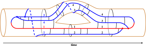
Figure 6: A topological depiction of the $O(1/N^{2})$ transition $(1234)\to(12)(34)\to(1243)$ between $N{=}\infty$ color singlet states during the 4-gluon phase of evolution of fig. 3. The black lines indicate (2-point) examples of correlations of interactions with the medium, which for $N{=}\infty$ are allowed only between neighbors.

2.6 $1/N$ and $1/N^{2}$ corrections to the potential

We can now work out corrections to the $N{=}\infty$ limit by expanding the original Hamiltonian (8) in powers of $1/N$. The dependence on $N$ appears only in the $\underline{S}_{u}$ and $\underline{T}_{u}$ matrices (10), which can be expanded in powers of $1/N$. But we will want to express the result in the basis (13) of states that decouple in the $N{=}\infty$ limit, not the original basis (7) used for presenting $\underline{S}_{u}$ and $\underline{T}_{u}$. After that change of basis,

$$\underline{S}_{u}=\underline{S}^{N=\infty}+\delta\underline{S},\qquad\underline{T}_{u}=\underline{T}^{N=\infty}+\delta\underline{T}+\delta^{2}\underline{T}+O(N^{-3})$$ (16)

with $\underline{S}^{N=\infty}$ and $\underline{T}^{N=\infty}$ as in (14) and

$$\delta\underline{S}=\frac{1}{\sqrt{2}\,N}\begin{pmatrix}~{}0&&&&&\\ &~{}0&&&&\\ &&~{}0&&&\\ &&&0&-1&-1\\ &&&-1&0&0\\ &&&-1&0&0\end{pmatrix},\qquad\delta\underline{T}=\frac{1}{\sqrt{2}\,N}\begin{pmatrix}~{}0&~{}1&~{}1&~{}0&~{}0&~{}0\\ ~{}1&~{}0&~{}0&~{}0&~{}1&~{}0\\ ~{}1&~{}0&~{}0&~{}0&~{}0&~{}1\\ ~{}0&~{}0&~{}0&~{}0&~{}0&~{}0\\ ~{}0&~{}1&~{}0&~{}0&~{}0&~{}0\\ ~{}0&~{}0&~{}1&~{}0&~{}0&~{}0\end{pmatrix},\\ \mbox{and}\quad\delta^{2}\underline{T}=\frac{1}{N^{2}}\begin{pmatrix}~{}0&~{}0&~{}0&~{}0&0&0\\ ~{}0&~{}0&~{}0&~{}\tfrac{1}{2}&0&0\\ ~{}0&~{}0&~{}0&~{}\tfrac{1}{2}&0&0\\ ~{}0&~{}\tfrac{1}{2}&~{}\tfrac{1}{2}&~{}0&0&0\\ ~{}0&~{}0&~{}0&~{}0&-\tfrac{5}{4}&0\\ ~{}0&~{}0&~{}0&~{}0&0&\tfrac{5}{4}\\ \end{pmatrix}\quad\mbox{in basis}\quad\begin{array}[]{l}|1\rangle\\ |{\rm A}_{+}\rangle\\ |{\rm A}_{-}\rangle\\ |{\rm A}^{\!\times}\rangle\\ |1^{\times}_{+}\rangle\\ |1^{\times}_{-}\rangle\,.\end{array}$$ (17)

3 Sequential diagrams

The sample diagram we have been showing so far is called a crossed diagram 2brem because two lines cross when it is drawn as in fig. 3 (as opposed to the drawing in fig. 5 of the same diagram on the cylinder). To study $1/N^{2}$ corrections, it will be simpler to start with a different class of diagrams called sequential diagrams seq , shown in fig. 7. However, only the first diagram $xy\bar{x}\bar{y}$ (and its complex conjugate and permutations) will generate $1/N^{2}$ corrections. That’s because, as discussed earlier, there is no interesting color dynamics for 3-particle propagation, which means that there are no finite-$N$ corrections needed for those propagators provided one uses the value of $\hat{q}$ appropriate for the desired value of $N$. (The same is true of 2-particle propagators.) Only the $xy\bar{x}\bar{y}$ diagram in fig. 7 has a region of 4-particle evolution and so non-trivial color dynamics, denoted by the shaded region in fig. 8.

Figure 7: The above diagrams contributing to double splitting $g{\to}ggg$ are called the “sequential diagrams” in ref. seq . As in refs. 2brem ; seq , the diagrams are individually named ($xy\bar{x}\bar{y}$, etc.) by the time order of the vertices. The relevant permutations referenced above are those permutations of the daughters $x$, $y$, and $z\equiv 1{-}x{-}y$ that create distinct diagrams.

3.1 Set-up and allowed color singlet transitions

We now focus exclusively on the $xy\bar{x}\bar{y}$ diagram. In fig. 8, our numbering of particles in the region of 4-particle evolution follows the same convention as refs. 2brem ; seq . This diagram gives a contribution to the rate for overlapping double splitting $g{\to}ggg$ that is proportional to

$$\int_{t_{\rm x}<t_{\rm y}<t_{\bar{\rm x}}<t_{\bar{\rm y}}}\int_{{\bm{B}}^{\rm y},{\bm{B}}^{\bar{\rm x}}} \nabla^{\bar{n}}_{{\bm{B}}^{\bar{\rm y}}}\langle{\bm{B}}^{\bar{\rm y}},t_{\bar{\rm y}}|{\bm{B}}^{\bar{\rm x}},t_{\bar{\rm x}}\rangle\Bigr{|}_{{\bm{B}}^{\bar{\rm y}}=0}$$

$$\times\nabla^{\bar{m}}_{{\bm{C}}_{41}^{\bar{\rm x}}}\nabla^{n}_{{\bm{C}}_{23}^{\rm y}}\langle{\bm{C}}_{41}^{\bar{\rm x}},{\bm{C}}_{23}^{\bar{\rm x}},t_{\bar{\rm x}}|{\bm{C}}_{41}^{\rm y},{\bm{C}}_{23}^{\rm y},t_{\rm y}\rangle\Bigr{|}_{{\bm{C}}_{41}^{\bar{\rm x}}=0={\bm{C}}_{23}^{\rm y};~{}{\bm{C}}_{23}^{\bar{\rm x}}={\bm{B}}^{\bar{\rm x}};~{}{\bm{C}}_{41}^{\rm y}={\bm{B}}^{\rm y}}$$

$$\times\nabla^{m}_{{\bm{B}}^{\rm x}}\langle{\bm{B}}^{\rm y},t_{\rm y}|{\bm{B}}^{\rm x},t_{\rm x}\rangle\Bigr{|}_{{\bm{B}}^{\rm x}=0}.$$ (18)

Above $(t_{\rm x},t_{\rm y},t_{\bar{\rm x}},t_{\bar{\rm y}})$ are the times of the four vertices in fig. 8 from left (earliest) to right (latest). The factors $\langle{\bm{B}}^{\rm y},t_{\rm y}|{\bm{B}}^{\rm x},t_{\rm x}\rangle$ and $\langle{\bm{B}}^{\bar{\rm y}},t_{\bar{\rm y}}|{\bm{B}}^{\bar{\rm x}},t_{\bar{\rm x}}\rangle$ represent the propagators for the 3-particle evolution respectively before and after the shaded region of the figure. The factor $\langle{\bm{C}}_{41}^{\bar{\rm x}},{\bm{C}}_{23}^{\bar{\rm x}},t_{\bar{\rm x}}|{\bm{C}}_{41}^{\rm y},{\bm{C}}_{23}^{\rm y},t_{\rm y}\rangle$ represents the propagator for the 4-particle evolution inside of the shaded region. There is a gradient ${\bm{\nabla}}$ (corresponding to a factor of transverse momentum) associated with each splitting vertex. We have not shown here other overall factors, including how those gradients are contracted together by helicity-dependent DGLAP splitting functions.

Figure 8: The canonical “sequential” diagram for which finite-$N$ corrections must be calculated.

The only non-trivial corrections to $N{=}\infty$ come from the color dynamics of the 4-particle propagator, which we now write as

$$G({\bm{C}}_{41}^{\bar{\rm x}},{\bm{C}}_{23}^{\bar{\rm x}},t_{\bar{\rm x}};{\bm{C}}_{41}^{\rm y},{\bm{C}}_{23}^{\rm y},t_{\rm y})\equiv\langle{\bm{C}}_{41}^{\bar{\rm x}},{\bm{C}}_{23}^{\bar{\rm x}},t_{\bar{\rm x}}|{\bm{C}}_{41}^{\rm y},{\bm{C}}_{23}^{\rm y},t_{\rm y}\rangle.$$ (19)

Our specification of the initial and final 4-particle states in the propagator (19) is incomplete: We will also need to specify what 4-particle color singlet states we start and end in. We find it convenient to rewrite (19) as

$$G(\vec{\bm{\xi}}^{\,{\bar{\rm x}}},\Delta t,\lambda^{\bar{\rm x}};\vec{\bm{\xi}}^{\,{\rm y}},0,\lambda^{\rm y}),$$ (20)

where

$$\vec{\bm{\xi}}\equiv\begin{pmatrix}{\bm{C}}_{41}\\ {\bm{C}}_{23}\end{pmatrix}$$ (21)

is a 2-dimensional vector (with elements that are in turn 2-dimensional vectors in the transverse plane) encoding the transverse position state of the system at a given time;

$$\Delta t\equiv t_{\bar{\rm x}}-t_{\rm y}$$ (22)

is the total duration of the 4-particle evolution; and $\lambda^{\rm y}$ and $\lambda^{\bar{\rm x}}$ label the initial and final 4-particle color singlet states for that evolution.

Ref. color explains that those initial and final singlet states are each $|{\rm A}_{\rm aa}\rangle_{u}$ for the diagram of fig. 8. A quick, graphical way to understand why is that (i) as far as color representations are concerned, everything to the left of the shaded region of fig. 8 looks like the $u$-channel diagram of fig. 4c with a gluon ($R{=}{\rm A}$) for the internal line, corresponding to $|{\rm A}\rangle_{u}$; (ii) 3-gluon vertices combine gluons anti-symmetrically via the group structure constants $f^{abc}$, therefore specializing to $|{\rm A}_{\rm aa}\rangle_{u}$; and (iii) there is no color dynamics for 3-particle evolution, which means that the interactions with the medium in the actual diagram of fig. 8 will not affect the correspondence with the color-contraction diagram of fig. 4c. A similar argument applies to everything to the right of the shaded region of fig. 8.

In terms of our $N{=}\infty$ eigenstates (13), the initial and final color-singlet states of the 4-particle evolution are then

$$|{\rm A}_{\rm aa}\rangle_{u}=\tfrac{1}{\sqrt{2}}|{\rm A}_{+}\rangle+\tfrac{1}{\sqrt{2}}|{\rm A}_{-}\rangle.$$ (23)

So, we will be interested in 4-particle Green functions (20) where the initial state can be $\lambda^{\rm y}={\rm A}_{+}$ or ${\rm A}_{-}$ and the final state can be $\lambda^{\bar{\rm x}}={\rm A}_{+}$ or ${\rm A}_{-}$.

From the texture of the finite-$N$ corrections (17) to the $\underline{S}_{u}$ and $\underline{T}_{u}$ matrices that appear in the Hamiltonian (8), we can now identify what 4-particle color-singlet transitions contribute to the $1/N^{2}$ correction to the $xy\bar{x}\bar{y}$ sequential diagram of fig. 8. As just discussed, the sequence of transitions must start and end with ${\rm A}_{\pm}$. The transition sequences allowed by (17) are then

$$|{\rm A}_{-}\rangle\xrightarrow{\delta T}{} \kern 3.09998pt|1\rangle\kern 3.09998pt\xrightarrow{\delta T}|{\rm A}_{-}\rangle,$$ (24a)

$$|{\rm A}_{-}\rangle\xrightarrow{\delta T}{} |1^{\times}_{-}\rangle\xrightarrow{\delta T}|{\rm A}_{-}\rangle,$$ (24b)

$$|{\rm A}_{-}\rangle\xrightarrow{\delta T}{} \kern 3.09998pt|1\rangle\kern 3.09998pt\xrightarrow{\delta T}|{\rm A}_{+}\rangle,$$ (24c)

$$|{\rm A}_{+}\rangle\xrightarrow{\delta T}{} \kern 3.09998pt|1\rangle\kern 3.09998pt\xrightarrow{\delta T}|{\rm A}_{+}\rangle,$$ (24d)

$$|{\rm A}_{+}\rangle\xrightarrow{\delta T}{} |1^{\times}_{+}\rangle\xrightarrow{\delta T}|{\rm A}_{+}\rangle,$$ (24e)

$$|{\rm A}_{+}\rangle\xrightarrow{\delta T}{} \kern 3.09998pt|1\rangle\kern 3.09998pt\xrightarrow{\delta T}|{\rm A}_{-}\rangle.$$ (24f)

Note that neither $\delta\underline{S}$ nor $\delta^{2}\underline{T}$ contribute to any allowed $O(N^{-2})$ corrections for this diagram.

There are no $O(N^{-1})$ corrections to the diagram: neither $\delta\underline{S}$ nor $\delta\underline{T}$ produce a direct $|{\rm A}_{+}\rangle\rightarrow|{\rm A}_{-}\rangle$ or $|{\rm A}_{-}\rangle\rightarrow|{\rm A}_{+}\rangle$ transition. This is consistent with the fact that, for purely gluonic processes, corrections in a large-$N$ analysis should appear in powers of $1/N^{2}$ tHooft .

In passing, we note that the allowed transitions (24) can be written in the alternative language of (15) as

$$(1234)\xrightarrow{\delta T}{} (41)(23)\xrightarrow{\delta T}(1234),$$ (25a)

$$(1234)\xrightarrow{\delta T}{} (12)(34)\xrightarrow{\delta T}(1234),$$ (25b)

$$(1234)\xrightarrow{\delta T}{} (41)(23)\xrightarrow{\delta T}(1324),$$ (25c)

$$(1324)\xrightarrow{\delta T}{} (41)(23)\xrightarrow{\delta T}(1324),$$ (25d)

$$(1324)\xrightarrow{\delta T}{} (13)(24)\xrightarrow{\delta T}(1324),$$ (25e)

$$(1324)\xrightarrow{\delta T}{} (41)(23)\xrightarrow{\delta T}(1234).$$ (25f)

Note that the last three sequences may be obtained from the first three sequences by exchanging ($2{\leftrightarrow}3$) particles 2 and 3. But the only thing differentiating particles 2 and 3 in the $xy\bar{x}\bar{y}$ diagram of fig. 8 is their longitudinal momentum fractions $y$ and $z\equiv 1{-}x{-}y$. This means that instead of calculating the contributions of all six sequences (25), one could, if desired, use only the first three sequences but then add (i) that result to (ii) the same calculation with the value of $y$ changed to $1{-}x{-}y$.

3.2 $1/N$ perturbation theory for 4-particle propagator

Let $G^{N=\infty}_{\lambda}$ represent the $N{=}\infty$ 4-particle propagator for any of the $N{=}\infty$ color singlet eigenstates of (13), indexed by $\lambda$. In perturbation theory in $1/N$, then the transitions (24) correspond to $O(N^{-2})$ corrections to the propagator of the form

$$\delta^{2} G_{\lambda_{23}\leftarrow\lambda_{01}}(\vec{\bm{\xi}}_{3},\Delta t;\vec{\bm{\xi}}_{0},0)$$

$$\qquad=(-i)^{2}\sum_{\lambda_{12}}\int_{0<t_{1}<t_{2}<\Delta t}dt_{1}\>dt_{2}\>\int_{\vec{\bm{\xi}}_{1},\vec{\bm{\xi}}_{2}}G^{N=\infty}_{\lambda_{23}}(\vec{\bm{\xi}}_{3},\Delta t;\vec{\bm{\xi}}_{2},t_{2})\,\delta V_{\lambda_{23}\leftarrow\lambda_{12}}^{(\delta T)}\!(\vec{\bm{\xi}}_{2})\,$$

$$\hskip 100.00015pt\times G^{N=\infty}_{\lambda_{12}}(\vec{\bm{\xi}}_{2},t_{2};\vec{\bm{\xi}}_{1},t_{1})\,\delta V_{\lambda_{12}\leftarrow\lambda_{01}}^{(\delta T)}\!(\vec{\bm{\xi}}_{1})\,G^{N=\infty}_{\lambda_{01}}(\vec{\bm{\xi}}_{1},t_{1};\vec{\bm{\xi}}_{0},t_{0}).$$ (26)

Above, $t_{0}=t^{\rm y}$ and $t_{3}=t^{\bar{\rm x}}$ are the initial and final times of the 4-particle evolution (the shaded region) in fig. 8. The two $O(N^{-1})$ perturbations to $N{=}\infty$ evolution (caused by $\delta\underline{T}$) occur at intermediate times $t_{1}$ and $t_{2}$, as depicted in fig. 9. Each $\lambda_{ij}$ designates an $N{=}\infty$ eigenstate from (13). As discussed previously, the initial color singlet state $\lambda_{01}$ and the final color singlet state $\lambda_{23}$ must be $|{\rm A}_{+}\rangle$ or $|{\rm A}_{-}\rangle$ as in (23) and (24). $\delta V^{(\delta T)}_{\lambda\leftarrow\lambda^{\prime}}$ represents the $(\lambda,\lambda^{\prime})$ matrix element of the $\delta\underline{T}$ contribution to the potential (8b). The non-zero matrix elements are all the same because the non-zero matrix elements of $\delta\underline{T}$ in (17) are all the same:

$$\delta V^{(\delta T)}\!(\vec{\bm{\xi}})=\frac{i\hat{q}_{\rm A}}{2\sqrt{2}\,N}\,(x_{4}+x_{1})(x_{2}+x_{3})\,{\bm{C}}_{41}\cdot{\bm{C}}_{23}\,.$$ (27)

In order to focus on structure over details, and also to allow for later generalizations, we will find it useful to introduce some short-hand notation for (27) and also to distinguish the earlier-time and later-time insertions of $\delta V$ in (26):

$$\delta V^{(\delta T)}_{\lambda_{12}\leftarrow\lambda_{01}}\!(\vec{\bm{\xi}}_{1})=\tfrac{1}{2}\vec{\bm{\xi}}_{1}^{\,\top}R_{1}\,\vec{\bm{\xi}}_{1},\qquad\delta V^{(\delta T)}_{\lambda_{23}\leftarrow\lambda_{12}}\!(\vec{\bm{\xi}}_{2})=\tfrac{1}{2}\vec{\bm{\xi}}_{2}^{\,\top}R_{2}\,\vec{\bm{\xi}}_{2}\qquad\mbox{(for allowed transitions)}$$ (28)

with

$$R_{1}=R_{2}=R^{(\delta T)}\equiv-\frac{i\hat{q}_{\rm A}}{2\sqrt{2}\,N}\,(x_{1}{+}x_{4})^{2}\begin{pmatrix}0&1\\ 1&0\end{pmatrix}$$ (29)

(where we have used the fact that $x_{1}{+}x_{2}{+}x_{3}{+}x_{4}=0$). Here, $R^{(\delta T)}$ is a $2{\times}2$ matrix that mixes the two components $({\bm{C}}_{41},{\bm{C}}_{23})$ of the vector $\vec{\bm{\xi}}$ defined by (21). It does not do anything to the transverse position space in which each ${\bm{C}}$ lives except to contract the transverse indices, as in (27). If one wants to be explicit, one could think of the matrices $R_{i}$ shown in (28) as really being $R_{i}\otimes\mathds{1}$, where the $2{\times}2$ identity matrix acts on transverse position space. However, in our discussion, we will not speak explicitly about the transverse space. So, for example, we will refer to $\vec{\bm{\xi}}$ throughout this paper as a “2-dimensional” (rather than 4-dimensional) vector, and we will correspondingly refer to the matrices in (28) as the $2{\times}2$ matrices (29).

Figure 9: A depiction of the 2nd-order perturbative correction (26) in $1/N$ to 4-particle evolution. The shading shows regions of 4-particle propagation where $N{=}\infty$ propagators are used. The dashed lines represent insertions of the $1/N$ correction $\delta V$ to the potential at intermediate times $t_{1}$ and $t_{2}$, which are integrated over.

We will see that the integration over all intermediate transverse positions in our diagram can be performed analytically in $\hat{q}$ approximation. That will leave three time integrals ($t_{1}$, $t_{2}$, and $\Delta t\equiv t_{3}-t_{0}$) to later be performed numerically.

To continue, we need the structure of the $N{=}\infty$ 4-particle propagators. In the $\hat{q}$ approximation, these are 2-dimensional harmonic oscillator propagators for a coupled set of two oscillators $(C_{41},C_{23})$. Adapting the notation of ref. 2brem ; seq , we will refer to the two complex normal-mode frequencies of this system as $\Omega_{\pm}^{(\lambda)}$ and define the $2{\times}2$ diagonal matrix

$$\Omega_{(\lambda)}\equiv\begin{pmatrix}\Omega_{+}^{(\lambda)}&\\ &~{}\Omega_{-}^{(\lambda)}\end{pmatrix}.$$ (30)

For our context here, we have introduced the subscript or superscript $\lambda$ to indicate which color singlet-state (13) we are finding the $N{=}\infty$ propagators for. Again adapting the notation of refs. 2brem ; seq , we will make a matrix $a$ whose columns are the corresponding normal mode vectors:

$$a_{(\lambda)}=\begin{pmatrix}C^{+}_{41}&C^{-}_{41}\\ C^{+}_{23}&C^{-}_{23}\end{pmatrix}_{\!(\lambda)}.$$ (31)

We will leave for later the details of exactly what $\Omega_{\pm}$ and $a$ are for each $N{=}\infty$ color singlet state $\lambda$. For now, we have enough to write out the structure of the harmonic-oscillator propagator, which is

$$G_{\lambda}^{N=\infty}(\vec{\bm{\xi}},t;\vec{\bm{\xi}}^{\,\prime},0)=f_{\lambda}(t)\exp\Bigl{[}-\tfrac{1}{2}\vec{\bm{\xi}}^{\,\,\top}\!A_{\lambda}(t)\,\vec{\bm{\xi}}+\vec{\bm{\xi}}^{\,\,\top}B_{\lambda}(t)\,\vec{\bm{\xi}}^{\,\prime}-\tfrac{1}{2}\vec{\bm{\xi}}^{\,\prime\top}\!A_{\lambda}(t)\,\vec{\bm{\xi}}^{\,\prime}\Bigr{]},$$ (32)

where

$$A_{\lambda}(t) \equiv-i\bigl{[}(a^{\top})^{-1}\Omega\cot(\Omega t)\,a^{-1}\bigr{]}_{(\lambda)}\,,$$ (33)

$$B_{\lambda}(t) \equiv-i\bigl{[}(a^{\top})^{-1}\Omega\csc(\Omega t)\,a^{-1}\bigr{]}_{(\lambda)}\,,$$ (34)

and the prefactor

$$f_{\lambda}(t)\equiv\det\left(\frac{B_{\lambda}(t)}{2\pi}\right).$$ (35)

3.3 Integrating over $\vec{\bm{\xi}}_{1}$ and $\vec{\bm{\xi}}_{2}$

The integrals over $\vec{\bm{\xi}}_{1}$ and $\vec{\bm{\xi}}_{2}$ in the expression (26) for $\delta^{2}G$ are related to Gaussian integrals and so may be done analytically. We find the results are more compact if we first combine the two integrals into a single Gaussian integral by defining a 4-dimensional vector

$$\vec{\bm{\Xi}}\equiv\begin{pmatrix}\vec{\bm{\xi}}_{1}\\[3.0pt] \vec{\bm{\xi}}_{2}\end{pmatrix}$$ (36)

from the two intermediate position vectors $\vec{\bm{\xi}}_{1}$ and $\vec{\bm{\xi}}_{2}$. Similarly, define

$$\vec{\bm{z}}\equiv\begin{pmatrix}\vec{\bm{\xi}}_{0}\\[3.0pt] \vec{\bm{\xi}}_{3}\end{pmatrix}$$ (37)

to be a 4-dimensional vector composed of the initial and final position vectors $\vec{\bm{\xi}}_{0}$ and $\vec{\bm{\xi}}_{3}$ for the 4-particle evolution. Then the expression (26) for $\delta^{2}G$, together with (28) for $\delta V$ and (32) for $G^{N=\infty}$, can be rewritten in the form

$$\delta^{2}G_{\lambda_{23}\leftarrow\lambda_{01}}(\vec{\bm{\xi}}_{3},\Delta t;\vec{\bm{\xi}}_{0},0)=(-i)^{2}\sum_{\begin{subarray}{c}{\rm allowed}\\ \lambda_{12}\end{subarray}}f_{(01)}f_{(12)}f_{(23)}\int_{0<t_{1}<t_{2}<\Delta t}dt_{1}\>dt_{2}\>e^{-\frac{1}{2}\vec{\bm{z}}^{\top}{\cal A}\,\vec{\bm{z}}}\\ \times\frac{\partial}{\partial j_{1}}\,\frac{\partial}{\partial j_{2}}\int d^{4}\Xi\>e^{-\frac{1}{2}\vec{\bm{\Xi}}^{\top}{\cal U}\vec{\bm{\Xi}}}e^{\vec{\bm{z}}^{\top}{\cal B}\,\vec{\bm{\Xi}}}\>\biggr{|}_{j_{1}=j_{2}=0},$$ (38)

where we define the $4{\times}4$ matrices

$${\cal U}\equiv\begin{pmatrix}A_{(01)}+A_{(12)}-j_{1}R_{1}&-B_{(12)}\\[2.0pt] -B_{(12)}&A_{(12)}+A_{(23)}-j_{2}R_{2}\end{pmatrix},$$ (39a)

$${\cal A}\equiv\begin{pmatrix}A_{(01)}&\\ &A_{(23)}\end{pmatrix},\qquad{\cal B}\equiv\begin{pmatrix}B_{(01)}&\\ &B_{(23)}\end{pmatrix}.$$ (39b)

Above, we use the shorthand notation

$$A_{(ij)}\equiv A_{\lambda_{ij}}\!(t_{j}{-}t_{i}),\qquad B_{(ij)}\equiv B_{\lambda_{ij}}\!(t_{j}{-}t_{i}),\qquad f_{(ij)}\equiv f_{\lambda_{ij}}\!(t_{j}{-}t_{i}).$$ (40)

The parameters $j_{1}$ and $j_{2}$ are dummy source term coefficients used to generate the two factors (28) of $\delta V$ in (26) from the Gaussian integral appearing in (38). Doing that Gaussian integral gives

$$\delta^{2}G_{\lambda_{23}\leftarrow\lambda_{01}}(\vec{\bm{\xi}}_{3},\Delta t;\vec{\bm{\xi}}_{0},0)=(-i)^{2}(2\pi)^{4}\sum_{\begin{subarray}{c}{\rm allowed}\\ \lambda_{12}\end{subarray}}f_{(01)}f_{(12)}f_{(23)}\int_{0<t_{1}<t_{2}<\Delta t}dt_{1}\>dt_{2}\>\\ \times\frac{\partial}{\partial j_{1}}\,\frac{\partial}{\partial j_{2}}\biggl{[}\det({\cal U}^{-1})e^{-\frac{1}{2}\vec{\bm{z}}^{\top}({\cal A}-{\cal B}\,{\cal U}^{-1}{\cal B})\vec{\bm{z}}}\biggr{]}_{j_{1}=j_{2}=0}.$$ (41)

3.4 Evaluating the $xy\bar{x}\bar{y}$ diagram

We could now go through all the additional steps of (18) for evaluating the $xy\bar{x}\bar{y}$ diagram, which involve taking gradients of the 4-particle propagator, including the initial and final 3-particle propagators, integrating analytically over the intermediate position ${\bm{B}}^{\rm y}$ and ${\bm{B}}^{\bar{\rm x}}$, integrating analytically over the first and last vertex times $t_{\rm x}$ and $t_{\bar{\rm y}}$, and correctly keeping track of all the prefactors not shown explicitly in (18). Instead, we are going to use a trick to bypass all of that by realizing that we can adapt the final result of the same steps that were applied in the original $N{=}\infty$ calculations of refs. 2brem ; seq . The trick will be to cast the 4-particle propagator (41) for our $1/N^{2}$ correction into the same schematic form as the 4-particle propagator originally used in $N{=}\infty$ calculations. Let’s first discuss the latter to introduce notation $(X,Y,Z)$ that was used in refs. 2brem ; seq ; dimreg .

In the original $N{=}\infty$ analysis of the $xy\bar{x}\bar{y}$ diagram in ref. seq , there were two color routings that had to be considered, which in the language of our paper here correspond to taking the full 4-particle propagator $\langle{\bm{C}}_{41}^{\bar{\rm x}},{\bm{C}}_{23}^{\bar{\rm x}},t_{\bar{\rm x}}|{\bm{C}}_{41}^{\rm y},{\bm{C}}_{23}^{\rm y},t_{\rm y}\rangle$ for this diagram in (18) to be either $G^{N=\infty}_{{\rm A}_{+}}$ or $G^{N=\infty}_{{\rm A}_{-}}$, corresponding to the two $N{=}\infty$ eigenstates that appear in (23). The calculations in ref. seq focused on the color routing called here ${\rm A}_{-}=(1234)$, to which the result for the other color routing could be related by swapping the daughters $y$ and $z\equiv 1{-}x{-}y$. In evaluating the ${\rm A}_{-}$ color routing, ref. seq organized the calculation (following the method of ref. 2brem ) by writing the exponential piece of the corresponding harmonic oscillator propagator in the form

$$\langle{\bm{C}}_{41}^{\bar{\rm x}},{\bm{C}}_{23}^{\bar{\rm x}},t_{\bar{\rm x}}|{\bm{C}}_{41}^{\rm y},{\bm{C}}_{23}^{\rm y},t_{\rm y}\rangle=\\ f\exp\Biggl{[}-\frac{1}{2}\begin{pmatrix}{\bm{C}}_{41}^{\rm y}\\ {\bm{C}}_{23}^{\rm y}\end{pmatrix}^{\!\!\top}\!\begin{pmatrix}{\cal X}_{\rm y}^{\rm seq}&Y_{\rm y}^{\rm seq}\\ Y_{\rm y}^{\rm seq}&Z_{\rm y}^{\rm seq}\end{pmatrix}\begin{pmatrix}{\bm{C}}_{41}^{\rm y}\\ {\bm{C}}_{23}^{\rm y}\end{pmatrix}-\frac{1}{2}\begin{pmatrix}{\bm{C}}_{23}^{\bar{\rm x}}\\ {\bm{C}}_{41}^{\bar{\rm x}}\end{pmatrix}^{\!\!\top}\!\begin{pmatrix}{\cal X}_{\bar{\rm x}}^{\rm seq}&Y_{\bar{\rm x}}^{\rm seq}\\ Y_{\bar{\rm x}}^{\rm seq}&Z_{\bar{\rm x}}^{\rm seq}\end{pmatrix}\begin{pmatrix}{\bm{C}}_{23}^{\bar{\rm x}}\\ {\bm{C}}_{41}^{\bar{\rm x}}\end{pmatrix}\\ +\begin{pmatrix}{\bm{C}}_{41}^{\rm y}\\ {\bm{C}}_{23}^{\rm y}\end{pmatrix}^{\!\!\top}\!\begin{pmatrix}X_{{\rm y}{\bar{\rm x}}}^{\rm seq}&Y_{{\rm y}{\bar{\rm x}}}^{\rm seq}\\ \overline{Y}_{{\rm y}{\bar{\rm x}}}^{\rm seq}&Z_{{\rm y}{\bar{\rm x}}}^{\rm seq}\end{pmatrix}\begin{pmatrix}{\bm{C}}_{23}^{\bar{\rm x}}\\ {\bm{C}}_{41}^{\bar{\rm x}}\end{pmatrix}\Biggr{]},$$ (42)

where the ${\bm{C}}_{ij}$-independent prefactor $f$ is unimportant at the moment. The above equation just gives particular names to the entries of the matrices that in this paper we would call $A_{{\rm A}_{-}}$ and $B_{{\rm A}_{-}}$: namely

$$A_{{\rm A}_{-}}=\begin{pmatrix}{\cal X}_{\rm y}^{\rm seq}&Y_{\rm y}^{\rm seq}\\ Y_{\rm y}^{\rm seq}&Z_{\rm y}^{\rm seq}\end{pmatrix}={\cal S}\begin{pmatrix}{\cal X}_{\bar{\rm x}}^{\rm seq}&Y_{\bar{\rm x}}^{\rm seq}\\ Y_{\bar{\rm x}}^{\rm seq}&Z_{\bar{\rm x}}^{\rm seq}\end{pmatrix}{\cal S},\qquad B_{{\rm A}_{-}}=\begin{pmatrix}X_{{\rm y}{\bar{\rm x}}}^{\rm seq}&Y_{{\rm y}{\bar{\rm x}}}^{\rm seq}\\ \overline{Y}_{{\rm y}{\bar{\rm x}}}^{\rm seq}&Z_{{\rm y}{\bar{\rm x}}}^{\rm seq}\end{pmatrix}{\cal S},$$ (43)

where

$${\cal S}\equiv\begin{pmatrix}0&1\\ 1&0\end{pmatrix}$$ (44)

is a matrix that flips the vectors $(C_{23},C_{41})$ appearing in parts of (42) to the basis $(C_{41},C_{23})$ that we have used exclusively in this paper. For $N{=}\infty$, particular formulas for the $(X,Y,Z)$’s were given in ref. seq , which also figured out how to write the final answer for the diagram in terms of the $(X,Y,Z)$’s.

Now compare the old $N{=}\infty$ formula above to the contribution of a particular color singlet transition sequence $\lambda_{01}\to\lambda_{12}\to\lambda_{23}$ in (41) if we leave out the operation $\partial_{j_{1}}\partial_{j_{2}}[\cdots]_{j_{1}=j_{2}=0}$. The dependence on the ${\bm{C}}_{ij}$’s is then completely contained in the 4-vector $\vec{\bm{z}}$ of (37) and so in the exponential factor

$$e^{-\frac{1}{2}\vec{\bm{z}}^{\top}({\cal A}-{\cal B}\,{\cal U}^{-1}{\cal B})\vec{\bm{z}}}$$ (45)

of (41). Comparing this exponential factor with the one in (42), we see that it has the same form, except that the $(X,Y,Z)$’s for the $N{=}\infty$ calculation are replaced by alternate versions, which we’ll call $(\tilde{X},\tilde{Y},\tilde{Z})$, given by

$$\begin{pmatrix}\tilde{\cal X}_{\rm y}^{\rm seq}&\tilde{Y}_{\rm y}^{\rm seq}&-\tilde{Y}_{{\rm y}{\bar{\rm x}}}^{\rm seq}&-\tilde{X}_{{\rm y}{\bar{\rm x}}}^{\rm seq}\\[4.0pt] \tilde{Y}_{\rm y}^{\rm seq}&\tilde{Z}_{\rm y}^{\rm seq}&-\tilde{Z}_{{\rm y}{\bar{\rm x}}}^{\rm seq}&-\tilde{\overline{Y}}_{{\rm y}{\bar{\rm x}}}^{\rm seq}\\[4.0pt] -\tilde{Y}_{{\rm y}{\bar{\rm x}}}^{\rm seq}&-\tilde{Z}_{{\rm y}{\bar{\rm x}}}^{\rm seq}&\tilde{Z}_{\bar{\rm x}}^{\rm seq}&\tilde{Y}_{\bar{\rm x}}^{\rm seq}\\[4.0pt] -\tilde{X}_{{\rm y}{\bar{\rm x}}}^{\rm seq}&-\tilde{\overline{Y}}_{{\rm y}{\bar{\rm x}}}^{\rm seq}&\tilde{Y}_{\bar{\rm x}}^{\rm seq}&\tilde{\cal X}_{\bar{\rm x}}^{\rm seq}\end{pmatrix}={\cal A}-{\cal B}\,{\cal U}^{-1}{\cal B}.$$ (46)

If we calculate ${\cal A}-{\cal B}\,{\cal U}^{-1}{\cal B}$ from the formulas (39), we can then use (46) to read off the corresponding values of the $(\tilde{X},\tilde{Y},\tilde{Z})$’s. We may then use those values in place of the $(X,Y,Z)$’s in the final $N{=}\infty$ result, except we will also need to replace the prefactor $f$ in (42) by the prefactors in (41), and sum over the allowed color singlet transition sequences. At the very end, we will also then need to restore the overall operation $\partial_{j_{1}}\partial_{j_{2}}[\cdots]_{j_{1}=j_{2}=0}$ that we strategically ignored in order to relate the different calculations!

Our starting point, the result of ref. seq for the color routing ${\rm A}_{-}=(1234)$, is

$$\left[\frac{d\Gamma}{dx\,dy}\right]_{\begin{subarray}{c}xy\bar{x}\bar{y}\\ ({\rm A}_{-})\end{subarray}}^{N=\infty}=-\int_{0}^{\infty} d(\Delta t)\>\frac{C_{\rm A}^{2}\alpha_{\rm s}^{2}M_{\rm i}M_{\rm f}^{\rm seq}}{8\pi^{2}(x_{1}{+}x_{4})^{2}E^{4}}\,f_{{\rm A}_{-}}$$

$$\times\Bigl{\{}(\bar{\beta}Y_{\rm y}^{\rm seq}Y_{\bar{\rm x}}^{\rm seq}+\bar{\alpha}\overline{Y}_{{\rm y}{\bar{\rm x}}}^{\,{\rm seq}}Y_{{\rm y}{\bar{\rm x}}}^{\rm seq})I_{0}^{\rm seq}+(\bar{\alpha}+\bar{\beta}+2\bar{\gamma})Z_{{\rm y}{\bar{\rm x}}}^{\rm seq}I_{1}^{\rm seq}$$

$$\quad+\bigl{[}(\bar{\alpha}+\bar{\gamma})Y_{\rm y}^{\rm seq}Y_{\bar{\rm x}}^{\rm seq}+(\bar{\beta}+\bar{\gamma})\overline{Y}_{{\rm y}{\bar{\rm x}}}^{\,{\rm seq}}Y_{{\rm y}{\bar{\rm x}}}^{\rm seq}\bigr{]}I_{2}^{\rm seq}$$

$$\quad-(\bar{\alpha}+\bar{\beta}+\bar{\gamma})(\overline{Y}_{{\rm y}{\bar{\rm x}}}^{\,{\rm seq}}Y_{\bar{\rm x}}^{\rm seq}I_{3}^{\rm seq}+Y_{\rm y}^{\rm seq}Y_{{\rm y}{\bar{\rm x}}}^{\rm seq}I_{4}^{\rm seq})\Bigl{\}}$$ (47)

where

$$I_{0}^{\rm seq}=\left[\frac{4\pi^{2}}{X_{\rm y}X_{\bar{\rm x}}-X_{{\rm y}{\bar{\rm x}}}^{2}}\right]^{\rm seq}\,,\qquad I_{1}^{\rm seq}=-\left[\frac{2\pi^{2}}{X_{{\rm y}{\bar{\rm x}}}}\ln\left(\frac{X_{\rm y}X_{\bar{\rm x}}-X_{{\rm y}{\bar{\rm x}}}^{2}}{X_{\rm y}X_{\bar{\rm x}}}\right)\right]^{{\rm seq}},$$ (48a)

$$I_{2}^{\rm seq}=\left[I_{0}-\frac{I_{1}}{X_{{\rm y}{\bar{\rm x}}}}\right]^{\rm seq},\qquad I_{3}^{\rm seq}=\left[\frac{X_{{\rm y}{\bar{\rm x}}}I_{0}}{X_{\bar{\rm x}}}\right]^{\rm seq},\qquad I_{4}^{\rm seq}=\left[\frac{X_{{\rm y}{\bar{\rm x}}}I_{0}}{X_{\rm y}}\right]^{\rm seq}$$ (48b)

and

$$f_{\lambda}=(2\pi i)^{-2}(-x_{1}x_{2}x_{3}x_{4})(x_{1}{+}x_{4})^{2}E^{2}\Omega_{+}^{(\lambda)}\csc\bigl{(}\Omega_{+}^{(\lambda)}t\bigr{)}\,\Omega_{-}^{(\lambda)}\csc\bigl{(}\Omega_{-}^{(\lambda)}t\bigr{)}.$$ (49)

Formulas for $(\bar{\alpha},\bar{\beta},\bar{\gamma})$, which represent various combinations of helicity-dependent DGLAP splitting functions, may be found in ref. seq . The variables $X_{\rm y}^{\rm seq}$ and $X_{\bar{\rm x}}^{\rm seq}$ are related to the variables ${\cal X}_{\rm y}^{\rm seq}$ and ${\cal X}_{\bar{\rm x}}^{\rm seq}$ we introduced earlier in (42) by

$$X_{\rm y}^{\rm seq} =|M_{\rm i}|\Omega_{\rm i}+{\cal X}_{\rm y}^{\rm seq},$$ (50a)

$$X_{\bar{\rm x}}^{\rm seq} =|M_{\rm f}^{\rm seq}|\Omega_{\rm f}^{\rm seq}+{\cal X}_{\bar{\rm x}}^{\rm seq},$$ (50b)

where the additional $|M|\Omega$ terms arise from the integration of the 3-particle propagators, as described in ref. 2brem . Finally, the formulas for $M_{\rm i}$, $\Omega_{\rm i}$, $M_{\rm f}^{\rm seq}$, and $\Omega_{\rm f}^{\rm seq}$ may be found in ref. seq . These have to do with the 3-particle evolution (which has no interesting color dynamics), and they remain the same in our problem.

We now obtain the desired $1/N^{2}$ correction to (47) by swapping the $(X,Y,Z)$’s to $(\tilde{X},\tilde{Y},\tilde{Z})$’s and replacing the prefactor $f_{({\rm A}_{-})}$ in (47) by the analogous non-exponential factors (and operations) in (41):

$$\delta^{2}\left[\frac{d\Gamma}{dx\,dy}\right]_{xy\bar{x}\bar{y}} ={}\frac{C_{\rm A}^{2}\alpha_{\rm s}^{2}M_{\rm i}M_{\rm f}^{\rm seq}}{8\pi^{2}(x_{1}{+}x_{4})^{2}E^{4}}\sum_{\begin{subarray}{c}{\rm allowed}\\ \lambda_{01},\lambda_{12},\lambda_{23}\end{subarray}}\int_{0<t_{1}<t_{2}<\Delta t}dt_{1}\>dt_{2}\>d(\Delta t)\>(2\pi)^{4}f_{(01)}f_{(12)}f_{(23)}$$

$$\quad\times\frac{d}{dj_{1}}\,\frac{d}{dj_{2}}\biggl{[}\det({\cal U}^{-1})\Bigl{\{}(\bar{\beta}\tilde{Y}_{\rm y}\tilde{Y}_{\bar{\rm x}}+\bar{\alpha}\tilde{\overline{Y}}_{{\rm y}{\bar{\rm x}}}\tilde{Y}_{{\rm y}{\bar{\rm x}}})\tilde{I}_{0}+(\bar{\alpha}+\bar{\beta}+2\bar{\gamma})\tilde{Z}_{{\rm y}{\bar{\rm x}}}\tilde{I}_{1}$$

$$\hskip 60.00009pt+\bigl{[}(\bar{\alpha}+\bar{\gamma})\tilde{Y}_{\rm y}\tilde{Y}_{\bar{\rm x}}+(\bar{\beta}+\bar{\gamma})\tilde{\overline{Y}}_{{\rm y}{\bar{\rm x}}}\tilde{Y}_{{\rm y}{\bar{\rm x}}}\bigr{]}\tilde{I}_{2}$$

$$\hskip 60.00009pt-(\bar{\alpha}+\bar{\beta}+\bar{\gamma})(\tilde{\overline{Y}}_{{\rm y}{\bar{\rm x}}}\tilde{Y}_{\bar{\rm x}}\tilde{I}_{3}+\tilde{Y}_{\rm y}\tilde{Y}_{{\rm y}{\bar{\rm x}}}\tilde{I}_{4})\Bigl{\}}^{\rm seq}\biggr{]}_{j_{1}=j_{2}=0}.$$ (51)

We have summed over all color transition sequences in (24).

To forestall possible confusion, we should mention that the result (51) automatically includes the product

$${}_{u}\langle{\rm A}_{\rm aa}|\lambda_{23}\rangle\langle\lambda_{01}|{\rm A}_{\rm aa}\rangle_{u}=\tfrac{1}{2}$$ (52)

of overlap factors of the initial and final 4-particle color singlet states (23) with $\lambda_{01}{=}{\rm A}_{\pm}$ and $\lambda_{23}{=}{\rm A}_{\pm}$ respectively. That’s because the same set of factors, in the form of

$${}_{u}\langle{\rm A}_{\rm aa}|{\rm A}_{-}\rangle\langle{\rm A}_{-}|{\rm A}_{\rm aa}\rangle_{u}=\tfrac{1}{2},$$ (53)

were already implicitly included in the $N{=}\infty$ result (47) for the single color routing ${\rm A}_{-}$.

3.5 Correction to total sequential diagram rate

To get the $1/N^{2}$ correction to the total sequential diagram rate, we need to (i) take $2\operatorname{Re}[\cdots]$ of (51) in order to include the correction to the conjugate diagram $\bar{x}\bar{y}xy$, and (ii) add all permutations of the three final gluons $(x,y,z)$ which generate distinct diagrams. See fig. 10. Correspondingly, the total correction is

$$\delta^{2}\left[\Delta\frac{d\Gamma}{dx\,dy}\right]_{\rm seq}=\delta^{2}{\mathds{A}}_{\rm seq}(x,y)+\delta^{2}{\mathds{A}}_{\rm seq}(y,z)+\delta^{2}{\mathds{A}}_{\rm seq}(z,x)$$ (54)

with

$$\delta^{2}{\mathds{A}}_{\rm seq}(x,y)\equiv 2\operatorname{Re}\left\{\delta^{2}\left[\frac{d\Gamma}{dx\,dy}\right]_{xy\bar{x}\bar{y}}\right\}$$ (55)

(The symbol “$\Delta$” on the left side of (54) is inessential to our present purpose and is included for the sake of consistency with the $N{=}\infty$ discussion of ref. seq .)

Figure 10: The sum of diagrams contributing to the total $1/N^{2}$ correction to the total sequential diagram rate. Note that exchanging the daughters $y\leftrightarrow z$ in the first diagram does not generate a additional diagram if all possible color transition possibilities have already been included in the evaluation of each diagram.

Alternatively, one may use the discussion about $y{\leftrightarrow}z$ after (25) to write

$$\delta^{2}\left[\Delta\frac{d\Gamma}{dx\>dy}\right]_{\rm seq}=\quad \delta^{2}{\cal A}_{\rm seq}(x,y)+\delta^{2}{\cal A}_{\rm seq}(y,z)+\delta^{2}{\cal A}_{\rm seq}(z,x)$$

$$+~{} \delta^{2}{\cal A}_{\rm seq}(y,x)+\delta^{2}{\cal A}_{\rm seq}(z,y)+\delta^{2}{\cal A}_{\rm seq}(x,z)$$ (56)

where $\delta^{2}{\cal A}_{\rm seq}(x,y)$ is also defined by (55) except that the sum over allowed color sequences $\lambda_{01}{\to}\lambda_{12}{\to}\lambda_{23}$ in (51) is taken over only the first three sequences of (25). The appeal of the version (56) is just that it has a similar form to how $N{=}\infty$ results have been previously presented seq .

4 Color-representation dependent formulas

In order to use the preceding formulas, we need for each 4-particle color singlet state the corresponding normal mode frequencies and normal mode vectors for 4-particle evolution, with the vectors written in the $(C_{41},C_{23})$ basis that we have been using throughout. That is, we need formulas for the $\Omega_{\pm}^{(\lambda)}$ and matrix $a_{(\lambda)}$ of eqs. (30) and (31). In this section, we will present this information for all of our $N{=}\infty$ eigenstates $(1,{\rm A}_{+},{\rm A}_{-},{\rm A}^{\!\times},1^{\times}_{+},1^{\times}_{-})$, not just the states that appeared in the $xy\bar{x}\bar{y}$ transitions (24), because the other states will be useful later on in the evaluation of $1/N^{2}$ contributions to crossed diagrams.

We will start from the results for the $|{\rm A}_{+}\rangle$ and $|1\rangle$ color singlets. The others may be related to these using permutation symmetries, for which the alternate notation (15) for $N{=}\infty$ color singlet states will be very useful.

4.1 Basics

4.1.1 $|{\rm A}_{-}\rangle=(1234)$

This is the canonical color state considered in the earlier, $N{=}\infty$ papers such as 2brem ; seq . A convenient summary of the relevant formulas for $\Omega_{\pm}$ and $a$ can be found in eqs. (A.21–22) and (A.27–30) of ref. qcd , where our matrix $a$ in the $(C_{41},C_{23})$ basis used here corresponds to the matrix called $a_{\rm y}$ there. We note for later reference that these formulas all depend on the momentum fractions $(x_{1},x_{2},x_{3},x_{4})=(-1,y,1{-}x{-}y,x)$ of the four gluons. So

$$\Omega_{({\rm A}_{-})}=\Omega_{({\rm A}_{-})}(x_{1},x_{2},x_{3},x_{4})\qquad\mbox{and}\qquad a_{({\rm A}_{-})}=a_{({\rm A}_{-})}(x_{1},x_{2},x_{3},x_{4}),$$ (57)

where $\Omega_{(\lambda)}$ is the matrix defined in (30).

4.1.2 $|1\rangle=(41)(23)$

In this note, the $u$-channel color singlet state $|1\rangle$ refers to the case where the particle pairs $(41)$ and $(23)$ are each contracted into a singlet. This yields simple normal modes in the $(C_{41},C_{23})$ basis. The 4-particle potential (8b) for $N{=}\infty$ acts on the $|1\rangle$ state as

$$\underline{V}({\bm{C}}_{41},{\bm{C}}_{23})=-\tfrac{i}{4}(x_{4}+x_{1})^{2}\hat{q}_{\rm A}(C_{41}^{2}+C_{23}^{2}).$$ (58)

The normal mode frequencies $\Omega_{\pm}$ and vectors $(C_{41},C_{23})^{\pm}$ are

$$\underline{\Omega}_{(1)}\equiv\begin{pmatrix}\Omega^{(1)}_{+}&\\ &\Omega^{(1)}_{-}\end{pmatrix}=\sqrt{-\frac{i\hat{q}_{\rm A}}{2E}\begin{pmatrix}\tfrac{1}{x_{1}}{+}\tfrac{1}{x_{4}}&\\ &\tfrac{1}{x_{2}}{+}\tfrac{1}{x_{3}}\end{pmatrix}}$$ (59)

and

$$a_{(1)}\equiv\begin{pmatrix}C_{41}^{+}&C_{41}^{-}\\ C_{23}^{+}&C_{23}^{-}\end{pmatrix}_{\!\!(1)}=\frac{1}{E^{1/2}}\begin{pmatrix}[x_{1}x_{4}(x_{1}{+}x_{4})]^{-1/2}&\\ &[x_{2}x_{3}(x_{2}{+}x_{3})]^{-1/2}\end{pmatrix}.$$ (60)

Following refs. 2brem ; seq , the normal modes have been normalized so that

$$\begin{pmatrix}{\bm{C}}^{i}_{41}\\ {\bm{C}}^{i}_{23}\end{pmatrix}^{\!\top}\!{\mathfrak{M}}^{\prime}\begin{pmatrix}{\bm{C}}^{j}_{41}\\ {\bm{C}}^{j}_{23}\end{pmatrix}=\delta^{ij},$$ (61)

where

$${\mathfrak{M}}^{\prime}=\begin{pmatrix}x_{4}x_{1}(x_{4}{+}x_{1})&\\ &x_{2}x_{3}(x_{2}{+}x_{3})\end{pmatrix}E$$ (62)

is the mass matrix whose inverse appears in the kinetic term of the Hamiltonian (8a) for the basis $(C_{41},C_{23})$ that we use here.

4.2 Permutations

4.2.1 $|1^{\times}_{-}\rangle=(12)(34)$

By permuting indices $1\leftrightarrow 3$ in the result (59) for the $(41)(23)$ state, we obtain the eigenfrequencies for the $(43)(21)=(12)(34)=|1^{\times}_{-}\rangle$ color singlet state:

$$\underline{\Omega}_{(1^{\times}_{-})}=\sqrt{-\frac{i\hat{q}_{\rm A}}{2E}\begin{pmatrix}\tfrac{1}{x_{3}}{+}\tfrac{1}{x_{4}}&\\ &\tfrac{1}{x_{2}}{+}\tfrac{1}{x_{1}}\end{pmatrix}}.$$ (63)

The corresponding modes (60) for $(41)(23)$ were expressed in the $(C_{41},C_{23})$ basis. So, by making the same permutation $1\leftrightarrow 3$ to (60), we obtain normal modes for $|1^{\times}_{-}\rangle$ in the $(C_{43},C_{21})$ basis:

$$\begin{pmatrix}C_{43}^{+}&C_{43}^{-}\\ C_{21}^{+}&C_{21}^{-}\end{pmatrix}_{\!\!(|1^{\times}_{-}\rangle)}=\frac{1}{E^{1/2}}\begin{pmatrix}[x_{4}x_{3}(x_{4}{+}x_{3})]^{-1/2}&\\ &[x_{2}x_{1}(x_{2}{+}x_{1})]^{-1/2}\end{pmatrix}.$$ (64)

Since $C_{ij}=-C_{ji}$, we can convert to the $(C_{34},C_{12})$ basis (which we’ll see is useful in just a moment) by negating (64) to get

$$\begin{pmatrix}C_{34}^{+}&C_{34}^{-}\\ C_{12}^{+}&C_{12}^{-}\end{pmatrix}_{\!\!(|1^{\times}_{-}\rangle)}=-\frac{1}{E^{1/2}}\begin{pmatrix}[x_{4}x_{3}(x_{4}{+}x_{3})]^{-1/2}&\\ &[x_{2}x_{1}(x_{2}{+}x_{1})]^{-1/2}\end{pmatrix}.$$ (65)

To convert to the $(C_{41},C_{23})$ basis used throughout this paper, now use the relation 2brem

$$\begin{pmatrix}C_{41}\\ C_{23}\end{pmatrix}=\frac{1}{(x_{1}{+}x_{4})}\begin{pmatrix}-x_{3}&-x_{2}\\ \phantom{-}x_{4}&\phantom{-}x_{1}\end{pmatrix}\begin{pmatrix}C_{34}\\ C_{12}\end{pmatrix}.$$ (66)

to get

$$a_{(1^{\times}_{-})}=-\frac{1}{(x_{1}{+}x_{4})E^{1/2}}\begin{pmatrix}-x_{3}&-x_{2}\\ \phantom{-}x_{4}&\phantom{-}x_{1}\end{pmatrix}\begin{pmatrix}[x_{3}x_{4}(x_{3}{+}x_{4})]^{-1/2}&\\ &[x_{1}x_{2}(x_{1}{+}x_{2})]^{-1/2}\end{pmatrix}.$$ (67)

4.2.2 $|1^{\times}_{+}\rangle=(13)(24)$

Similarly, permuting indices $3\leftrightarrow 4$ in (59) for the $(41)(23)$ state, we obtain

$$\underline{\Omega}_{(1^{\times}_{+})}=\sqrt{-\frac{i\hat{q}_{\rm A}}{2E}\begin{pmatrix}\tfrac{1}{x_{1}}{+}\tfrac{1}{x_{3}}&\\ &\tfrac{1}{x_{2}}{+}\tfrac{1}{x_{4}}\end{pmatrix}}$$ (68)

and

$$\begin{pmatrix}C_{31}^{+}&C_{31}^{-}\\ C_{24}^{+}&C_{24}^{-}\end{pmatrix}_{\!\!(|1^{\times}_{+}\rangle)}=\frac{1}{E^{1/2}}\begin{pmatrix}[x_{1}x_{3}(x_{1}{+}x_{3})]^{-1/2}&\\ &[x_{2}x_{4}(x_{2}{+}x_{4})]^{-1/2}\end{pmatrix}.$$ (69)

Now permute the conversion (66) by $1{\leftrightarrow}4$ and then use $C_{ij}=-C_{ji}$ to get

$$\begin{pmatrix}{\bm{C}}_{41}\\ {\bm{C}}_{23}\end{pmatrix}=\frac{1}{(x_{1}{+}x_{4})}\begin{pmatrix}x_{3}&-x_{2}\\ x_{1}&-x_{4}\end{pmatrix}\begin{pmatrix}{\bm{C}}_{31}\\ {\bm{C}}_{24}\end{pmatrix}.$$ (70)

Applying this transformation to (69) then gives the normal modes in the desired basis:

$$a_{(1^{\times}_{+})}=\frac{1}{(x_{1}{+}x_{4})E^{1/2}}\begin{pmatrix}x_{3}&-x_{2}\\ x_{1}&-x_{4}\end{pmatrix}\begin{pmatrix}[x_{1}x_{3}(x_{1}{+}x_{3})]^{-1/2}&\\ &[x_{2}x_{4}(x_{2}{+}x_{4})]^{-1/2}\end{pmatrix}.$$ (71)

4.2.3 $|{\rm A}_{+}\rangle=(1324)$

We can get this from the formulas for $|{\rm A}_{-}\rangle=(1234)$ by similar permutation arguments. Swapping $2\leftrightarrow 3$,

$$\underline{\Omega}_{({\rm A}_{+})}(x_{1},x_{2},x_{3},x_{4})=\underline{\Omega}_{({\rm A}_{-})}(x_{1},x_{3},x_{2},x_{4})$$ (72)

and

$$\begin{pmatrix}C_{41}^{+}&C_{41}^{-}\\ C_{32}^{+}&C_{32}^{-}\end{pmatrix}_{\!\!({\rm A}_{+})}=a_{({\rm A}_{-})}(x_{1},x_{3},x_{2},x_{4}).$$ (73)

Since $C_{32}=-C_{23}$, we may rewrite that as

$$a_{({\rm A}_{+})}(x_{1},x_{2},x_{3},x_{4})=\begin{pmatrix}1&\\ &-1\end{pmatrix}a_{({\rm A}_{-})}(x_{1},x_{3},x_{2},x_{4}).$$ (74)

4.2.4 $|{\rm A}^{\!\times}\rangle=(1243)$

Similarly, swapping $3\leftrightarrow 4$ in formulas for $|{\rm A}_{-}\rangle=(1234)$ gives

$$\underline{\Omega}_{({\rm A}^{\!\times})}(x_{1},x_{2},x_{3},x_{4})=\underline{\Omega}_{({\rm A}_{-})}(x_{1},x_{2},x_{4},x_{3})$$ (75)

and

$$\begin{pmatrix}C_{31}^{+}&C_{31}^{-}\\ C_{24}^{+}&C_{24}^{-}\end{pmatrix}_{\!\!({\rm A}^{\!\times})}=a_{({\rm A}_{-})}(x_{1},x_{2},x_{4},x_{3}).$$ (76)

Then use (70) to get

$$a_{({\rm A}^{\!\times})}(x_{1},x_{2},x_{3},x_{4})=\frac{1}{(x_{1}{+}x_{4})}\begin{pmatrix}x_{3}&-x_{2}\\ x_{1}&-x_{4}\end{pmatrix}a_{({\rm A}_{-})}(x_{1},x_{2},x_{4},x_{3}).$$ (77)

5 Crossed diagrams

We now turn to crossed diagrams for $g\to ggg$. The canonical crossed diagram, to which all others can be related 2brem , is the $xy\bar{y}\bar{x}$ diagram shown in fig. 11.

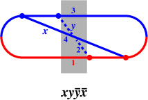
Figure 11: The canonical “crossed” diagram. Particles in the (shaded) region of 4-particle evolution are numbered according to the convention of ref. 2brem .

5.1 Allowed Color Transitions

At the start of the shaded region of 4-particle evolution, the particles combine in the same way as for the sequential diagram of fig. 8, and so the initial 4-particle color singlet state is the same as before:

$$|{\rm A}_{\rm aa}\rangle_{u}=\tfrac{1}{\sqrt{2}}|{\rm A}_{+}\rangle+\tfrac{1}{\sqrt{2}}|{\rm A}_{-}\rangle\qquad\mbox{(initial 4-particle state)}.$$ (78)

However, the end of the shaded region is different: It is now gluons 1 and 2 that meet at a vertex. So, the final state is the $s$-channel version $|{\rm A}_{\rm aa}\rangle_{s}$ rather than $u$-channel version (78). In this paper, we find it convenient to always stick to the definition (13) of our basis states $(1,{\rm A}_{+},{\rm A}_{-},{\rm A}^{\!\times},1^{\times}_{+},1^{\times}_{-})$, which are defined in terms of $u$-channel singlet combinations. We need to figure out how to express our final ($s$-channel) color singlet state $|{\rm A}_{\rm aa}\rangle_{s}$ in terms of this basis. The matrix that converts (for any $N$) between the $s$-channel and $u$-channel versions of the original basis states (7) is given by color ; NSZ6j ; Sjodahl (see appendix A.1)

$$\begin{pmatrix}|{\bm{1}}\rangle_{s}\\ |{\rm A}_{\rm aa}\rangle_{s}\\ |{\rm A}_{\rm ss}\rangle_{s}\\ |``\bm{10}{+}\overline{\bm{10}}"\rangle_{s}\\ |``\bm{27}"\rangle_{s}\\ |``\bm{0}"\rangle_{s}\end{pmatrix}=\mathds{U}\begin{pmatrix}|{\bm{1}}\rangle_{u}\\ |{\rm A}_{\rm aa}\rangle_{u}\\ |{\rm A}_{\rm ss}\rangle_{u}\\ |``\bm{10}{+}\overline{\bm{10}}"\rangle_{u}\\ |``\bm{27}"\rangle_{u}\\ |``\bm{0}"\rangle_{u}\end{pmatrix}$$ (79a)

with

$$\mathds{U}=\begin{pmatrix}\tfrac{1}{N^{2}-1}&-\sqrt{\tfrac{1}{N^{2}-1}}&\sqrt{\tfrac{1}{N^{2}-1}}&-\sqrt{\tfrac{N^{2}-4}{2(N^{2}-1)}}&\tfrac{N}{2(N+1)}\sqrt{\tfrac{N+3}{N-1}}&\tfrac{N}{2(N-1)}\sqrt{\tfrac{N-3}{N+1}}\\[5.0pt] &\tfrac{1}{2}&-\tfrac{1}{2}&0&\tfrac{1}{2}\sqrt{\tfrac{N+3}{N+1}}&-\tfrac{1}{2}\sqrt{\tfrac{N-3}{N-1}}\\ &&\tfrac{N^{2}-12}{2(N^{2}-4)}&\sqrt{\tfrac{2}{N^{2}-4}}&\tfrac{N}{2(N+2)}\sqrt{\tfrac{N+3}{N+1}}&-\tfrac{N}{2(N-2)}\sqrt{\tfrac{N-3}{N-1}}\\[5.0pt] &&&\tfrac{1}{2}&\sqrt{\tfrac{(N-2)(N+3)}{8(N+1)(N+2)}}&\sqrt{\tfrac{(N+2)(N-3)}{8(N-1)(N-2)}}\\[5.0pt] \lx@intercol\hfil\rm(symmetric)\hfil\lx@intercol&&\tfrac{N^{2}+N+2}{4(N+1)(N+2)}&\tfrac{1}{4}\sqrt{\tfrac{N^{2}-9}{N^{2}-1}}\\[5.0pt] &&&&&\tfrac{N^{2}-N+2}{4(N-1)(N-2)}\\ \end{pmatrix}.$$ (79b)

For our present purpose, the only piece of (79) that we need is

$$|{\rm A}_{\rm aa}\rangle_{s}=-\sqrt{\tfrac{1}{N^{2}-1}}\,|{\bm{1}}\rangle_{u}+\tfrac{1}{2}\,|{\rm A}_{\rm aa}\rangle_{u}-\tfrac{1}{2}\,|{\rm A}_{\rm ss}\rangle_{u}+\tfrac{1}{2}\sqrt{\tfrac{N+3}{N+1}}\,|``\bm{27}"\rangle_{u}-\tfrac{1}{2}\sqrt{\tfrac{N-3}{N-1}}\,|``\bm{0}"\rangle_{u}.$$ (80)

Using (13) to convert to the basis states $(1,{\rm A}_{+},{\rm A}_{-},{\rm A}^{\!\times},1^{\times}_{+},1^{\times}_{-})$ that we use for our analysis in this paper, and then expanding in $1/N$,

$$|{\rm A}_{\rm aa}\rangle_{s}=\frac{|{\rm A}_{-}\rangle+|{\rm A}^{\!\times}\rangle}{\sqrt{2}}+\frac{|1^{\times}_{+}\rangle+|1^{\times}_{-}\rangle-2|1\rangle}{2N}-\frac{3|{\rm A}^{\!\times}\rangle}{2\sqrt{2}\,N^{2}}+O(N^{-3})\\ \mbox{(final 4-particle state)}.$$ (81)

For future reference, note that the overall sign of $|{\rm A}_{\rm aa}\rangle_{s}$ is merely a phase convention choice for that state. Different choices of this sign convention must lead to compensating changes of sign in the rule for the diagrammatic vertex at the end of the 4-particle evolution in fig. 11. We will later discuss how to get the overall sign of our answer right without having to drill down into such details.

We may now using the initial and final singlet states (78) and (81), together with the textures of the perturbations $\delta\underline{S}$, $\delta\underline{T}$ and $\delta^{2}\underline{T}$ of (17), to list all possible 4-particle color transition sequences that contribute to $1/N^{2}$ corrections to the $xy\bar{y}\bar{x}$ diagram of fig. 11. They are listed in table 1.

transition	equivalent	$\delta S$, $\delta T$, $\delta^{2}T$ factors	color . overlap	$\phi$
$|{\rm A}_{-}\rangle\xrightarrow{\delta T}{}\kern 3.09998pt|1\rangle\kern 3.09998pt\xrightarrow{\delta T}|{\rm A}_{-}\rangle$	$(1234)\to(41)(23)\to(1234)$	$\tfrac{1}{2N^{2}}$	$\tfrac{1}{2}$	$\frac{1}{2N^{2}}$
$|{\rm A}_{-}\rangle\xrightarrow{\delta T}{}|1^{\times}_{-}\rangle\xrightarrow{\delta T}|{\rm A}_{-}\rangle$	$(1234)\to(12)(34)\to(1234)$	$\tfrac{1}{2N^{2}}$	$\tfrac{1}{2}$	$\frac{1}{2N^{2}}$
$|{\rm A}_{+}\rangle\xrightarrow{\delta T}{}\kern 3.09998pt|1\rangle\kern 3.09998pt\xrightarrow{\delta T}|{\rm A}_{-}\rangle$	$(1324)\to(41)(23)\to(1234)$	$\tfrac{1}{2N^{2}}$	$\tfrac{1}{2}$	$\frac{1}{2N^{2}}$
$|{\rm A}_{-}\rangle\xrightarrow{\delta T}{}|1^{\times}_{-}\rangle\xrightarrow{\delta S}|{\rm A}^{\!\times}\rangle$	$(1234)\to(12)(34)\to(1243)$	$-\tfrac{1}{2N^{2}}$	$\tfrac{1}{2}$	$-\frac{1}{2N^{2}}$
$|{\rm A}_{+}\rangle\xrightarrow{\delta T}{}|1^{\times}_{+}\rangle\xrightarrow{\delta S}|{\rm A}^{\!\times}\rangle$	$(1324)\to(13)(24)\to(1243)$	$-\tfrac{1}{2N^{2}}$	$\tfrac{1}{2}$	$-\frac{1}{2N^{2}}$
$|{\rm A}_{-}\rangle\xrightarrow{\delta^{2}T}{}|{\rm A}^{\!\times}\rangle$	$(1234)\to(1243)$	$\tfrac{1}{2N^{2}}$	$\tfrac{1}{2}$	$\frac{1}{2N^{2}}$
$|{\rm A}_{+}\rangle\xrightarrow{\delta^{2}T}{}|{\rm A}^{\!\times}\rangle$	$(1324)\to(1243)$	$\tfrac{1}{2N^{2}}$	$\tfrac{1}{2}$	$\frac{1}{2N^{2}}$
$|{\rm A}_{-}\rangle\xrightarrow{\delta T}{}\kern 3.09998pt|1\rangle\kern 3.09998pt$	$(1234)\to(41)(23)$	$\tfrac{1}{\sqrt{2}\,N}$	$-\tfrac{1}{\sqrt{2}\,N}$	$-\frac{1}{N^{2}}$
$|{\rm A}_{-}\rangle\xrightarrow{\delta T}{}|1^{\times}_{-}\rangle$	$(1234)\to(12)(34)$	$\tfrac{1}{\sqrt{2}\,N}$	$\tfrac{1}{2\sqrt{2}\,N}$	$\frac{1}{2N^{2}}$
$|{\rm A}_{+}\rangle\xrightarrow{\delta T}{}\kern 3.09998pt|1\rangle\kern 3.09998pt$	$(1324)\to(41)(23)$	$\tfrac{1}{\sqrt{2}\,N}$	$-\tfrac{1}{\sqrt{2}\,N}$	$-\frac{1}{N^{2}}$
$|{\rm A}_{+}\rangle\xrightarrow{\delta T}{}|1^{\times}_{+}\rangle$	$(1324)\to(13)(24)$	$\tfrac{1}{\sqrt{2}\,N}$	$\tfrac{1}{2\sqrt{2}\,N}$	$\frac{1}{2N^{2}}$

Table 1: Allowed 4-particle color transitions at order $1/N^{2}$ for the $xy\bar{y}\bar{x}$ diagram, along with (i) the associated $\delta T$, $\delta S$ or $\delta^{2}T$ factors, and (ii) the product of the initial and final color overlap factors $\langle\lambda_{\rm i}|{\rm A}_{\rm aa}\rangle_{u}$ and ${}_{s}\langle{\rm A}_{\rm aa}|\lambda_{\rm f}\rangle$. Also shown is the product $\phi$ of (i) and (ii) relative to what it would be $\bigl{[}\,{}_{s}\langle{\rm A}_{\rm aa}|{\rm A}_{-}\rangle\langle{\rm A}_{-}|{\rm A}_{\rm aa}\rangle_{u}\,{=}\,\tfrac{1}{2}\,\bigr{]}$ in the $N{=}\infty$ calculation of the crossed diagram. The horizontal lines separate groups of processes that have to be handled differently: 2nd order in $\delta V$ with two $\delta T$ transitions; 2nd order in $\delta V$ with a $\delta T$ and $\delta S$ transition; 1st order in $\delta V$ with a $T$-based perturbation. There are no non-zero $O(1/N^{2})$ contributions at 0th order in $\delta\underline{V}$. [Specifically, the $1/N^{2}$ term in (81) for the final state $|A_{\rm aa}\rangle_{s}$ does not directly overlap the initial state $|A_{\rm aa}\rangle_{u}$ of (23).]

5.2 2nd order in $\delta V$

We start by examining the first five lines of table 1, which are the cases that involve two insertions of perturbations $\delta\underline{V}$ in the 4-particle evolution. Schematically, these cases correspond to fig. 12, which is the crossed diagram analog of fig. 9. The formulas for these contributions to the crossed diagram $xy\bar{y}\bar{x}$ are basically the same as the formulas we found in section 3 for the sequential diagram $xy\bar{x}\bar{y}$ except for some minor modifications. One modification is simply that we should use the color transitions given by the first five lines of table 1 instead of the sequential diagram transitions of (24). But there are other changes needed as well.

Figure 12: The analog of fig. 9, now for the $xy\bar{y}\bar{x}$ crossed diagram.

5.2.1 Modification: $(X,Y,Z)$

The known $N{=}\infty$ rate for the $xy\bar{y}\bar{x}$ diagram has a form similar to that quoted earlier for the ${\rm A}_{-}{=}(1234)$ color routing of the $xy\bar{x}\bar{y}$ diagram in (47). The $xy\bar{y}\bar{x}$ case is 2brem

$$\left[\frac{d\Gamma}{dx\,dy}\right]_{xy\bar{y}\bar{x}}=-\int_{0}^{\infty} d(\Delta t)\>\frac{C_{\rm A}^{2}\alpha_{\rm s}^{2}M_{\rm i}M_{\rm f}}{8\pi^{2}(x_{1}{+}x_{4})^{2}E^{4}}\,f_{{\rm A}_{-}}$$

$$\times\Bigl{\{}(\beta Y_{\rm y}Y_{\bar{\rm y}}+\alpha\overline{Y}_{{\rm y}{\bar{\rm y}}}Y_{{\rm y}{\bar{\rm y}}})I_{0}+(\alpha+\beta+2\gamma)Z_{{\rm y}{\bar{\rm y}}}I_{1}$$

$$\quad+\bigl{[}(\alpha+\gamma)Y_{\rm y}Y_{\bar{\rm y}}+(\beta+\gamma)\overline{Y}_{{\rm y}{\bar{\rm y}}}Y_{{\rm y}{\bar{\rm y}}}\bigr{]}I_{2}$$

$$\quad-(\alpha+\beta+\gamma)(\overline{Y}_{{\rm y}{\bar{\rm y}}}Y_{\bar{\rm y}}I_{3}+Y_{\rm y}Y_{{\rm y}{\bar{\rm y}}}I_{4})\Bigl{\}}.$$ (82)

The $(\alpha,\beta,\gamma)$ are different combinations of helicity-dependent DGLAP splitting functions than those in the sequential case, and their formulas may be found in ref. 2brem . The $I_{n}$ here have the same form as the $I_{n}^{\rm seq}$ of (48) except that the superscript “${\rm seq}$” should be removed from everything. However, the $(X,Y,Z)$’s are somewhat different from the $(X^{\rm seq},Y^{\rm seq},Z^{\rm seq})$’s. In the original $N{=}\infty$ calculation 2brem , they were defined so that the exponential factor in the 4-particle propagator was

$$\exp\Biggl{[}-\frac{1}{2}\begin{pmatrix}{\bm{C}}_{41}^{\rm y}\\ {\bm{C}}_{23}^{\rm y}\end{pmatrix}^{\!\!\top}\!\begin{pmatrix}{\cal X}_{\rm y}&Y_{\rm y}\\ Y_{\rm y}&Z_{\rm y}\end{pmatrix}\begin{pmatrix}{\bm{C}}_{41}^{\rm y}\\ {\bm{C}}_{23}^{\rm y}\end{pmatrix}-\frac{1}{2}\begin{pmatrix}{\bm{C}}_{34}^{\bar{\rm y}}\\ {\bm{C}}_{12}^{\bar{\rm y}}\end{pmatrix}^{\!\!\top}\!\begin{pmatrix}{\cal X}_{\bar{\rm y}}&Y_{\bar{\rm y}}\\ Y_{\bar{\rm y}}&Z_{\bar{\rm y}}\end{pmatrix}\begin{pmatrix}{\bm{C}}_{34}^{\bar{\rm y}}\\ {\bm{C}}_{12}^{\bar{\rm y}}\end{pmatrix}\\ +\begin{pmatrix}{\bm{C}}_{41}^{\rm y}\\ {\bm{C}}_{23}^{\rm y}\end{pmatrix}^{\!\!\top}\!\begin{pmatrix}X_{{\rm y}{\bar{\rm y}}}&Y_{{\rm y}{\bar{\rm y}}}\\ \overline{Y}_{{\rm y}{\bar{\rm y}}}&Z_{{\rm y}{\bar{\rm y}}}\end{pmatrix}\begin{pmatrix}{\bm{C}}_{34}^{\bar{\rm y}}\\ {\bm{C}}_{12}^{\bar{\rm y}}\end{pmatrix}\Biggr{]},$$ (83)

where

$$X_{\rm y} =|M_{\rm i}|\Omega_{\rm i}+{\cal X}_{\rm y},$$ (84a)

$$X_{\bar{\rm y}} =|M_{\rm f}|\Omega_{\rm f}+{\cal X}_{\bar{\rm y}}$$ (84b)

similar to (50). Explicit formulas for $M_{\rm i}$, $\Omega_{\rm i}$, $M_{\rm f}$, $\Omega_{\rm f}$ may be found in ref. 2brem .

The pattern common to the presentations (42) and (83) of the sequential and crossed exponentials is that in each vector, the bottom ${\bm{C}}_{ij}^{v}$ is the one for which lines $i$ and $j$ come together at the corresponding vertex $v$ of the diagram. It was the use of this convention that made the $N{=}\infty$ rate formulas (47) and (82) for sequential and crossed diagrams have similar structure.

Similar to what happened for the sequential diagram, (83) for this crossed diagram just gives particular names to the entries of the matrices that in this paper we would call $A_{{\rm A}_{-}}$ and $B_{{\rm A}_{-}}$ — the identically same matrices that were relevant to the case of sequential diagrams in (43). Here the relations are

$$A_{{\rm A}_{-}}=\begin{pmatrix}{\cal X}_{\rm y}&Y_{\rm y}\\ Y_{\rm y}&Z_{\rm y}\end{pmatrix}={\mathfrak{S}}^{-1\top}\begin{pmatrix}{\cal X}_{\bar{\rm y}}&Y_{\bar{\rm y}}\\ Y_{\bar{\rm y}}&Z_{\bar{\rm y}}\end{pmatrix}{\mathfrak{S}}^{-1},\qquad B_{{\rm A}_{-}}=\begin{pmatrix}X_{{\rm y}{\bar{\rm y}}}&Y_{{\rm y}{\bar{\rm y}}}\\ \overline{Y}_{{\rm y}{\bar{\rm y}}}&\tilde{Z}_{{\rm y}{\bar{\rm y}}}\end{pmatrix}{\mathfrak{S}}^{-1},$$ (85a)

where ${\mathfrak{S}}$ is the matrix from (66) that converts the $(C_{34},C_{12})$ basis into the $(C_{41},C_{23})$ basis:

$$\begin{pmatrix}{\bm{C}}_{41}\\ {\bm{C}}_{23}\end{pmatrix}={\mathfrak{S}}\begin{pmatrix}{\bm{C}}_{34}\\ {\bm{C}}_{12}\end{pmatrix}$$ (86a)

with

$${\mathfrak{S}}\equiv\frac{1}{(x_{1}{+}x_{4})}\begin{pmatrix}-x_{3}&-x_{2}\\ \phantom{-}x_{4}&\phantom{-}x_{1}\end{pmatrix}.$$ (86b)

Like we did for the sequential $xy\bar{x}\bar{y}$ diagram, we now want to put the exponential factor

$$e^{-\frac{1}{2}\vec{\bm{z}}^{\top}({\cal A}-{\cal B}\,{\cal U}^{-1}{\cal B})\vec{\bm{z}}}$$ (87)

for the $1/N^{2}$ correction into the same form as the exponential factor (83) for the known $N{=}\infty$ result. Since (87) is exactly the same as before, the only difference is in the identification of the $(X,Y,Z)$’s. By comparing (85) with the sequential version (43), we can read off the relation of the $(X,Y,Z)$’s of the crossed diagram with the previously identified $(X,Y,Z)^{\rm seq}$ of the sequential diagram:

$$\begin{pmatrix}\tilde{\cal X}_{\rm y}&\tilde{Y}_{\rm y}\\[2.0pt] \tilde{Y}_{\rm y}&\tilde{Z}_{\rm y}\end{pmatrix}=\begin{pmatrix}\tilde{\cal X}_{\rm y}^{\rm seq}&\tilde{Y}_{\rm y}^{\rm seq}\\[2.0pt] \tilde{Y}_{\rm y}^{\rm seq}&\tilde{Z}_{\rm y}^{\rm seq}\end{pmatrix},\qquad\begin{pmatrix}\tilde{\cal X}_{\bar{\rm y}}&\tilde{Y}_{\bar{\rm y}}\\[2.0pt] \tilde{Y}_{\bar{\rm y}}&\tilde{Z}_{\bar{\rm y}}\end{pmatrix}={\mathfrak{S}}^{\top}{\cal S}\begin{pmatrix}\tilde{\cal X}_{\bar{\rm x}}^{\rm seq}&\tilde{Y}_{\bar{\rm x}}^{\rm seq}\\[2.0pt] \tilde{Y}_{\bar{\rm x}}^{\rm seq}&\tilde{Z}_{\bar{\rm x}}^{\rm seq}\end{pmatrix}{\cal S}{\mathfrak{S}},$$ (88a)

$$\begin{pmatrix}\tilde{X}_{{\rm y}{\bar{\rm y}}}&\tilde{Y}_{{\rm y}{\bar{\rm y}}}\\[2.0pt] \tilde{\overline{Y}}_{{\rm y}{\bar{\rm y}}}&\tilde{Z}_{{\rm y}{\bar{\rm y}}}\end{pmatrix}=\begin{pmatrix}\tilde{X}_{{\rm y}{\bar{\rm x}}}^{\rm seq}&\tilde{Y}_{{\rm y}{\bar{\rm x}}}^{\rm seq}\\[2.0pt] \tilde{\overline{Y}}_{{\rm y}{\bar{\rm x}}}^{\rm seq}&\tilde{Z}_{{\rm y}{\bar{\rm x}}}^{\rm seq}\end{pmatrix}{\cal S}{\mathfrak{S}},$$ (88b)

where ${\cal S}$ is again defined by (44). So, to compute $(\tilde{X},\tilde{Y},\tilde{Z})$’s for the crossed diagrams, first compute ${\cal A}-{\cal B}\,{\cal U}^{-1}{\cal B}$ as in section 3, then read out the $(\tilde{X},\tilde{Y},\tilde{Z})^{\rm seq}$ values using (46), and finally convert those values using (88) above.

5.2.2 Modification: the matrix $R_{2}$

The identification of the $2{\times}2$ matrices $R_{1}=R_{2}=R^{(\delta T)}$ back in (29) was based on the fact that only $\delta T$ transitions (24) were relevant for the sequential diagram $xy\bar{x}\bar{y}$. The same is true for the first three rows of table 1, which shows the allowed transition sequences for the crossed diagram $xy\bar{y}\bar{x}$. We will refer to those first three rows as “$\delta T\,\delta T$” transition sequences.

In the next two rows of the table, however, the second transition of each sequence is instead a $\delta S$ transition. We will refer to these rows as “$\delta T\,\delta S$” transition sequences. $\underline{S}_{u}$ appears differently than $\underline{T}_{u}$ in the potential (8b), and so its contribution to $\delta\underline{V}$ matrix elements will be different than those of the $\delta T$ contribution (28). The non-zero matrix elements associated with $\delta\underline{S}$ are

$$\delta V^{(\delta S)}\!(\vec{\bm{\xi}})=\frac{i\hat{q}_{\rm A}}{2\sqrt{2}\,N}\Bigl{[}x_{4}x_{1}C_{41}^{2}+x_{2}x_{3}C_{23}^{2}+\tfrac{1}{2}(x_{4}-x_{1})(x_{2}-x_{3}){\bm{C}}_{41}\cdot{\bm{C}}_{23}\Bigr{]},$$ (89)

which can be written in the form of $\tfrac{1}{2}\vec{\bm{\xi}}^{\,\top}R^{(\delta S)}\vec{\bm{\xi}}$ with

$$R^{(\delta S)}=+\frac{i\hat{q}_{\rm A}}{2\sqrt{2}\,N}\begin{pmatrix}2x_{1}x_{4}&\tfrac{1}{2}(x_{4}{-}x_{1})(x_{2}{-}x_{3})\\ \tfrac{1}{2}(x_{4}{-}x_{1})(x_{2}{-}x_{3})&2x_{2}x_{3}\end{pmatrix}.$$ (90)

So, the final rule is that we need to use

$$(R_{1},R_{2})=\begin{cases}(R^{(\delta T)},R^{(\delta T)})&\mbox{for $\delta T\,\delta T$ transitions};\\ (R^{(\delta T)},R^{(\delta S)})&\mbox{for $\delta T\,\delta S$ transitions}\end{cases}$$ (91)

in the construction (39a) of the $4{\times}4$ matrix ${\cal U}$.

5.2.3 Final result for 2nd order in $\delta V$

With the preceding modifications, the final result for the first five rows of table 1 has the same relation to (82) that the sequential result (51) did to (47):

$$\delta^{2}\left[\frac{d\Gamma}{dx\,dy}\right]_{xy\bar{y}\bar{x}}^{(\delta V)^{2}} ={}\frac{C_{\rm A}^{2}\alpha_{\rm s}^{2}M_{\rm i}M_{\rm f}}{8\pi^{2}(x_{1}{+}x_{4})^{2}E^{4}}\sum_{\begin{subarray}{c}{\rm allowed}\\ \lambda_{01},\lambda_{12},\lambda_{23}\end{subarray}}\int_{0<t_{1}<t_{2}<\Delta t}dt_{1}\>dt_{2}\>d(\Delta t)\>(2\pi)^{4}f_{(01)}f_{(12)}f_{(23)}$$

$$\quad\times\frac{d}{dj_{1}}\,\frac{d}{dj_{2}}\biggl{[}\det({\cal U}^{-1})\Bigl{\{}(\beta\tilde{Y}_{\rm y}\tilde{Y}_{\bar{\rm y}}+\alpha\tilde{\overline{Y}}_{{\rm y}{\bar{\rm y}}}\tilde{Y}_{{\rm y}{\bar{\rm y}}})\tilde{I}_{0}+(\alpha+\beta+2\gamma)\tilde{Z}_{{\rm y}{\bar{\rm y}}}\tilde{I}_{1}$$

$$\hskip 60.00009pt+\bigl{[}(\alpha+\gamma)\tilde{Y}_{\rm y}\tilde{Y}_{\bar{\rm y}}+(\beta+\gamma)\tilde{\overline{Y}}_{{\rm y}{\bar{\rm y}}}\tilde{Y}_{{\rm y}{\bar{\rm y}}}\bigr{]}\tilde{I}_{2}$$

$$\hskip 60.00009pt-(\alpha+\beta+\gamma)(\tilde{\overline{Y}}_{{\rm y}{\bar{\rm y}}}\tilde{Y}_{\bar{\rm y}}\tilde{I}_{3}+\tilde{Y}_{\rm y}\tilde{Y}_{{\rm y}{\bar{\rm y}}}\tilde{I}_{4})\Bigl{\}}\biggr{]}_{j_{1}=j_{2}=0}.$$ (92)

In the context of the sequential $xy\bar{x}\bar{y}$ diagram, we previously discussed that equality of initial and final 4-particle color singlet state overlap factors between (i) the calculation of $1/N^{2}$ corrections in (52) and (ii) the $N{=}\infty$ calculation in (53). A similar match-up occurs for the first five rows of table 1. Specifically, the calculation of those $1/N^{2}$ corrections should contain a factor of

$${}_{s}\langle{\rm A}_{\rm aa}|\lambda_{23}\rangle\langle\lambda_{01}|{\rm A}_{\rm aa}\rangle_{u}=\tfrac{1}{2}.$$ (93)

But we did not have to explicitly include that factor because our starting point — the $N{=}\infty$ formula (82) for the crossed diagram $xy\bar{x}\bar{y}$ — already implicitly contained an equal factor of

$${}_{s}\langle{\rm A}_{\rm aa}|{\rm A}_{-}\rangle\langle{\rm A}_{-}|{\rm A}_{\rm aa}\rangle_{u}=\tfrac{1}{2}.$$ (94)

5.3 A single $\delta T$ or $\delta^{2}T$ perturbation

We now turn to the last group of transitions in table 1, where there is only one $\delta T$ or $\delta^{2}T$ perturbation. Schematically, this corresponds to fig. 13. The analog of (26) is

$$\delta G_{\lambda_{12}\leftarrow\lambda_{01}}(\vec{\bm{\xi}}_{2},\Delta t;\vec{\bm{\xi}}_{0},0)$$

$$\qquad=-i\int_{0<t_{1}<\Delta t}dt_{1}\>\int_{\vec{\bm{\xi}}_{1}}G^{N=\infty}_{\lambda_{12}}(\vec{\bm{\xi}}_{2},t_{2};\vec{\bm{\xi}}_{1},t_{1})\,\delta V_{\lambda_{12}\leftarrow\lambda_{01}}^{(\delta^{n}T)}\!(\vec{\bm{\xi}}_{1})\,G^{N=\infty}_{\lambda_{01}}(\vec{\bm{\xi}}_{1},t_{1};\vec{\bm{\xi}}_{0},t_{0}),$$ (95)

where $t_{0}=t^{\rm y}$ and $t_{2}=t^{\bar{\rm y}}$ are the initial and final times of the 4-particle evolution. The analog of (38) is then

$$\delta G_{\lambda_{12}\leftarrow\lambda_{01}}(\vec{\bm{\xi}}_{2},\Delta t;\vec{\bm{\xi}}_{0},0)=-if_{(01)}f_{(12)}\int_{0<t_{1}<\Delta t}dt_{1}\>e^{-\frac{1}{2}\vec{\bm{\xi}}_{0}^{\,\top}\!A_{(01)}\,\vec{\bm{\xi}}_{0}-\frac{1}{2}\vec{\bm{\xi}}_{2}^{\,\top}\!A_{(12)}\,\vec{\bm{\xi}}_{2}}\\ \times\frac{d}{dj_{1}}\int d^{2}\xi_{1}\>e^{-\frac{1}{2}\vec{\bm{\xi}}_{1}^{\top}\!U\vec{\bm{\xi}}_{1}}e^{\,\vec{\bm{\xi}}_{1}^{\,\top}\left(B_{(01)}\vec{\bm{\xi}}_{0}+B_{(12)}\vec{\bm{\xi}}_{2}\right)}\>\biggr{|}_{j_{1}=0},$$ (96)

where

$$U\equiv A_{(01)}+A_{(12)}-j_{1}R_{1}.$$ (97)

Doing the Gaussian integral over $\vec{\bm{\xi}}_{1}$ yields the analog of (41):

$$\delta G_{\lambda_{12}\leftarrow\lambda_{01}}(\vec{\bm{\xi}}_{2},\Delta t;\vec{\bm{\xi}}_{0},0)=$$

$$\qquad-i(2\pi)^{2}f_{(01)}f_{(12)}\int_{0<t_{1}<\Delta t}dt_{1}\>\frac{d}{dj_{1}}\biggl{[}\det(U^{-1})\,e^{-\frac{1}{2}\vec{\bm{\xi}}_{0}^{\,\top}\!A_{(01)}\,\vec{\bm{\xi}}_{0}-\frac{1}{2}\vec{\bm{\xi}}_{2}^{\,\top}\!A_{(12)}\,\vec{\bm{\xi}}_{2}+\frac{1}{2}\vec{\bm{J}}^{\,\top}\!U^{-1}\vec{\bm{J}}}\biggr{]}_{j_{1}=0}$$ (98a)

with

$$\vec{\bm{J}}\equiv B_{(01)}\vec{\bm{\xi}}_{0}+B_{(12)}\vec{\bm{\xi}}_{2}\,.$$ (98b)

Figure 13: Like fig. 12 except with only one insertion of $\delta V$ (or $\delta^{2}V$) during the 4-particle time evolution.

By comparison of the exponential in (98) to the $N{=}\infty$ exponential in (83), and accounting for the change of basis (86), we find that for these processes

$$\begin{pmatrix}\tilde{\cal X}_{\rm y}&\tilde{Y}_{\rm y}\\ \tilde{Y}_{\rm y}&\tilde{Z}_{\rm y}\end{pmatrix}=A_{(01)}-B_{(01)}U^{-1}B_{(01)},\qquad\begin{pmatrix}\tilde{\cal X}_{\bar{\rm y}}&\tilde{Y}_{\bar{\rm y}}\\ \tilde{Y}_{\bar{\rm y}}&\tilde{Z}_{\bar{\rm y}}\end{pmatrix}={\mathfrak{S}}^{\top}(A_{(12)}-B_{(12)}U^{-1}B_{(12)}){\mathfrak{S}},$$ (99a)

$$\begin{pmatrix}\tilde{X}_{{\rm y}{\bar{\rm y}}}&\tilde{Y}_{{\rm y}{\bar{\rm y}}}\\ \tilde{\overline{Y}}_{{\rm y}{\bar{\rm y}}}&\tilde{Z}_{{\rm y}{\bar{\rm y}}}\end{pmatrix}=B_{(01)}U^{-1}B_{(12)}{\mathfrak{S}}.$$ (99b)

Also, as before, the $\cal X$’s are related to the $X$’s by (84). The analog of (92) is then

$$\delta^{2}\left[\frac{d\Gamma}{dx\,dy}\right]_{xy\bar{y}\bar{x}}^{\delta T\,{\rm or}\,\delta^{2}T}={} i\frac{C_{\rm A}^{2}\alpha_{\rm s}^{2}M_{\rm i}M_{\rm f}}{8\pi^{2}(x_{1}{+}x_{4})^{2}E^{4}}\sum_{\begin{subarray}{c}{\rm allowed}\\ \lambda_{01},\lambda_{12}\end{subarray}}\Phi_{\lambda_{01},\lambda_{12}}\int_{0<t_{1}<\Delta t}\!\!\!\!dt_{1}\>d(\Delta t)\>(2\pi)^{2}f_{(01)}f_{(12)}$$

$$\quad\times\frac{d}{dj_{1}}\biggl{[}\det(U^{-1})\Bigl{\{}(\beta\tilde{Y}_{\rm y}\tilde{Y}_{\bar{\rm y}}+\alpha\tilde{\overline{Y}}_{{\rm y}{\bar{\rm y}}}\tilde{Y}_{{\rm y}{\bar{\rm y}}})\tilde{I}_{0}+(\alpha+\beta+2\gamma)\tilde{Z}_{{\rm y}{\bar{\rm y}}}\tilde{I}_{1}$$

$$\hskip 60.00009pt+\bigl{[}(\alpha+\gamma)\tilde{Y}_{\rm y}\tilde{Y}_{\bar{\rm y}}+(\beta+\gamma)\tilde{\overline{Y}}_{{\rm y}{\bar{\rm y}}}\tilde{Y}_{{\rm y}{\bar{\rm y}}}\bigr{]}\tilde{I}_{2}$$

$$\hskip 60.00009pt-(\alpha+\beta+\gamma)(\tilde{\overline{Y}}_{{\rm y}{\bar{\rm y}}}\tilde{Y}_{\bar{\rm y}}\tilde{I}_{3}+\tilde{Y}_{\rm y}\tilde{Y}_{{\rm y}{\bar{\rm y}}}\tilde{I}_{4})\Bigl{\}}\biggr{]}_{j_{1}=0},$$ (100)

where the $(\tilde{X},\tilde{Y},\tilde{Z})$’s are now those determined by (99) and the $\Phi_{\lambda_{01},\lambda_{12}}$ is a normalization factor we discuss below.

For simplicity, we will take

$$R_{1}=R^{(\delta T)}$$ (101)

in the definition (97) of $U$ for all of the single $\delta V$ processes summarized in table 2. Because we are using (101) for $\delta^{2}T$ as well as $\delta T$ perturbations, this leads to the first of two normalization issues.

transition	equivalent	$\Phi$
$|{\rm A}_{-}\rangle\xrightarrow{\delta^{2}T}{}|{\rm A}^{\!\times}\rangle$	$(1234)\to(1243)$	$\frac{1}{\sqrt{2}\,N}$
$|{\rm A}_{+}\rangle\xrightarrow{\delta^{2}T}{}|{\rm A}^{\!\times}\rangle$	$(1324)\to(1243)$	$\frac{1}{\sqrt{2}\,N}$
$|{\rm A}_{-}\rangle\xrightarrow{\delta T}{}\kern 3.09998pt|1\rangle\kern 3.09998pt$	$(1234)\to(14)(23)$	$\frac{-2}{\sqrt{2}\,N}$
$|{\rm A}_{-}\rangle\xrightarrow{\delta T}{}|1^{\times}_{-}\rangle$	$(1234)\to(12)(34)$	$\frac{1}{\sqrt{2}\,N}$
$|{\rm A}_{+}\rangle\xrightarrow{\delta T}{}\kern 3.09998pt|1\rangle\kern 3.09998pt$	$(1324)\to(14)(23)$	$\frac{-2}{\sqrt{2}\,N}$
$|{\rm A}_{+}\rangle\xrightarrow{\delta T}{}|1^{\times}_{+}\rangle$	$(1324)\to(13)(24)$	$\frac{1}{\sqrt{2}\,N}$

Table 2: The last group of transition sequences from table 1, along with the corresponding factor $\Phi$ appearing in (100).

The operation ${\partial/\partial j_{1}}[\cdots]_{j_{1}=0}$ in (100) was constructed to introduce one factor of $\tfrac{1}{2}\vec{\bm{\xi}}_{1}^{\,\top}R_{1}\vec{\bm{\xi}}_{1}$ (unexponentiated) into the calculation of the overall result. Based on (17), $\delta^{2}T$ matrix elements relevant to the transitions in table 2 all have value $1/2N^{2}$. In contrast, the non-zero matrix elements of $\delta T$ in (17) are all $1/\sqrt{2}\,N$. To correct for this difference, our overall factor $\Phi$ in (100) will need to contain (among other things) a factor of

$$\begin{cases}1,&\mbox{for $\,\delta T\,$ transition};\\ \frac{1}{\sqrt{2}\,N},&\mbox{for $\delta^{2}T$ transition}.\end{cases}$$ (102)

Earlier, we explained that our starting point — the $N{=}\infty$ result — implicitly contains an initial and final color singlet overlap factor (94), which equals the similar overlap factors ${}_{s}\langle{\rm A}_{\rm aa}|\lambda_{23}\rangle\langle\lambda_{01}|{\rm A}_{\rm aa}\rangle_{u}$ needed for both $\delta T\,\delta T$ and $\delta T\,\delta S$ transition sequences. From the “color overlap” column of table 1, however, we see that these overlap factors are different for some of the other transition sequences. Our overall normalization in (100) will need to account for this difference as well. Putting that correction together with (102), the overall normalization correction we need in (100) is

$$\Phi_{\lambda_{01},\lambda_{12}} \equiv\frac{{}_{s}\langle{\rm A}_{\rm aa}|\lambda_{12}\rangle\langle\lambda_{01}|{\rm A}_{\rm aa}\rangle_{u}}{{}_{s}\langle{\rm A}_{\rm aa}|{\rm A}_{-}\rangle\langle{\rm A}_{-}|{\rm A}_{\rm aa}\rangle_{u}}\times\frac{\mbox{$\delta T$ or $\delta^{2}T$ matrix element}}{\mbox{non-zero $\delta T$ matrix elements}}$$

$$=2\,{}_{s}\langle{\rm A}_{\rm aa}|\lambda_{12}\rangle\langle\lambda_{01}|{\rm A}_{\rm aa}\rangle_{u}\times\begin{cases}1,&\mbox{for $\,\delta T\,$ transition};\\ \frac{1}{\sqrt{2}\,N},&\mbox{for $\delta^{2}T$ transition}.\end{cases}$$ (103)

The values of $\Phi$ are shown explicitly in Table 2. (They are the same as $\sqrt{2}\,N\phi$, where $\phi$ is the last column of table 1.)

Note that the $1/N^{2}$ behavior of (100) comes from two places: One factor of $1/N$ comes from the factor $R_{1}{=}R^{(\delta T)}$ (29) produced by the operation ${\partial/\partial j_{1}}[\cdots]_{j_{1}=0}$, and the other comes from the values of $\Phi$ in table 2.

5.4 Correction to total crossed diagram rate

The $1/N^{2}$ correction to the $xy\bar{y}\bar{x}$ diagram corresponds to the sum of the results of (92) and (100), each using the formulas for the $(\tilde{X},\tilde{Y},\tilde{Z})$’s appropriate to that particular process [(88) or (99)] and each summed over the relevant entries of table 1. In order to connect with previous work, it will be convenient to give the name $\delta^{2}C$ to the total $\Delta t$ integrand for the $xy\bar{y}\bar{x}$ diagram:

$$\int_{0}^{\infty}d(\Delta t)\>\delta^{2}C(x_{1},x_{2},x_{3},x_{4},\alpha,\beta,\gamma,\Delta t)\equiv\delta^{2}\left[\frac{d\Gamma}{dx\,dy}\right]_{xy\bar{y}\bar{x}}^{(\delta V)^{2}}+\delta^{2}\left[\frac{d\Gamma}{dx\,dy}\right]_{xy\bar{y}\bar{x}}^{\delta T\,{\rm or}\,\delta^{2}T}.$$ (104)

To get the $1/N^{2}$ correction to the total crossed diagram rate from eq. (104) for the $xy\bar{y}\bar{x}$ diagram, we need to follow the same steps as originally used for the $N{=}\infty$ calculation in ref. 2brem . There, the total rate was organized by first summing over the diagrams represented by fig. 14 to get

$$\delta^{2}A(x,y)\equiv\int_{0}^{\infty}d(\Delta t)\>2\operatorname{Re}\bigl{[}\delta^{2}B(x,y,\Delta t)+\delta^{2}B(y,x,\Delta t)\bigr{]}$$ (105)

with

$$\delta^{2}B(x,y,\Delta t) \equiv\delta^{2}C({-}1,y,z,x,\alpha,\beta,\gamma,\Delta t)+\delta^{2}C\bigl{(}{-}(1{-}y),{-}y,1{-}x,x,\beta,\alpha,\gamma,\Delta t\bigr{)}$$

$$\qquad\qquad+\delta^{2}C\bigl{(}{-}y,{-}(1{-}y),x,1{-}x,\gamma,\alpha,\beta,\Delta t\bigr{)},$$ (106)

where we’ve used the same notation ($A,B,C$) as ref. 2brem . Finally, we need to sum over any remaining permutations of the daughters $(x,y,z)$ that lead to distinct diagrams. Just as in the $N{=}\infty$ analysis of ref. 2brem , this gives

$$\delta^{2}\left[\frac{d\Gamma}{dx\>dy}\right]_{\rm crossed}=\delta^{2}A(x,y)+\delta^{2}A(z,y)+\delta^{2}A(x,z).$$ (107)

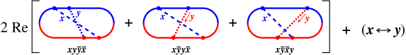
Figure 14: The sum of diagrams that define the quantity $A(x,y)$ in ref. 2brem .

6 Numerical results

6.1 Main results

To get results for $1/N^{2}$ corrections, we numerically integrated over $(t_{1},t_{2},\Delta t)$ or $(t_{1},\Delta t)$. A short discussion of our numerical method is given in appendix B. For comparison, the $N{=}\infty$ results from previous literature only require numerical integration over $\Delta t$. Dividing $1/N^{2}$ corrections by the corresponding $N{=}\infty$ result gives the relative size of the corrections.

The relative size of $1/N^{2}$ corrections to crossed and sequential diagrams for overlapping double splitting $g{\to}ggg$ are shown, respectively, in figs. 15 and 16 for $N{=}3$ (QCD). Our convention in these plots is to let $y$ represent the energy fraction of the lowest-energy daughter, $x$ represent the next lowest, and then $z=1{-}x{-}y$ represents the highest-energy daughter. So the plot region has been restricted by these conventions to $y<x<1{-}x{-}y$. The $1/N^{2}$ corrections to sequential diagrams are very small: less than 1%. The corrections to crossed diagrams are substantially larger. The largest relative correction occurs at the apex of the triangular region, $(x,y,z)=(\frac{1}{3},\frac{1}{3},\frac{1}{3})$, where the correction is roughly 17%.

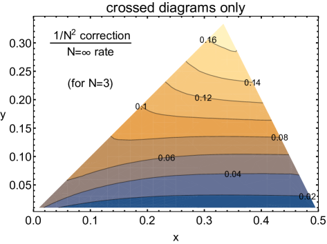
Figure 15: The ratio, for crossed diagrams only, of (i) the $1/N^{2}$ correction to (ii) the $N{=}\infty$ result for the differential rate $d\Gamma/dx\,dy$ for (the crossed diagram contribution to) overlapping double splitting $g\to ggg$. We have used $N{=}3$ in this plot, but one may multiply the results by $(3/N)^{2}$ to restore the $N$ dependence of the $1/N^{2}$ correction. Very tiny wiggles in the contour lines are an artifact of interpolation from a discrete set of numerical data points. We have left out $y<0.01$ just to simplify the numerical effort that went into making this plot. The ratio goes to zero as $y{\to}0$, as one may see from the later discussion of fig. 19 for a particular value of $x$.

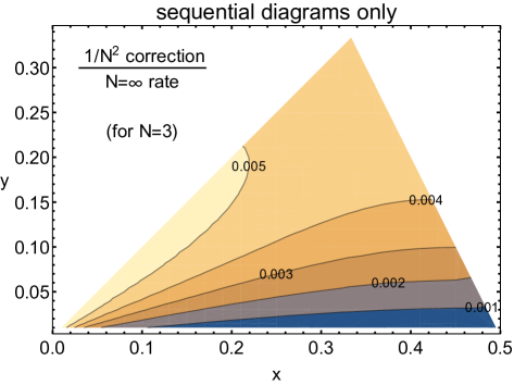
Figure 16: Like fig. 15 except now for sequential diagrams instead of crossed diagrams.

We showed the separate crossed and sequential diagram ratios first because there is a subtlety to discussing relative corrections to the total rate (crossed plus sequential). Fig. 17 shows a plot of the ratio

$$\frac{\mbox{total $1/N^{2}$ correction}}{\mbox{total $N{=}\infty$ rate}}$$ (108)

for $g\to ggg$, but restricted to $y>0.1$. Similar to fig. 15, there is a (local) maximum at the apex of the triangular region, where the $1/N^{2}$ correction is roughly 17%. Unlike fig. 15, however, around $y\sim 0.1$ the rate has started to grow with decreasing $y$. As we will explain, this small-$y$ growth is an artifact of how we have so far chosen to look at the size of $1/N^{2}$ corrections.

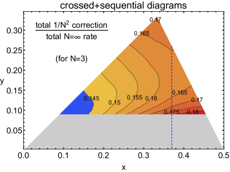
Figure 17: Like figs. 15 and 16 except now for the total $g\to ggg$ rate. The behavior for y<0.1 (the gray shaded region) is discussed in the main text.

Instead of showing the ratio (108), fig. 18 shows, for a particular value of $x$, the small-$y$ behavior of (i) the $N{=}\infty$ result for the total rate vs. (ii) the sum of the $N{=}\infty$ result and the $1/N^{2}$ correction. We’ve taken $x=0.37$, which corresponds to the blue dashed line in fig. 17. At small $y$, both the $N{=}\infty$ results and the total $1/N^{2}$ correction blow up as $1/y^{3/2}$, and so we have followed the convention of ref. seq and instead plotted

$$\pi^{2}xy^{3/2}\left[\Delta\frac{d\Gamma}{dx\,dy}\right]_{\rm total}$$ (109)

in fig. 18. The extremely tiny values of $y$ plotted in the figure are unlikely to ever be relevant to any real-world physics because, at the very least, one needs $yE\gg T$ for our high-energy approximations. Nonetheless, this figure is useful to understand the behavior of our formulas. The important feature is that the total $N{=}\infty$ result crosses zero at $y\sim 0.01$ (for this value of $x$). This is possible because $\Delta\Gamma/dx\,dy$ does not represent a rate; it represents the correction to a rate due to overlapping formation times (see section 1.1 of ref. seq for explanation), and a correction may be positive or negative. Where the $N{=}\infty$ result vanishes, the relative size (108) of the $1/N^{2}$ correction to that $N{=}\infty$ result will blow up to infinity, by definition. From fig. 18, however, one sees that there is very little difference between the $N{=}\infty$ curve and the corrected curve for $y<0.1$. In any case, in applications to energy loss and in-medium shower development, the $1/y^{3/2}$ small-$y$ behavior of overlapping double splitting $g{\to}ggg$ is canceled qcd by similar behavior of virtual corrections to single splitting $g{\to}gg$, leaving behind double-log divergences Blaizot ; Iancu ; Wu that are independent of $N$. So the small-$y$ behavior of fig. 18, and in particular the $1/N^{2}$ corrections to the small-$y$ behavior, are not of much physical interest. Furthermore, the original motivation for the large-$N$ approximation in this problem was as a tool to be able to study overlapping hard splittings ($y\sim x\sim 1$).

In principle, the best way to investigate the size of $1/N^{2}$ corrections would be to quote the relative size of their effect on an (infrared-safe) characteristic of in-medium shower development. Since we do not have everything needed for that (such as $1/N^{2}$ corrections for virtual diagrams), we interpret fig. 18 to mean that a reasonable proxy is the largest relative size of the $1/N^{2}$ corrections to $d\Gamma/dx\,dy$ for $y$ values that are not small — namely, the roughly 17% correction at the apex of fig. 17.

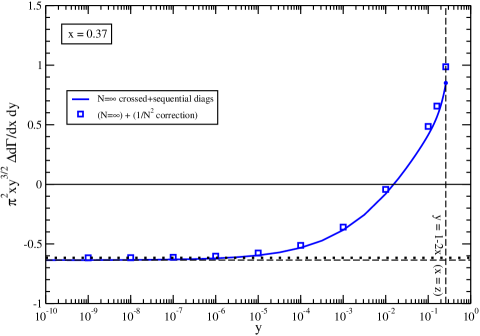
Figure 18: A plot for $x=0.37$ of the $y$ dependence of the total $\Delta\,d\Gamma/dx\,dy$, multiplied by $\pi^{2}xy^{3/2}$ [and in units of $N\alpha_{\rm s}\sqrt{\hat{q}_{\rm A}/E}$, but remember that $N\alpha_{\rm s}$ is held fixed as $N{\to}\infty$]. The plot shows (solid curve) the $N{=}\infty$ value and (squares) the $N{=}\infty$ value plus the $1/N^{2}$ correction. The horizontal dashed line shows the limiting $y{\to}0$ behavior of the $N{=}\infty$ result, and the nearby horizontal dotted line shows the limiting behavior of the corrected result.

6.2 More detail on small-$y$ behavior of crossed vs. sequential

There are some interesting qualitative features about the small-$y$ behavior of crossed vs. sequential diagrams. Fig. 19 shows various different elements that went into the previous small-$y$ numerics of fig. 18.

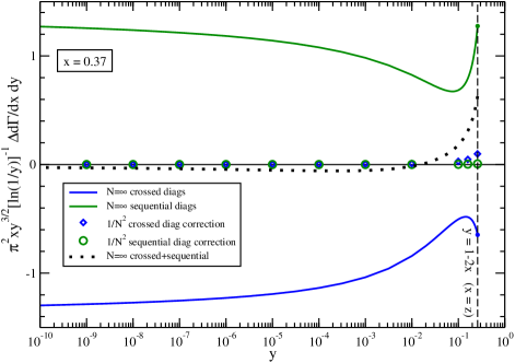
Figure 19: A plot for $x=0.37$ of the $y$ dependence of the different contributions to $\Delta\,d\Gamma/dx\,dy$, multiplied by $\pi^{2}xy^{3/2}$ and then divided by $\ln(y^{-1})$. The dotted line shows the total crossed+sequential $N{=}\infty$ result, corresponding to the solid curve in fig. 18. Note that the vertical axis is normalized differently here than in fig. 18, but still presented in units of $N\alpha_{\rm s}\sqrt{\hat{q}_{\rm A}/E}$. [The intended purpose of this plot is qualitative. See fig. 20 if interested in the precise values corresponding to the $1/N^{2}$ data points.]

First, as noted originally in ref. seq , the $N{=}\infty$ crossed and sequential results individually behave like $\ln(y^{-1})/y^{3/2}$ even though their sum just behaves like $1/y^{3/2}$. Because of the log dependence of the individual contributions, we have chosen to plot the contributions to

$$\frac{\pi^{2}xy^{3/2}}{\ln(y^{-1})}\,\left[\Delta\frac{d\Gamma}{dx\,dy}\right]$$ (110)

here instead of the normalization (109) used for fig. 18.

Notice that the absolute size of the $1/N^{2}$ correction to sequential diagrams (green circles in fig. 19) is quite small compared to that for crossed diagrams (blue diamonds). This means that, in absolute terms, the total $1/N^{2}$ correction is overwhelmingly dominated by crossed diagrams. [Sequential diagrams play a role in the size of relative corrections shown in fig. 17 because they affect the $N{=}\infty$ denominator of (108) even though they do not noticeably affect the $1/N^{2}$ numerator.]

Fig. 20, where the normalization of the verical axis is returned to (109), shows that the crossed and sequential $1/N^{2}$ corrections are different in another way as well. From this plot, we find numerically that the crossed diagram correction behaves like $1/y^{3/2}$ for small $y$, with no $\ln(y^{-1})$ enhancement. This is why the corresponding blue diamonds in fig. 19 approach zero, due to the additional normalization factor $1/\ln(y^{-1})$ in that plot. In contrast, we find that the sequential diagram correction has an even milder dependence on small $y$, behaving like $1/y^{1/2}$. When integrated over $y$ in applications, this means that the $1/N^{2}$ correction from crossed diagrams will contribute to infrared (IR) divergences (similar to the IR divergences of the $N{=}\infty$ results discussed in ref. qcd ), but the $1/N^{2}$ correction from sequential diagrams will be IR finite.

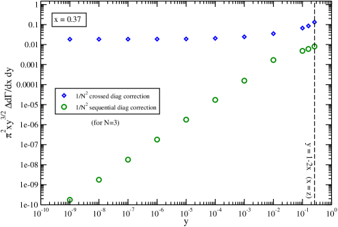
Figure 20: A plot for $x=0.37$ of the $y$ dependence of the different $1/N^{2}$ contributions to $\Delta\,d\Gamma/dx\,dy$, multiplied by $\pi^{2}xy^{3/2}$ as in fig. 18. Note that, in contrast to fig. 19, we have not divided by $\ln(1/y)$.

6.3 Comparison of size of $1/N^{2}$ corrections to related work

In this paper, we have been focused on the problem of overlapping formation times for the double splitting process $g{\to}ggg$. For simplicity, we have followed previous $N{=}\infty$ work on this problem 2brem ; seq ; qcd and only considered rates $\Delta\,d\Gamma/dx\,dy$ that have been integrated over the (small) transverse momenta ${\bm{p}}_{\perp}$ of all three daughters. For technical reasons, studying ${\bm{p}}_{\perp}$-integrated rates allows one to ignore what happens to any daughter after it has been emitted in both the amplitude and conjugate amplitude. It’s the reason, for example, why the dynamics of the $y$ gluon is no longer relevant after the first conjugate-amplitude (red) vertex in fig. 3 for $xy\bar{y}\bar{x}$ interference diagram.

However, there is a different type of problem (not about overlapping formation times) where similar issues of 4-gluon color-singlet dynamics also arise: the un-integrated ${\bm{p}}_{\perp}$ distribution $d\Gamma/dx\,d^{2}p_{\perp}$ for single splitting $g{\to}gg$ in the medium. Unlike fig. 1 for the ${\bm{p}}_{\perp}$-integrated $g{\to}gg$ rate, one must instead follow the color dynamics for a time after the splitting has taken place in both amplitude and conjugate amplitude, corresponding to the shaded region of fig. 21. During this time, one must treat the color dynamics of the four gluons shown in the shaded region. Refs. NSZ6j ; Zakharov6j ; Konrad have investigated how to treat this problem beyond the $N{=}\infty$ limit. Unlike our work (on our different problem), their calculations approximate the trajectories of the high-energy particles as perfectly straight lines. So they only include color dynamics and not the dynamics of particle trajectories. In this rigid geometry approximation (also known as the “antenna” approximation), they are able to more easily treat finite or expanding media.

Figure 21: Similar to fig. 1a for the rate of single splitting $g{\to}gg$, but here including later time-evolution of the daughters (shaded region) that must be included in order to study the ${\bm{p}}_{\perp}$ distribution of the daughters. In the shaded region, the above interference term contains four gluon lines which, in the language we have used in this paper, requires treating 4-gluon color singlet dynamics in the medium.

For our specific purposes here, ref. Konrad is interesting because the authors explicitly calculate the $1/N^{2}$ correction to the $N{=}\infty$ limit (using a different approach to calculate $1/N^{2}$ corrections than we have). In their numerics, they study a medium of length $L$ with constant $\hat{q}$. Their results will depend on $L$, and they study the case where the dimensionless ratio $L\sqrt{\hat{q}/E}$ (which parametrically is the ratio of $L$ to what the formation length $L_{\rm f}$ would be in an infinite medium) is $\simeq 0.55$. In this particular case, they find that the $1/N^{2}$ correction to the $N{=}\infty$ distribution for $g{\to}gg$ can be as large as 16%. Direct comparison to our roughly 17% correction should not be taken too seriously, however, since (i) the process we study is very different, and (ii) their numerics hold quark $\hat{q}_{\rm F}$ fixed as they vary $N$, whereas we hold gluon $\hat{q}_{\rm A}$ fixed.

7 Conclusion

With two caveats, we have found that $1/N^{2}$ corrections to $N{=}\infty$ results for overlapping double gluon splitting ($g\to ggg$) can be as large as approximately 17% for $N{=}3$ (QCD). One caveat is the technical one explained in section 6.1 that measurements of relative corrections become meaningless when the leading ($N{=}\infty$) answer goes through zero at small $y\sim 0.01$, and so we have focused on the size of corrections for not-small $y$. Also, small-$y$ emission is not the case where large-$N$ techniques were necessary to simplify the problem, since previous work on overlapping formation times with a soft emission Blaizot ; Iancu ; Wu (which included the effects of virtual emissions) was done without resorting to the large-$N$ approximation. Our interest here has been to estimate the reliability of using $N{=}\infty$ results specifically for the case where $y$ is not small.

The other caveat is that, in this exploratory analysis, we have not included diagrammatic contributions to $g{\to}ggg$ that involve 4-gluon vertices nor, in Light-Cone Perturbation Theory, instantaneous longitudinal gluon exchange. Nonetheless, our provisional take-away is that the $N{=}\infty$ limit taken in previous analysis is likely a moderately good approximation. Work on using the $N{=}\infty$ approximation to answer the ultimate question about the effect of overlapping non-soft emission on in-medium shower development is ongoing (using results for $N{=}\infty$ rates from ref. qcd and the framework suggested by ref. qedNfstop ).

Ultimately, a complete analysis of $1/N^{2}$ effects on energy loss should also include calculation of virtual diagrams for $g\to gg$, as discussed for $N{=}\infty$ in ref. qcd .

Calculating virtual diagrams through order $1/N^{2}$ may also be interesting for better understanding soft radiative corrections to hard single splitting $g{\to gg}$. Such radiative corrections give rise to IR double logarithms Blaizot ; Iancu ; Wu and sub-leading IR single logarithms. The single logarithms have been calculated for $N{=}\infty$ (for infinite medium in the $\hat{q}$ approximation) in refs. logs ; logs2 . We do not know for sure whether those single logarithms have any non-trivial dependence on $N$. It would be interesting to be able to explicitly check at order $1/N^{2}$.

Finally, to answer a question proposed in the introduction, we note that our roughly 17% corrections for $N{=}3$ are roughly consistent with (e.g. within a factor of 2 of) the naive, merely parametric guess of $O(1/N^{2})\sim 10\%$.

Appendix A More on $(s,t,u)$ channel color singlet states

A.1 Sign conventions and conversions

The overall sign conventions for $u$-channel states in this paper were set by how we translated the $s$-channel results for the potential $V({\bm{C}}_{12},{\bm{C}}_{34})$ in eqs. (4.3) and (3.12a) of ref. color to the $u$-channel version shown here in (8). The translation is to simply relabel the particles $(1,2,3,4)$ there as $(4,1,2,3)$ here. We take our basis of color states (7) to be similarly permuted:

$$(1,2,3,4)\longrightarrow(4,1,2,3)\qquad\mbox{[for $s\to u$]}$$ (111)

to go from $s$-channel $|R\rangle_{s}$ to $u$-channel $|R\rangle_{u}$. Because we have used the same permutation to define our $u$-channel states, our formulas (10) here for the matrices $\underline{S}_{u}$ and $\underline{T}_{u}$ are the same as the corresponding $s$-channel versions in eq. (5.6) of ref. color .

However, (111) is not how $u$-channel states were defined in ref. color . There, $t$-channel states were first defined by

$$2\leftrightarrow 3\qquad\mbox{[for $s\to t$]},$$ (112)

and then $u$-channel states were defined in terms of $t$-channel states by

$$3\leftrightarrow 4\qquad\mbox{[for $t\to\bar{u}$]},$$ (113)

where we will use $\bar{u}$ to denote the $u$-channel conventions of ref. color . Performing (112) followed by (113) gives

$$(1,2,3,4)\longrightarrow(1,4,2,3)\qquad\mbox{[for $s\to\bar{u}$]}$$ (114)

The difference between our $u$-channel convention on the right-hand side of (111) and the convention on the right-hand side of (114) is

$$1\leftrightarrow 4\qquad\mbox{[for $u\to\bar{u}$]},$$ (115)

The effect of this is to negate states that involves an anti-symmetric combination of particles 1 and 4. From (6), that’s $|{\rm A}_{aa}\rangle_{u}$ and $|``\bm{10}+\overline{\bm{10}}"\rangle_{u}$ out of our $u$-channel states (7). We can summarize this as

$$\begin{pmatrix}|{\bm{1}}\rangle_{\bar{u}}\\ |{\rm A}_{\rm aa}\rangle_{\bar{u}}\\ |{\rm A}_{\rm ss}\rangle_{\bar{u}}\\ |``\bm{10}{+}\overline{\bm{10}}"\rangle_{\bar{u}}\\ |``\bm{27}"\rangle_{\bar{u}}\\ |``\bm{0}"\rangle_{\bar{u}}\end{pmatrix}=\mathds{P}\begin{pmatrix}|{\bm{1}}\rangle_{u}\\ |{\rm A}_{\rm aa}\rangle_{u}\\ |{\rm A}_{\rm ss}\rangle_{u}\\ |``\bm{10}{+}\overline{\bm{10}}"\rangle_{u}\\ |``\bm{27}"\rangle_{u}\\ |``\bm{0}"\rangle_{u}\end{pmatrix}\qquad\mbox{with}\qquad\mathds{P}\equiv\begin{pmatrix}+1&&&&&\\ &-1&&&&\\ &&+1&&&\\ &&&-1&&\\ &&&&+1&\\ &&&&&+1\\ \end{pmatrix}.$$ (116)

The matrix that converts (for any $N$) between $s$-channel and $t$-channel versions of the original basis states is given by refs. color ; NSZ6j ; Sjodahl as

$$\begin{pmatrix}|{\bm{1}}\rangle_{s}\\ |{\rm A}_{\rm aa}\rangle_{s}\\ |{\rm A}_{\rm ss}\rangle_{s}\\ |``\bm{10}{+}\overline{\bm{10}}"\rangle_{s}\\ |``\bm{27}"\rangle_{s}\\ |``\bm{0}"\rangle_{s}\end{pmatrix}=\mathds{V}\begin{pmatrix}|{\bm{1}}\rangle_{t}\\ |{\rm A}_{\rm aa}\rangle_{t}\\ |{\rm A}_{\rm ss}\rangle_{t}\\ |``\bm{10}{+}\overline{\bm{10}}"\rangle_{t}\\ |``\bm{27}"\rangle_{t}\\ |``\bm{0}"\rangle_{t}\end{pmatrix}$$ (117)

with

$$\mathds{V}=\begin{pmatrix}\tfrac{1}{N^{2}-1}&\sqrt{\tfrac{1}{N^{2}-1}}&\sqrt{\tfrac{1}{N^{2}-1}}&\sqrt{\tfrac{N^{2}-4}{2(N^{2}-1)}}&\tfrac{N}{2(N+1)}\sqrt{\tfrac{N+3}{N-1}}&\tfrac{N}{2(N-1)}\sqrt{\tfrac{N-3}{N+1}}\\[5.0pt] &\tfrac{1}{2}&\tfrac{1}{2}&0&-\tfrac{1}{2}\sqrt{\tfrac{N+3}{N+1}}&\tfrac{1}{2}\sqrt{\tfrac{N-3}{N-1}}\\ &&\tfrac{N^{2}-12}{2(N^{2}-4)}&-\sqrt{\tfrac{2}{N^{2}-4}}&\tfrac{N}{2(N+2)}\sqrt{\tfrac{N+3}{N+1}}&-\tfrac{N}{2(N-2)}\sqrt{\tfrac{N-3}{N-1}}\\[5.0pt] &&&\tfrac{1}{2}&-\sqrt{\tfrac{(N-2)(N+3)}{8(N+1)(N+2)}}&-\sqrt{\tfrac{(N+2)(N-3)}{8(N-1)(N-2)}}\\[5.0pt] \lx@intercol\hfil\rm(symmetric)\hfil\lx@intercol&&\tfrac{N^{2}+N+2}{4(N+1)(N+2)}&\tfrac{1}{4}\sqrt{\tfrac{N^{2}-9}{N^{2}-1}}\\[5.0pt] &&&&&\tfrac{N^{2}-N+2}{4(N-1)(N-2)}\\ \end{pmatrix}.$$ (118)

(Note that $\mathds{V}=\mathds{V}^{\top}=\mathds{V}^{-1}$.) As explained in ref. color , the conversion between the $s$-channel and the $u$-channel basis of that paper is correspondingly

$$\begin{pmatrix}|{\bm{1}}\rangle_{s}\\ |{\rm A}_{\rm aa}\rangle_{s}\\ |{\rm A}_{\rm ss}\rangle_{s}\\ |``\bm{10}{+}\overline{\bm{10}}"\rangle_{s}\\ |``\bm{27}"\rangle_{s}\\ |``\bm{0}"\rangle_{s}\end{pmatrix}=\mathds{P}\mathds{V}\begin{pmatrix}|{\bm{1}}\rangle_{\bar{u}}\\ |{\rm A}_{\rm aa}\rangle_{\bar{u}}\\ |{\rm A}_{\rm ss}\rangle_{\bar{u}}\\ |``\bm{10}{+}\overline{\bm{10}}"\rangle_{\bar{u}}\\ |``\bm{27}"\rangle_{\bar{u}}\\ |``\bm{0}"\rangle_{\bar{u}}\end{pmatrix}.$$ (119)

Using (116), the conversion between the $s$-basis and $u$-basis in our paper here is given by (79a) with $\mathds{U}=\mathds{P}\mathds{V}\mathds{P}$, which equals (79b). For some purposes, it is useful to have the $N{=}\infty$ limit of this matrix, which is

$$\mathds{U}^{N=\infty}=\begin{pmatrix}0&0&0&-\tfrac{1}{\sqrt{2}}&\tfrac{1}{2}&\tfrac{1}{2}\\[3.0pt] 0&\tfrac{1}{2}&-\tfrac{1}{2}&0&\tfrac{1}{2}&-\tfrac{1}{2}\\[3.0pt] 0&-\tfrac{1}{2}&\tfrac{1}{2}&0&\tfrac{1}{2}&-\tfrac{1}{2}\\[3.0pt] -\tfrac{1}{\sqrt{2}}&0&0&\tfrac{1}{2}&\tfrac{1}{2\sqrt{2}}&\tfrac{1}{2\sqrt{2}}\\[3.0pt] \tfrac{1}{2}&\tfrac{1}{2}&\tfrac{1}{2}&\tfrac{1}{2\sqrt{2}}&\tfrac{1}{4}&\tfrac{1}{4}\\[3.0pt] \tfrac{1}{2}&-\tfrac{1}{2}&-\tfrac{1}{2}&\tfrac{1}{2\sqrt{2}}&\tfrac{1}{4}&\tfrac{1}{4}\end{pmatrix}.$$ (120)

A.2 Alternative descriptions for $N{=}\infty$

Here, we will justify the $N{=}\infty$ identifications made in (15). One relatively simple method is to start with a form where the potential $V$ is written directly in terms of the transverse positions $({\bm{b}}_{1},{\bm{b}}_{2},{\bm{b}}_{3},{\bm{b}}_{4})$ of the four individual particles instead of in terms of reduced variables such as the $({\bm{C}}_{41},{\bm{C}}_{23})$ of (8b). This more direct expression is color

$$\underline{V}({\bm{b}}_{1},{\bm{b}}_{2},{\bm{b}}_{3},{\bm{b}}_{4})=\frac{i\hat{q}_{\rm A}}{4C_{\rm A}}\biggl{\{} \underline{{\mathbb{T}}}_{1}\cdot\underline{{\mathbb{T}}}_{2}\bigl{[}({\bm{b}}_{1}{-}{\bm{b}}_{2})^{2}+({\bm{b}}_{3}{-}{\bm{b}}_{4})^{2}\bigr{]}$$

$$+\underline{{\mathbb{T}}}_{1}\cdot\underline{{\mathbb{T}}}_{3}\bigl{[}({\bm{b}}_{1}{-}{\bm{b}}_{3})^{2}+({\bm{b}}_{2}{-}{\bm{b}}_{4})^{2}\bigr{]}$$

$$+\underline{{\mathbb{T}}}_{1}\cdot\underline{{\mathbb{T}}}_{4}\bigl{[}({\bm{b}}_{1}{-}{\bm{b}}_{4})^{2}+({\bm{b}}_{2}{-}{\bm{b}}_{3})^{2}\bigr{]}\biggr{\}}.$$ (121)

(This expression only assumes the $\hat{q}$ approximation and not that the medium is itself weakly coupled.) Now we can use the expressions (9) for the $\underline{{\mathbb{T}}}_{i}\cdot\underline{{\mathbb{T}}}_{j}$ in terms of $\underline{S}_{u}$ and $\underline{T}_{u}$. Then remember that for $N{=}\infty$ our basis states $(1,{\rm A}_{+},{\rm A}_{-},{\rm A}^{\!\times},1^{\times}_{+},1^{\times}_{-})$ are simultaneous eigenstates of $\underline{S}_{u}$ and $\underline{T}_{u}$ with eigenvalues given by the corresponding diagonal entries of (14). All together, we can then write the explicit 4-particle potential for each of our basis states.

For example, for $|{\rm A}_{-}\rangle$, eq. (14) indicates that $(S_{u},T_{u})=(\frac{1}{2},-\frac{1}{4})$ for $N{=}\infty$. Using (9), the corresponding potential (121) is then

$$V^{N=\infty}_{({\rm A}_{-})}({\bm{b}}_{1},{\bm{b}}_{2},{\bm{b}}_{3},{\bm{b}}_{4})=-\frac{i{\hat{q}}_{\rm A}}{8}\Bigl{[}({\bm{b}}_{1}{-}{\bm{b}}_{2})^{2}+({\bm{b}}_{2}{-}{\bm{b}}_{3})^{2}+({\bm{b}}_{3}{-}{\bm{b}}_{4})^{2}+({\bm{b}}_{4}{-}{\bm{b}}_{1})^{2}\Bigr{]}.$$ (122)

This is exactly the large-$N$ behavior that we characterized as “(1234),” where each particle can interact only with its neighbors going around the cylinder.

Doing the same thing with $|{\rm A}^{\!\times}\rangle$, which has $(S_{u},T_{u})=(0,0)$ for $N{=}\infty$, gives

$$V^{N=\infty}_{({\rm A}^{\!\times})}({\bm{b}}_{1},{\bm{b}}_{2},{\bm{b}}_{3},{\bm{b}}_{4})=-\frac{i{\hat{q}}_{\rm A}}{8}\Bigl{[}({\bm{b}}_{1}{-}{\bm{b}}_{2})^{2}+({\bm{b}}_{2}{-}{\bm{b}}_{4})^{2}+({\bm{b}}_{4}{-}{\bm{b}}_{3})^{2}+({\bm{b}}_{3}{-}{\bm{b}}_{1})^{2}\Bigr{]},$$ (123)

which corresponds to what we called (1243).

As another example, $|1^{\times}_{-}\rangle$ has $(S_{u},T_{u})=(0,-\frac{1}{2})$ for $N{=}\infty$, which gives

$$V^{N=\infty}_{(1^{\times}_{-})}({\bm{b}}_{1},{\bm{b}}_{2},{\bm{b}}_{3},{\bm{b}}_{4})=-\frac{i{\hat{q}}_{\rm A}}{4}\Bigl{[}({\bm{b}}_{1}{-}{\bm{b}}_{2})^{2}+({\bm{b}}_{3}{-}{\bm{b}}_{4})^{2}\Bigr{]},$$ (124)

where particles 1 and 2 interact only with each other, and similarly particles 3 and 4 interact only with each other. This corresponds to what we called $(12)(34)$. One may similarly check all of the other identifications in (15).

Appendix B Numerical method

Here, we give a few comments about our numerical method. We have not tried to figure out the most efficient method but have adopted a brute-force approach implemented in Mathematica Mathematica . But there are issues, which we think may be useful to briefly summarize.

First, because of round-off errors caused by subtractive cancellations, we find that we typically need to do intermediate calculations with much more than machine precision in order to succeed in a brute force approach. We therefore do our calculations with higher precision arithmetic in Mathematica.

Some of our formulas, like (51), involve derivatives such as $\partial_{j_{1}}\partial_{j_{2}}[\cdots]\Bigl{|}_{j_{1}=j_{2}=0}$. After some experimentation, we decided to implement these derivatives numerically as

$$\partial_{j_{1}}\partial_{j_{2}}f(j_{1},j_{2})\Bigl{|}_{j_{1}=j_{2}=0}\simeq\frac{f({+}\epsilon,{+}\epsilon)-f({+}\epsilon,{-}\epsilon)-f({-}\epsilon,{+}\epsilon)+f({-}\epsilon,{-}\epsilon)}{(2\epsilon)^{2}}\qquad\mbox{($\epsilon$ small)}$$ (125)

rather than doing the derivatives analytically (or using a more sophisticated numerical estimate of the derivative).

We let Mathematica handle the numerical evaluation of matrix inverses and determinants in our formulas.

We found that naive use of canned, adaptive integration routines took too much CPU time and caused a host of problems. Rather than working out how to tweak adaptive integration to do what we needed, we just did all of our integrals as simply as possible by using midpoint Riemann sums. For the $\Delta t$ integral (as opposed to the $t_{1}$ and $t_{2}$ integrals), we found it convenient to change variables as $\int_{0}^{\infty}d(\Delta t)\>f(\Delta t)=\int_{-\infty}^{\infty}dz\>e^{z}f(e^{z}).$ In practice, we then replace the infinite $z$ integration region $(-\infty,+\infty)$ by a finite region $(z_{\rm min},z_{\rm max})$ carefully chosen to cover everywhere the integrand is non-negligible [a choice which must be adjusted to study small values of $y$].

The cost of our brute-force method is that, because it is not adaptive, there are an annoying number of numerical approximations one must check to be sure that results are accurate, e.g. the size of $\epsilon$ in the numerical derivatives, the number of Riemann intervals for the $(t_{1},t_{2},z)$ integrals, and the cut-offs $(z_{\rm min},z_{\rm max})$.

Finally, we should mention the strategies we used to attempt to avoid human error in our analysis and coding. The result (41) for the $1/N^{2}$ correction $\delta^{2}G$ to the 4-particle propagator was initially derived independently, and implemented numerically, by each of us in very different ways. One way was the method presented in the text. The other way did not use any tricks for packaging the transverse-position integrations into higher-dimensional vectors and matrices like eqs. (21), (36) and (39) but instead did the Gaussian integrals separately and explicitly, resulting in very long mathematical expressions for $\delta^{2}G$. Once the two methods agreed numerically, we then both switched to the method and code that most quickly produced results for $\delta^{2}G$, which was the method based on (41). Now using the same code for $\delta^{2}G$, we each independently produced or spot checked the various results in this paper. Since we consulted with each other on general methods and development [e.g. equations like (46)], and helped each other to ferret out sources of numerical discrepancy, our work was not completely independent, but the most error-prone aspects of our numerical work were done independently.

References

- (1) L. D. Landau and I. Pomeranchuk, “Limits of applicability of the theory of bremsstrahlung electrons and pair production at high-energies,” Dokl. Akad. Nauk Ser. Fiz. 92 (1953) 535.
- (2) L. D. Landau and I. Pomeranchuk, “Electron cascade process at very high energies,” Dokl. Akad. Nauk Ser. Fiz. 92 (1953) 735.
- (3) A. B. Migdal, “Bremsstrahlung and pair production in condensed media at high-energies,” Phys. Rev. 103, 1811 (1956);
- (4) L. Landau, The Collected Papers of L.D. Landau (Pergamon Press, New York, 1965).
- (5) R. Baier, Y. L. Dokshitzer, A. H. Mueller, S. Peigne and D. Schiff, “The Landau-Pomeranchuk-Migdal effect in QED,” Nucl. Phys. B 478, 577 (1996) [arXiv:hep-ph/9604327];
- (6) R. Baier, Y. L. Dokshitzer, A. H. Mueller, S. Peigne and D. Schiff, “Radiative energy loss of high-energy quarks and gluons in a finite-volume quark-gluon plasma,” Nucl. Phys. B 483, 291 (1997) [arXiv:hep-ph/9607355].
- (7) R. Baier, Y. L. Dokshitzer, A. H. Mueller, S. Peigne and D. Schiff, “Radiative energy loss and -broadening of high energy partons in nuclei,” Nucl. Phys. B 484 (1997) [arXiv:hep-ph/9608322].
- (8) R. Baier, Y. L. Dokshitzer, A. H. Mueller and D. Schiff, “Medium induced radiative energy loss: Equivalence between the BDMPS and Zakharov formalisms,” Nucl. Phys. B 531, 403-425 (1998) [arXiv:hep-ph/9804212 [hep-ph]].
- (9) B. G. Zakharov, “Fully quantum treatment of the Landau-Pomeranchuk-Migdal effect in QED and QCD,” JETP Lett. 63, 952 (1996) [arXiv:hep-ph/9607440].
- (10) B. G. Zakharov, “Radiative energy loss of high-energy quarks in finite size nuclear matter and quark-gluon plasma,” JETP Lett. 65, 615 (1997) [Pisma Zh. Eksp. Teor. Fiz. 63, 952 (1996)] [arXiv:hep-ph/9704255].
- (11) B. G. Zakharov, “Light cone path integral approach to the Landau-Pomeranchuk-Migdal effect,” Phys. Atom. Nucl. 61, 838-854 (1998) [arXiv:hep-ph/9807540 [hep-ph]].
- (12) J. P. Blaizot and Y. Mehtar-Tani, “Renormalization of the jet-quenching parameter,” Nucl. Phys. A 929, 202 (2014) [arXiv:1403.2323 [hep-ph]].
- (13) E. Iancu, “The non-linear evolution of jet quenching,” JHEP 10, 95 (2014) [arXiv:1403.1996 [hep-ph]].
- (14) B. Wu, “Radiative energy loss and radiative -broadening of high-energy partons in QCD matter,” JHEP 12, 081 (2014) [arXiv:1408.5459 [hep-ph]].
- (15) T. Liou, A. H. Mueller and B. Wu, “Radiative -broadening of high-energy quarks and gluons in QCD matter,” Nucl. Phys. A 916, 102 (2013) [arXiv:1304.7677 [hep-ph]].
- (16) P. Arnold and S. Iqbal, “The LPM effect in sequential bremsstrahlung,” JHEP 04, 070 (2015) [erratum JHEP 09, 072 (2016)] [arXiv:1501.04964 [hep-ph]].
- (17) P. Arnold, S. Iqbal and T. Rase, “Strong- vs. weak-coupling pictures of jet quenching: a dry run using QED,” JHEP 05, 004 (2019) [arXiv:1810.06578 [hep-ph]].
- (18) P. Arnold, H. C. Chang and S. Iqbal, “The LPM effect in sequential bremsstrahlung 2: factorization,” JHEP 09, 078 (2016) [arXiv:1605.07624 [hep-ph]].
- (19) P. Arnold, H. C. Chang and S. Iqbal, “The LPM effect in sequential bremsstrahlung: dimensional regularization,” JHEP 10, 100 (2016) [arXiv:1606.08853 [hep-ph]].
- (20) P. Arnold and S. Iqbal, “In-medium loop corrections and longitudinally polarized gauge bosons in high-energy showers,” JHEP 12, 120 (2018) [arXiv:1806.08796 [hep-ph]].
- (21) P. Arnold, T. Gorda and S. Iqbal, “The LPM effect in sequential bremsstrahlung: nearly complete results for QCD,” JHEP 11, 053 (2020) [arXiv:2007.15018 [hep-ph]].
- (22) P. Arnold, “Landau-Pomeranchuk-Migdal effect in sequential bremsstrahlung: From large- QCD to =3 via the SU() analog of Wigner 6- symbols,” Phys. Rev. D 100, no. 3, 034030 (2019) [arXiv:1904.04264 [hep-ph]].
- (23) N. N. Nikolaev, W. Schafer and B. G. Zakharov, “Nonlinear factorization for gluon-gluon dijets produced off nuclear targets,” Phys. Rev. D 72, 114018 (2005) [hep-ph/0508310].
- (24) B. G. Zakharov, “Color randomization of fast gluon-gluon pairs in the quark-gluon plasma,” J. Exp. Theor. Phys. 128, no.2, 243-258 (2019) [arXiv:1806.04723 [hep-ph]].
- (25) P. Arnold, H. C. Chang and S. Iqbal, “The LPM effect in sequential bremsstrahlung: 4-gluon vertices,” JHEP 10, 124 (2016) [arXiv:1608.05718 [hep-ph]].
- (26) P. Arnold, “Multi-particle potentials from light-like Wilson lines in quark-gluon plasmas: a generalized relation of in-medium splitting rates to jet-quenching parameters ,” Phys. Rev. D 99, no. 5, 054017 (2019) [arXiv:1901.05475 [hep-ph]].
- (27) M. Sjodahl and J. Thorén, “Decomposing color structure into multiplet bases,” JHEP 1509, 055 (2015) [arXiv:1507.03814 [hep-ph]].
- (28) L. M. Kaplan and M. Resnikoff, “Matrix Products and the Explit 3, 6, 9, and 12- Coefficients of the Regular Representation of . J. Math. Phys. 8, 2194 (1967).
- (29) R. P. Bickerstaff, P. H. Butler, M. B. Butts, R. W. Haase and M. F. Reid, “ and tables for some bases of SU6 and SU3,” J. Phys. A 15, 1087 (1982).
- (30) H. Elvang, P. Cvitanović and A. D. Kennedy, “Diagrammatic Young projection operators for U(n),” hep-th/0307186.
- (31) P. Cvitanović, Group theory: Birdtracks, Lie’s, and Exceptional Groups (Princeton University Press, 2008), also avaiable at http://birdtracks.eu/version9.0/GroupTheory.pdf.
- (32) G. ’t Hooft, “A Planar Diagram Theory for Strong Interactions,” Nucl. Phys. B 72, 461 (1974)
- (33) S. Coleman, Aspects of Symmetry: Selected Erice Lectures (Cambridge University Press, 1985).
- (34) J. H. Isaksen and K. Tywoniuk, “Wilson line correlators beyond the large-Nc,” JHEP 11, 125 (2021) [arXiv:2107.02542 [hep-ph]].
- (35) P. Arnold, T. Gorda and S. Iqbal, “The LPM effect in sequential bremsstrahlung: analytic results for sub-leading (single) logarithms,” [arXiv:2112.05161 [hep-ph]].
- (36) P. Arnold, “Universality (beyond leading log) of soft radiative corrections to in broadening and energy loss,” [arXiv:2111.05348 [hep-ph]].
- (37) Wolfram Research, Inc., Mathematica (various versions), Champaign, IL (2018–2021)