Quark and gluon form factors in four-loop QCD

Abstract

We compute the photon-quark and Higgs-gluon form factors to four-loop order within massless perturbative Quantum Chromodynamics. Our results constitute ready-to-use building blocks for N⁴LO cross sections for Drell-Yan processes and gluon-fusion Higgs boson production at the LHC. We present complete analytic expressions for both form factors and show several of the most complicated master integrals.

Introduction. A number of experimental results obtained at the Large Hadron Collider (LHC) at CERN have reached a precision below the percent level, often superseding the original expectations. A fundamental ingredient to the successful interpretation of precise data is the computation of higher order quantum corrections, most importantly those stemming from the strong interaction. In many cases next-to-next-to-leading order (NNLO) corrections have become standard. In fact, nowadays $2\to 2$ scattering processes are routinely computed at this order, in some cases even taking into account massive particles in the loops. Also for $2\to 3$ processes more and more results become available (see, e.g., Refs. [1, 2, 3, 4, 5, 6, 7]).

There are a few processes which are known to third order, or N³LO, in perturbative Quantum Chromodynamics (QCD). Among them are the Drell-Yan production of $W$ and $Z$ bosons [8, 9] as well as Higgs boson production in gluon fusion in the infinite top-mass limit [10, 11] at the LHC. In the latter case the high-order corrections are particularly important due to the slow convergence of the perturbative series. Similar observations have been made for the threshold production cross section of the top quark pairs in electron positron annihilation, where third-order corrections are necessary to obtain theory uncertainties of a few percent [12]. For more generic $2\to 2$ processes like dijet production, virtual corrections at third order QCD became available only recently, (see, e.g., Refs. [13, 14]), providing first ingredients to such N³LO cross sections.

In the coming years the precise determination of the Higgs boson properties will be one of the central topics at the LHC. In this context it is important to improve the precision for the production cross section, both experimentally and from the theory side. First steps towards the N⁴LO corrections of the Higgs boson production cross section have been undertaken in Ref. [15]. In this Letter we provide the first ready-to-use ingredient to the N⁴LO cross section for $gg\to H+X$ by presenting the virtual corrections to the effective Higgs-gluon vertex up to four-loop order. Similarly, we provide the four-loop corrections to the photon-quark vertex which are a building block of the N⁴LO corrections to the process $q\bar{q}\to Z/W$. Historically, also at N³LO the purely virtual corrections were the first building blocks to become available with the calculation of the three-loop form factors more than a decade ago [16, 17, 18]. Subsequently, the real-radiation contributions have been added step-by-step until first results for the Higgs production cross section became available [19, 20, 21, 22, 23, 24, 25].

The relevant form factors for the $q\bar{q}\gamma^{\ast}$ and $ggH$ vertex functions $\Gamma^{\mu}_{q}$ and $\Gamma^{\mu\nu}_{g}$, respectively, are given by the projections

$$F_{q}(q^{2}) =-\frac{1}{4(1-\epsilon)q^{2}}\mbox{Tr}\left(q_{2}\!\!\!\!\!/\,\,\,\Gamma^{\mu}q_{1}\!\!\!\!\!/\,\,\,\gamma_{\mu}\right)\,,$$ (1)

$$F_{g}(q^{2}) =\frac{\left(q_{1}\cdot q_{2}\,\,g_{\mu\nu}-q_{1,\mu}\,q_{2,\nu}-q_{1,\nu}\,q_{2,\mu}\right)}{2(1-\epsilon)}\Gamma^{\mu\nu}_{g}\,.$$ (2)

Here, the overall normalization is chosen such that both form factors are one at leading order. We employ conventional dimensional regularization and use $\epsilon=(4-d)/2$, where $d$ is the space-time dimension. The outgoing momentum of the photon (Higgs) is $q=q_{1}+q_{2}$, where $q_{1}$ and $q_{2}$ are the incoming momenta of the quark and anti-quark (gluons) for $F_{q}$ ($F_{g}$), and we have $q_{1}^{2}=q_{2}^{2}=0$ and $q^{2}\not=0$.

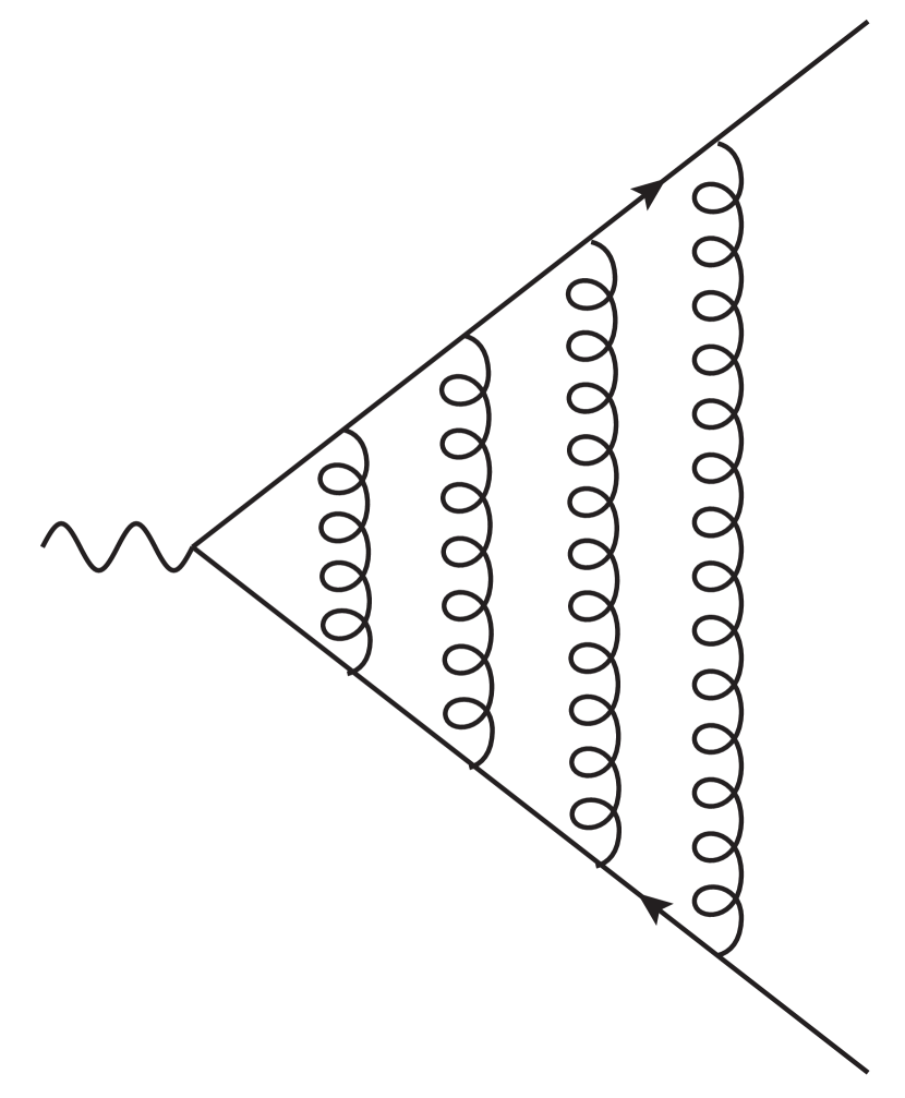
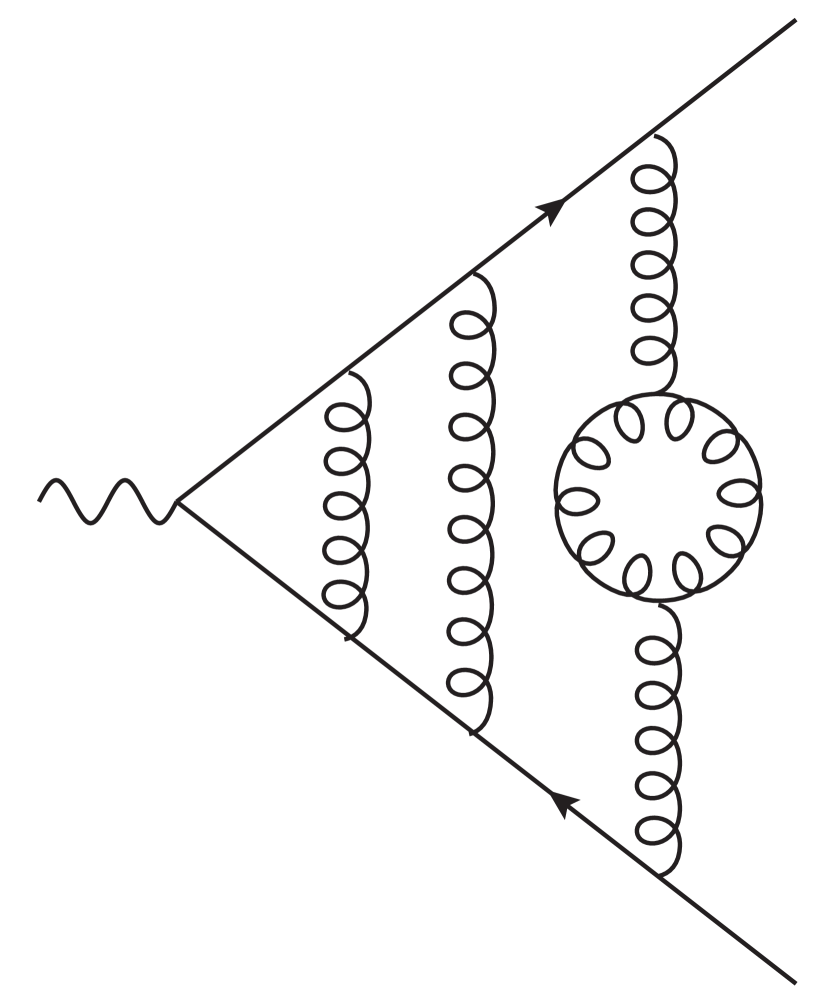
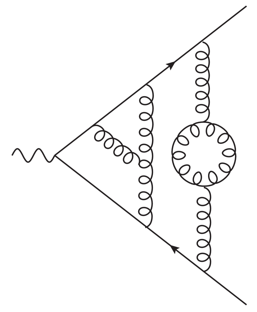
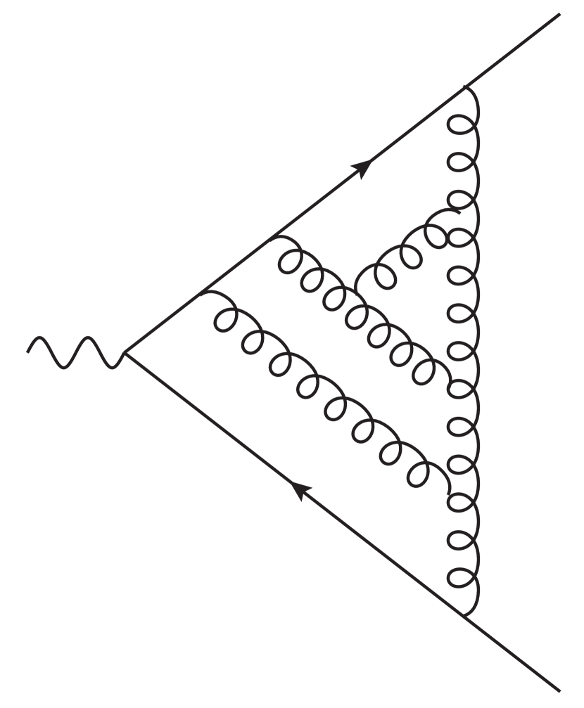
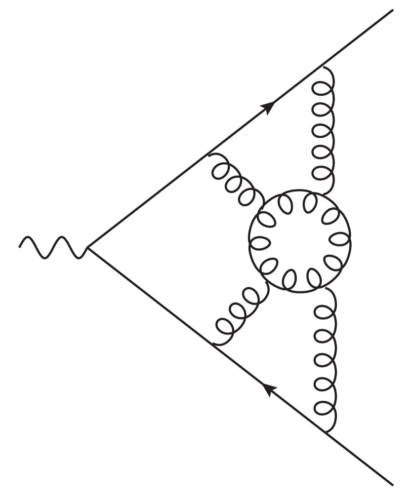
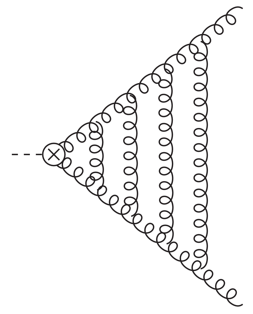
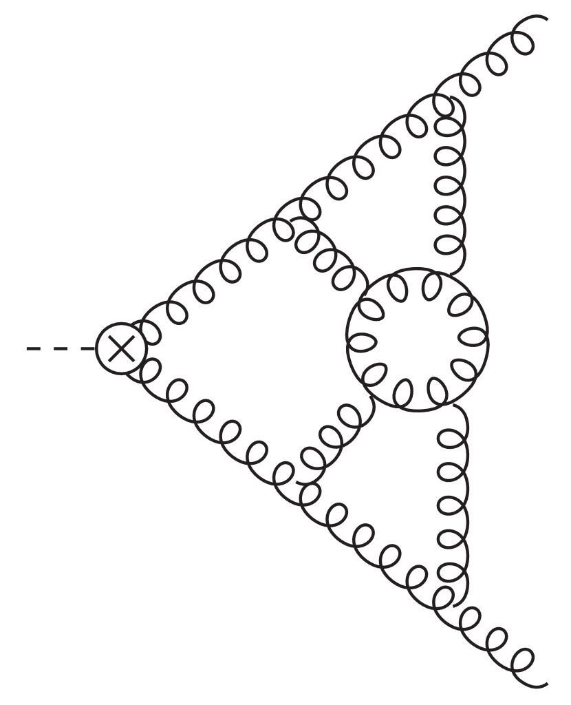
$F_{q}:\!\!$ $C_{F}^{4}$ $C_{F}^{3}C_{A}$ $C_{F}^{2}C_{A}^{2}$ $C_{F}C_{A}^{3}$ $d_{F}^{abcd}d_{A}^{abcd}$ $F_{g}:\!\!$ $C_{A}^{4}$ $d_{A}^{abcd}d_{A}^{abcd}$

Figure 1: Sample Feynman diagrams and color factors for the non-fermionic contributions to $F_{g}$ and $F_{q}$ at four-loop order. Straight and curly lines denote quarks and gluons, respectively. Both planar and non-planar diagrams contribute.

The two- and three-loop QCD corrections to $F_{q}$ and $F_{g}$ are available from Refs. [26, 27, 28, 29, 30, 16, 31, 16, 18, 32, 33, 34], At four loops, only partial results have been obtained so far. In Fig. 1 we show sample Feynman diagrams for the purely gluonic corrections to $F_{q}$ and $F_{g}$ in four-loop QCD; sample diagrams for the fermionic part can be found in Fig. 1 of Ref. [35]. Altogether 5728 and 43220 Feynman diagrams contribute to the quark and gluon form factor at this perturbative order, respectively.

The results, which are presented in this Letter, finalize a long-running effort to compute QCD form factors to four loops. First results have been obtained in 2016 [36, 37] where planar diagrams for $F_{q}$ have been presented in the large-$N_{c}$ limit. Fermionic corrections with two closed fermion bubbles are available from [38] and the complete contribution from color structure $(d_{F}^{abcd})^{2}$ has been computed in [39, 40]. For $F_{q}$ and $F_{g}$, all corrections with three or two closed fermion loops have been calculated in [41, 42], respectively, including also the singlet contributions. The complete set of poles of $F_{q}$ and $F_{g}$ in the dimensional regulator has been obtained through direct diagrammatic evaluation in [43]. Finally, the complete fermionic corrections to $F_{q}$ and $F_{g}$ have been computed in Ref. [35].

Calculation. The calculation of the four-loop form factors presents two major challenges. The first one is connected to a minimal representation of the form factors. After generating the Feynman diagrams with Qgraf [44], we apply the projectors and perform the numerator and color algebra with Form 4 [45] and Color.h [46]. In this way, we can write the form factors as a linear combination of a large number of scalar Feynman integrals, each belonging to one of 100 twelve-line top-level topologies or a subtopology thereof. Fixing the twelve propagators and six irreducible numerators of its top-level topology, a scalar integral can be described by eighteen integers indicating the exponents of the propagators and numerators. By choosing the irreducible numerators as suitably defined inverse propagators, all top-level topologies can be described in terms of the ten complete sets of denominators described in [47]. Integration-by-parts (IBP) reductions [48, 49, 50] systematically establish linear relations between the integrals, allowing us to express the form factors as a linear combination of a minimal set of so-called master integrals. For our calculation we use the setup described in [40] based on the program Reduze 2 [51] and the in-house code Finred, employing techniques from [52, 53, 54, 55, 56, 57, 58].

The second challenge is the computation of the master integrals. Here we follow two complementary approaches. The first one is based on the construction of finite master integrals [59, 33, 60], in $d_{0}-2\epsilon$ dimensions where $d_{0}=4,6,\ldots$. Provided a linearly reducible [61, 62] Feynman parametric representation can be found, the $\epsilon$ expansions of such master integrals may be computed analytically using the program HyperInt [63]. The dimensionally shifted integrals can be related to master integrals in $4-2\epsilon$ dimensions using IBP relations derived with first- and second-order annihilators in the Lee-Pomeransky representation [64]. We wish to point out that in this approach, the integration can be performed at the level of individual integrals. In practice, evaluating higher orders of the $\epsilon$ expansion gets ever more demanding due to the rise in algebraic complexity. To determine the form factors $F_{q}$ and $F_{g}$, we computed a number of integrals to transcendental weight eight in this approach, including computationally demanding non-planar integrals with twelve different propagators. For one such irreducible topology with a single twelve-line master integral we find

$$\vbox{\hbox{\includegraphics[scale={1}]{E_12_112471-6d}}}=\Big{(}\!-\mfrac{119}{48}\zeta_{7}-\mfrac{5}{6}\zeta_{5}\zeta_{2}-\mfrac{53}{10}\zeta_{3}\zeta_{2}^{2}+\scalebox{0.85}{$3$\,}\zeta_{3}^{2}+\mfrac{79}{42}\zeta_{2}^{3}+\mfrac{25}{6}\zeta_{5}-\mfrac{5}{3}\zeta_{3}\zeta_{2}+\mfrac{1}{15}\zeta_{2}^{2}+\scalebox{0.85}{$2$\,}\zeta_{3}\Big{)}+{\color[rgb]{0.0,0.0,0.7}\epsilon}\Big{(}\!-\mfrac{991}{30}\zeta_{5,3}-\mfrac{323}{2}\zeta_{5}\zeta$$

$$\qquad-\mfrac{81}{2}\zeta_{3}^{2}\zeta_{2}+\mfrac{127223}{31500}\zeta_{2}^{4}-\mfrac{2827}{24}\zeta_{7}+\mfrac{73}{6}\zeta_{5}\zeta_{2}-\scalebox{0.85}{$14$\,}\zeta_{3}\zeta_{2}^{2}+\mfrac{41}{3}\zeta_{3}^{2}+\mfrac{1696}{315}\zeta_{2}^{3}+\mfrac{401}{3}\zeta_{5}+\mfrac{206}{3}\zeta_{3}\zeta_{2}+\mfrac{23}{15}\zeta_{2}^{2}+\scalebox{0.85}{$14$\,}\zeta_{3}\Big{)}+\mathcal{O}({\color[rgb]{0.0,0.0,0.7}\epsilon^{2}})$$ (3)

in the conventions of Ref. [65]. In particular, the integral is defined in $6-2\epsilon$ and each dot indicates a squared propagator. We would like to mention that no integral in this topology was needed for the calculation of the $\mathcal{N}=4$ Sudakov form factor [47]. Our result above is expressed in terms of regular zeta values, $\zeta_{n}$ $(n=2,\ldots,7)$, and

$$\zeta_{5,3}=\sum_{m=1}^{\infty}\sum_{n=1}^{m-1}\frac{1}{m^{5}n^{3}}\approx 0.0377076729848$$ (4)

is the only multiple zeta value involved.

Our second approach for computing master integrals is the method of differential equations based on “canonical” bases [66, 67]. Since our master integrals only depend on one kinematic parameter, $q^{2}$, we have to introduce a second mass scale such that non-trivial differential equations can be established. With canonical bases, this idea was first implemented in [68]. For our application it is advantageous to make one of the massless external legs massive. Choosing $q_{1}^{2}\not=0$ has the advantage that the boundary conditions can be fixed for $q_{1}^{2}=q^{2}$ since then the vertex integrals turn into two-point integrals, which are well-studied in the literature [69, 70]. The differential equations are used to transport the information to $q_{1}^{2}=0$, which corresponds to the vertex diagrams we are interested in. To construct canonical bases we apply the algorithm of Ref. [71] implemented in [72]. Details of this approach can, e.g., be found in Refs. [39]. When constructing canonical bases, we also need IBP reduction to master integrals. Here, we apply FIRE [73] for this.

For one of the most complicated twelve-line topologies which did not enter the $\mathcal{N}=4$ Sudakov form factor we obtain for its two master integrals

$$\vbox{\hbox{\includegraphics[scale={.15}]{B_12_20475-a}}}={\color[rgb]{0.0,0.0,0.7}\frac{1}{\epsilon^{8}}}\Big{(}\mfrac{1}{72}\Big{)}+{\color[rgb]{0.0,0.0,0.7}\frac{1}{\epsilon^{7}}}\Big{(}\mfrac{17}{96}\Big{)}+{\color[rgb]{0.0,0.0,0.7}\frac{1}{\epsilon^{6}}}\Big{(}\!-\mfrac{19}{72}\zeta_{2}+\mfrac{5}{36}\Big{)}+{\color[rgb]{0.0,0.0,0.7}\frac{1}{\epsilon^{5}}}\Big{(}\!-\mfrac{101}{36}\zeta_{3}-\mfrac{719}{288}\zeta_{2}-\mfrac{511}{288}\Big{)}+{\color[rgb]{0.0,0.0,0.7}\frac{1}{\epsilon^{4}}}\Big{(}\!-\mfrac{1967}{360}\zeta_{2}^{2}-\mfrac{4123}{144}\zeta_{3}$$

$$\qquad+\mfrac{11}{96}\zeta_{2}+\mfrac{2113}{288}\Big{)}+{\color[rgb]{0.0,0.0,0.7}\frac{1}{\epsilon^{3}}}\Big{(}\!-\mfrac{697}{8}\zeta_{5}+\mfrac{235}{9}\zeta_{3}\zeta_{2}-\mfrac{182903}{2880}\zeta_{2}^{2}-\mfrac{29}{24}\zeta_{3}+\mfrac{1637}{288}\zeta_{2}-\mfrac{1477}{72}\Big{)}+{\color[rgb]{0.0,0.0,0.7}\frac{1}{\epsilon^{2}}}\Big{(}\mfrac{27083}{144}\zeta_{3}^{2}-\mfrac{130951}{2520}\zeta_{2}^{3}$$

$$\qquad-\mfrac{12907}{16}\zeta_{5}+\mfrac{16883}{144}\zeta_{3}\zeta_{2}+\mfrac{2101}{320}\zeta_{2}^{2}+\mfrac{5527}{36}\zeta_{3}+\mfrac{2899}{144}\zeta_{2}+\mfrac{4223}{144}\Big{)}+{\color[rgb]{0.0,0.0,0.7}\frac{1}{\epsilon}}\Big{(}\!-\mfrac{916123}{384}\zeta_{7}+\mfrac{16565}{48}\zeta_{5}\zeta_{2}+\mfrac{727901}{720}\zeta_{3}\zeta_{2}^{2}+\mfrac{26927}{18}\zeta_{3}^{2}$$

$$\qquad-\mfrac{13321753}{20160}\zeta_{2}^{3}+\mfrac{2795}{12}\zeta_{5}+\mfrac{147}{4}\zeta_{3}\zeta_{2}+\mfrac{979013}{2880}\zeta_{2}^{2}-\mfrac{77021}{144}\zeta_{3}-\mfrac{5771}{16}\zeta_{2}+\mfrac{13315}{144}\Big{)}+{\color[rgb]{0.0,0.0,0.7}}\Big{(}\mfrac{110723}{120}\zeta_{5,3}+\mfrac{104859}{8}\zeta_{5}\zeta_{3}-\mfrac{1123}{9}\zeta_{3}^{2}\zeta_{2}$$

$$\qquad-\mfrac{6055979}{21000}\zeta_{2}^{4}-\mfrac{5285507}{384}\zeta_{7}-\mfrac{1373}{4}\zeta_{5}\zeta_{2}+\mfrac{11089517}{1440}\zeta_{3}\zeta_{2}^{2}+\mfrac{88945}{96}\zeta_{3}^{2}+\mfrac{1391189}{2240}\zeta_{2}^{3}+\mfrac{20717}{6}\zeta_{5}-\mfrac{118961}{144}\zeta_{3}\zeta_{2}-\mfrac{1021111}{720}\zeta_{2}^{2}$$

$$\qquad+\mfrac{1701}{4}\zeta_{3}+\mfrac{358103}{144}\zeta_{2}-\mfrac{128443}{144}\Big{)}+\mathcal{O}({\color[rgb]{0.0,0.0,0.7}\epsilon})$$ (5)

$$\vbox{\hbox{\includegraphics[scale={.15}]{B_12_20475-b}}}={\color[rgb]{0.0,0.0,0.7}\frac{1}{\epsilon^{7}}}\Big{(}\!-\mfrac{5}{216}\Big{)}+{\color[rgb]{0.0,0.0,0.7}\frac{1}{\epsilon^{6}}}\Big{(}\!-\mfrac{13}{36}\zeta_{2}-\mfrac{6157}{2592}\Big{)}+{\color[rgb]{0.0,0.0,0.7}\frac{1}{\epsilon^{5}}}\Big{(}\!-\mfrac{43}{36}\zeta_{3}-\mfrac{1661}{432}\zeta_{2}-\mfrac{267889}{15552}\Big{)}+{\color[rgb]{0.0,0.0,0.7}\frac{1}{\epsilon^{4}}}\Big{(}\mfrac{2621}{360}\zeta_{2}^{2}-\mfrac{536}{27}\zeta_{3}+\mfrac{77653}{2592}\zeta_{2}$$

$$\qquad+\mfrac{3522299}{93312}\Big{)}+{\color[rgb]{0.0,0.0,0.7}\frac{1}{\epsilon^{3}}}\Big{(}\mfrac{173}{3}\zeta_{5}+\mfrac{722}{9}\zeta_{3}\zeta_{2}+\mfrac{235093}{4320}\zeta_{2}^{2}+\mfrac{806659}{2592}\zeta_{3}+\mfrac{4152625}{15552}\zeta_{2}+\mfrac{1129069}{17496}\Big{)}+{\color[rgb]{0.0,0.0,0.7}\frac{1}{\epsilon^{2}}}\Big{(}\mfrac{12499}{36}\zeta_{3}^{2}+\mfrac{6801}{40}\zeta_{2}^{3}$$

$$\qquad+\mfrac{34745}{72}\zeta_{5}+\mfrac{23542}{27}\zeta_{3}\zeta_{2}+\mfrac{287881}{405}\zeta_{2}^{2}+\mfrac{5714285}{1944}\zeta_{3}+\mfrac{805613}{46656}\zeta_{2}-\mfrac{2167037021}{1679616}\Big{)}+{\color[rgb]{0.0,0.0,0.7}\frac{1}{\epsilon}}\Big{(}\mfrac{137837}{96}\zeta_{7}+\mfrac{5739}{4}\zeta_{5}\zeta_{2}+\mfrac{26929}{180}\zeta_{3}\zeta_{2}^{2}$$

$$\qquad+\mfrac{2608907}{432}\zeta_{3}^{2}+\mfrac{16974331}{10080}\zeta_{2}^{3}+\mfrac{1920841}{288}\zeta_{5}+\mfrac{579521}{1296}\zeta_{3}\zeta_{2}+\mfrac{151664975}{31104}\zeta_{2}^{2}-\mfrac{210823813}{46656}\zeta_{3}-\mfrac{206363129}{139968}\zeta_{2}+\mfrac{84786801307}{10077696}\Big{)}$$

$$\qquad+{\color[rgb]{0.0,0.0,0.7}}\Big{(}\!-\mfrac{221827}{60}\zeta_{5,3}-\mfrac{1225}{3}\zeta_{5}\zeta_{3}-\mfrac{40667}{9}\zeta_{3}^{2}\zeta_{2}+\mfrac{47962441}{28000}\zeta_{2}^{4}+\mfrac{1542237}{32}\zeta_{7}+\mfrac{114838}{9}\zeta_{5}\zeta_{2}+\mfrac{9353537}{2160}\zeta_{3}\zeta_{2}^{2}+\mfrac{7987499}{2592}\zeta_{3}^{2}$$

$$\qquad+\mfrac{496790909}{90720}\zeta_{2}^{3}+\mfrac{4253033}{108}\zeta_{5}-\mfrac{127736653}{7776}\zeta_{3}\zeta_{2}-\mfrac{8249965}{11664}\zeta_{2}^{2}-\mfrac{82032149}{34992}\zeta_{3}+\mfrac{5255296693}{839808}\zeta_{2}-\mfrac{2529781809149}{60466176}\Big{)}+\mathcal{O}({\color[rgb]{0.0,0.0,0.7}\epsilon})$$ (6)

A feature of our second method is that it provides the results for all master integrals of a given family. Often the simpler integrals with less lines could also be computed with the first approach, which moreover gave results through to transcendental weight seven for almost all of the integrals. This provided us with plenty of analytical cross checks. For all integrals which were not checked by redundant analytical calculations, we employed Fiesta 5 [74] to verify our analytical results within a typical relative precision of $10^{-4}$ using a basis of finite integrals.

Results. Our calculation of the master integrals through to weight eight allows us to present complete analytic results for $F_{q}$ and $F_{g}$. It is convenient to define their perturbative expansion in terms of the bare strong coupling constant $\alpha_{s}^{0}$ as

$$F_{x} =1+\sum_{n\geq 1}\left(\frac{\alpha_{s}^{0}}{4\pi}\right)^{n}\!\left(\frac{4\pi}{e^{\gamma_{E}}}\right)^{n\epsilon}\!\left(\frac{\mu^{2}}{-q^{2}-i0}\right)^{n\epsilon}F_{x}^{(n)}\,,$$ (7)

with $x\in\{q,g\}$. Here, $\gamma_{E}$ denotes Euler’s constant, and $\mu$ is the ’t Hooft scale.

While the $\epsilon$ expansion of the fermionic corrections starts at order $1/\epsilon^{7}$, the purely gluonic corrections also have $1/\epsilon^{8}$ poles and, correspondingly, zeta values with transcendental weight up to eight in the finite part. Since all pole parts are known analytically from Ref. [43], see also [75, 76, 36, 77, 78, 79, 80, 81, 40, 82, 83, 84, 15], it is sufficient to consider the finite terms in the following. The complete expressions can be found in a computer-readable ancillary file attached to this Letter available on the arXiv. We obtain for the finite part of the quark form factor

$$F_{q}^{(4)}\bigg{|}_{\epsilon^{0}} ={\color[rgb]{0.0,0.0,0.7}C_{F}^{4}}\Big{(}-\mfrac{32384}{15}\zeta_{5,3}+\mfrac{739328}{45}\zeta_{5}\zeta_{3}-\mfrac{66392}{27}\zeta_{3}^{2}\zeta_{2}+\mfrac{7486576}{7875}\zeta_{2}^{4}-\mfrac{538913}{14}\zeta_{7}+\mfrac{20464}{5}\zeta_{5}\zeta_{2}+\mfrac{1276}{15}\zeta_{3}\zeta_{2}^{2}-\mfrac{192866}{27}\zeta_{3}^{2}$$

$$-\mfrac{737186}{63}\zeta_{2}^{3}-\mfrac{468509}{5}\zeta_{5}-\mfrac{269026}{9}\zeta_{3}\zeta_{2}+\mfrac{304331}{30}\zeta_{2}^{2}+\mfrac{1823767}{48}\zeta_{2}+\mfrac{384343}{6}\zeta_{3}+\mfrac{6579473}{128}\Big{)}$$

$$+{\color[rgb]{0.0,0.0,0.7}C_{F}^{3}C_{A}}\Big{(}\mfrac{20948}{15}\zeta_{5,3}-\mfrac{18364}{5}\zeta_{5}\zeta_{3}+\mfrac{3296}{9}\zeta_{3}^{2}\zeta_{2}+\mfrac{5472536}{2625}\zeta_{2}^{4}+\mfrac{847073}{56}\zeta_{7}-\mfrac{445861}{45}\zeta_{5}\zeta_{2}-\mfrac{1686022}{135}\zeta_{3}\zeta_{2}^{2}-\mfrac{7935031}{162}\zeta_{3}^{2}$$

$$+\mfrac{73358647}{5670}\zeta_{2}^{3}+\mfrac{73074974}{405}\zeta_{5}+\mfrac{12562265}{162}\zeta_{3}\zeta_{2}+\mfrac{11388811}{9720}\zeta_{2}^{2}-\mfrac{1176750697}{7776}\zeta_{2}+\mfrac{1623827681}{11664}\zeta_{3}-\mfrac{163952683523}{839808}\Big{)}$$

$$+{\color[rgb]{0.0,0.0,0.7}C_{F}^{2}C_{A}^{2}}\Big{(}\mfrac{54254}{45}\zeta_{5,3}-\mfrac{45281}{9}\zeta_{5}\zeta_{3}+\mfrac{38482}{27}\zeta_{3}^{2}\zeta_{2}-\mfrac{21476059}{15750}\zeta_{2}^{4}-\mfrac{4032413}{144}\zeta_{7}+\mfrac{3166909}{270}\zeta_{5}\zeta_{2}+\mfrac{4135486}{405}\zeta_{3}\zeta_{2}^{2}+\mfrac{114329701}{1458}\zeta_{3}^{2}$$

$$-\mfrac{2153423}{420}\zeta_{2}^{3}-\mfrac{1049804117}{9720}\zeta_{5}-\mfrac{179904821}{2916}\zeta_{3}\zeta_{2}-\mfrac{506374351}{29160}\zeta_{2}^{2}+\mfrac{38578372511}{209952}\zeta_{2}-\mfrac{33927798065}{104976}\zeta_{3}+\mfrac{1181337259783}{3779136}\Big{)}$$

$$+{\color[rgb]{0.0,0.0,0.7}C_{F}C_{A}^{3}}\Big{(}-\mfrac{14161}{30}\zeta_{5,3}+\mfrac{21577}{6}\zeta_{5}\zeta_{3}-\mfrac{1963}{3}\zeta_{3}^{2}\zeta_{2}+\mfrac{10233079}{15750}\zeta_{2}^{4}+\mfrac{199283}{48}\zeta_{7}-\mfrac{20821}{9}\zeta_{5}\zeta_{2}-\mfrac{68311}{45}\zeta_{3}\zeta_{2}^{2}-\mfrac{3175501}{108}\zeta_{3}^{2}$$

$$-\mfrac{565843}{1620}\zeta_{2}^{3}+\mfrac{75664147}{3240}\zeta_{5}+\mfrac{4325527}{324}\zeta_{3}\zeta_{2}+\mfrac{1709477}{180}\zeta_{2}^{2}-\mfrac{842991647}{11664}\zeta_{2}+\mfrac{47856067}{324}\zeta_{3}-\mfrac{5465282473}{34992}\Big{)}$$

$$+{\color[rgb]{0.0,0.0,0.7}\mfrac{d_{F}^{abcd}d_{A}^{abcd}}{N_{F}}}\Big{(}\scalebox{0.85}{$260$\,}\zeta_{5,3}-\scalebox{0.85}{$5092$\,}\zeta_{5}\zeta_{3}-\scalebox{0.85}{$16$\,}\zeta_{3}^{2}\zeta_{2}-\mfrac{496766}{525}\zeta_{2}^{4}+\scalebox{0.85}{$3518$\,}\zeta_{7}-\mfrac{4744}{3}\zeta_{5}\zeta_{2}+\mfrac{6584}{15}\zeta_{3}\zeta_{2}^{2}+\mfrac{39986}{9}\zeta_{3}^{2}$$

$$+\mfrac{526496}{945}\zeta_{2}^{3}-\mfrac{180566}{27}\zeta_{5}+\mfrac{3020}{3}\zeta_{3}\zeta_{2}+\mfrac{1220}{9}\zeta_{2}^{2}+\mfrac{10570}{9}\zeta_{2}+\mfrac{169532}{27}\zeta_{3}-\mfrac{1580}{3}\Big{)}$$

+ contributions with closed fermion loop from Ref. [35] (8)

and for the finite part of the gluon form factor

$$F_{g}^{(4)}\bigg{|}_{\epsilon^{0}} ={\color[rgb]{0.0,0.0,0.7}C_{A}^{4}}\Big{(}-\mfrac{2591}{90}\zeta_{5,3}+\mfrac{1018949}{90}\zeta_{5}\zeta_{3}-\mfrac{35689}{27}\zeta_{3}^{2}\zeta_{2}+\mfrac{18282694}{7875}\zeta_{2}^{4}-\mfrac{27705161}{504}\zeta_{7}+\mfrac{1160731}{270}\zeta_{5}\zeta_{2}-\mfrac{1928564}{405}\zeta_{3}\zeta_{2}^{2}$$

$$-\mfrac{1296845}{1458}\zeta_{3}^{2}-\mfrac{727183}{1134}\zeta_{2}^{3}+\mfrac{6161623}{243}\zeta_{5}-\mfrac{3233651}{729}\zeta_{3}\zeta_{2}+\mfrac{54443689}{14580}\zeta_{2}^{2}+\mfrac{839716507}{104976}\zeta_{2}-\mfrac{84995881}{52488}\zeta_{3}+\mfrac{96887974603}{3779136}\Big{)}$$

$$+{\color[rgb]{0.0,0.0,0.7}\mfrac{d_{A}^{abcd}d_{A}^{abcd}}{N_{A}}}\Big{(}\scalebox{0.85}{$260$\,}\zeta_{5,3}-\scalebox{0.85}{$5092$\,}\zeta_{5}\zeta_{3}-\scalebox{0.85}{$16$\,}\zeta_{3}^{2}\zeta_{2}-\mfrac{496766}{525}\zeta_{2}^{4}-\mfrac{6776}{3}\zeta_{7}-\scalebox{0.85}{$5016$\,}\zeta_{5}\zeta_{2}+\mfrac{2992}{3}\zeta_{3}\zeta_{2}^{2}+\mfrac{31588}{3}\zeta_{3}^{2}$$

$$+\mfrac{1073972}{945}\zeta_{2}^{3}-\scalebox{0.85}{$6460$\,}\zeta_{5}+\mfrac{6752}{9}\zeta_{3}\zeta_{2}+\mfrac{24616}{45}\zeta_{2}^{2}-\mfrac{4682}{27}\zeta_{2}-\mfrac{1310}{9}+\mfrac{68410}{9}\zeta_{3}\Big{)}$$

+ contributions with closed fermion loop from Ref. [35]. (9)

We expressed our results in terms of invariants of a general Lie algebra, where $C_{R}$ denotes the quadratic Casimir operator, $d_{R}^{abcd}$ the fully symmetrical tensor originating from the trace over generators, and $N_{R}$ the dimension of the fundamental and adjoint representation, $R=F,A$, respectively. For a $SU(N_{c})$ gauge group the invariants or color factors are obtained as

$$C_{F} =(N_{c}^{2}-1)/(2N_{c}),$$

$$C_{A} =N_{c},$$

$$d_{F}^{abcd}d_{A}^{abcd}/N_{F} =(N_{c}^{2}-1)(N_{c}^{2}+6)/48,$$

$$d_{A}^{abcd}d_{A}^{abcd}/N_{A} =N_{c}^{2}(N_{c}^{2}+36)/24.$$ (10)

All terms shown in Eqs. (Quark and gluon form factors in four-loop QCD) and (Quark and gluon form factors in four-loop QCD) are new. The complete four-loop results for $F_{q}$ and $F_{g}$ are obtained after adding the fermionic contributions given in Eqs. (10) and (11) of Ref. [35].

We performed several checks of our results, which we describe in the following. First, the leading-color limit of Eq. (Quark and gluon form factors in four-loop QCD) agrees with the result of Ref. [37]. While all color structures of Eq. (Quark and gluon form factors in four-loop QCD) contribute in this limit, it can be derived from just planar loop integrals, see also Ref. [65] for an independent calculation. Second, we observe that our weight-8 result for $F_{g}^{(4)}/N_{c}^{4}$ agrees with the corresponding expression of the four-loop Sudakov form factor in ${\cal N}=4$ supersymmetric Yang Mills theory, see Eq. (4.1) of Ref. [47], after expressing the color factors in terms of $N_{c}$ using Eqs. (Quark and gluon form factors in four-loop QCD). Furthermore, after adjusting the QCD color factors such that the bosonic and fermionic degrees of freedom are in the same color representation, i.e. $C_{F}\to C_{A},N_{F}\to N_{A}$ and $d_{A}^{abcd}d_{F}^{abcd}\to d_{A}^{abcd}d_{A}^{abcd}$, we obtain identical results for the weight-8 coefficients of $F_{q}^{(4)}$ and $F_{g}^{(4)}$. These relations between the maximal transcendental parts involve all non-fermionic color coefficients of $F_{q}^{(4)}$ and $F_{g}^{(4)}$ and test both leading and subleading color contributions.

Conclusions. In this Letter we provide the perturbative corrections to the photon-quark and Higgs-gluon form factors at relative order $\alpha_{s}^{4}$. This is the first complete calculation of vertex functions in four-loop massless QCD. Our analytical results have been obtained by combining two powerful multi-loop techniques: the direct integration of finite master integrals and the method of differential equations. The final expressions are presented in terms of zeta values with transcendental weight up to eight, allowing for a straightforward numerical evaluation. Our results constitute the virtual contributions to a number of cross sections and decay rates at N⁴LO, including Drell-Yan processes and gluon-fusion Higgs boson production at the LHC.

Acknowledgments. AvM and RMS gratefully acknowledge Erik Panzer for related collaborations. This research was supported by the Deutsche Forschungsgemeinschaft (DFG, German Research Foundation) under grant 396021762 — TRR 257 “Particle Physics Phenomenology after the Higgs Discovery” and by the National Science Foundation (NSF) under grant 2013859 “Multi-loop amplitudes and precise predictions for the LHC”. The work of AVS and VAS was supported by the Ministry of Education and Science of the Russian Federation as part of the program of the Moscow Center for Fundamental and Applied Mathematics under agreement no. 075-15-2019-1621. The work of RNL is supported by the Russian Science Foundation, agreement no. 20-12-00205. We acknowledge the High Performance Computing Center at Michigan State University for computing resources. The Feynman diagrams were drawn with the help of Axodraw [85] and JaxoDraw [86].

References

- [1] H. A. Chawdhry, M. L. Czakon, A. Mitov, and R. Poncelet, NNLO QCD corrections to three-photon production at the LHC, JHEP 02 (2020) 057, [arXiv:1911.00479].
- [2] S. Kallweit, V. Sotnikov, and M. Wiesemann, Triphoton production at hadron colliders in NNLO QCD, Phys. Lett. B 812 (2021) 136013, [arXiv:2010.04681].
- [3] M. Czakon, A. Mitov, and R. Poncelet, Next-to-Next-to-Leading Order Study of Three-Jet Production at the LHC, Phys. Rev. Lett. 127 (2021), no. 15 152001, [arXiv:2106.05331].
- [4] B. Agarwal, F. Buccioni, A. von Manteuffel, and L. Tancredi, Two-Loop Helicity Amplitudes for Diphoton Plus Jet Production in Full Color, Phys. Rev. Lett. 127 (2021), no. 26 262001, [arXiv:2105.04585].
- [5] S. Badger, C. Brønnum-Hansen, D. Chicherin, T. Gehrmann, H. B. Hartanto, J. Henn, M. Marcoli, R. Moodie, T. Peraro, and S. Zoia, Virtual QCD corrections to gluon-initiated diphoton plus jet production at hadron colliders, JHEP 11 (2021) 083, [arXiv:2106.08664].
- [6] S. Badger, H. B. Hartanto, and S. Zoia, Two-Loop QCD Corrections to Wbb¯ Production at Hadron Colliders, Phys. Rev. Lett. 127 (2021), no. 1 012001, [arXiv:2102.02516].
- [7] S. Abreu, F. F. Cordero, H. Ita, M. Klinkert, B. Page, and V. Sotnikov, Leading-Color Two-Loop Amplitudes for Four Partons and a W Boson in QCD, arXiv:2110.07541.
- [8] C. Duhr, F. Dulat, and B. Mistlberger, Charged current Drell-Yan production at N3LO, JHEP 11 (2020) 143, [arXiv:2007.13313].
- [9] C. Duhr and B. Mistlberger, Lepton-pair production at hadron colliders at N3LO in QCD, arXiv:2111.10379.
- [10] C. Anastasiou, C. Duhr, F. Dulat, F. Herzog, and B. Mistlberger, Higgs Boson Gluon-Fusion Production in QCD at Three Loops, Phys. Rev. Lett. 114 (2015) 212001, [arXiv:1503.06056].
- [11] B. Mistlberger, Higgs boson production at hadron colliders at N3LO in QCD, JHEP 05 (2018) 028, [arXiv:1802.00833].
- [12] M. Beneke, Y. Kiyo, P. Marquard, A. Penin, J. Piclum, and M. Steinhauser, Next-to-Next-to-Next-to-Leading Order QCD Prediction for the Top Antitop -Wave Pair Production Cross Section Near Threshold in Annihilation, Phys. Rev. Lett. 115 (2015), no. 19 192001, [arXiv:1506.06864].
- [13] F. Caola, A. Chakraborty, G. Gambuti, A. von Manteuffel, and L. Tancredi, Three-loop gluon scattering in QCD and the gluon Regge trajectory, arXiv:2112.11097.
- [14] J. Henn, B. Mistlberger, V. A. Smirnov, and P. Wasser, Constructing d-log integrands and computing master integrals for three-loop four-particle scattering, JHEP 04 (2020) 167, [arXiv:2002.09492].
- [15] G. Das, S.-O. Moch, and A. Vogt, Approximate four-loop QCD corrections to the Higgs-boson production cross section, Phys. Lett. B 807 (2020) 135546, [arXiv:2004.00563].
- [16] P. A. Baikov, K. G. Chetyrkin, A. V. Smirnov, V. A. Smirnov, and M. Steinhauser, Quark and gluon form factors to three loops, Phys. Rev. Lett. 102 (2009) 212002, [arXiv:0902.3519].
- [17] R. N. Lee, A. V. Smirnov, and V. A. Smirnov, Analytic Results for Massless Three-Loop Form Factors, JHEP 04 (2010) 020, [arXiv:1001.2887].
- [18] T. Gehrmann, E. W. N. Glover, T. Huber, N. Ikizlerli, and C. Studerus, Calculation of the quark and gluon form factors to three loops in QCD, JHEP 06 (2010) 094, [arXiv:1004.3653].
- [19] C. Anastasiou, C. Duhr, F. Dulat, and B. Mistlberger, Soft triple-real radiation for Higgs production at N3LO, JHEP 07 (2013) 003, [arXiv:1302.4379].
- [20] C. Anastasiou, C. Duhr, F. Dulat, E. Furlan, T. Gehrmann, F. Herzog, and B. Mistlberger, Higgs boson gluon-fusion production at threshold in N3LO QCD, Phys. Lett. B 737 (2014) 325–328, [arXiv:1403.4616].
- [21] C. Duhr and T. Gehrmann, The two-loop soft current in dimensional regularization, Phys. Lett. B 727 (2013) 452–455, [arXiv:1309.4393].
- [22] W. B. Kilgore, One-loop single-real-emission contributions to at next-to-next-to-next-to-leading order, Phys. Rev. D89 (2014), no. 7 073008, [arXiv:1312.1296].
- [23] Y. Li and H. X. Zhu, Single soft gluon emission at two loops, JHEP 11 (2013) 080, [arXiv:1309.4391].
- [24] Y. Li, A. von Manteuffel, R. M. Schabinger, and H. X. Zhu, N3LO Higgs boson and Drell-Yan production at threshold: The one-loop two-emission contribution, Phys. Rev. D90 (2014), no. 5 053006, [arXiv:1404.5839].
- [25] Y. Li, A. von Manteuffel, R. M. Schabinger, and H. X. Zhu, Soft-virtual corrections to Higgs production at N3LO, Phys. Rev. D91 (2015) 036008, [arXiv:1412.2771].
- [26] G. Kramer and B. Lampe, Two Jet Cross-Section in Annihilation, Z. Phys. C 34 (1987) 497. [Erratum: Z. Phys. C42 (1989) 504].
- [27] T. Matsuura and W. L. van Neerven, Second Order Logarithmic Corrections to the Drell-Yan Cross Section, Z. Phys. C 38 (1988) 623.
- [28] T. Matsuura, S. C. van der Marck, and W. L. van Neerven, The Calculation of the Second Order Soft and Virtual Contributions to the Drell-Yan Cross-Section, Nucl. Phys. B 319 (1989) 570–622.
- [29] T. Gehrmann, T. Huber, and D. Maître, Two-loop quark and gluon form-factors in dimensional regularisation, Phys. Lett. B 622 (2005) 295–302, [hep-ph/0507061].
- [30] R. V. Harlander, Virtual corrections to to two loops in the heavy top limit, Phys. Lett. B 492 (2000) 74–80, [hep-ph/0007289].
- [31] R. N. Lee and V. A. Smirnov, Analytic Epsilon Expansions of Master Integrals Corresponding to Massless Three-Loop Form Factors and Three-Loop g-2 up to Four-Loop Transcendentality Weight, JHEP 02 (2011) 102, [arXiv:1010.1334].
- [32] T. Gehrmann, E. W. N. Glover, T. Huber, N. Ikizlerli, and C. Studerus, The quark and gluon form factors to three loops in QCD through to , JHEP 11 (2010) 102, [arXiv:1010.4478].
- [33] A. von Manteuffel, E. Panzer, and R. M. Schabinger, On the Computation of Form Factors in Massless QCD with Finite Master Integrals, Phys. Rev. D 93 (2016), no. 12 125014, [arXiv:1510.06758].
- [34] G. Heinrich, T. Huber, D. A. Kosower, and V. A. Smirnov, Nine-Propagator Master Integrals for Massless Three-Loop Form Factors, Phys. Lett. B 678 (2009) 359–366, [arXiv:0902.3512].
- [35] R. N. Lee, A. von Manteuffel, R. M. Schabinger, A. V. Smirnov, V. A. Smirnov, and M. Steinhauser, Fermionic corrections to quark and gluon form factors in four-loop QCD, Phys. Rev. D 104 (2021), no. 7 074008, [arXiv:2105.11504].
- [36] J. M. Henn, A. V. Smirnov, V. A. Smirnov, and M. Steinhauser, A planar four-loop form factor and cusp anomalous dimension in QCD, JHEP 05 (2016) 066, [arXiv:1604.03126].
- [37] J. M. Henn, A. V. Smirnov, V. A. Smirnov, M. Steinhauser, and R. N. Lee, Four-loop photon quark form factor and cusp anomalous dimension in the large- limit of QCD, JHEP 03 (2017) 139, [arXiv:1612.04389].
- [38] R. N. Lee, A. V. Smirnov, V. A. Smirnov, and M. Steinhauser, The contributions to fermionic four-loop form factors, Phys. Rev. D 96 (2017), no. 1 014008, [arXiv:1705.06862].
- [39] R. N. Lee, A. V. Smirnov, V. A. Smirnov, and M. Steinhauser, Four-loop quark form factor with quartic fundamental colour factor, JHEP 02 (2019) 172, [arXiv:1901.02898].
- [40] A. von Manteuffel, E. Panzer, and R. M. Schabinger, Cusp and collinear anomalous dimensions in four-loop QCD from form factors, Phys. Rev. Lett. 124 (2020), no. 16 162001, [arXiv:2002.04617].
- [41] A. von Manteuffel and R. M. Schabinger, Quark and gluon form factors to four-loop order in QCD: the contributions, Phys. Rev. D 95 (2017), no. 3 034030, [arXiv:1611.00795].
- [42] A. von Manteuffel and R. M. Schabinger, Quark and gluon form factors in four loop QCD: The and contributions, Phys. Rev. D 99 (2019), no. 9 094014, [arXiv:1902.08208].
- [43] B. Agarwal, A. von Manteuffel, E. Panzer, and R. M. Schabinger, Four-loop collinear anomalous dimensions in QCD and super Yang-Mills, arXiv:2102.09725.
- [44] P. Nogueira, Automatic Feynman graph generation, J. Comput. Phys. 105 (1993) 279–289.
- [45] J. Kuipers, T. Ueda, J. A. M. Vermaseren, and J. Vollinga, FORM version 4.0, Comput. Phys. Commun. 184 (2013) 1453–1467, [arXiv:1203.6543].
- [46] T. van Ritbergen, A. N. Schellekens, and J. A. M. Vermaseren, Group theory factors for Feynman diagrams, Int. J. Mod. Phys. A 14 (1999) 41–96, [hep-ph/9802376].
- [47] R. N. Lee, A. von Manteuffel, R. M. Schabinger, A. V. Smirnov, V. A. Smirnov, and M. Steinhauser, The Four-Loop SYM Sudakov Form Factor, arXiv:2110.13166.
- [48] F. Tkachov, A Theorem on Analytical Calculability of Four Loop Renormalization Group Functions, Phys. Lett. B 100 (1981) 65–68.
- [49] K. Chetyrkin and F. Tkachov, Integration by Parts: The Algorithm to Calculate beta Functions in 4 Loops, Nucl. Phys. B 192 (1981) 159–204.
- [50] S. Laporta, High precision calculation of multi-loop Feynman integrals by difference equations, Int. J. Mod. Phys. A 15 (2000) 5087–5159, [hep-ph/0102033].
- [51] A. von Manteuffel and C. Studerus, Reduze 2 - Distributed Feynman Integral Reduction, arXiv:1201.4330.
- [52] A. von Manteuffel and R. M. Schabinger, A novel approach to integration by parts reduction, Phys. Lett. B 744 (2015) 101–104, [arXiv:1406.4513].
- [53] J. Gluza, K. Kajda, and D. A. Kosower, Towards a Basis for Planar Two-Loop Integrals, Phys. Rev. D 83 (2011) 045012, [arXiv:1009.0472].
- [54] K. J. Larsen and Y. Zhang, Integration-by-parts reductions from unitarity cuts and algebraic geometry, Phys. Rev. D 93 (2016), no. 4 041701(R), [arXiv:1511.01071].
- [55] J. Böhm, A. Georgoudis, K. J. Larsen, M. Schulze, and Y. Zhang, Complete sets of logarithmic vector fields for integration-by-parts identities of Feynman integrals, Phys. Rev. D 98 (2018), no. 2 025023, [arXiv:1712.09737].
- [56] R. N. Lee, Modern techniques of multi-loop calculations, in Proceedings, 49th Rencontres de Moriond on QCD and High Energy Interactions: La Thuile, Italy, March 22-29, 2014, pp. 297–300, 2014. arXiv:1405.5616.
- [57] T. Bitoun, C. Bogner, R. P. Klausen, and E. Panzer, Feynman integral relations from parametric annihilators, Lett. Math. Phys. 109 (2019), no. 3 497–564, [arXiv:1712.09215].
- [58] B. Agarwal, S. P. Jones, and A. von Manteuffel, Two-loop helicity amplitudes for with full top-quark mass effects, arXiv:2011.15113.
- [59] A. von Manteuffel, E. Panzer, and R. M. Schabinger, A quasi-finite basis for multi-loop Feynman integrals, JHEP 02 (2015) 120, [arXiv:1411.7392].
- [60] R. M. Schabinger, Constructing multi-loop scattering amplitudes with manifest singularity structure, Phys. Rev. D 99 (2019), no. 10 105010, [arXiv:1806.05682].
- [61] F. Brown, The Massless higher-loop two-point function, Commun. Math. Phys. 287 (2009) 925–958, [arXiv:0804.1660].
- [62] F. Brown, On the periods of some Feynman integrals, arXiv:0910.0114.
- [63] E. Panzer, Algorithms for the symbolic integration of hyperlogarithms with applications to Feynman integrals, Comput. Phys. Commun. 188 (2015) 148–166, [arXiv:1403.3385].
- [64] R. N. Lee and A. A. Pomeransky, Critical points and number of master integrals, JHEP 11 (2013) 165, [arXiv:1308.6676].
- [65] A. von Manteuffel and R. M. Schabinger, Planar master integrals for four-loop form factors, JHEP 05 (2019) 073, [arXiv:1903.06171].
- [66] A. V. Kotikov, The Property of maximal transcendentality in the Supersymmetric Yang-Mills, in Diakonov, D. (ed.): Subtleties in quantum field theory, pp. 150–174, 2010. arXiv:1005.5029.
- [67] J. M. Henn, Multi-loop integrals in dimensional regularization made simple, Phys. Rev. Lett. 110 (2013), no. 25 251601, [arXiv:1304.1806].
- [68] J. M. Henn, A. V. Smirnov, and V. A. Smirnov, Evaluating single-scale and/or non-planar diagrams by differential equations, JHEP 03 (2014) 088, [arXiv:1312.2588].
- [69] P. A. Baikov and K. G. Chetyrkin, Four Loop Massless Propagators: An Algebraic Evaluation of All Master Integrals, Nucl. Phys. B 837 (2010) 186–220, [arXiv:1004.1153].
- [70] R. N. Lee, A. V. Smirnov, and V. A. Smirnov, Master Integrals for Four-Loop Massless Propagators up to Transcendentality Weight Twelve, Nucl. Phys. B 856 (2012) 95–110, [arXiv:1108.0732].
- [71] R. N. Lee, Reducing differential equations for multiloop master integrals, JHEP 04 (2015) 108, [arXiv:1411.0911].
- [72] R. N. Lee, Libra: a package for transformation of differential systems for multiloop integrals, arXiv:2012.00279.
- [73] A. V. Smirnov and F. S. Chuharev, FIRE6: Feynman Integral REduction with Modular Arithmetic, Comput. Phys. Commun. 247 (2020) 106877, [arXiv:1901.07808].
- [74] A. V. Smirnov, N. D. Shapurov, and L. I. Vysotsky, FIESTA5: numerical high-performance Feynman integral evaluation, arXiv:2110.11660.
- [75] J. A. Gracey, Anomalous dimension of nonsinglet Wilson operators at in deep inelastic scattering, Phys. Lett. B 322 (1994) 141–146, [hep-ph/9401214].
- [76] M. Beneke and V. M. Braun, Power corrections and renormalons in Drell-Yan production, Nucl. Phys. B 454 (1995) 253–290, [hep-ph/9506452].
- [77] J. Davies, A. Vogt, B. Ruijl, T. Ueda, and J. A. M. Vermaseren, Large- contributions to the four-loop splitting functions in QCD, Nucl. Phys. B 915 (2017) 335–362, [arXiv:1610.07477].
- [78] A. Grozin, Four-loop cusp anomalous dimension in QED, JHEP 06 (2018) 073, [arXiv:1805.05050]. [Addendum: JHEP 01, 134 (2019)].
- [79] J. M. Henn, T. Peraro, M. Stahlhofen, and P. Wasser, Matter dependence of the four-loop cusp anomalous dimension, Phys. Rev. Lett. 122 (2019), no. 20 201602, [arXiv:1901.03693].
- [80] R. Brüser, A. Grozin, J. M. Henn, and M. Stahlhofen, Matter dependence of the four-loop QCD cusp anomalous dimension: from small angles to all angles, JHEP 05 (2019) 186, [arXiv:1902.05076].
- [81] J. M. Henn, G. P. Korchemsky, and B. Mistlberger, The full four-loop cusp anomalous dimension in super Yang-Mills and QCD, JHEP 04 (2020) 018, [arXiv:1911.10174].
- [82] S. Moch, B. Ruijl, T. Ueda, J. A. M. Vermaseren, and A. Vogt, Four-Loop Non-Singlet Splitting Functions in the Planar Limit and Beyond, JHEP 10 (2017) 041, [arXiv:1707.08315].
- [83] S. Moch, B. Ruijl, T. Ueda, J. A. M. Vermaseren, and A. Vogt, On quartic colour factors in splitting functions and the gluon cusp anomalous dimension, Phys. Lett. B 782 (2018) 627–632, [arXiv:1805.09638].
- [84] G. Das, S.-O. Moch, and A. Vogt, Soft corrections to inclusive deep-inelastic scattering at four loops and beyond, JHEP 03 (2020) 116, [arXiv:1912.12920].
- [85] J. A. M. Vermaseren, Axodraw, Comput. Phys. Commun. 83 (1994) 45–58.
- [86] D. Binosi and L. Theussl, JaxoDraw: A Graphical user interface for drawing Feynman diagrams, Comput. Phys. Commun. 161 (2004) 76–86, [hep-ph/0309015].