A survey of unsupervised learning methods for high-dimensional uncertainty quantification in black-box-type problems

Abstract

Constructing surrogate models for uncertainty quantification (UQ) on complex partial differential equations (PDEs) having inherently high-dimensional $\mathcal{O}(10^{n})$, $n\geq 2$, stochastic inputs (e.g., forcing terms, boundary conditions, initial conditions) poses tremendous challenges. The “curse of dimensionality” can be addressed with suitable unsupervised learning techniques used as a pre-processing tool to encode inputs onto lower-dimensional subspaces while retaining its structural information and meaningful properties. In this work, we review and investigate thirteen dimension reduction methods including linear and nonlinear, spectral, blind source separation, convex and non-convex methods and utilize the resulting embeddings to construct a mapping to quantities of interest via polynomial chaos expansions (PCE). We refer to the general proposed approach as manifold PCE (m-PCE), where manifold corresponds to the latent space resulting from any of the studied dimension reduction methods. To investigate the capabilities and limitations of these methods we conduct numerical tests for three physics-based systems (treated as black-boxes) having high-dimensional stochastic inputs of varying complexity modeled as both Gaussian and non-Gaussian random fields to investigate the effect of the intrinsic dimensionality of input data. We demonstrate both the advantages and limitations of the unsupervised learning methods and we conclude that a suitable m-PCE model provides a cost-effective approach compared to alternative algorithms proposed in the literature, including recently proposed expensive deep neural network-based surrogates and can be readily applied for high-dimensional UQ in stochastic PDEs.

1 Introduction

In real-world physics and engineering applications, uncertainty quantification (UQ) plays a pivotal role, as it allows for the characterization, quantification and reduction of uncertainties associated with model predictions. Exploring complex systems under the presence of both aleatoric (inherent stochasticity) and epistemic (lack of knowledge) uncertainties [1] allows for reliability analysis, risk modelling and design optimization [2]. State-of-the-art computational models involve a large number of spatially and temporally variable/uncertain parameters and inputs that greatly affect the overall response of the model. The process of quantifying the variability and quality of model predictions that result from these input uncertainties is known as uncertainty propagation or forward UQ.

Monte Carlo (MC) methods, invented in the late 1940s at Los Alamos National Laboratory [3, 4], involve repeated random sampling to propagate uncertainties and compute integral quantities of interest (QoI), e.g. moments of the model output. MC-based methods are simple to implement yet impractical for resource-demanding models with long runtimes. Modern MC approaches benefit significantly from variance reduction methods, such as stratified / Latin hypercube sampling [5, 6, 7] and importance sampling [8], that reduce the number of required random samples. But these methods often do not scale well with dimension and may still require very large sample sizes. More advanced MC methods have been also developed which leverage added information from related models using control variates [9] and related concepts, such as the multi-fidelity Monte Carlo (MFMC) [10, 11] and the multi-level Monte Carlo (MLMC) [12, 13, 14] methods, to reduce computational cost.

1.1 Surrogate modeling

An alternative, and often more efficient, approach is to construct a surrogate model, also known as an emulator, response surface, or metamodel [15, 16], which approximates the input-output mapping by an analytical or machine learned function that is fast to compute and accurate. Common methods include Gaussian process (GP) regression or Kriging [17, 18, 19, 20, 21, 22, 23, 24], polynomial chaos expansions (PCEs) [25, 26, 27, 28, 29, 30], and artificial neural networks (ANNs) [31, 32, 33, 34, 35, 36, 37, 38, 39, 40, 41, 42], among others. The surrogate modeling framework can be very efficient when the dimension of the input is modest. However, for models with very high input dimension, surrogate model construction can be intractable; a consequence of the curse of dimensionality [43] which derives from the exponential growth in the volume of the input space with increasing dimension.

Perhaps the most widely-used surrogate modeling technique for UQ, PCE also suffers from the curse of dimensionality as the basis of orthogonal polynomials grows rapidly with increasing input dimension. To reduce the dimension of PCEs, several sparse-grid/basis adaptation approaches have been developed for the construction of reduced in size PCEs, and an excellent review of these methods is presented by Lüthen et al. [44, 45]. Tiripaddy and Ghanem [46] proposed a method for transforming the probabilistic input space to a suitable Gaussian one that has been successfully applied to practical engineering problems [47, 48]. The method was also extended from scalar QoIs to random fields by Tsilifis and Ghanem [49] and was also combined with compressive sensing algorithms [50, 51], which results in a reduced PCE approximation with optimal sparsity. Hampton and Doostan [52] propose a basis adaptive sample efficient PCE method, also based on compressive sensing. Recently, Zeng et al. proposed an extension of the original basis adaptation approach to accelerate convergence [53]. A partial least squares (PLS) basis adaptation approach has been proposed by Papaioannou et al. [54], which aims to identify the directions with the largest predictive significance in the PCE representation. A similar approach was developed by Zhou et al. [55], where a variant version of the PLS algorithm called sparse partial least square (SPLS) is employed. Ehre et al. [56], proposed an extension of PLS-PCE with sequential active learning for reliability analysis problems. Other approaches to build sparse PCE models include the use of adaptive regression-based algorithms [57], [58], adaptive least-squares [59], $\ell$-1 minimization to recover important PCE coefficients [60, 61, 62, 63], least angle regression (LAR) [64, 65, 66], least absolute shrinkage and selection operator modified least angle regression algorithm (LASSO-LAR) [67, 68] and the maximum entropy principle [69] for feature selection. The above mentioned methods allow for the construction of sparse PCE surrogates by reducing the size of the polynomial basis, however this size is dependent on both the order of polynomials and the input space dimension. Therefore constructing a PCE surrogate for very large input space dimensions still remains an unresolved issue.

1.2 Dimension reduction for high-dimensional UQ

To overcome this bottleneck, dimension reduction (DR) techniques can be employed to reduce high-dimensional input spaces to a small number of expressive components. DR refers to the process of reducing the number of features (also dimensions or attributes) in a dataset while preserving as much information in the original dataset as possible. Reducing data dimensions helps to avoid overfitting and allows for straightforward data visualization and feature selection by removing noise and redundant features. Furthermore, lower data dimensionality typically implies reduced training time, fewer computational resources and enhanced model performance. Ideally, the dimension of the compressed representation should correspond to the intrinsic dimension of the data. The intrinsic dimension refers to the minimum number of features or attributes (dimensions) needed to accurately account for the observed properties of the data and can also be used as a measure of complexity of the data [70].

DR-based high-dimensional UQ generally follows a two-step approach. The first step involves the discovery of a lower-dimensional space/manifold on which high-dimensional inputs live (an unsupervised learning task), and the second step is surrogate modeling on the reduced dimension (a supervised learning task). Numerous examples of this approach can be found in the literature. Damianou and Lawrence [71] construct GP surrogates through a fully Bayesian framework that performs well even if data is scarce. Calandra et al.  [72] propose the “manifold GP” by first transforming the data onto a feature space and constructing a GP model from the feature space to the observed space. Another class of papers focuses on active subspaces (AS) [73], which identifies the projection subspace of highest variability through a decomposition of the covariance matrix of the gradient of the model. Tripathy et al. [20], employ AS and construct a GP-based mapping to the output space. Additional AS-based methods for characterizing the effects of high-dimensional input uncertainties can be found in [74, 75]. Although powerful as a DR method, AS can be computationally prohibitive on complex models where the gradient is hard to obtain. A framework based on kernel-PCA in conjunction with Kriging or PCE is proposed by Lataniotis et al. [76]. Low-rank tensor-based schemes have been also proposed to to address the issue of high-dimensional input [77, 78, 79, 80, 81].

Another class of methods involve the use of Deep Neural Networks (DNNs) which provide a powerful tool to learn the latent input representation automatically by supervising model response. Hinton and Salakhutdinov [82] proposed the use of an NN with a small central layer, also known as an autonencoder, to efficiently reduce the number of features for high-dimensional input vectors which can be concurrently used for surrogate modeling. GPs can be used in conjunction with DNNs as in the work of Huang et al. [83], where a scalable GP model (DNN-GP) for regression is developed by applying a deep neural network as a feature-mapping function. Li et al. [84], propose a similar approach where a DNN and a GP are employed to tackle problems in reliability analysis. Alternative NN architectures that have been developed for high-dimensional UQ involve convolutional neural networks (CNNs) by Khoo et al. [85], and convolutional autoencoders by Boncoraglio and Farhat [86]. A Bayesian approach was developed by Zhu and Zabaras [33], by proposing Bayesian deep convolutional encoder–decoder networks for UQ in problems governed by stochastic PDEs when limited training data is available. To address the issue of high-input dimensionality Zhu et al. [87] followed a physics-informed deep learning approach by incorporating the governing equations to the loss function of the trained network. Despite showing good performance, this approach is associated with several difficulties related to the construction of the problem-specific loss function. A DNN-based method, which can be thought of as the nonlinear generalization of the AS method was proposed by Tripathy and Bilionis [88] to recover a low-dimensional manifold and construct a lower-dimensional DNN surrogate. A combination of DNNs and arbitrary PC (aPC) was developed by Zhang et al. [34], to endow DNNs with uncertainty quantification for both parametric uncertainty and approximation uncertainties and allow for direct UQ in multi-dimensional stochastic PDEs. A novel approach based on physics-informed normalizing flows was proposed by Guo et al. [89] for solving forward and inverse stochastic PDE problems. More recently, a neural operator model known as the DeepONet has been proposed by Lu et al. [39], to learn nonlinear operators and allow for high-dimensional UQ in complex PDEs. Although DNN-based methods are powerful and expressive function approximators, capable of capturing the complex nonlinear mapping between high-dimensional input and output, some issues remain related to the task of selecting the optimal network structure and tuning the values of the hyperparameters. Furthermore, training of such models can be prohibitively expensive. These challenges often render DNNs unfavorable from the UQ community.

1.3 Motivation and objectives of this study

Several studies in the literature have explored and compared DR techniques as a pre-processing step for feature transformation, selection and encoding of high-dimensional datasets [70, 90, 91, 92, 93, 94, 95, 96, 97]. Motivated by the lack of a systematic comparison of such techniques applied for high-dimensional UQ in physics-based problems, this paper presents a comparative study of the most important linear and nonlinear DR techniques in this context. Specifically, we investigate the following thirteen methods: (1) principal component analysis (PCA), (2) kernel PCA, (3) independent component analysis (ICA), (4) non-negative matrix factorization (NMF), (4) isometric feature mapping (Isomap), (6) diffusion maps (DMAP), (7) locally linear embedding (LLE), (8) Laplacian eigenmaps or spectral embedding (SE), (9) Gaussian random projection (GRP), (10) sparse random projection (SRP), (11) t-distributed stochastic neighbor embedding (t-SNE), (12) neural autoencoders (AE) and (13) Wasserstein autoencoders (WAE). The objective of this paper is to investigate which classes of DR techniques perform best for the construction of surrogate models with compressed inputs. Furthermore, we aim to identify the limitations of these techniques. For the construction of surrogate models we use PCE, a native UQ method which performs well in the small data regime and allows for direct moment estimation and sensitivity analysis. Herein, we will refer to the proposed general model as manifold PCE (m-PCE), where ‘manifold’ refers to the reduced input space provided by any of the studied DR methods. The performance of each approach can be evaluated both in terms of the quality of the data compression, the accuracy of the surrogate, and the computational expense of the training. The quality of the data reduction is not necessarily correlated to the efficiency of the surrogate model [98]. However, within the context of UQ and predictive analysis, the ultimate goal is to achieve an optimal surrogate response. Thus, we will hereafter maintain a focus on the latter.

We aim to cover a broad range of applications, thus, we test the performance of the proposed framework using three illustrative test cases of increasing complexity. Three physics-based models are considered, all of which are treated as black-boxes. High-dimensional stochastic inputs are represented as either Gaussian or non-Gaussian stochastic processes generated with the Karhunen Loéve expansion (KLE) and the spectral representation method (SRM). These methods enable the generation of input fields of varying intrinsic dimensionality, thus allowing the exploration of the proposed approach for various degrees of difficulty. The proposed framework is used for predictive analysis, uncertainty propagation, and moment estimation. All surrogate modeling tasks were implemented in UQpy (Uncertainty Quantification with python), a general-purpose open-source software for modeling uncertainty in physical and mathematical systems [99]. All manifold learning tasks were carried out using either scikit-learn 1.0 [100] or UQpy.

The organization of this paper is as follows. In Section 2, we present the mathematical framework behind the linear and nonlinear DR techniques studied in this work. In Section 3, we introduce the approach we employ for the construction of PCE surrogates with reduced input parameters for high-dimensional UQ. In Section 4, we provide a detailed study of the performance and predictive accuracy of the various methods by implementing them to three examples. The paper is concluded with a brief discussion in Section 5.

2 Dimension reduction methods

In this work, we specifically apply 13 different methods from four general categories of dimension reduction: 1. Linear methods, 2. Nonlinear spectral methods, 3. Blind source separation methods, and 4. Non-convex methods. These methods are briefly introduced in the sections below with the following notational disclaimer. Consistency in notation is very challenging across the thirteen methods presented. Throughout the paper $\mathbf{X}=\{\mathbf{x}_{1},...,\mathbf{x}_{N}\}$, where $\mathbf{x}_{i}\in\mathbb{R}^{D}$ represents the input data realizations, $D$ is the dimensionality of the original data and $d$ is the dimensionality of the reduced space. Matrices are uppercase bold (however the opposite is not necessarily true, for example in k-PCA $\mathbf{\Phi}$ represents a mapping and not a matrix), vectors are lowercase bold, matrix/vector components (e.g., $k_{ij}$) and scalars (e.g., $D$ or $N$) are not bold, but can be either uppercase or lowercase. Notationally, each method should be considered stand on its own and does not depend on the notation of any other method, and while we aim to avoid notational redundancies some re-use of notation is unavoidable across different methods.

2.1 Linear methods

Linear methods apply a linear operation to the input data to transform the data onto a new rotated and/or stretched basis in Euclidean space that has lower dimension. We consider the two linear DR approaches: Principal Component Analysis (PCA) and Random Projection (RP).

2.1.1 Principal Component Analysis (PCA)

Principal components analysis (PCA) is perhaps the most widely used DR technique. It is closely related to the singular value decomposition (SVD) and the (discrete) Karhunen-Loéve expansion [101, 102, 103] such that the three terms are sometimes used interchangeably. PCA aims to identify the set of orthogonal directions along which the variance of the data set is the highest, or the so-called principal directions. Assuming the distribution of $N$ data points $\mathbf{X}=\{\mathbf{x}_{1},...,\mathbf{x}_{N}\}$, where $\mathbf{x}_{i}\in\mathbb{R}^{D}$, the sample covariance matrix is computed as

$$\mathbf{\Sigma}_{D\times D}=\frac{1}{N}\bar{\mathbf{X}}\bar{\mathbf{X}}^{\text{T}},$$ (1)

where $\bar{\mathbf{X}}$ denotes the centered (zero-mean) data. Performing a spectral decomposition of the matrix $\mathbf{\Sigma}$ gives

$$\mathbf{\Sigma}=\mathbf{W}\mathbf{\Lambda}\mathbf{W}^{\text{T}},$$ (2)

where $\mathbf{W}$ is a $D\times d$ orthogonal matrix containing the eigenvectors and $\mathbf{\Lambda}=\text{diag}(\lambda_{1},..,\lambda_{d})$ is a diagonal matrix containing the ordered eigenvalues $\lambda_{1}\leq...\leq\lambda_{d}$ where $d$ is generally selected such that $\dfrac{\sum_{i=1}^{d}\lambda_{i}}{\sum_{i=1}^{D}\lambda_{i}}\geq\epsilon$ where $\epsilon$ represents the lowest acceptable variance proportion. The principal components (PCs) are then given by the $d$ rows of the $d\times N$ matrix $\mathbf{S}$ given by

$$\mathbf{S}=\mathbf{W}^{\text{T}}\mathbf{X},$$ (3)

where the above transformation maps a data vector $\mathbf{x}_{i}$ onto a new $d$-dimensional space spanned by $\mathbf{W}$ in which individual dimensions are linearly uncorrelated. The main drawback of PCA is the assumption that data are linearly separable and can be efficiently mapped onto linear hyperplanes. When this assumption fails, nonlinear DR methods need to be employed.

2.1.2 Sparse and Gaussian Random Projection

Random projection (RP) is a computationally simple linear DR method, in which the original high-dimensional dataset is projected onto a lower-dimensional subspace using a random matrix whose columns have unit lengths. RP has been shown to preserve the structural information of high-dimensional data and this has enabled a broad range of applications [104, 105, 106, 107]. Assuming $N$ realizations of the $D$-variate random vector $\mathbf{x}\in\mathbb{R}^{D}$, let the data matrix be $\mathbf{X}_{D\times N}$. RP projects the high-dimensional data to a $d$-dimensional subspace through the origin using a random matrix $\mathbf{R}_{d\times D}$ with unit-length columns as

$$\mathbf{X}_{d\times N}^{\textit{RP}}=\mathbf{R}_{d\times D}\mathbf{X}_{D\times N}.$$ (4)

This method is enabled by the Johnson-Lindenstrauss lemma, which states that if data points in a vector space are projected onto a randomly selected subspace of suitable dimension, then the pairwise distances between the points are approximately preserved. Proof of the J-L lemma can be found in [108]. Note that the vectors of $\mathbf{R}$ are not required to be orthogonal and that it has been shown that vectors having random directions are sufficiently close to orthogonal [104]. To evaluate the performance of the method, we can measure the similarity of two vectors in the reduced space. After the random projection the distance between two vectors $x_{1},x_{2}$ is approximated by the Euclidean distance in the lower-dimensional space as

$$\sqrt{(D/d)}\|\mathbf{R}x_{1}-\mathbf{R}x_{2}\|$$ (5)

where the term $\sqrt{(D/d)}$, takes into account the reduction of the data dimensionality. The dimension $d$ can be selected based on the above value which the method aims to minimize.

When the elements $r_{ij}$ of $\mathbf{R}$ are Gaussian-distributed, then the method is known as Gaussian random projection (GRP). Achlioptas [109] has proposed the use of sparse random matrices where the Gaussian distribution is replaced with the following simpler distribution

$$r_{ij}=\sqrt{3}\left\{\begin{array}[]{lll}+1&\quad\text{with probability}\hskip 3.0pt\frac{1}{6},\\ 0&\quad\text{with probability}\hskip 3.0pt\frac{2}{3},\\ -1&\quad\text{with probability}\hskip 3.0pt\frac{1}{6}.\end{array}\right.$$ (6)

When the random matrix is distributed according to Eq. (6), the method is known as sparse random projection (SRP) and often leads to computational savings. A novel tensor random projection (TRP) method was recently proposed [110], which requires substantially less memory than the existing matrix-based RP methods. Both the GRP and the SRP methods will be applied for DR in this study.

2.2 Nonlinear spectral methods

A set of widely-used approaches for DR are built from nonlinear spectral methods where low-dimensional embeddings are derived from the eigendecomposition of specially constructed matrices that express data similarity or affinity [111]. Both kernel-based and graph-based methods are considered, where the latter methods construct a graph on the data whose nodes represent input patterns and whose edges represent neighborhood relations. An eigendecomposition of these graphs can reveal the low-dimensional structure of the intrinsic submanifold on which the high-dimensional data live.

2.2.1 Kernel PCA

Kernel PCA (k-PCA) [112, 113, 114] extends standard PCA to nonlinear data distributions. Initially, data points are mapped into a higher-dimensional feature space $\mathcal{F}$, as

$$\mathbf{x}_{i}\rightarrow\mathbf{\Phi}(\mathbf{x}_{i}),$$ (7)

where $\mathbf{\Phi}:\mathbb{R}^{D}\rightarrow\mathbb{R}^{N}$. Standard PCA is then performed in this higher-dimensional space. The PCs in $\mathcal{F}$ are theoretically obtained from the eigendecomposition of the sample covariance matrix. However, since $\mathbf{\Phi}$ creates linear independent vectors, there is no covariance on which to perform the decomposition. Instead, the above transformation is obtained implicitly through the use of a kernel function $k(\mathbf{x}_{i},\mathbf{x}_{j})$ which replaces the scalar product using the relation $k(\mathbf{x}_{i},\mathbf{x}_{j})=\mathbf{\Phi}(\mathbf{x}_{i})^{\text{T}}\mathbf{\Phi}(\mathbf{x}_{j})$, thus $\mathbf{\Phi}$ is never calculated explicitly. This process is known as the ‘kernel trick’ and allows the transformation of datasets in very high-dimensional spaces (even with infinite dimensionality), therefore allowing the encoding of highly nonlinear manifolds without the explicit knowledge of suitable feature functions [115]. We note that, because data in the featured space are not guaranteed to have zero-mean, the kernel matrix is centralized as

$$\mathbf{K}^{\prime}=\mathbf{K}-\mathbf{1}_{N}\mathbf{K}-\mathbf{K}\mathbf{1}_{N}+\mathbf{1}_{N}\mathbf{K},\mathbf{1}_{N},$$ (8)

where $\mathbf{1}_{N}$ represents an $N\times N$ matrix with values $1/N$ and $\mathbf{K}$ is the kernel matrix.

The k-PCA formulation does not allow the the PCs to be computed directly, but rather it computes the projections of the data onto the PCs. The projection of a mapped data point $\mathbf{\Phi}(\mathbf{x}_{i})$ onto the $k$-th PC $\mathbf{W}^{k}$ in $\mathcal{F}$ computed as

$$(\mathbf{W}^{k})^{\text{T}}\cdot\mathbf{\Phi}(\mathbf{x})=\bigg{(}\sum_{i=1}^{n}\alpha_{i}^{k}\mathbf{\Phi}(\mathbf{x}_{i})\bigg{)}^{\text{T}}\mathbf{\Phi}(\mathbf{x}),$$ (9)

where again $\mathbf{\Phi}(\mathbf{x}_{i})^{\text{T}}\mathbf{\Phi}(\mathbf{x})$ is the dot product obtained from the entries of $\mathbf{K}^{\prime}$. The coefficients $\alpha_{i}^{k}$, are determined by solving the eigenvalue problem

$$N\lambda\boldsymbol{\alpha}=\mathbf{K}^{\prime}\boldsymbol{\alpha},$$ (10)

where $\lambda$ and $\boldsymbol{\alpha}$ are the eigenvalues and eigenvectors of $\mathbf{K}^{\prime}$ respectively and $N$ is the number of data points. Similar to standard PCA, the reduced dimension $d$ is based on the lowest acceptable variance proportion.

Application of the method is dependent on the selection of a positive semi-definite kernel function, of which there are many options. Examples include the linear kernel $k(\mathbf{x}_{i},\mathbf{x}_{j})=\mathbf{x}_{i}^{\text{T}}\mathbf{x}_{j}$ which results in the standard PCA and the polynomial kernel $k(\mathbf{x}_{i},\mathbf{x}_{j})=(\mathbf{x}_{i}^{\text{T}}\mathbf{x}_{j}+c)^{p}$, $c\in\mathbb{R}_{\geq 0}$, $p\in\mathbb{Z}_{\geq 0}$. The most widely-used kernel is the Gaussian defined by

$$k(\mathbf{x}_{i},\mathbf{x}_{j})=\mathrm{exp}\left(\dfrac{\|\mathbf{x}_{i}-\mathbf{x}_{j}\|^{2}}{2h^{2}}\right),$$ (11)

where $h$ is a length scale parameter. Kernel PCA has proven a powerful nonlinear method, capable of overcoming the limitations of standard PCA without a significant increase in computational cost [112]. In cases of very high-dimensional data, kernel-based methods rely highly on the efficiency of the chosen kernel and the corresponding distance metric. To handle such cases, one can project high-dimensional data onto a lower-dimensional Riemannian manifold and define a valid kernel on that manifold [116]. The dimensionality of projected data can be then further reduced via a standard DR method.

2.2.2 Isomap

Isometric feature mapping (Isomap) [117] is an extension of the multidimensional scaling (MDS) algorithm [118], which aims to identify a lower dimensional embedding in $\mathbb{R}^{d}$, $d\ll D$, that best preserves the geodesic distances between points in the ambient space. The goal is to minimize the objective function

$$\sum_{i,j,i\neq j}\big{(}d_{\mathcal{G}}(\mathbf{x}_{i},\mathbf{x}_{j})-d_{\mathcal{E}}(\mathbf{x}_{i},\mathbf{x}_{j})\big{)}^{2},$$ (12)

where $d_{\mathcal{G}}$ represents the approximate geodesic distance and $d_{\mathcal{E}}$ is the Euclidean distance between the data points.

Isomaps begins by defining a neighborhood graph $\mathcal{G}$ over all data points. There are two primary variations of the Isomaps defined by how the graph is constructed. In the $\epsilon$-Isomap the graph is constructed by connecting points $i,j$ if $d(\mathbf{x}_{i},\mathbf{x}_{j})<\epsilon$, where $\epsilon$ is a fixed distance among vertices. Alternatively, the $k$-Isomap connects the $k$-nearest neighbors. Next, the shortest paths along the graph, the geodesic distances, between all pairs of nodes are computed. For each pair, this is typically done recursively using Floyd’s algorithm [117, 119]. First the distances are initialized as $d_{\mathcal{G}}(\mathbf{x}_{i},\mathbf{x}_{j})=d(\mathbf{x}_{i},\mathbf{x}_{j})$ if $i,j$ are linked by an edge, or $d_{\mathcal{G}}(\mathbf{x}_{i},\mathbf{x}_{j})=\infty$ otherwise. Next, the matrix of shortest paths $\mathbf{D}_{\mathcal{G}}$ is computed recursively where, for $k=1,...,N$, each term is determined by

$$d_{\mathcal{G}}(\mathbf{x}_{i},\mathbf{x}_{j})=\text{min}\{d_{\mathcal{G}}(\mathbf{x}_{i},\mathbf{x}_{j}),d_{\mathcal{G}}(\mathbf{x}_{i},\mathbf{x}_{k})+d_{\mathcal{G}}(\mathbf{x}_{k},\mathbf{x}_{j})\}.$$ (13)

Note that Floyd’s algorithm requires $\mathcal{O}(N^{3})$ operations. It is typically a good choice for dense graphs, but alternative methods such as Dijkstra’s algorithm [120] may be preferable for sparse graphs.

Lastly, the coordinates in the lower $d$-dimensional embedded space $(\mathbf{y}_{1},...,\mathbf{y}_{N})$ are calculated via the classical MDS algorithm [118], where first a double centering is applied to the shortest path matrix as

$$\mathbf{K}=-\frac{1}{2}\mathbf{H}\mathbf{D}_{\mathcal{G}}\mathbf{H},$$ (14)

where $\mathbf{H}=\mathbf{I}-\frac{1}{N}\mathbf{J}_{N}$ is a centering matrix, $\mathbf{I}$ is the $N\times N$ identity matrix and $\mathbf{J}_{N}$ is a $N\times N$ matrix of all ones. Eigendecomposition of $\mathbf{K}$ is performed as

$$\mathbf{K}=\mathbf{W}\boldsymbol{\Lambda}\mathbf{W}^{\text{T}},$$ (15)

and the $d$ largest eigenvalues $(\lambda_{1},..,\lambda_{d})$ of $\boldsymbol{\Lambda}$ and eigenvectors $(\mathbf{w}_{1},..,\mathbf{w}_{d})$ of $\mathbf{W}$ are retained. The dimension $d$ of the embedded space is determined through an adequate tolerance on the eigenvalues. Finally, the mapped data points onto the lower-dimensional space $\mathbf{Y}=\{\mathbf{y}_{1},...,\mathbf{y}_{N}\}$, where $\mathbf{y}_{i}\in\mathbb{R}^{d}$, are computed as follows

$$\mathbf{Y}=\mathbf{W}_{d}\boldsymbol{\Lambda}_{d}^{1/2},$$ (16)

where $\mathbf{W}_{d}\in\mathbb{R}^{N\times d}$ and $\boldsymbol{\Lambda}\in\mathbb{R}^{d\times d}$.

2.2.3 Diffusion maps

Diffusion maps (DMaps) was introduced by Coifman and Lafon [121] and is based on defining a Markov random walk on a graph over the data. Diffusion maps constructs a measure of proximity between data points, the so-called diffusion distance, by performing a random walk for a number of time steps. In the embedded space, the pairwise diffusion distances are optimally preserved. In contrast to other distance metrics such as the geodesic distance (employed by Isomap), the diffusion distance is considered more robust because it is based on integrating over all paths through the graph [70].

As with other graph-based methods, DMaps begins by constructing a graph over the data. The edge weights in the graph are computed using a positive semi-definite kernel (see Section 2.1.1) where again the most widely-used kernel is the Gaussian kernel, given in Eq. (11). A random walk $W_{N}$ on the graph is considered and the transition probability matrix $\mathbf{P}$ is constructed as follows. First, the degree matrix is constructed as follows

$$\text{D}_{ii}=\sum_{j=1}^{N}k(\mathbf{x}_{i},\mathbf{x}_{j}),$$ (17)

where $\text{D}_{ii}$ are the elements of a diagonal matrix $\mathbf{D}\in\mathbb{R}^{N\times N}$. Next, the stationary probabilities of the random walk are defined as

$$\pi_{i}=\frac{\text{D}_{ii}}{\sum\limits_{k=1}^{N}\text{D}_{kk}}.$$ (18)

Next, the kernel is normalized as

$$\kappa_{ij}=\frac{k_{ij}}{\sqrt{\text{D}_{ii}\text{D}_{jj}}},$$ (19)

and the transition probability matrix $P_{ij}$ of the random walk is given by

$$P_{ij}=\frac{\kappa_{ij}}{\sum\limits_{k=1}^{N}\text{D}_{ik}}.$$ (20)

It follows that the $t$-step transition probability matrix is given by $\mathbf{P}^{t}$, where $t$ now has the dual role of a time parameter (on the transition probability) and a scale parameter (on the graph). It has been shown, using spectral theory on the random walk [122], that the embedded space of points $\mathbf{Y}$, best retains the diffusion distances when it is formed by the $d$ non-trivial eigenvectors of $\mathbf{P}$. Performing the eigendecomposition of $\mathbf{P}$ and retaining the first $d$ eigenvalues $(\lambda_{1},..,\lambda_{d})$ of $\Lambda$ and eigenvectors $(\mathbf{w}_{1},..,\mathbf{w}_{d})$ yields a low-dimensional representation of points embedded in a Euclidean space given by

$$\mathbf{Y}=\{\lambda_{2}^{t}\mathbf{w}_{2},..,\lambda_{d+1}^{t}\mathbf{w}_{d+1}\}.$$ (21)

We note that because the graph is fully connected, the largest eigenvalue $\lambda_{1}$ is trivial, and thus its corresponding eigenvector $\mathbf{w}_{1}$ is discarded. Finally, it has been proven that the Euclidean distance in diffusion coordinates

$$D_{t}(\mathbf{x}_{i},\mathbf{x}_{j})=\|\mathbf{Y}_{i}-\mathbf{Y}_{j}\|^{2}.$$ (22)

approximates the diffusion distance on the graph, illustrating that the notion of proximity is well preserved in DMaps.

Two important variants of the DMaps that extend the method to increasingly complex and high-dimensional data sets (e.g. images and large matrices) are the vector diffusion maps [123], which is derived using a heat kernel on vector fields, and the Grassmannian diffusion maps [116, 30, 124], which embeds the structure of subspace data on the Grassmann manifold into a Euclidean space through an appropriate Grassmannian kernel.

2.2.4 Locally linear embedding (LLE)

Locally linear embedding (LLE) [125, 126] is a sparse spectral technique that operates by implicitly fitting local hyperplanes to neighborhoods in the data. LLE then solves a sparse generalized eigenproblem to identify reduced coordinates that retain the local structure of the data [70]. By preserving the local properties of the data points, non-convex manifolds can be also handled successfully. These local properties are specifically identified by expressing high-dimensional data points as a linear combination of their nearest neighbors such that, in the embedded space, the reconstruction weights in the linear combinations are retained.

The core assumption of LLE and related methods is that, for a sufficient number of data, each data point and its neighbors lie on or close to a locally linear patch of the manifold. As a first step, LLE identifies the nearest neighbors of each data point, by using for example the $k$-nearest neighbor algorithm or by choosing all points within a fixed radius. Each point in the dataset $\mathbf{x}_{i}$, is then expressed as the linear combination of its neighbors such that $\mathbf{x}_{i}\approx\tilde{\mathbf{x}}_{i}=\sum_{i=1}^{N}w_{ij}\mathbf{x}_{j}$. In effect, a hyperplane is fitted through the data point and its neighbors. The coefficients $w_{ij}$ are computed by minimizing the following quadratic cost function

$$\epsilon(\mathbf{W})=\sum_{i=1}^{N}\|\mathbf{x}_{i}-\sum_{j=1}^{N}w_{ij}\mathbf{x}_{j}\|^{2},$$ (23)

where $w_{ij}=0$ if $\mathbf{x}_{j}$ is not a neighbor of $\mathbf{x}_{i}$ and $\sum_{j=1}^{N}w_{ij}=1,\hskip 5.0pt\forall j$. This least-squares problem can be solved in closed form and the weights $\mathbf{W}$ are invariant to translation, rotation, and scaling, which results from the local linearity assumption. These properties allow linear mappings of the hyperplanes to a space of reduced dimensionality while preserving the reconstruction weights. The lower-dimensional data representation $\mathbf{Y}$ is then computed by minimizing the following cost function

$$\phi(\mathbf{Y})=\sum_{i=1}^{N}\|\mathbf{y}_{i}-\sum_{j=1}^{k}w_{ij}{\mathbf{y}_{i}}_{j}\|^{2}\hskip 5.0pt\text{subject to}\hskip 5.0pt\|\mathbf{y}^{(k)}\|^{2}=1,\hskip 5.0pt\forall k$$ (24)

where $\mathbf{y}^{(k)}$ denotes the $k$-th column of matrix $\mathbf{Y}$. We note that the trivial solution $\mathbf{Y}=0$, is discarded through a constraint on the covariance of the columns of $\mathbf{Y}$, and translation invariance is imposed on the data (i.e., $\sum_{i}\mathbf{Y}_{i}=0$). These two constraints ensure uniqueness of the solution. Roweis and Saul [125] have shown that

$$\phi(\mathbf{Y})=\mathrm{tr}(\mathbf{Y}^{\text{T}}\mathbf{M}\mathbf{Y}),$$ (25)

where $\mathbf{M}=(\mathbf{I}-\mathbf{W})^{\text{T}}(\mathbf{I}-\mathbf{W})$. Therefore, $\phi(\mathbf{Y})$ is minimized by solving for the $d$ eigenvectors associated with the $d$ smallest eigenvalues of $\mathbf{M}$ (excluding the first one with a zero eigenvalue). Similarly to the other spectral methods presented, the reduced dimensionality $d$ can be chosen based on an adequate tolerance on the eigenvalues.

Some related methods build on the LLE method including the Hessian LLE [127] that modifies the LLE to use Hessian matrices, and the Local Tangent Space Alignment (LTSA) [128] that operates by aligning the local tangent spaces to unfold the manifold on which the data lie.

2.2.5 Laplacian Eigenmaps

Similarly to LLE, Laplacian Eigenmaps [129] aims to preserve local properties of the manifold. The goal is to identify a lower-dimensional embedding by minimizing distances between each data point and its $k$-nearest neighbors. First, a neighboring graph $\mathcal{G}$ is constructed where, for all points connected by an edge, the weight is calculated using the Gaussian kernel in Eq. (11). From these weights, a sparse adjacency matrix $\mathbf{W}$ is constructed. To identify the lower-dimensional representation $\mathbf{Y}$, the following cost function is minimized

$$\phi(\mathbf{Y})=\sum_{ij}\|\mathbf{y}_{i}-\mathbf{y}_{j}\|^{2}w_{ij},$$ (26)

which enforces points that lie close in the original space to be similarly close in the embedded space. Notice the similarity to Eq. (24) where the main difference is that weights are applied to the edges of the graph, as opposed to the weights applying directly to the neighboring points.

The above minimization problem can be reposed as an eigenproblem by first computing the degree matrix $\mathbf{M}$ (where $m_{ii}=\sum_{j}w_{ij}$) and the graph Laplacian $\mathbf{L}$ (where $\mathbf{L}=\mathbf{M}-\mathbf{W}$), which approximates the Laplace-Beltrami operator on the manifold. The cost function can then be written as $\phi(\mathbf{Y})=2\mathbf{Y}^{\text{T}}\mathbf{L}\mathbf{Y}$. Hence, minimizing $\phi(\mathbf{Y})$ is equivalent to minimizing $\mathbf{Y}^{\text{T}}\mathbf{L}\mathbf{Y}$ subject to $\mathbf{Y}^{\text{T}}\mathbf{M}\mathbf{Y}=\mathbf{I}_{N}$ where $\mathbf{I}_{N}$ is the $N\times N$ identity matrix. Therefore the lower-dimensional representation of the data can be computed by solving the following eigenvalue problem

$$\mathbf{L}\mathbf{v}=\lambda\mathbf{M}\mathbf{v},$$ (27)

where the lower-dimensional coordinates $\mathbf{v}_{0},\dots,\mathbf{v}_{d-1}$ are the solutions to Eq. (27) corresponding to the $d$ smallest nonzero eigenvalues such that a point $\mathbf{y}_{i}$ in the lower dimensional space is given by the coordinates $\mathbf{y}_{i}=\{\mathbf{v}_{0}(i),\dots,\mathbf{v}_{d-1}(i)\}$. The dimension of the reduced-space is computed similarly to the spectral methods presented above.

2.3 Blind source separation methods

Blind source separation (BSS) is a class of unsupervised learning methods used in many applications including audio signal processing, image processing, and electroencephalography (EEG), based on the assumption that a complex signal can be decomposed into a linear combination of a priori unknown mutually independent sources [130]. A classic example of source separation is the Cocktail Party problem, which involves identifying a particular sound of interest, often a speech signal, in a complex auditory setting with many additional signals (i.e. several concurrent conversations) [131]. The problem of BSS boils down to identifying a representation in which the total source is expressed as linear combination of component signals that are statistically independent, or as independent as possible.

2.3.1 Independent Component Analysis (ICA)

Given $N$ realizations of a $D$-dimensional random vector $\mathbf{X}=\{x_{1}(t),x_{2}(t),...,x_{N}(t)\}^{\text{T}}$, where $t$ represents time or another sample index, independent component analysis (ICA) [132] seeks to identify the linear transformation $\mathbf{W}$ such that

$$\begin{pmatrix}s_{1}(t)\\ s_{2}(t)\\ \vdots\\ s_{N}(t)\end{pmatrix}=\mathbf{W}\begin{pmatrix}x_{1}(t)\\ x_{2}(t)\\ \vdots\\ x_{N}(t)\end{pmatrix},$$ (28)

where $\mathbf{S}=\{s_{1}(t),s_{2}(t),...,s_{N}(t)\}^{\text{T}}$ is a vector of maximally independent components. Estimation of $\mathbf{W}$ is based on the principle of maximum non-Gaussianity. According to the central limit theorem (CLT), the sum of non-Gaussian random variables is closer to a Gaussian than the original ones. Therefore, signal mixtures tend to have Gaussian PDFs, while source signals tend to have non-Gaussian PDFs. The vectors of matrix $\mathbf{W}$, also known as the unmixing matrix, are calculated adaptively by maximizing the non-Gaussianity in $\mathbf{S}$. A common measure of non-Gaussianity is the kurtosis [132] of a random variable $X$, a fourth-order statistic defined as

$$\text{kurt}(X)=\mathbb{E}\{X^{4}\}-3[\mathbb{E}\{X^{2}\}]^{2},$$ (29)

where $\text{kurt}(X)=0$ if $X$ is Gaussian. Maximizing non-Gaussianity can be achieved by applying gradient-based algorithms that search for a matrix $\mathbf{W}$ such that the projection $\mathbf{W}\mathbf{X}$ has maximum kurtosis. A fixed-point algorithm known as FastICA [133, 134, 135] has been proposed to accelerate convergence. The algorithm starts from a set of vectors $\mathbf{W}$, computes the direction in which the absolute value of the kurtosis is growing most rapidly, based on the available samples of mixture vector $\mathbf{X}$, and then moves $\mathbf{W}$ in that direction [132]. After optimization, the estimated sources can be obtained by transforming the data with the estimated unmixing matrix to obtain the $d$-dimensional reduced representation.

2.3.2 Non-Negative Matrix Factorization (NMF)

Non-negative matrix factorization or NMF, is another BSS algorithms also often used for feature extraction [136]. NMF uses concepts from multi-variate analysis and linear algebra and employs the non-negativity constraint which is natural in many physical problems, for example, in astronomy, chemometrics, computer vision, and audio signal processing.

Consider $N$ observations of the random vector $\mathbf{x}\in\mathbb{R}^{D}$ and let the data matrix be $\mathbf{X}=[\mathbf{x}_{1},\mathbf{x}_{2},..,\mathbf{x}_{N}]^{\text{T}}\in\mathbb{R}_{\geq 0}^{N\times D}$. NMF decomposes $\mathbf{X}$ into a product of a non-negative basis matrix $\mathbf{G}\in\mathbb{R}_{\geq 0}^{N\times d}$ and a non-negative coefficient matrix $\mathbf{F}\in\mathbb{R}_{\geq 0}^{d\times M}$, such that $\mathbf{X}\approx\mathbf{G}\mathbf{F}$ (or equivalently $\mathbf{x}_{j}\approx\sum_{i=1}^{d}g_{i}F_{ij}$) [137], thus decomposing each data point into a linear combination of the basis vectors. The NMF representation is determined by minimizing the Frobenius norm between $\mathbf{X}$ and $\mathbf{G}\mathbf{F}$ as

$$\{\mathbf{G},\mathbf{F}\}=\underset{\mathbf{G},\mathbf{F}}{\arg\min}\|\mathbf{X}-\mathbf{G}\mathbf{F}\|_{\text{F}},$$ (30)

where matrices $\mathbf{G}$ and $\mathbf{F}$ are required to be of previously selected rank $d$. The reduced dimension/rank $d$ can be chosen such that the smallest possible Frobenius norm is computed. Lee and Seung [138, 139] also proposed an alternative cost function, using the extension of the Kullback-Leibler (KL) divergence to positive matrices. NMF has the ability to generate factor matrices of significantly reduced dimensionality compared to the original data matrix. The factorization of NMF is not unique and more control over the non-uniqueness can be obtained with sparsity constraints [140].

2.4 Non-convex methods

In this Section, we present three techniques that construct a lower-dimensional representation through optimizing a non-convex function, a method based on the minimization of data distributions used for visualization and two neural network-based methods.

2.4.1 t-distributed Stochastic Neighbor Embedding (t-SNE)

The t-distributed stochastic neighbor embedding (t-SNE) [141] is a nonlinear DR technique used primarily for visualization of high-dimensional data in 2- or 3-dimensional scatter plots. The main advantage of t-SNE, compared to other embedding approaches, is its ability to retain both the local and the global structure of the data in a single map. The goal of t-SNE is to minimize the divergence between the two distributions that measure pairwise similarities of points in the original and the reduced space respectively.

Consider a set of high-dimensional input samples $\mathbf{X}=\{\mathbf{x}_{1},..,\mathbf{x}_{N}\}^{\text{T}}$ where $\mathbf{x}_{i}\in\mathbb{R}^{D}$ and a function $d(\mathbf{x}_{i},\mathbf{x}_{j})$ that computes the pairwise distances between data points (e.g., the Euclidean distance $d(\mathbf{x}_{i},\mathbf{x}_{j})=\|\mathbf{x}_{i}-\mathbf{x}_{j}\|$). The following conditional probabilities measure the pairwise similarity between points $\mathbf{x}_{i}$,$\mathbf{x}_{j}$ [142]

$$p_{j|i} =\frac{\exp{(-d(\mathbf{x}_{i},\mathbf{x}_{j})^{2}/2\sigma_{i}^{2})}}{\sum_{k\neq i}{\exp{(-d(\mathbf{x}_{i},\mathbf{x}_{k})^{2}/2\sigma_{i}^{2})}}},\hskip 15.0ptp_{i|i}=0$$ (31a)

$$p_{ij} =\frac{p_{j|i}+p_{i|j}}{2N},$$ (31b)

where $\sigma_{i}$ is the bandwidth of the Gaussian kernel. Similarities between points in the $d$-dimensional embedding $\mathbf{y}_{i},\mathbf{y}_{j}$ are computed using a normalized Student-t kernel with a single degree of freedom as

$$q_{ij}=\frac{(1+\|\mathbf{y}_{i}-\mathbf{y}_{j}\|^{2})^{-1}}{\sum_{k\neq l}(1+\|\mathbf{y}_{k}-\mathbf{y}_{l}\|^{2})^{-1}},\hskip 15.0ptq_{ii}=0.$$ (32)

The heavy-tailed distribution allows dissimilar points in the original space to be modeled with points that are far apart in the embedding. The embedded coordinates, $\mathbf{Y}=\{\mathbf{y}_{1},..,\mathbf{y}_{N}\}$ where $\mathbf{y}_{i}\in\mathbb{R}^{d}$ and $d\ll D$, are solved by minimizing the KL divergence (also known as relative entropy) between the joint distributions $P$ and $Q$ given by

$$C(\mathbf{Y})=\text{KL}(P\|Q)=\sum_{i\neq j}\log\frac{p_{ij}}{q_{ij}},$$ (33)

This objective function is generally non-convex and is typically minimized with gradient descent-based algorithms, where the gradient can be determined by

$$\frac{\partial C}{\partial\mathbf{y}_{i}}=4\sum_{j\neq i}(p_{ij}-q_{ij})q_{ij}Z(\mathbf{y}_{i}-\mathbf{y}_{j}),$$ (34)

where $Z=\sum_{k\neq l}(1+\|\mathbf{y}_{k}-\mathbf{y}_{l}\|^{2})^{-1}$ is a normalization term. The main limitation of t-SNE is its computational complexity scales quadratically with the number of input samples $N$, i.e., $\mathcal{O}(N^{2})$. For this reason, tree-based approaches have been proposed to accelerate convergence by constructing approximate similarities which can lead to a complexity of $\mathcal{O}(N\log{N})$ [142].

2.4.2 Autoencoders

Artificial neural networks (ANNs) have been established as universal function approximators and have been extensively used for supervised learning tasks. In fact, it has been proven that a single hidden layer ANN, can approximate accurately any nonlinear continuous function [143, 144]. Mathematically, a single hidden layer ANN has the following representation [145]

$$\mathbf{h}=\sigma(\mathbf{W}\mathbf{x}+\mathbf{b}),$$ (35)

where $\mathbf{x}$ represents the input quantity, $\mathbf{W}$ and $\mathbf{b}$ are the trainable weights and biases respectively and $\sigma(\cdot)$ is a nonlinear activation function. Any ANN with more than one hidden layer is known as a deep neural network (DNN).

A class of DNNs with bottleneck architecture, known as autoencoders first introduced by Rumelhart et al.  [146], can be used to learn efficient encodings of unlabeled data, an unsupervised learning task. Their main objective is to learn an optimally informative and compact representation of the data that allows both the reduction and reconstruction of high-dimensional datasets. Assuming an autoencoder network, the objective is to learn the encoder and decoder mappings, $Q:\mathbb{R}^{D}\rightarrow\mathbb{R}^{d}$ and $G:\mathbb{R}^{d}\rightarrow\mathbb{R}^{D}$ respectively, satisfying the following [147]

$$\underset{Q,G}{\arg\min}\mathbb{E}[\Delta(\mathbf{x},G\circ Q(\mathbf{x})],$$ (36)

where $\mathbb{E}$ is the expectation over the distribution of random variable $x$ and $\Delta$ is the reconstruction loss function which represents the “distance” between the input and the output of the decoder. This is usually defined using a mean-squared error.

In the case where $Q,G$ are linear operators, the encoder produces the same latent representation as PCA (see Section 2.1.1). However, the nonlinear activation functions $\sigma(\cdot)$ allow for a superior reconstruction when compared to PCA. The number of neurons in the last hidden layer of the encoder $Q$ represents the dimension $d$ and the reduced solution is obtained by directly applying the trained encoder to the input data. The reduced dimension $d$ can be chosen, such that the quantity in Eq. (36) is minimized. Altering the network architecture and objective results in different methods that often allow the extraction of more complex latent codings. Furthermore, bias-variance tradeoff can be addressed by suing regularized and sparse autoencoders which enforce sparsity on the hidden activations [145].

2.4.3 Wasserstein Autoencoders (WAE)

Standard autoencoders are trained by the mean-squared error (MSE) loss function which aims to match inputs to the resulting decoder outputs. By interpolation on the latent space, one can generate new samples which can be reconstructed via the decoder. However, the MSE loss function does not take into account how realistic these samples are. To tackle this issue and achieve smooth interpolation, variational autoencoders (VAEs) have been proposed [148, 149]. A VAE provides a probabilistic representation of the observations and enforces the latent representation to resemble a prior, usually a multivariate standard normal. This is achieved via the minimization of the reconstruction loss and the KL divergence which, as discussed previously, represents a measure of dissimilarity between two distributions.

Wasserstein autoencoders (WAE) [150, 151] minimize the Wasserstein distance, a special case of the optimal transport (OT) distance between two probability distributions $P_{X}$ and $P_{G}$ defined as [147]

$$W_{c}(P_{X},P_{G})=\underset{\Gamma\in P(X\sim P_{X},Y\sim P_{G})}{\operatorname{inf}}\mathbb{E}_{(X,Y)\sim\Gamma}[c(X,Y)]$$ (37)

where $c(x,y)$ denotes some cost function. When $c(x,y)=d^{p}(x,y)$, where $d(x,y)$ is a distance metric, then the $p$-th root of $W_{c}$ is called the $p$-Wasserstein distance. In the special case where $p=1$ and $c(x,y)=d(x,y)$ we get the 1-Wasserstein distance also known as the Earth mover’s distance [152]. If we assume that $Q$ is the encoder and $G$ the decoder, a WAE is trained by the following objective function

$$D_{\text{WAE}}(P_{X},P_{G})=\underset{Q(Z|X)_{\in\mathscr{Q}}}{\operatorname{inf}}\mathbb{E}_{P_{X}}\mathbb{E}_{Q(Z|X)}[c(X,G(Z))]+\lambda D_{Z}(Q_{Z},P_{Z}),$$ (38)

where $z$ represents the latent variable. The left part of the RHS of Eq. (38), represents the reconstruction loss whereas the right part, penalizes the distance between the latent space distribution to the prior distribution. As pointed out by Tolstikhin et al. [150], WAEs share many properties with VAEs but generate samples of better quality. Similarly to autoencoders, the reduced dimension $d$ in WAEs, is controlled by the number of neurons in the last hidden layer of the encoder network.

3 High-dimensional uncertainty quantification framework

Consider an analytical or computational model $\mathcal{M}$ which simulates a physical process and represents a mapping between input random variables, and output QoIs. We generate $N$ input realizations $\mathbf{X}=\{\mathbf{x}_{1},..,\mathbf{x}_{N}\}$ and compute associated QoIs $\mathbf{Y}=\{\mathbf{y}_{1},..,\mathbf{y}_{N}\}$, with model $\mathcal{M}:{\mathbf{x}_{i}\in\mathbb{R}^{D}}\rightarrow\mathbf{y}_{i}\in{\mathbb{R}^{M}}$. We assume that the dimensionality, $D$, of the input random variables is high, e.g. on the order of $\mathcal{O}(10^{2-4})$. The high-dimensional inputs can represent random fields and processes, for example, such as spatially or temporally varying coefficients. Our first objective is to identify a lower-dimensional representation of the input data points whose mapping to the output QoIs will be approximated via the construction of a PCE surrogate model. A graphical summary of the m-PCE approach is shown in Figure 1.

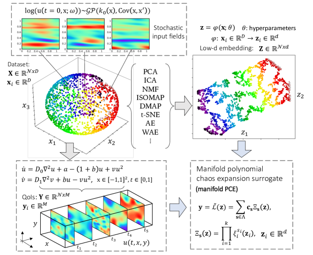
Figure 1: A schematic illustrating the m-PCE approach. The construction of a PCE surrogate whose inputs are projected on a lower-dimensional manifold, enables UQ in physics-based models associated with high-dimensional stochastic input fields.

3.1 Dimension reduction of high-dimensional inputs

The problem of dimensionality reduction is defined as follows. Given a high-dimensional dataset $\mathbf{X}=\{\mathbf{x}_{1},..,\mathbf{x}_{N}\}$ where $\mathbf{x}_{i}\in\mathbb{R}^{D}$, assume the intrinsic dimensionality of the dataset $d$ ($d\approx\mathcal{O}(10^{0-1})$), where $d<D$ and often $d\ll D$. The existence of an intrinsic dimensionality assumes that data points lie on or near a manifold of dimensionality $d$ that is embedded in the $D$-dimensional space. The structure of the $d$-dimensional manifold is unknown and it may even consist of a number of disconnected submanifolds [70]. The goal of DR is to identify a low-dimensional representation of the original dataset $\mathbf{Z}=\{\mathbf{z}_{1},..,\mathbf{z}_{N}\}$, $\mathbf{z}_{i}\in\mathbb{R}^{d}$, while retaining its meaningful properties. We denote this mapping as $\mathbf{z}=\phi(\mathbf{x};\theta)$, where $\phi:\mathbf{x}_{i}\in\mathbb{R}^{D}\rightarrow\mathbf{z}_{i}\in\mathbb{R}^{d}$ and $\theta\in\mathbb{R}^{n}$ represents the $n$-dimensional vector of parameters associated with the reduction method. The resulting dimension $d$ should ideally be close to the intrinsic dimension, however since this number is unknown a-priori, the problem is ill-posed and requires certain assumptions to be solved. The process of DR involves some transformation operation from the original to the reduced feature space [153]. Although certain methods allow an inverse transformation $\phi^{-1}:\mathbf{z}_{i}\in\mathbb{R}^{d}\rightarrow\mathbf{x}_{i}\in\mathbb{R}^{D}$ to map data back to the original space, for others this inverse mapping may not exist. Mathematically, to obtain the low-dimensional representation, an error measure $L(\mathbf{x};\theta)$ needs to be defined and minimized to estimate the optimal parameters $\hat{\theta}=\underset{\theta}{\arg\min}L(\mathbf{x};\theta)$. For example, when the inverse transformation $\phi^{-1}$ is available and the objective is data reduction without information loss, this function can be represented by the mean-squared reconstruction error [76].

Several methods studied in this work are considered convex, since the objective function does not contain local minima. The low-dimensional data representation is obtained by minimizing the convex objective function by means of an eigendecomposition. These include the PCA, kernel-PCA, ISOMAP, and DMAP. Sparse spectral techniques such as LLE and Laplacian eigenmaps focus on solving a sparse generalized eigenproblem which translates in retaining the local structure of the data. Non-convex techniques include multi-layer neural networks such as autoencoders. Blind source separation techniques such as ICA or NMF treat the high-dimensional dataset as a mixture of signals and aims to identify its individual sources.

The quality of the compressed data can be assessed by evaluating to what extent the local structure of the data is preserved. This evaluation can be performed by measuring the trustworthiness and the continuity of the low-dimensional embeddings. The reader is referred to [70] for more information.

3.2 Uncertainty propagation

Having defined a framework for identifying a low-dimensional representation of input random variables, we consider an unknown, closed form function $\mathcal{L}$, which allows us to map the reduced uncertain inputs to the QoIs as $\mathbf{y}=\mathcal{L}(\mathbf{z})=\mathcal{L}(\phi(\mathbf{x};\theta))$ where $\mathcal{L}:\mathbb{R}^{d}\rightarrow\mathbb{R}^{M}$. Let us assume that the $d$-dimensional reduced input random vector is formalized using an appropriate probability distribution $\mathbf{z}\sim p(\mathbf{z})$. The main goal of uncertainty propagation is to characterize the statistics of $\mathcal{L}(\mathbf{z})$. The first two moments, for example, are given by

$$\mu_{\mathcal{L}} =\int\mathcal{L}(\mathbf{z})p(\mathbf{z})d\mathbf{z}$$ (39a)

$$\sigma^{2}_{\mathcal{L}} =\int(\mathcal{L}(\mathbf{z})-\mu_{\mathcal{L}})^{2}p(\mathbf{z})d\mathbf{z},$$ (39b)

The above integrals can be approximated via standard Monte Carlo simulation. By the law of large numbers, the approximate mean $\hat{\mu}_{\mathcal{L}}$ and variance $\hat{\sigma}^{2}_{\mathcal{L}}$, converge to the true values as the samples size tends to infinity. For computationally demanding high-fidelity models, which is often the case in physics-based problems, a large number of evaluations is infeasible. We note, that these are essentially evaluations of the original model $\mathcal{M}$ as $\mathbf{y}=\mathcal{M}(\mathbf{x})=\mathcal{L}(\phi(\mathbf{x};\theta))$. Therefore, an approximate surrogate model $\widetilde{\mathcal{L}}$ is constructed using the set of reduced samples $\mathbf{z}$ and the corresponding model solutions $\mathbf{y}$ as training data. Once the surrogate model is appropriately trained it can be employed to inexpensively generate a very large number of approximate model evaluations in two steps: (1) the projection function $\phi:\mathbf{x}_{i}\in\mathbb{R}^{D}\rightarrow\mathbf{z}_{i}\in\mathbb{R}^{d}$ is used to encode new realizations of the high-dimensional inputs to a latent space and (2) the surrogate model $\widetilde{\mathcal{L}}:\mathbf{z}_{i}\in\mathbb{R}^{d}\rightarrow\mathbf{y}_{i}\in\mathbb{R}^{M}$ is used to map reduced data to the QoIs.

3.3 Surrogate modeling via polynomial chaos expansion

To construct a surrogate model $\widetilde{\mathcal{L}}$ that emulates the mapping $\mathbf{y}=\mathcal{L}(\mathbf{z})$ from the latent space to the output space i.e., $\mathcal{L}:\mathbb{R}^{d}\rightarrow\mathbb{R}^{M}$ we use non-intrusive PCE, an efficient and flexible surrogate modeling method. For the purposes of the method, the reduced input random variable $\mathbf{z}$, is considered to be defined on the probability space $\left(\Omega,\Sigma,P\right)$ and characterized by the joint probability density function (PDF) $\varrho_{\mathbf{Z}}:I\rightarrow\mathbb{R}_{\geq 0}$, where $I\subseteq\mathbb{R}^{d}$ is the image space, $\Omega$ the sample space, $\Sigma$ the set of events, and $P$ the probability measure.

In the following, we consider for simplicity a single model output, such that $Y\left(\omega\right)=\mathcal{L}\left(\mathbf{z}\left(\omega\right)\right)\in\mathbb{R}$, $\omega\in\Omega$. Under this assumption, the PCE is a spectral approximation of the form

$$\mathcal{L}(\mathbf{z})\approx\widetilde{\mathcal{L}}(\mathbf{z})=\sum_{s=1}^{S}c_{s}\Xi_{s}(\mathbf{z}),$$ (40)

where $c_{s}$ are scalar coefficients and $\Xi_{s}$ are multivariate polynomials that are orthonormal with respect to the joint PDF $\varrho_{\mathbf{Z}}$, such that

$$\mathbb{E}\left[\Xi_{s}\Xi_{t}\right]=\int_{S}\Xi_{s}\left(\mathbf{z}\right)\Xi_{t}\left(\mathbf{z}\right)\varrho_{\mathbf{z}}\left(\mathbf{z}\right)\mathrm{d}\mathbf{z}=\delta_{st},$$ (41)

where $\delta_{st}$ denotes the Kronecker delta. Depending on the PDF $\varrho_{\mathbf{z}}$, the orthonormal polynomials can be chosen according to the Wiener-Askey scheme [26] or be numerically constructed [154]. The joint PDF of independent random variables $z_{1},\dots,z_{k}$ and the multivariate orthogonal polynomials are given by

$$\varrho_{\mathbf{z}}\left(\mathbf{z}\right)=\prod_{i=1}^{d}\varrho_{z_{i}}\left(z_{i}\right),\hskip 10.0pt\Xi_{s}(\mathbf{z})\equiv\Xi_{\mathbf{s}}(\mathbf{z})=\prod_{i=1}^{d}\xi_{i}^{s_{i}}(z_{i}),$$ (42)

where $\varrho_{z_{i}}$ is the marginal PDF of random variable $z_{i}$ and $\xi_{i}^{s_{i}}$ are univariate polynomials of degree $s_{i}\in\mathbb{Z}_{\geq 0}$ and orthonormal with respect to the univariate PDF $\varrho_{z_{i}}$, such that

$$\mathbb{E}\left[\xi_{i}^{s_{i}}\xi_{i}^{t_{i}}\right]=\int_{z_{i}}\xi_{i}^{s_{i}}(z_{i})\xi_{i}^{t_{i}}(z_{i})\varrho_{z_{i}}(z_{i})\,\mathrm{d}z_{i}=\delta_{s_{i}t_{i}}.$$ (43)

The multi-index $\mathbf{s}=\left(s_{1},\dots,s_{k}\right)$ is equivalent to the multivariate polynomial degree and uniquely associated to the single index $s$ employed in Eq. (40), which can now be written in the equivalent form

$$\mathcal{L}(\mathbf{z})\approx\widetilde{\mathcal{L}}(\mathbf{z})=\sum_{\mathbf{s}\in\Lambda}c_{\mathbf{s}}\Xi_{\mathbf{s}}(\mathbf{z}),$$ (44)

where $\Lambda$ is a multi-index set with cardinality $\#\Lambda=S$. The choice of the multi-index set $\Lambda$ plays a central role in the construction of the PCE, as it defines which polynomials and corresponding coefficients form the PCE. The most common choice, as well as the one employed in this work, is that of a total-degree multi-index set, such that $\Lambda$ includes all multi-indices that satisfy $\left\|\mathbf{s}\right\|_{1}\leq s_{\max}$, $s_{\max}\in\mathbb{Z}_{\geq 0}$. In that case, the size of the PCE basis is $S=\frac{\left(s_{\max}+k\right)!}{s_{\max}!k!}$, i.e., it scales polynomially with the input dimension $k$ and the maximum degree $s_{\max}$.

Once the multi-index set $\Lambda$ is fixed, the only thing remaining to complete the PCE is to compute the coefficients, which is achieved here by means of regression [65, 59, 52, 69, 50]. In particular, the PCE coefficients are obtained by solving the penalized least squares problem

$$\underset{\mathbf{c}\in\mathbb{R}^{\#\Lambda}}{\arg\min}\left\{\frac{1}{N}\sum_{i=1}^{N}\left(\mathcal{L}(\mathbf{z}_{i})-\sum_{\mathbf{s}\in\Lambda}c_{\mathbf{s}}\Xi_{\mathbf{s}}\left(\mathbf{z}_{i}\right)\right)^{2}+\lambda J\left(\mathbf{c}\right)\right\},$$ (45)

where $\lambda\in\mathbb{R}$ is a penalty factor, $J\left(\mathbf{c}\right)$ is a penalty function acting on the vector of PCE coefficients $\mathbf{c}\in\mathbb{R}^{\#\Lambda}$, and $\mathbf{Z}=\left\{\mathbf{z}_{i}\right\}_{i=1}^{N}$ is an experimental design (ED) of random variable realizations with corresponding model outputs $\mathbf{Y}=\left\{\mathbf{y}_{i}\right\}_{i=1}^{N}$. Common choices for the penalty function $J(\mathbf{c})$ are the $\ell_{1}$ and $\ell_{2}$ norms, in which cases problem (45) is referred to as LASSO (least absolute shrinkage and selection operator) and ridge regression, respectively. Removing the penalty term results in an ordinary least squares (OLS) regression problem.

3.3.1 PCE on latent spaces

The theoretical challenges in applying the PCE to the reduced dimensional vector $\mathbf{z}$ are that its probability measure is not generally known exactly, it may take a non-standard form, and it may include dependencies between variables. Several techniques have been developed to address these challenges. For non-standard measures, orthogonal polynomials can be constructed by Stiltjes or Gram-Schmidt orthogonalization [154, 155]. Furthermore, for non-standard or unknown measures the polynomials can be constructed to be orthogonal with respect to statistical moments rather than the joint pdf, using an approached termed arbitrary PCE (aPCE) [28]. Finally, dependencies can either be ignored altogether or they can be explicitly modeled through copulas and a corresponding Rosenblatt transformation to obtain independent uniform random variables [156].

However, for practical purposes the reduced input variables can be approximated as either uniformly or normally distributed and independent. Although this violates certain theoretical considerations, it does not lead to significant differences in the model accuracy as illustrated in the examples below. Furthermore, it has been shown in the literature that ignoring the input dependencies results in good surrogate model performance, since complex nonlinear input transformations, e.g., via the Rosenblatt transform, are avoided [157, 156, 76]. Herein, we approximate the reduced input variables as independent and uniformly distributed over the support of the reduced data set. Again, we emphasize that this is done for simplicity and because it is demonstrated to give sufficiently accurate results. If these assumptions become problematic, either due to theoretical reasons or due to a lack of predictive accuracy, one can always resort to the methods discussed above to improve the PCE approximation. There are no constraints against using these methods within the m-PCE framework.

Furthermore, in the proposed framework QoIs are vector-valued, usually representing fields that evolve in space and time, and the PCE approximation described in the previous Section is applied element-wise. The way the surrogate is formulated is that a basis is constructed, and the coefficients are computed for each output element (location in the field). The correlation between output grids is implicitly taken into account, as the learned sets of PCE coefficients are highly correlated. The m-PCE approach can be extended to perform dimension reduction in both input and output fields which results in the construction of very few PCE surrogates for output components that do not have the same spatial dependence [42].

3.3.2 Error estimation of surrogate predictions

To assess the predictive accuracy of the PCE surrogate, we employ two metrics. The first scalar metric is the relative $L_{2}$ error given by

$$L_{2}(\mathbf{y}_{\text{pred}},\mathbf{y}_{\text{ref}})=\frac{\|\mathbf{y}_{\text{pred}}-{\mathbf{y}_{\text{ref}}\|}_{2}}{{\|\mathbf{y}_{\text{ref}}\|}_{2}},$$ (46)

where ${\|\cdot\|}_{2}$ denotes the standard Euclidean norm and $\mathbf{y}_{\text{pred}},\mathbf{y}_{\text{ref}}$ are the prediction and reference responses respectively. As a second scalar metric we introduce is the $R^{2}$ score, also known as the coefficient of determination, defined as

$$R^{2}=1-\frac{{\sum}_{i=1}^{w}\Big{(}\mathbf{y}_{\text{pred},i}-\mathbf{y}_{\text{ref},i}\Big{)}^{2}}{{\sum}_{i=1}^{w}\Big{(}\mathbf{y}_{\text{ref},i}-\overline{\mathbf{y}}_{\text{ref}}\Big{)}^{2}},$$ (47)

where $w$ is the total number of mesh points of the QoI and $\overline{\mathbf{y}}_{\text{ref}}$ is the mean reference response. The above metrics are computed for a holdout test dataset of transformed inputs and model outputs $\{{\mathbf{z}^{*}_{i}\in\mathbb{R}^{d}},\mathbf{y}^{*}_{i}\in{\mathbb{R}^{M}}\}_{i=1}^{N^{*}}$ where $N^{*}$ is the total number of test realizations.

3.4 Hyperparameter optimization

Hyperparameter optimization refers to the problem of optimizing a loss function over a graph-structured configuration space [158]. The mapping of high-dimensional inputs to a latent space, $\mathbf{z}=\phi(\mathbf{x};\theta)$ is associated with $n$ hyperparameters. The domain of the $\hat{n}$-th hyperparameter is denoted as $\Theta_{\hat{n}}$ and the overall configuration space as $\boldsymbol{\Theta}=\Theta_{1}\times\Theta_{2}\times\cdots\times\Theta_{n}$ thus the vector of hyperparameters is denoted as $\theta\in\boldsymbol{\Theta}$. In a more naive approach one resorts to extensive experimentation or grid search to obtain a suitable model which can be extremely time-consuming as it suffers from the curse of dimensionality. Hyperparameter optimization algorithms optimize variables which can be real (e.g., learning rate) or integer-valued (e.g., number of layers in an ANN), typically with bounded domains, binary (e.g., early stopping or not), or categorical (e.g., choice of the optimizer) [159]. Given an infinite-sample dataset $\mathcal{D}$, the objective reads

$$\theta^{*}=\underset{\theta\in\boldsymbol{\Theta}}{\arg\min}\mathbb{E}_{(\mathbf{X},\mathbf{X}_{*})\sim\mathcal{D}}\mathbf{V}(\Lambda,\phi_{\theta},\mathbf{X},\mathbf{X}_{*}),$$ (48)

where $\mathbf{V}(\Lambda,\phi_{\theta},\mathbf{X},\mathbf{X}_{*})$ is the validation protocol which measures the loss $\Lambda$ of the model $\phi_{\theta}$ with hyperparameters $\theta$ when trained on the dataset $\mathbf{X}$ and tested on dataset $\mathbf{X}_{*}$. In practice, we have a finite set of samples thus we compute the approximate expectation. Popular choices of the validation protocol $\mathbf{V}(\cdot)$ include the holdout and cross-validation (CV) error [159, 160].

In this work, we found that certain DR methods are competitive with default parameters and do not benefit much from parameter tuning. These are typically simpler methods like kernel-PCA or DMAP which tend to have a small number of hyperparameters. However, for more complex models (e.g., ANNs) parameter tuning has the potential to boost the model performance compared to using default parameters. In this work, hyperparameter values are chosen based on the predictive ability of the surrogate model and not solely on the performance of the DR method (e.g., to what extent the local structure is preserved or how small the error is between original samples and inverse-mapped samples). We use default parameters for methods which do not benefit much from parameter tuning and we manually select after experimentation hyperparameter values for more complex DR methods such as AE or WAE. Therefore, we do not expect that implementing expensive optimization would significantly alter the comparison results or the drawn conclusions. Nevertheless, optimization can be straightforwardly integrated into the proposed framework for a more systematic experimentation and model selection.

4 Numerical examples

We compare the performance of the thirteen manifold learning methods for high-dimensional UQ on the following three applications: (i) the 1D stochastic Poisson’s equation, (ii) a stochastic elliptic PDE modeling a 2D diffusion process, and (iii) a 2D stochastic time-dependent PDE describing an autocatalytic reaction. For each application, we compare the performance of each method and provide numerical evidence in terms of generalization error and computational cost which consists of the CPU time for both the DR and surrogate modeling tasks. All analyses in this paper were carried out on a 2.8 GHz Quad-Core Intel Core i7 X CPU.

4.1 1D stochastic Poisson’s equation

Consider the following one-dimensional stochastic Poisson’s equation with homogeneous boundary conditions

$$\begin{split}-\odv[2]{}{x}u&=f(x;\omega),\ \ x\in[-1,1]\ \text{and}\ \omega\in\Omega,\\ u(-1)&=u(1)=0\end{split}$$ (49)

where $\Omega$ is the random space and the forcing term is given by the following Gaussian random process

$$f(x;\omega)\sim\mathcal{GP}(f_{0}(x),\text{Cov}(x,x^{\prime}))$$ (50)

with mean function and covariance function

$$\begin{split}f_{0}(x)&=0.1\sin(\pi x)\\ \text{Cov}(x,x^{\prime})&=\sigma^{2}\exp\bigg{(}-\frac{(x-x^{\prime})^{2}}{l_{c}^{2}}\bigg{)},\end{split}$$ (51)

where $\sigma=\sqrt{20}$ is the standard deviation and $l_{c}=0.2$ the correlation length.

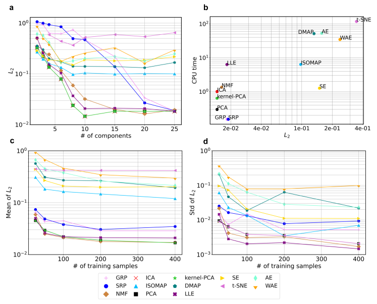
Figure 2: Comparison of the accuracy of the thirteen DR methods as a function of (a) the number of reduced components and (b) the CPU time of the trained PCE surrogate evaluated on the testing set of $N^{*}=1000$ data. Furthermore, the mean (c) and standard deviation (d) of the relative $L_{2}$ error are shown for $d=20$ as a function of the number of training samples based on repeated runs with different datasets.

The proposed approach is employed to learn the mapping from $f(x;\omega)$ to the solution $u(x;\omega)$. We discretize the 1D domain $[-1,1]$ into $t=1024$ points and generate $N=1000$ realizations of the Gaussian stochastic process, $\{f_{i}=f(x;\omega)\}_{i=1}^{N}$ using the Karhunen Loéve expansion (KLE) as

$$f(x)=f_{0}(x)+\sum_{i=1}^{N_{t}}\sqrt{\lambda_{i}}\theta_{i}f_{i}(x),$$ (52)

where $\lambda_{i}$ and $f_{i}(x)$ are the eigenvalues and eigenvectors respectively of the covariance function $\text{Cov}(x,x^{\prime})$ determined by solving the homogeneous Fredholm integral eigenvalue problem and $\theta_{i}$ are iid $N(0,1)$ random variables [103]. In the KLE, we retain $N_{t}=1024$ (the full rank of the expansion) which is intentionally set to a conservatively large number to allow us to identify the intrinsic dimension through DR. Next, we translate the Gaussian stochastic process generated in Eq. (52) to a non-Gaussian stochastic process [161] as follows

$$f^{\text{NG}}(x)=f_{0}(x)+F_{\text{NG}}^{-1}\Bigg{(}\Phi\Bigg{(}\frac{\sum_{i=1}^{N_{t}}\sqrt{\lambda_{i}}\theta_{i}f_{i}(x)}{\sigma}\Bigg{)}\Bigg{)}$$ (53)

where $F_{\text{NG}}^{-1}(\cdot)$ represents the inverse cumulative distribution function of the non-Gaussian distribution and $\Phi$ represents the cdf of the standard normal distribution. In this example, we chose the non-Gaussian distribution to be the uniform distribution $U[a,b]$, where $a=-15$ and $b=15$. The transformed non-Gaussian stochastic process is therefore given by

$$f^{\text{NG}}(x)=f_{0}(x)+a+(b-a)*\Phi\Bigg{(}\frac{\sum_{i=1}^{N_{t}}\sqrt{\lambda_{i}}\theta_{i}f_{i}(x)}{\sigma}\Bigg{)}$$ (54)

$$f^{\text{NG}}(x)=f_{0}(x)+a+(b-a)*\Bigg{(}1+\frac{1}{2}\mathrm{erf}\Bigg{(}\frac{\sum_{i=1}^{N_{t}}\sqrt{\lambda_{i}}\theta_{i}f_{i}(x)}{\sqrt{2}\sigma}\Bigg{)}\Bigg{)}$$

where $\mathrm{erf}(z)=\frac{2}{\sqrt{\pi}}\int_{0}^{z}\exp\left(-t^{2}\right)\mathrm{d}t$ is the error function.

We solve the equation with the finite difference (FD) method and generate the corresponding model responses $\{u_{i}=u(x;\omega)\}_{i=1}^{N}$. Therefore we construct the training dataset of inputs $\mathbf{X}=\{\mathbf{x}_{1},..,\mathbf{x}_{N}\}$ where $\mathbf{x}_{i}\in\mathbb{R}^{1024}$ and outputs $\mathbf{Y}=\{\mathbf{y}_{1},..,\mathbf{y}_{N}\}$ where $\mathbf{y}_{i}\in\mathbb{R}^{1024}$. To evaluate the performance of the trained model, we generate another $N^{*}=1000$ samples of $f(x;\omega)$ and corresponding trajectories $u(x;\omega)$ independently of the training data. We denote this dataset as $\mathbf{X}^{*}=\{\mathbf{x}_{1},..,\mathbf{x}_{N^{*}}\}$, $\mathbf{Y}^{*}=\{\mathbf{y}_{1},..,\mathbf{y}_{N^{*}}\}$ of inputs and model outputs respectively. The quality of the surrogate predictions are evaluated based on the metrics presented in Section 3.3.2.

We compare the performance of the trained PCE surrogate for all DR methods in Figure 2. Figures 2(a) and 2(b) show the relative $L_{2}$ error and CPU training time of the trained m-PCE where each color/symbol corresponds to one of the thirteen DR methods. We observe that the simple DR methods converge fast and with high accuracy. The optimal response in terms of relative error is observed by the PCA, k-PCA, ICA methods which resulted in similar relative errors. We note, that in this example a linear kernel has been chosen for k-PCA therefore the method essentially results in standard PCA. However, the CPU time between these methods varies significantly as shown in Figure 2(c). Taking into account both the prediction accuracy and CPU time, PCA PCE performed optimally resulting in a relative error of $L_{2}=2.80\cdot 10^{-5}$ where the PCE surrogate is constructed with $d=20$ approximately independent input random variables. Furthermore, in 2(c),(d) we plot the mean and standard deviation of the relative $L_{2}$ error versus the number of training data. We observe that the best performing methods converge rapidly (with only $\sim 100$ training points) to an accurate solution with small uncertainty, while more expensive methods such as AE and WAE result in a much higher mean value and error.

In Figure 3, the predictive accuracy of the optimal PCA PCE surrogate is illustrated. Three random realizations of the input stochastic process are generated and the surrogate response is compared with the ground truth solution computed with the FD solver. The comparison, results in scalar error measures in the order of $10^{-5}$, revealing the powerful predictive ability of the surrogate. Finally, in Figure 4, the mean response and the associated $95\%$ CI are computed for all $N^{*}$ test data. We observe that the m-PCE has the ability to perform moment estimation with very high accuracy.

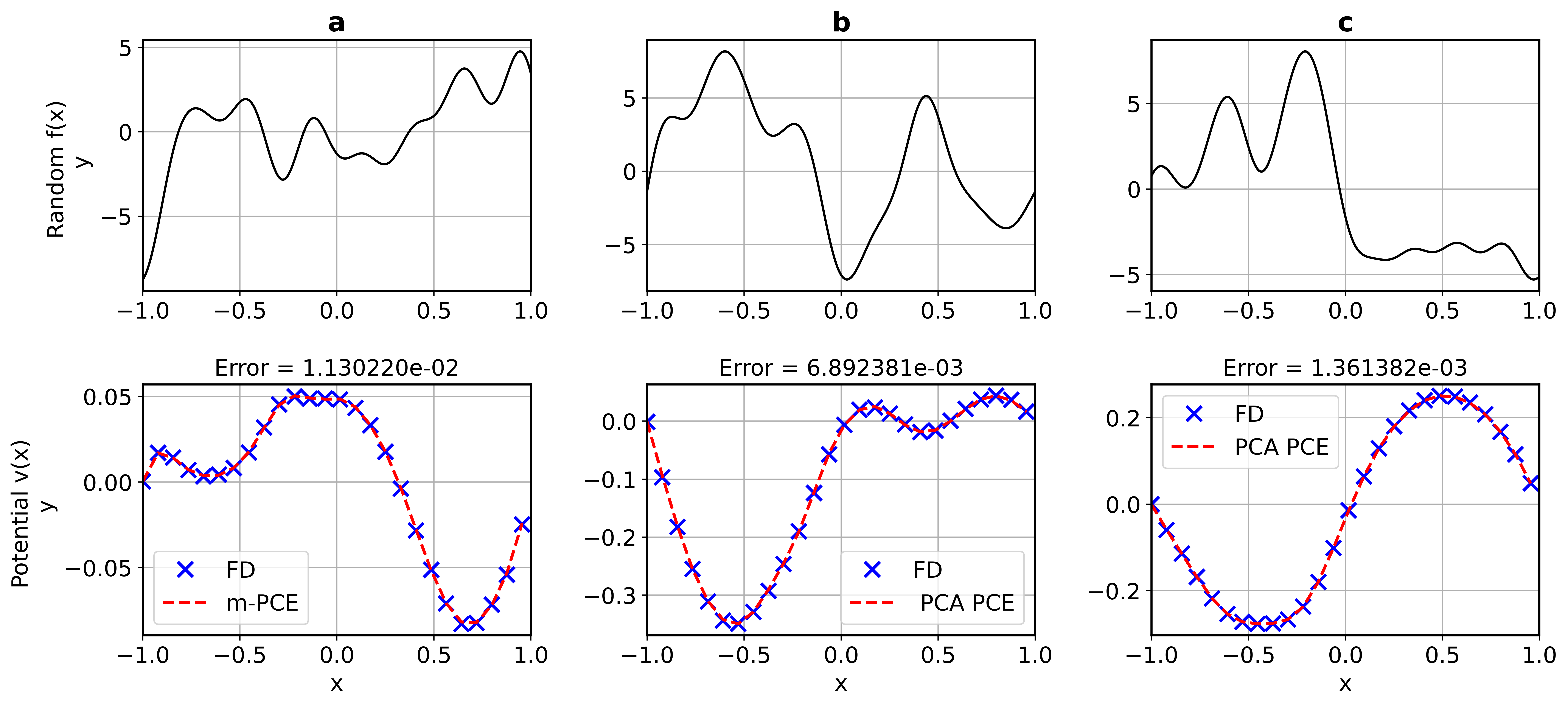
Figure 3: PCA PCE prediction for three random realizations of the inputs stochastic process. Blue ‘x’s represent the solution with the numerical solver (finite differences or FD) and red dashed curves the m-PCE response.

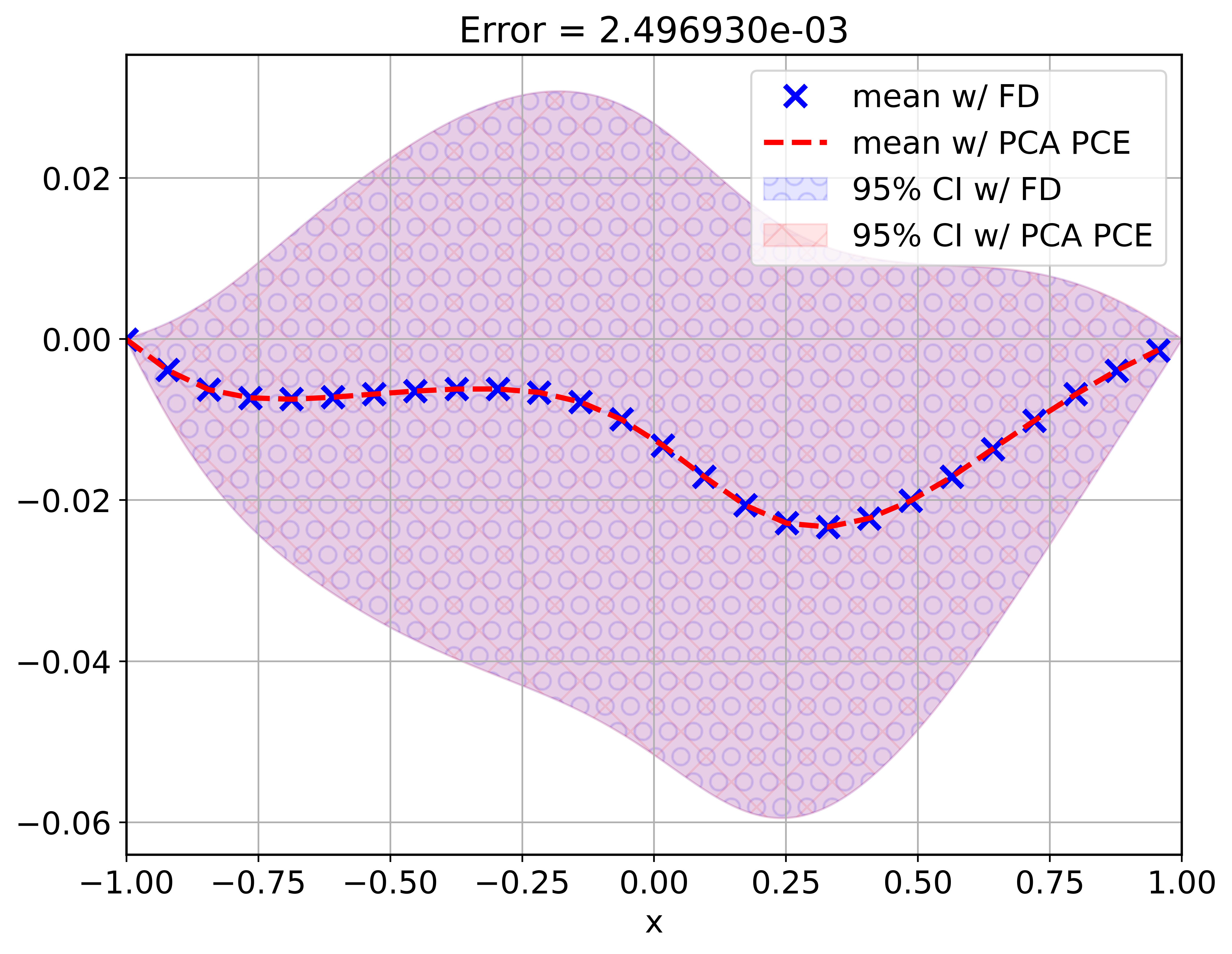
Figure 4: Estimation of the mean and $95\%$ CI of solution with FD and m-PCE.

4.2 2D stochastic steady-state heat equation

Consider the following elliptic PDE on the 2-d unit square domain which describes steady-state diffusion processes

$$\nabla(D(\mathsf{x})\nabla u(\mathsf{x})) =0,\ \forall\mathsf{x}\in[0,1]^{2}$$ (55a)

$$\text{BC:}\hskip 5.0ptu =0,\hskip 2.0pt\forall x=1,$$ (55b)

$$u =1,\hskip 2.0pt\forall x=0,$$ (55c)

$$\frac{\partial u}{\partial n} =0,\hskip 2.0pt\forall y=0\hskip 2.0pt\text{and}\hskip 2.0pty=1,$$ (55d)

where $\mathsf{x}=(x,y)$ represents the spatial coordinates in 2-d Euclidean space. In this example, randomness comes from the spatially varying diffusion coefficient $D(\mathsf{x})$, which is modeled and sampled from a log-normal random field such that

$$\log D(\mathsf{x})\sim\mathcal{GP}(D(\mathsf{x})|\mu(\mathsf{x}),\text{Cov}(\mathsf{x},\mathsf{x}^{\prime})),$$ (56)

where $\mu(\mathsf{x})$ and $\text{Cov}(\mathsf{x},\mathsf{x}^{\prime})$ are the mean and covariance functions respectively. For simplicity, we set $\mu(\mathsf{x})=0$, while the covariance matrix is given by the squared exponential kernel as

$$\text{Cov}(\mathsf{x},\mathsf{x}^{\prime})=\text{exp}\Bigg{(}-\frac{|x-x^{\prime}|}{\ell_{x}}-\frac{|y-y^{\prime}|}{\ell_{y}}\Bigg{)},$$ (57)

where $\ell_{x}$, $\ell_{y}$ are the correlation lengthscales along the $x$ and $y$ spatial directions, respectively. To generate realizations of the input stochastic diffusion field we again employ the KLE with a full rank of 784 random variables, again to allow the DR to identify the intrinsic dimension. Traditionally, one would construct a surrogate model to map the input stochastic fields $D(\mathsf{x})$ to the model output $u(\mathsf{x})$ for constant values of the lengthscale parameters. Similarly to [88], we aim to remove the restrictions of the lengthscales and therefore we construct a surrogate which is trained to predict the numerical solution $u(\mathsf{x})$ for novel realizations of the discretized random input fields for arbitrary lengthscale values.

Figure 5: Randomly generated lengthscale pairs with LHS for the training dataset (blue) and uniform lengthscale pairs (red) for the validation dataset.

The simulation takes place in a square domain $\Omega=[0,1]\times[0,1]$, discretized into $32\times 32=1024$ volume cells and the PDE is solved with the finite volume method (FVM). To construct the training dataset, we first obtain the design of lengthscale pairs $\mathbf{L}=(\ell_{x},\ell_{y})$. We generate $n=60$ lengthscale pairs using the sampling algorithm proposed in [88] to bias samples toward lower length-scales and for each pair, $N=70$ realizations of the input stochastic field. For these $n\cdot N=4200$ total realizations we solve the forward model and split the dataset into $N=2000$ training and $N^{*}=2200$ test data. We denote the input train data with $\mathbf{X}=\{\mathbf{x}_{1},..,\mathbf{x}_{N}\}$ where $\mathbf{x}_{i}\in\mathbb{R}^{1024}$ and the output solutions with $\mathbf{Y}=\{\mathbf{y}_{1},..,\mathbf{y}_{N}\}$ where $\mathbf{y}_{i}\in\mathbb{R}^{1024}$. In Figure 5, the lengthscale pairs are shown. We also generate input fields and model solutions for a set of $\hat{n}=100$ lengthscale pairs uniformly distributed in the square spatial domain as an out-of-distribution (OOD) validation set to test generalizability, also shown in Figure 5, with $\hat{N}=50$ samples for each pair. The generalization ability of the trained surrogate will be tested for this OOD validation dataset $(\hat{\mathbf{X}},\hat{\mathbf{Y})}$ which is not used during the training of the model.

4.2.1 Prediction for arbitrary lengthscales

Figure 6: Comparison of the accuracy of the thirteen DR methods as a function of the (a) number of reduced components and (b) the CPU time of the trained PCE surrogate evaluated on the dataset $(\hat{\mathbf{X}},\hat{\mathbf{Y})}$. Furthermore, the mean (c) and standard deviation (d) of the relative $L_{2}$ error are shown for $d=15$ as a function of the number of training samples based on repeated runs with different datasets.

Figure 7: AE PCE prediction for three random realizations of the input diffusion field $D(\mathsf{x})$.

Figure 8: Average of the (left column) relative $L_{2}$ errors and (right column) $R^{2}$ scores for each uniform lengthscale pair. ‘x’ markers represent the training lengthscale pairs generated with LHS and solid ‘o’ markers the uniform lengthscale pairs used for validating the (a) AE PCE and (b) PCA PCE surrogate.

A simple PCA on the $1024$-dimensional input data reveals that $15$ dimensions account for $\approx 87\%$ of the variance of the data. We compare the performance of the trained PCE surrogate in Figure 6 evaluated on the validation dataset of uniformly distributed lengthscales $(\hat{\mathbf{X}},\hat{\mathbf{Y})}$. Figures 6(a) shows the relative $L_{2}$ error of the trained m-PCE as a function of the reduced space dimension (number of components) where each color corresponds to one of the thirteen DR methods. We observe that the WAE, AE and LLE performed best in terms of predictive accuracy, while GRP and SRP resulted in the largest error. The optimal response in terms of relative error is observed by the AE PCE and in terms of CPU time by the PCA PCE, where the surrogate is constructed with a diffusion input field modeled as a nonlinear combination of $d=15$ and $d=10$ independent standard normal random variables respectively and a maximum polynomial degree of $s_{max}=2$ for both cases. The resulting average relative error is measured as $L_{2}=3.30\cdot 10^{-2}$ and $L_{2}=3.95\cdot 10^{-2}$ respectively. Figure 6(b), shows the CPU time versus the relative $L_{2}$ error. Although AE, WAE and LLE performed best, their computational cost is significantly higher (two orders of magnitude). ICA, PCA and NMF methods provide a much faster alternative while still exhibiting a small validation error $L_{2}\approx 4\cdot 10^{-2}$. Finally, in Figure 6(c),(d) the surrogate is trained for different training datasets to obtain confidence intervals for the predictions. The mean and standard deviation are shown as a function of the number of training samples. We observe that the accuracy for all methods converges quickly (within $\approx 200$ training samples) with small uncertainty, thus small datasets suffice.

In Figure 7, the results of the optimal surrogate in terms of predictive accuracy (i.e., AE PCE) are shown for three random test realizations of the input diffusion field $D(\mathsf{x})$. These three fields, demonstrate the lengthscale variability which renders the input dataset challenging for the construction of the surrogate model. As expected, the error increases for finer lengthscales in both spatial dimensions which results in input fields with more variation and thus more intricate underlying structure. The average of the relative $L_{2}$ errors and the $R^{2}$ scores for each uniform lengthscale pair is calculated for both the AE PCE (highest accuracy) and PCA PCE (highest speed) and shown in Figure 8. We observe that the surrogate performs very well even for input fields with lengthscale pairs that have not been included in the training of the model. Based on these results, we suggest that one should sample more pairs that corresponds to small $\ell_{x}$ values since in this zone we compute the highest relative errors. Comparing these plots with the equivalent ones from a similar approach based on the training of DNNs for both the DR and surrogate modeling tasks, known as the ‘Deep UQ’ proposed in [88], we observe that the proposed AE PCE approach results in comparable response in terms of predictive accuracy and generalization, with less training data and CPU time. Therefore, the m-PCE can provide a cost-effective approach for constructing surrogates with less trainable parameters, when small data is available with limited computational resources.

4.2.2 Uncertainty propagation

Figure 9: Mean and variance field of PDE solution $u(\mathsf{x})$ for $\ell_{x}=0.15$ and $\ell_{y}=0.25$. The fields are computed with MCS (first column) and (a) AE PCE and (b) PCA PCE (second column) for $10^{4}$ samples. Third column shows the relative error as a field and also the scalar relative $L_{2}$ error (average) and $R^{2}$ score.

The trained m-PCE surrogate has been generalized for arbitrary lengthscales and will be now used for uncertainty propagation with fixed lengthscale values $\ell_{x}=0.15$ and $\ell_{y}=0.25$. We generate a large number of input samples i.e., $10^{4}$ and compute with both MC simulation and the proposed surrogate the mean and variance fields of the solution $u(\mathsf{x})$. In addition we compute the probability density of the QoI at two fixed points in space: $\mathsf{x}_{1}=(0.323,0.645)$ and $\mathsf{x}_{2}=(0.806,0.258)$.

We compare the mean and variance fields computed with MCS and m-PCE in Figure 9. The relative error between the fields as well as the average relative $L_{2}$ error and $R^{2}$ score are computed. All error measures show a very good match between the reference and predicted mean fields. The variance fields have higher relative error, partially attributed to their small magnitude, which appears in the denominator of the $L_{2}$ error metric. However, the scalar error measures remain fairly low. We note that smaller lengthscales $\ell_{x},\ell_{y}$ will likely result in higher errors, however generating more training samples for lengthscale pairs in these regions will enhance the performance and accuracy of the surrogate. Finally, Figure 10 shows the comparison between the probability density of the solution $u(\mathsf{x})$ for two spatial points computed with MCS and both AE PCE and PCA PCE. We observe that even if some accuracy is sacrificed over cost, m-PCE is able to capture the density of the solution to a satisfactory degree.

Figure 10: Density of PDE solution $u(\mathsf{x})$ for $\mathsf{x}_{1}=(0.323,0.645)$ and $\mathsf{x}_{2}=(0.806,0.258)$ with MCS (blue) and (a) AE PCE and (b) PCA PCE (red).

4.3 2D time-dependent stochastic Brusselator model

Finally, consider the stochastic Brusselator model, describing the dynamics for a type of an autocatalytic oscillating chemical reaction [162]. The Brusselator model is characterized by the following reactions

$$A \xrightarrow{k_{1}}X\quad$$ (58a)

$$B+X \xrightarrow{k_{2}}Y+D$$ (58b)

$$2X+Y \xrightarrow{k_{3}}3X$$ (58c)

$$X \xrightarrow{k_{4}}E$$ (58d)

where a reactant A is converted to a final product $E$, through four steps and four additional species, $X,B,Y$ and $D$. In Eq. (58)(b and c), bimolecular and autocatalytic trimolecular reactions are shown respectively. Based on this reaction, species $E$ is resulted from species $X$ which in turn results from Eq. (58)(a and c). We consider that A and B are in vast excess and thus can be modeled at constant concentration. Through the law of mass action the Brusselator system can be described by the following model

$$\begin{split}\frac{\partial u}{\partial t}&=D_{0}\nabla^{2}u+a-(1+b)u+vu^{2}\\ \frac{\partial v}{\partial t}&=D_{1}\nabla^{2}v+bu-vu^{2},\hskip 10.0pt\mathsf{x}\in[0,1]^{2},\ t\in[0,1],\end{split}$$ (59)

where $\mathsf{x}=(x,y)$ are the spatial coordinates, $D_{0},D_{1}$ represent the diffusion coefficients, $a=\{A\},b=\{B\}$ are constant concentrations and $u=\{X\},v=\{Y\}$ represent the concentrations of reactant species $X,Y$. Depending on the values of the parameters the Brusselator model can exhibit a limit cycle, a Hopf bifurcation and also a chaotic behaviour [162]. We choose $a=1$, $b=3$, $D_{0}=1$ and $D_{1}=0.1$ for which the system is in an unstable regime approaching a limit cycle which forces the system to oscillate after sufficient time.

Figure 11: Comparison of surrogate response for thirteen DR methods for input random fields of increasing complexity. Subplots a,b,c, represent realizations of Gaussian random fields of $v(t=0,x,y)$ with the SRM method for $(\alpha_{1}^{(1)},\alpha_{2}^{(1)})=(3\cdot 10^{3},25),(\alpha_{1}^{(2)},\alpha_{2}^{(2)})=(750,14)$ and $(\alpha_{1}^{(3)},\alpha_{2}^{(3)})=(50,10)$ respectively and the plots below show the respective errors. Red and blue dashed lines represent the optimal relative error and $R^{2}$ score respectively from all three cases to serve as a reference value and are shown in all subplots (d-i).

Figure 12: (a) CPU time versus relative error for input random realizations generated with SRM with $(\alpha_{1}^{(1)},\alpha_{2}^{(1)})=(3\times 10^{3},25)$. (b),(c) present the mean and standard deviation of relative $L_{2}$ error respectively for $d=20$ retained components as a function of the number of training samples.

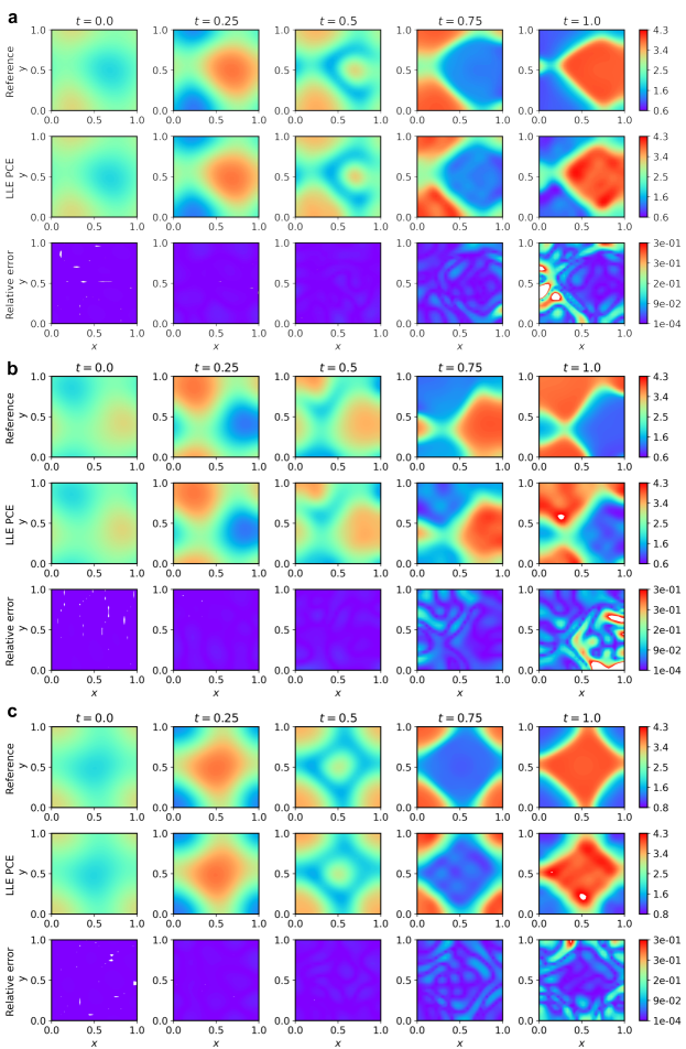
Figure 13: Comparison of the time evolution of $v(t,x,y)$ between reference and LLE PCE response for three input realizations generated with SRM with $(\alpha_{1}^{(1)},\alpha_{2}^{(1)})=(3\times 10^{3},25)$. The reference solution and the relative error are shown for three test cases (a),(b),(c), and five time steps, i.e., $t=(0,0.25,0.5,0.75,1)$.

The simulation takes place in a square domain $\Omega=[0,1]\times[0,1]$, discretized with $28\times 28=784$ mesh points. The proposed approach is employed to learn the mapping from $v(t=0,x,y)$ to the solution $v(t,x,y)$. To construct the training dataset, we generate realizations of the input Gaussian stochastic field which represents the spatially varying initial conditions of quantity $v$. We employ the spectral representation method (SRM) [163] which expands the stochastic process as a Fourier-type expansion of cosines as

$$A(x,y)=\sqrt{2}\sum_{i=1}^{M}\sum_{j=1}^{M}\{\sqrt{2S(\kappa_{1i},\kappa_{2j})\Delta\kappa_{1}\Delta\kappa_{2}}\cos{(\kappa_{1i}x+\kappa_{2j}y+\phi^{(1)}_{ij})}+$$ (60)

$$+\sqrt{2S(\kappa_{1i},-\kappa_{2j})\Delta\kappa_{1}\Delta\kappa_{2}}\cos{(\kappa_{1i}x-\kappa_{2j}y+\phi^{(2)}_{ij})}\},$$

where $S(\kappa_{1},\kappa_{2})$ is the discretized power spectrum, taking the following form

$$S(\kappa_{1},\kappa_{2})=\alpha_{2}(\kappa_{1}^{2}+\kappa_{2}^{2})e^{-\alpha_{1}\sqrt{\kappa_{1}^{2}+\kappa_{2}^{2}}}$$ (61)

$\Delta\kappa_{1}=\Delta\kappa_{2}=0.01$ is the wavenumber discretization, $\kappa_{1u}=\kappa_{2u}=1.28\text{rad}/\text{sec}$ the upper cutoff wavenumber which yields $M=128$, and thus a total of 32,768 random phase angles $\phi_{ij}$ that are uniformly distributed in $[0,2\pi]$. The two parameters of the discretized spectrum $(\alpha_{1},\alpha_{2})$ dictate the complexity and thus the intrinsic dimensionality of the generated random fields. We are considering the following three cases: $(\alpha_{1}^{(1)},\alpha_{2}^{(1)})=(3\cdot 10^{3},25),(\alpha_{1}^{(2)},\alpha_{2}^{(2)})=(750,14)$ and $(\alpha_{1}^{(3)},\alpha_{2}^{(3)})=(50,10)$. Using SRM in UQpy [99], we generate a dataset of $N=800$ input random fields $\mathbf{X}=\{\mathbf{x}_{1},..,\mathbf{x}_{N}\}$ where $\mathbf{x}_{i}\in\mathbb{R}^{784}$ for each one of the three cases. The initial condition of $u$ is represented by a constant field with a value $u(t=0,x,y)=a$. By solving the PDE system in the time interval $t=[0,1]$ for $\delta t=10^{-2}$, we measure the spatial behaviour of $v(\mathsf{x})$ at ten different time points, for the $N$ input stochastic field realizations. We solve the system with finite differences and vectorize solutions thus obtaining the output response matrices as $\mathbf{Y}=\{\mathbf{y}_{1},..,\mathbf{y}_{N}\}$ where $\mathbf{y}_{i}\in\mathbb{R}^{7840}$. We collect another $N^{*}=1000$ input samples and corresponding model outputs to evaluate the performance of the surrogate model.

We note that constructing a surrogate model for input random fields generated with the SRM method may be more challenging than for fields generate using the KLE because the SRM provides a much less compact representation of the stochastic process and therefore the intrinsic dimensionality of the fields may be significantly higher. The computational complexity of the PCE surrogate training increases exponentially with the dimensionality of inputs, therefore the goal is to keep this number as small as possible. Furthermore, in this application we aim to predict the full time evolving solution of the Brusselator model and not a single solution snapshot, which introduces an additional challenge to the construction of an accurate surrogate.

In Figure 11, we compare the predictive accuracy of the m-PCE surrogate for input random fields generated with the SRM method for the three cases discussed above. Each column shows a representative input random field, the relative error and $R^{2}$ score for all thirteen DR methods as a function of the embedding dimensionality (number of components). Figure 12 (a), shows the $L_{2}$ error vs. CPU time for each of the 13 methods for the case of $(\alpha_{1}^{(1)},\alpha_{2}^{(1)})=(3\times 10^{3},25)$. These results show that LLE performs best when considering random fields with large lengthscale value (higher decay parameter $\alpha_{2}$) resulting in an average relative error of $L_{2}=2.97\cdot 10^{-2}$. However, k-PCA seems to perform better when considering the CPU time, and having only slightly higher $L_{2}$ error. Figure 12 (b),(c) show the mean and standard deviation of relative $L_{2}$ error for all 13 methods for $d=20$. We observe a fast convergence of the error with respect to the number of training samples with small uncertainty for most methods. However, certain methods such as LLE, AE and WAE require more data to reach convergence. Furthermore, from Figure 11, PCA, k-PCA and ICA seem to outperform LLE in terms of predictive accuracy of the surrogate when the lengthscale of random fields is smaller and thus the complexity is higher. The accuracy of the PCE surrogate fluctuates significantly when the t-SNE method is employed, which is most likely attributed to convergence issues related to non-convex optimization. Interestingly, the surrogate accuracy for certain DR methods, reaches a minimum point and subsequently increases. One possible explanation is that the DR method has identified the intrinsic dimensionality of input data, therefore adding more components results in including redundant and noisy features. Another explanation, is that even if only important features are preserved, the resulting reduced space is not suitable for the construction of an accurate mapping - perhaps DR results in non-continuous disjoint reduced input subspaces which could be remedied with the construction of multiple local PCE surrogate models.

Finally, in Figure 13 we present the evolution of $v(t,x,y)$ for 5 time steps $t=(0,0.25,0.5,0.75,1)$. The reference response is shown in the first row, the LLE PCE (optimal surrogate for $(\alpha_{1}^{(1)},\alpha_{2}^{(1)})$) in the second row, and the point-wise relative error in the third row, for each one of the three test cases (a,b,c). We observe that early in the simulation, the relative error is on the order of $10^{-4}$, while for the last time step the error is higher, although still within acceptable bounds. We note that the current application allowed us to identify certain limitations of the proposed approach. Particularly, the m-PCE accuracy diminishes when input random fields have high local variability (hence very large intrinsic dimension) and also when the solution exhibits strongly nonlinear or discontinuous behavior. We anticipate that in such cases, more expressive surrogate techniques such as DNNs could be employed and result in better accuracy.

4.4 Overall method comparison

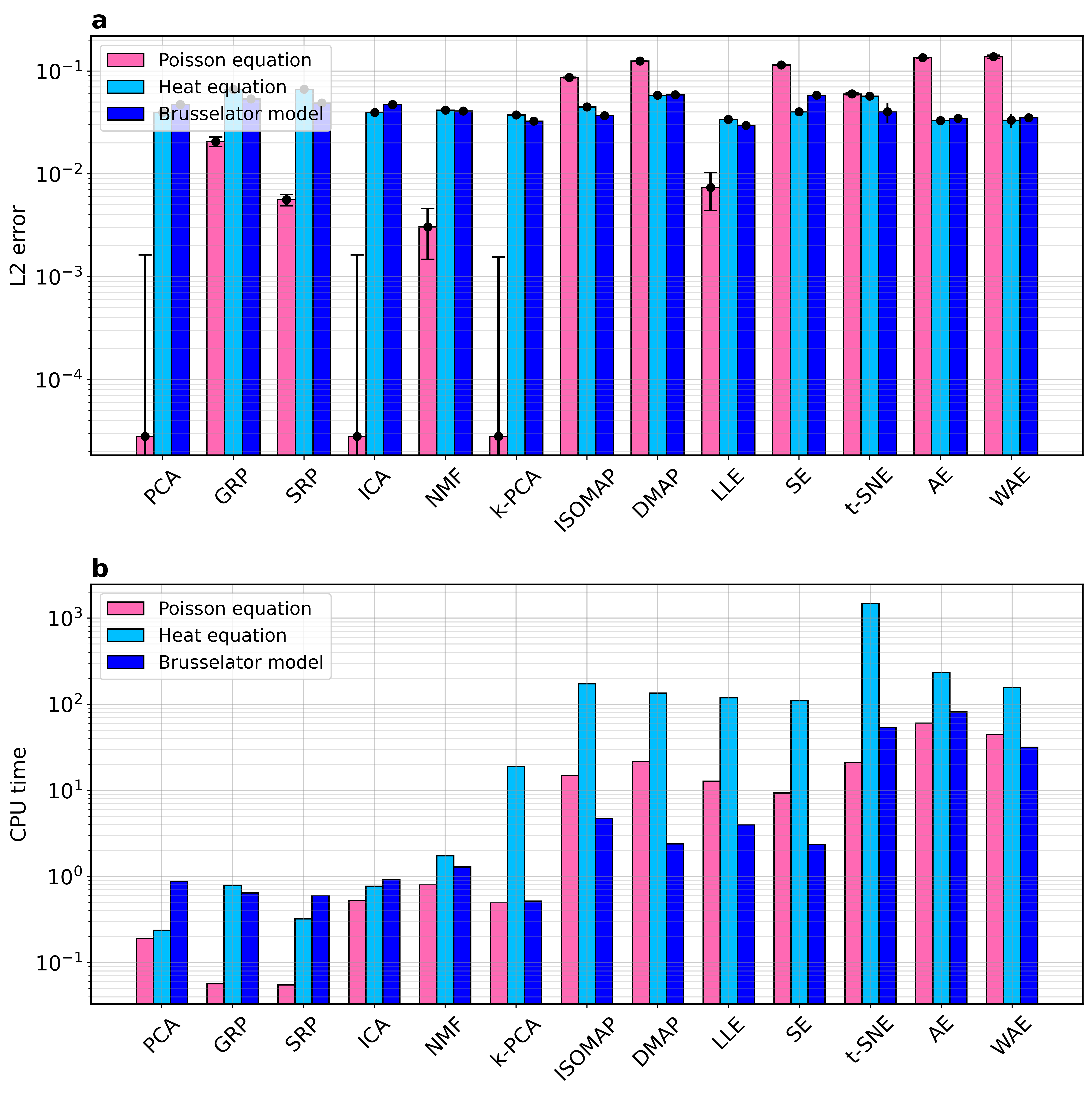
Figure 14: Overall comparison between the thirteen DR methods in terms of (a) relative error (with error bars corresponding to one standard deviation) and (b) CPU time of surrogate training. Pink bars represent the Poisson equation, blue bars the heat equation and dark blue bars the Brusselator model

In this Section, we compare the performance of all DR methods in terms of the predictive ability of the PCE surrogate. In Figure 14, we present the (a) average relative $L_{2}$ error for all thirteen DR methods and (b) the CPU time in two bar graphs. As discussed in previous sections, simple methods such as PCA and ICA performed best for the 1D Poisson equation when considering both CPU time and surrogate accuracy. This is expected given the relative simplicity of the random field expansion. For more complex problems (complexity stems from both the nature of input stochastic fields or/and the model itself) like the heat equation or the Brusselator model, nonlinear methods such as AE or LLE performed very well in reducing the stochastic input dimension for accurate PCE. One important finding is that, when CPU time is of importance, simpler methods such as PCA, k-PCA and ICA were able to result in both good accuracy and fast training. Figure 14(b), clearly shows an upward trend in CPU time as the DR method gets more complicated (nonlinear, non-convex) that can result in up to 4 orders of magnitude higher expense compared to simple methods. A key takeaway from this comparative study is to start simple. During the past few years there has been a trend in employing overly complex and overparameterized techniques (e.g., DNNs) to approximate ODEs and PDEs that could simply be emulated with simpler methods as presented in this work. As shown, such methods can be employed both for predictive analysis and probabilistic modeling (uncertainty propagation, moment estimation). One should resort to more advanced methods only when complexity of the system necessitates and simple methods fail to result in satisfactory predictive accuracy.

5 Discussion

Dimensionality reduction, an unsupervised learning task, has been established as a powerful pre-processing tool in cases where the high dimensionality of data would otherwise lead to burdensome computations. Within the context of high-dimensional UQ, only a few methods have been employed for the projection of inputs onto lower-dimensional embeddings for the construction of surrogates that enable inexpensive MC simulations and therefore UQ tasks, such as moment estimation and uncertainty propagation. Furthermore, the appropriateness of each method for various types of physics-based problems has not been investigated. In this work, we explored the functionalities, advantages and limitations associated with various DR methods applied for high-dimensional UQ in black-box-type models. The process of mapping a set of high-dimensional data to a low-dimensional compressed representation possesses numerous challenges. The selection of a suitable method according to the type of data is the most important issue that needs to be addressed.

In this work, the methods used to generate high-dimensional input stochastic fields (KLE, SRM) result in both compact and less compact representations, allowing the discovery of a latent space with low-to-medium dimensionality. The comparative analysis revealed that, for simple problems simulated on 1D domains, linear methods outperformed the more sophisticated nonlinear ones in terms of prediction accuracy, with the additional advantage of a very fast training. For more complicated problems, e.g. ones with input stochastic fields of varying lengthscales where the goal is to predict the model response in both space and time, nonlinear methods outperformed linear ones, with the downside of being more CPU-intensive, in particular exceeding the cost of linear methods from 1 to 3 orders of magnitude. In most cases, the optimal surrogate is constructed with a very small maximum polynomial degree $(s_{max}=2-4)$, indicating the ability of DR methods to reveal a smooth underlying embedding which can be mapped to responses via a lower-order polynomial expansion. Interestingly, when both predictive accuracy and CPU time are considered, simple methods such as PCA, k-PCA and ICA often outperformed the more complex and sophisticated approaches. Importantly, our results indicate that even for complex physics-based applications with high-dimensional input uncertainties, the m-PCE approach can be employed with simple DR algorithms and achieve comparable predictive accuracy to those of much more expensive surrogate modeling approaches proposed in the literature. For example, a combination of a standard PCA for DR of stochastic inputs and PCE for surrogate modeling performs as well as the use of expensive DNNs used for both the DR and surrogate modeling tasks proposed in [88], but with a training time in the order of seconds (see the test case investigated in Section 4.3). Within the context of physics-based modeling and UQ, we showed that the m-PCE approach can provide a cost-effective solution for surrogate modeling and propagation of uncertainties in both simple and complex physics-based problems.

We found that the predictive ability of the surrogate is based on both the complexity of the input-output mapping and the existence of a low-dimensional embedding of input uncertain data. Admittedly, there will be cases where high-dimensional inputs do not possess a low-dimensional structure that can be revealed with a DR method. In cases where the intrinsic dimensionality of input data is very high (e.g., for stochastic fields with small lengthscales generated with the spectral representation method, see example in Section 4.2), the construction of a PCE surrogate may be intractable. On the other hand, if a number of critical features are neglected to achieve a lower input dimensionality, the resulting embedding will not preserve the variance and local structure of the original data which will lead to the construction of an inefficient mapping between inputs and QoIs. These limitations form challenges to be addressed in future work. We anticipate that this study will assist researchers in the process of selecting suitable DR techniques for enhancing predictive analysis and UQ and alleviate the curse of dimensionality in complex problems associated with high-dimensional uncertainties.

6 Acknowledgements

This material is based upon work supported by the U.S. Department of Energy, Office of Science, Office of Advanced Scientific Computing Research under Award Number DE-SC0020428. D. Loukrezis acknowledges the support of the Graduate School Computational Engineering within the Centre for Computational Engineering at the Technische Universität Darmstadt.

References

- Der Kiureghian and Ditlevsen [2009] Armen Der Kiureghian and Ove Ditlevsen. Aleatory or epistemic? does it matter? Structural Safety, 31(2):105–112, 2009.
- Sullivan [2015] Timothy John Sullivan. Introduction to uncertainty quantification, volume 63. Springer, 2015.
- Metropolis et al. [1987] Nicholas Metropolis et al. The beginning of the monte carlo method. Los Alamos Science, 15(584):125–130, 1987.
- Liu and Liu [2001] Jun S Liu and Jun S Liu. Monte Carlo strategies in scientific computing, volume 10. Springer, 2001.
- McKay et al. [2000] Michael D McKay, Richard J Beckman, and William J Conover. A comparison of three methods for selecting values of input variables in the analysis of output from a computer code. Technometrics, 42(1):55–61, 2000.
- Helton and Davis [2003] Jon C Helton and Freddie Joe Davis. Latin hypercube sampling and the propagation of uncertainty in analyses of complex systems. Reliability Engineering & System Safety, 81(1):23–69, 2003.
- Shields and Zhang [2016] Michael D Shields and Jiaxin Zhang. The generalization of latin hypercube sampling. Reliability Engineering & System Safety, 148:96–108, 2016.
- Tokdar and Kass [2010] Surya T Tokdar and Robert E Kass. Importance sampling: a review. Wiley Interdisciplinary Reviews: Computational Statistics, 2(1):54–60, 2010.
- Gorodetsky et al. [2020] Alex A Gorodetsky, Gianluca Geraci, Michael S Eldred, and John D Jakeman. A generalized approximate control variate framework for multifidelity uncertainty quantification. Journal of Computational Physics, 408:109257, 2020.
- Peherstorfer et al. [2016] Benjamin Peherstorfer, Karen Willcox, and Max Gunzburger. Optimal model management for multifidelity monte carlo estimation. SIAM Journal on Scientific Computing, 38(5):A3163–A3194, 2016.
- Peherstorfer et al. [2018] Benjamin Peherstorfer, Philip S Beran, and Karen E Willcox. Multifidelity monte carlo estimation for large-scale uncertainty propagation. In 2018 AIAA Non-Deterministic Approaches Conference, page 1660, 2018.
- Giles [2015] Michael B Giles. Multilevel monte carlo methods. Acta Numerica, 24:259–328, 2015.
- Krumscheid et al. [2020] Sebastian Krumscheid, Fabio Nobile, and M Pisaroni. Quantifying uncertain system outputs via the multilevel monte carlo method—part i: Central moment estimation. Journal of Computational Physics, 414:109466, 2020.
- Scheichl et al. [2017] Robert Scheichl, Andrew M Stuart, and Aretha L Teckentrup. Quasi-monte carlo and multilevel monte carlo methods for computing posterior expectations in elliptic inverse problems. SIAM/ASA Journal on Uncertainty Quantification, 5(1):493–518, 2017.
- Sudret et al. [2017] Bruno Sudret, Stefano Marelli, and Joe Wiart. Surrogate models for uncertainty quantification: An overview. In 2017 11th European conference on antennas and propagation (EUCAP), pages 793–797. IEEE, 2017.
- Bhosekar and Ierapetritou [2018] Atharv Bhosekar and Marianthi Ierapetritou. Advances in surrogate based modeling, feasibility analysis, and optimization: A review. Computers & Chemical Engineering, 108:250–267, 2018.
- Rasmussen [2003] Carl Edward Rasmussen. Gaussian processes in machine learning. In Summer school on machine learning, pages 63–71. Springer, 2003.
- Bilionis and Zabaras [2012] Ilias Bilionis and Nicholas Zabaras. Multi-output local gaussian process regression: Applications to uncertainty quantification. Journal of Computational Physics, 231(17):5718–5746, 2012.
- Chen et al. [2015] Peng Chen, Nicholas Zabaras, and Ilias Bilionis. Uncertainty propagation using infinite mixture of gaussian processes and variational bayesian inference. Journal of Computational Physics, 284:291–333, 2015.
- Tripathy et al. [2016] Rohit Tripathy, Ilias Bilionis, and Marcial Gonzalez. Gaussian processes with built-in dimensionality reduction: Applications to high-dimensional uncertainty propagation. Journal of Computational Physics, 321:191–223, 2016.
- Raissi et al. [2018] Maziar Raissi, Paris Perdikaris, and George Em Karniadakis. Numerical gaussian processes for time-dependent and nonlinear partial differential equations. SIAM Journal on Scientific Computing, 40(1):A172–A198, 2018.
- Radaideh and Kozlowski [2020] Majdi I Radaideh and Tomasz Kozlowski. Surrogate modeling of advanced computer simulations using deep gaussian processes. Reliability Engineering & System Safety, 195:106731, 2020.
- Giovanis and Shields [2020] Dimitris G Giovanis and Michael D Shields. Data-driven surrogates for high dimensional models using gaussian process regression on the grassmann manifold. Computer Methods in Applied Mechanics and Engineering, 370:113269, 2020.
- Kontolati et al. [2021a] Katiana Kontolati, Darius Alix-Williams, Nicholas M Boffi, Michael L Falk, Chris H Rycroft, and Michael D Shields. Manifold learning for coarse-graining atomistic simulations: Application to amorphous solids. Acta Materialia, page 117008, 2021a.
- Ghanem and Spanos [1990] Roger Ghanem and Pol D Spanos. Polynomial chaos in stochastic finite elements. Journal of Applied Mechanics, 1990.
- Xiu and Karniadakis [2002] Dongbin Xiu and George Em Karniadakis. The wiener–askey polynomial chaos for stochastic differential equations. SIAM Journal on Scientific Computing, 24(2):619–644, 2002.
- Witteveen and Bijl [2006] Jeroen AS Witteveen and Hester Bijl. Modeling arbitrary uncertainties using gram-schmidt polynomial chaos. In 44th AIAA aerospace sciences meeting and exhibit, page 896, 2006.
- Oladyshkin and Nowak [2012] Sergey Oladyshkin and Wolfgang Nowak. Data-driven uncertainty quantification using the arbitrary polynomial chaos expansion. Reliability Engineering & System Safety, 106:179–190, 2012.
- Zheng et al. [2015] Mengdi Zheng, Xiaoliang Wan, and George Em Karniadakis. Adaptive multi-element polynomial chaos with discrete measure: Algorithms and application to spdes. Applied Numerical Mathematics, 90:91–110, 2015.
- Kontolati et al. [2021b] Katiana Kontolati, Dimitrios Loukrezis, Ketson RM dos Santos, Dimitrios G Giovanis, and Michael D Shields. Manifold learning-based polynomial chaos expansions for high-dimensional surrogate models. arXiv preprint arXiv:2107.09814, 2021b.
- Psichogios and Ungar [1992] Dimitris C Psichogios and Lyle H Ungar. A hybrid neural network-first principles approach to process modeling. AIChE Journal, 38(10):1499–1511, 1992.
- Lagaris et al. [1998] Isaac E Lagaris, Aristidis Likas, and Dimitrios I Fotiadis. Artificial neural networks for solving ordinary and partial differential equations. IEEE Transactions on Neural Networks, 9(5):987–1000, 1998.
- Zhu and Zabaras [2018] Yinhao Zhu and Nicholas Zabaras. Bayesian deep convolutional encoder–decoder networks for surrogate modeling and uncertainty quantification. Journal of Computational Physics, 366:415–447, 2018.
- Zhang et al. [2019] Dongkun Zhang, Lu Lu, Ling Guo, and George Em Karniadakis. Quantifying total uncertainty in physics-informed neural networks for solving forward and inverse stochastic problems. Journal of Computational Physics, 397:108850, 2019.
- Winovich et al. [2019] Nick Winovich, Karthik Ramani, and Guang Lin. Convpde-uq: Convolutional neural networks with quantified uncertainty for heterogeneous elliptic partial differential equations on varied domains. Journal of Computational Physics, 394:263–279, 2019.
- Yang and Perdikaris [2019] Yibo Yang and Paris Perdikaris. Adversarial uncertainty quantification in physics-informed neural networks. Journal of Computational Physics, 394:136–152, 2019.
- Raissi et al. [2019] Maziar Raissi, Paris Perdikaris, and George E Karniadakis. Physics-informed neural networks: A deep learning framework for solving forward and inverse problems involving nonlinear partial differential equations. Journal of Computational Physics, 378:686–707, 2019.
- Olivier et al. [2021] Audrey Olivier, Michael D Shields, and Lori Graham-Brady. Bayesian neural networks for uncertainty quantification in data-driven materials modeling. Computer Methods in Applied Mechanics and Engineering, 386:114079, 2021.
- Lu et al. [2021] Lu Lu, Pengzhan Jin, Guofei Pang, Zhongqiang Zhang, and George Em Karniadakis. Learning nonlinear operators via deeponet based on the universal approximation theorem of operators. Nature Machine Intelligence, 3(3):218–229, 2021.
- Goswami et al. [2021] Somdatta Goswami, Minglang Yin, Yue Yu, and George Karniadakis. A physics-informed variational deeponet for predicting the crack path in brittle materials. arXiv preprint arXiv:2108.06905, 2021.
- Gao and Ng [2021] Yihang Gao and Michael K Ng. Wasserstein generative adversarial uncertainty quantification in physics-informed neural networks. arXiv preprint arXiv:2108.13054, 2021.
- Kontolati et al. [2022] Katiana Kontolati, Somdatta Goswami, Michael D Shields, and George Em Karniadakis. On the influence of over-parameterization in manifold based surrogates and deep neural operators. arXiv preprint arXiv:2203.05071, 2022.
- Keogh and Mueen [2017] Eamonn J Keogh and Abdullah Mueen. Curse of dimensionality. Encyclopedia of machine learning and data mining, 2017:314–315, 2017.
- Lüthen et al. [2021] Nora Lüthen, Stefano Marelli, and Bruno Sudret. Sparse polynomial chaos expansions: Literature survey and benchmark. SIAM/ASA Journal on Uncertainty Quantification, 9(2):593–649, 2021.
- Lüthen et al. [2020] Nora Lüthen, Stefano Marelli, and Bruno Sudret. A benchmark of basis-adaptive sparse polynomial chaos expansions for engineering regression problems. arXiv preprint arXiv:2009.04800, 2020.
- Tiripeddy and Ghanem [2014] Ramakrinsha Tiripeddy and Roger Ghanem. Basis adaptation in homogeneous chaos spaces. Journal of Computational Physics, 259:304–317, 2014.
- Thimmisetty et al. [2017] Charanraj Thimmisetty, Panagiotis Tsilifis, and Roger Ghanem. Homogeneous chaos basis adaptation for design optimization under uncertainty: Application to the oil well placement problem. Ai Edam, 31(3):265–276, 2017.
- Ghauch et al. [2019] Ziad G Ghauch, Venkat Aitharaju, William R Rodgers, Praveen Pasupuleti, Arnaud Dereims, and Roger G Ghanem. Integrated stochastic analysis of fiber composites manufacturing using adapted polynomial chaos expansions. Composites Part A: Applied Science and Manufacturing, 118:179–193, 2019.
- Tsilifis and Ghanem [2017] Panagiotis Tsilifis and Roger G Ghanem. Reduced wiener chaos representation of random fields via basis adaptation and projection. Journal of Computational Physics, 341:102–120, 2017.
- Tsilifis et al. [2019] Panagiotis Tsilifis, Xun Huan, Cosmin Safta, Khachik Sargsyan, Guilhem Lacaze, Joseph C Oefelein, Habib N Najm, and Roger G Ghanem. Compressive sensing adaptation for polynomial chaos expansions. Journal of Computational Physics, 380:29–47, 2019.
- Kougioumtzoglou et al. [2020] Ioannis A Kougioumtzoglou, Ioannis Petromichelakis, and Apostolos F Psaros. Sparse representations and compressive sampling approaches in engineering mechanics: A review of theoretical concepts and diverse applications. Probabilistic Engineering Mechanics, 61:103082, 2020.
- Hampton and Doostan [2018] Jerrad Hampton and Alireza Doostan. Basis adaptive sample efficient polynomial chaos (base-pc). Journal of Computational Physics, 371:20–49, 2018.
- Zeng et al. [2021] Xiaoshu Zeng, John Red-Horse, and Roger Ghanem. Accelerated basis adaptation in homogeneous chaos spaces. Computer Methods in Applied Mechanics and Engineering, 386:114109, 2021.
- Papaioannou et al. [2019] Iason Papaioannou, Max Ehre, and Daniel Straub. Pls-based adaptation for efficient pce representation in high dimensions. Journal of Computational Physics, 387:186–204, 2019.
- Zhou et al. [2020] Yicheng Zhou, Zhenzhou Lu, Jinghan Hu, and Yingshi Hu. Surrogate modeling of high-dimensional problems via data-driven polynomial chaos expansions and sparse partial least square. Computer Methods in Applied Mechanics and Engineering, 364:112906, 2020.
- Ehre et al. [2021] Max Ehre, Iason Papaioannou, Bruno Sudret, and Daniel Straub. Sequential active learning of low-dimensional model representations for reliability analysis. arXiv preprint arXiv:2106.04453, 2021.
- Blatman and Sudret [2010] Géraud Blatman and Bruno Sudret. An adaptive algorithm to build up sparse polynomial chaos expansions for stochastic finite element analysis. Probabilistic Engineering Mechanics, 25(2):183–197, 2010.
- Pan and Dias [2017] Qiujing Pan and Daniel Dias. Sliced inverse regression-based sparse polynomial chaos expansions for reliability analysis in high dimensions. Reliability Engineering & System Safety, 167:484–493, 2017.
- Loukrezis et al. [2020] Dimitrios Loukrezis, Armin Galetzka, and Herbert De Gersem. Robust adaptive least squares polynomial chaos expansions in high-frequency applications. International Journal of Numerical Modelling: Electronic Networks, Devices and Fields, 33(6):e2725, 2020.
- Jakeman et al. [2017] John D Jakeman, Akil Narayan, and Tao Zhou. A generalized sampling and preconditioning scheme for sparse approximation of polynomial chaos expansions. SIAM Journal on Scientific Computing, 39(3):A1114–A1144, 2017.
- Salehi et al. [2018] Saeed Salehi, Mehrdad Raisee, Michel J Cervantes, and Ahmad Nourbakhsh. An efficient multifidelity 1-minimization method for sparse polynomial chaos. Computer Methods in Applied Mechanics and Engineering, 334:183–207, 2018.
- Guo et al. [2018] Ling Guo, Akil Narayan, and Tao Zhou. A gradient enhanced 1-minimization for sparse approximation of polynomial chaos expansions. Journal of Computational Physics, 367:49–64, 2018.
- Rauhut and Ward [2012] Holger Rauhut and Rachel Ward. Sparse legendre expansions via 1-minimization. Journal of Approximation Theory, 164(5):517–533, 2012.
- Hesterberg et al. [2008] Tim Hesterberg, Nam Hee Choi, Lukas Meier, and Chris Fraley. Least angle and 1 penalized regression: A review. Statistics Surveys, 2:61–93, 2008.
- Blatman and Sudret [2011] Géraud Blatman and Bruno Sudret. Adaptive sparse polynomial chaos expansion based on least angle regression. Journal of Computational Physics, 230(6):2345–2367, 2011.
- Man et al. [2021] Jun Man, Guang Lin, Yijun Yao, and Lingzao Zeng. A generalized multi-fidelity simulation method using sparse polynomial chaos expansion. Journal of Computational and Applied Mathematics, 397:113613, 2021.
- Meng and Li [2017] Jin Meng and Heng Li. An efficient stochastic approach for flow in porous media via sparse polynomial chaos expansion constructed by feature selection. Advances in Water Resources, 105:13–28, 2017.
- Meng and Li [2019] Jin Meng and Heng Li. Efficient uncertainty quantification for unconfined flow in heterogeneous media with the sparse polynomial chaos expansion. Transport in Porous Media, 126(1):23–38, 2019.
- He et al. [2020] Wanxin He, Yan Zeng, and Gang Li. An adaptive polynomial chaos expansion for high-dimensional reliability analysis. Structural and Multidisciplinary Optimization, 62(4):2051–2067, 2020.
- Van Der Maaten et al. [2009] Laurens Van Der Maaten, Eric Postma, and Jaap Van den Herik. Dimensionality reduction: a comparative review. J Mach Learn Res, 10(66-71):13, 2009.
- Damianou and Lawrence [2013] Andreas Damianou and Neil D Lawrence. Deep gaussian processes. In Artificial Intelligence and Statistics, pages 207–215. PMLR, 2013.
- Calandra et al. [2016] Roberto Calandra, Jan Peters, Carl Edward Rasmussen, and Marc Peter Deisenroth. Manifold gaussian processes for regression. In 2016 International Joint Conference on Neural Networks (IJCNN), pages 3338–3345. IEEE, 2016.
- Constantine [2015] Paul G Constantine. Active subspaces: Emerging ideas for dimension reduction in parameter studies. SIAM, 2015.
- Constantine and Gleich [2014] Paul Constantine and David Gleich. Computing active subspaces with monte carlo. arXiv preprint arXiv:1408.0545, 2014.
- Constantine et al. [2015] Paul Constantine, Michael Emory, Johan Larsson, and Gianluca Iaccarino. Exploiting active subspaces to quantify uncertainty in the numerical simulation of the hyshot ii scramjet. Journal of Computational Physics, 302:1–20, 2015.
- Lataniotis et al. [2020] Christos Lataniotis, Stefano Marelli, and Bruno Sudret. Extending classical surrogate modeling to high dimensions through supervised dimensionality reduction: a data-driven approach. International Journal for Uncertainty Quantification, 10(1), 2020.
- Doostan et al. [2013] Alireza Doostan, AbdoulAhad Validi, and Gianluca Iaccarino. Non-intrusive low-rank separated approximation of high-dimensional stochastic models. Computer Methods in Applied Mechanics and Engineering, 263:42–55, 2013.
- Konakli and Sudret [2016] Katerina Konakli and Bruno Sudret. Reliability analysis of high-dimensional models using low-rank tensor approximations. Probabilistic Engineering Mechanics, 46:18–36, 2016.
- Bigoni et al. [2016] Daniele Bigoni, Allan P Engsig-Karup, and Youssef M Marzouk. Spectral tensor-train decomposition. SIAM Journal on Scientific Computing, 38(4):A2405–A2439, 2016.
- Gorodetsky and Jakeman [2018] Alex A Gorodetsky and John D Jakeman. Gradient-based optimization for regression in the functional tensor-train format. Journal of Computational Physics, 374:1219–1238, 2018.
- He and Zhang [2020] Zichang He and Zheng Zhang. High-dimensional uncertainty quantification via active and rank-adaptive tensor regression. In 2020 IEEE 29th Conference on Electrical Performance of Electronic Packaging and Systems (EPEPS), pages 1–3. IEEE, 2020.
- Hinton and Salakhutdinov [2006] Geoffrey E Hinton and Ruslan R Salakhutdinov. Reducing the dimensionality of data with neural networks. science, 313(5786):504–507, 2006.
- Huang et al. [2015] Wenbing Huang, Deli Zhao, Fuchun Sun, Huaping Liu, and Edward Chang. Scalable gaussian process regression using deep neural networks. In Twenty-fourth international joint conference on artificial intelligence, 2015.
- Li and Wang [2020] Mingyang Li and Zequn Wang. Deep learning for high-dimensional reliability analysis. Mechanical Systems and Signal Processing, 139:106399, 2020.
- Khoo et al. [2021] Yuehaw Khoo, Jianfeng Lu, and Lexing Ying. Solving parametric pde problems with artificial neural networks. European Journal of Applied Mathematics, 32(3):421–435, 2021.
- Boncoraglio and Farhat [2021] Gabriele Boncoraglio and Charbel Farhat. Active manifold and model-order reduction to accelerate multidisciplinary analysis and optimization. AIAA Journal, 59(11):4739–4753, 2021.
- Zhu et al. [2019] Yinhao Zhu, Nicholas Zabaras, Phaedon-Stelios Koutsourelakis, and Paris Perdikaris. Physics-constrained deep learning for high-dimensional surrogate modeling and uncertainty quantification without labeled data. Journal of Computational Physics, 394:56–81, 2019.
- Tripathy and Bilionis [2018] Rohit K Tripathy and Ilias Bilionis. Deep uq: Learning deep neural network surrogate models for high dimensional uncertainty quantification. Journal of computational physics, 375:565–588, 2018.
- Guo et al. [2022] Ling Guo, Hao Wu, and Tao Zhou. Normalizing field flows: Solving forward and inverse stochastic differential equations using physics-informed flow models. Journal of Computational Physics, page 111202, 2022.
- Gao et al. [2017] Lianli Gao, Jingkuan Song, Xingyi Liu, Junming Shao, Jiajun Liu, and Jie Shao. Learning in high-dimensional multimedia data: the state of the art. Multimedia Systems, 23(3):303–313, 2017.
- Chandrashekar and Sahin [2014] Girish Chandrashekar and Ferat Sahin. A survey on feature selection methods. Computers & Electrical Engineering, 40(1):16–28, 2014.
- Cunningham and Ghahramani [2015] John P Cunningham and Zoubin Ghahramani. Linear dimensionality reduction: Survey, insights, and generalizations. The Journal of Machine Learning Research, 16(1):2859–2900, 2015.
- Gite et al. [2018] Hanumant R Gite, Mahesh M Solankar, Rupali R Surase, and Karbhari V Kale. Comparative study and analysis of dimensionality reduction techniques for hyperspectral data. In International Conference on Recent Trends in Image Processing and Pattern Recognition, pages 534–546. Springer, 2018.
- Sellami and Farah [2018] Akrem Sellami and Mohamed Farah. Comparative study of dimensionality reduction methods for remote sensing images interpretation. In 2018 4th International Conference on Advanced Technologies for Signal and Image Processing (ATSIP), pages 1–6. IEEE, 2018.
- Konstorum et al. [2018] Anna Konstorum, Nathan Jekel, Emily Vidal, and Reinhard Laubenbacher. Comparative analysis of linear and nonlinear dimension reduction techniques on mass cytometry data. bioRxiv, page 273862, 2018.
- Ayesha et al. [2020] Shaeela Ayesha, Muhammad Kashif Hanif, and Ramzan Talib. Overview and comparative study of dimensionality reduction techniques for high dimensional data. Information Fusion, 59:44–58, 2020.
- Alkhayrat et al. [2020] Maha Alkhayrat, Mohamad Aljnidi, and Kadan Aljoumaa. A comparative dimensionality reduction study in telecom customer segmentation using deep learning and pca. Journal of Big Data, 7(1):1–23, 2020.
- Lataniotis [2019] Christos Lataniotis. Data-driven uncertainty quantification for high-dimensional engineering problems. PhD thesis, ETH Zurich, 2019.
- Olivier et al. [2020] Audrey Olivier, Dimitrios Giovanis, BS Aakash, Mohit Chauhan, Lohit Vandanapu, and Michael D Shields. Uqpy: A general purpose python package and development environment for uncertainty quantification. Journal of Computational Science, 47:101204, 2020.
- Pedregosa et al. [2011] F. Pedregosa, G. Varoquaux, A. Gramfort, V. Michel, B. Thirion, O. Grisel, M. Blondel, P. Prettenhofer, R. Weiss, V. Dubourg, J. Vanderplas, A. Passos, D. Cournapeau, M. Brucher, M. Perrot, and E. Duchesnay. Scikit-learn: Machine learning in Python. Journal of Machine Learning Research, 12:2825–2830, 2011.
- Fodor [2002] Imola K Fodor. A survey of dimension reduction techniques. Technical report, Citeseer, 2002.
- De Lathauwer et al. [2000] Lieven De Lathauwer, Bart De Moor, and Joos Vandewalle. A multilinear singular value decomposition. SIAM journal on Matrix Analysis and Applications, 21(4):1253–1278, 2000.
- Huang et al. [2001] SP Huang, ST Quek, and KK Phoon. Convergence study of the truncated karhunen–loeve expansion for simulation of stochastic processes. International Journal for Numerical Methods in Engineering, 52(9):1029–1043, 2001.
- Bingham and Mannila [2001] Ella Bingham and Heikki Mannila. Random projection in dimensionality reduction: applications to image and text data. In Proceedings of the seventh ACM SIGKDD international conference on Knowledge discovery and data mining, pages 245–250, 2001.
- Goel et al. [2005] Navin Goel, George Bebis, and Ara Nefian. Face recognition experiments with random projection. In Biometric Technology for Human Identification II, volume 5779, pages 426–437. International Society for Optics and Photonics, 2005.
- Cannings and Samworth [2017] Timothy I Cannings and Richard J Samworth. Random-projection ensemble classification. Journal of the Royal Statistical Society: Series B (Statistical Methodology), 79(4):959–1035, 2017.
- Xu et al. [2017] Chugui Xu, Ju Ren, Yaoxue Zhang, Zhan Qin, and Kui Ren. Dppro: Differentially private high-dimensional data release via random projection. IEEE Transactions on Information Forensics and Security, 12(12):3081–3093, 2017.
- Dasgupta and Gupta [1999] Sanjoy Dasgupta and Anupam Gupta. An elementary proof of the johnson-lindenstrauss lemma. International Computer Science Institute, Technical Report, 22(1):1–5, 1999.
- Achlioptas [2001] Dimitris Achlioptas. Database-friendly random projections. In Proceedings of the twentieth ACM SIGMOD-SIGACT-SIGART symposium on Principles of database systems, pages 274–281, 2001.
- Sun et al. [2021] Yiming Sun, Yang Guo, Joel A Tropp, and Madeleine Udell. Tensor random projection for low memory dimension reduction. arXiv preprint arXiv:2105.00105, 2021.
- Saul et al. [2006] Lawrence K Saul, Kilian Q Weinberger, Fei Sha, Jihun Ham, and Daniel D Lee. Spectral methods for dimensionality reduction. Semi-supervised learning, 3, 2006.
- Schölkopf et al. [1997] Bernhard Schölkopf, Alexander Smola, and Klaus-Robert Müller. Kernel principal component analysis. In International conference on artificial neural networks, pages 583–588. Springer, 1997.
- Hoffmann [2007] Heiko Hoffmann. Kernel pca for novelty detection. Pattern Recognition, 40(3):863–874, 2007.
- Mika et al. [1998] Sebastian Mika, Bernhard Schölkopf, Alexander J Smola, Klaus-Robert Müller, Matthias Scholz, and Gunnar Rätsch. Kernel pca and de-noising in feature spaces. In NIPS, volume 11, pages 536–542, 1998.
- Bishop [2006] Christopher M Bishop. Pattern recognition and machine learning. springer, 2006.
- dos Santos et al. [2022] Ketson R dos Santos, Dimitrios G Giovanis, and Michael D Shields. Grassmannian diffusion maps–based dimension reduction and classification for high-dimensional data. SIAM Journal on Scientific Computing, 44(2):B250–B274, 2022.
- Tenenbaum et al. [2000] Joshua B Tenenbaum, Vin De Silva, and John C Langford. A global geometric framework for nonlinear dimensionality reduction. Science, 290(5500):2319–2323, 2000.
- Cox and Cox [2008] Michael AA Cox and Trevor F Cox. Multidimensional scaling. In Handbook of data visualization, pages 315–347. Springer, 2008.
- Floyd [1962] Robert W Floyd. Algorithm 97: shortest path. Communications of the ACM, 5(6):345, 1962.
- Dijkstra et al. [1959] Edsger W Dijkstra et al. A note on two problems in connexion with graphs. Numerische mathematik, 1(1):269–271, 1959.
- Coifman and Lafon [2006] Ronald R Coifman and Stéphane Lafon. Diffusion maps. Applied and Computational Harmonic Analysis, 21(1):5–30, 2006.
- Lafon and Lee [2006] Stephane Lafon and Ann B Lee. Diffusion maps and coarse-graining: A unified framework for dimensionality reduction, graph partitioning, and data set parameterization. IEEE Transactions on Pattern Analysis and Machine Intelligence, 28(9):1393–1403, 2006.
- Singer and Wu [2012] Amit Singer and H-T Wu. Vector diffusion maps and the connection laplacian. Communications on pure and applied mathematics, 65(8):1067–1144, 2012.
- dos Santos et al. [2021] Ketson RM dos Santos, Dimitrios G Giovanis, Katiana Kontolati, Dimitrios Loukrezis, and Michael D Shields. Grassmannian diffusion maps based surrogate modeling via geometric harmonics. arXiv preprint arXiv:2109.13805, 2021.
- Roweis and Saul [2000] Sam T Roweis and Lawrence K Saul. Nonlinear dimensionality reduction by locally linear embedding. Science, 290(5500):2323–2326, 2000.
- Polito and Perona [2002] Marzia Polito and Pietro Perona. Grouping and dimensionality reduction by locally linear embedding. Advances in Neural Information Processing Systems, 14(2), 2002.
- Donoho and Grimes [2003] David L Donoho and Carrie Grimes. Hessian eigenmaps: Locally linear embedding techniques for high-dimensional data. Proceedings of the National Academy of Sciences, 100(10):5591–5596, 2003.
- Zhang and Zha [2004] Zhenyue Zhang and Hongyuan Zha. Principal manifolds and nonlinear dimensionality reduction via tangent space alignment. SIAM journal on scientific computing, 26(1):313–338, 2004.
- Belkin and Niyogi [2003] Mikhail Belkin and Partha Niyogi. Laplacian eigenmaps for dimensionality reduction and data representation. Neural computation, 15(6):1373–1396, 2003.
- Pal et al. [2013] Madhab Pal, Rajib Roy, Joyanta Basu, and Milton S Bepari. Blind source separation: A review and analysis. In 2013 International Conference Oriental COCOSDA held jointly with 2013 Conference on Asian Spoken Language Research and Evaluation (O-COCOSDA/CASLRE), pages 1–5. IEEE, 2013.
- Qian et al. [2018] Yan-min Qian, Chao Weng, Xuan-kai Chang, Shuai Wang, and Dong Yu. Past review, current progress, and challenges ahead on the cocktail party problem. Frontiers of Information Technology & Electronic Engineering, 19(1):40–63, 2018.
- Hyvärinen and Oja [2000] Aapo Hyvärinen and Erkki Oja. Independent component analysis: algorithms and applications. Neural Networks, 13(4-5):411–430, 2000.
- Hyvärinen and Oja [1997] Aapo Hyvärinen and Erkki Oja. A fast fixed-point algorithm for independent component analysis. Neural Computation, 9(7):1483–1492, 1997.
- Bingham and Hyvärinen [2000] Ella Bingham and Aapo Hyvärinen. A fast fixed-point algorithm for independent component analysis of complex valued signals. International journal of neural systems, 10(01):1–8, 2000.
- Hyvarinen [1999] Aapo Hyvarinen. Fast and robust fixed-point algorithms for independent component analysis. IEEE transactions on Neural Networks, 10(3):626–634, 1999.
- Paatero and Tapper [1994] Pentti Paatero and Unto Tapper. Positive matrix factorization: A non-negative factor model with optimal utilization of error estimates of data values. Environmetrics, 5(2):111–126, 1994.
- Wang and Zhang [2012] Yu-Xiong Wang and Yu-Jin Zhang. Nonnegative matrix factorization: A comprehensive review. IEEE Transactions on knowledge and data engineering, 25(6):1336–1353, 2012.
- Lee and Seung [1999] Daniel D Lee and H Sebastian Seung. Learning the parts of objects by non-negative matrix factorization. Nature, 401(6755):788–791, 1999.
- Févotte and Idier [2011] Cédric Févotte and Jérôme Idier. Algorithms for nonnegative matrix factorization with the -divergence. Neural Computation, 23(9):2421–2456, 2011.
- Eggert and Korner [2004] Julian Eggert and Edgar Korner. Sparse coding and nmf. In 2004 IEEE International Joint Conference on Neural Networks (IEEE Cat. No. 04CH37541), volume 4, pages 2529–2533. IEEE, 2004.
- Van der Maaten and Hinton [2008] Laurens Van der Maaten and Geoffrey Hinton. Visualizing data using t-sne. Journal of Machine Learning Research, 9(11), 2008.
- Van Der Maaten [2014] Laurens Van Der Maaten. Accelerating t-sne using tree-based algorithms. The Journal of Machine Learning Research, 15(1):3221–3245, 2014.
- Chen and Chen [1995] Tianping Chen and Hong Chen. Universal approximation to nonlinear operators by neural networks with arbitrary activation functions and its application to dynamical systems. IEEE Transactions on Neural Networks, 6(4):911–917, 1995.
- Rossi and Conan-Guez [2005] Fabrice Rossi and Brieuc Conan-Guez. Functional multi-layer perceptron: a non-linear tool for functional data analysis. Neural Networks, 18(1):45–60, 2005.
- Bank et al. [2020] Dor Bank, Noam Koenigstein, and Raja Giryes. Autoencoders. arXiv preprint arXiv:2003.05991, 2020.
- Rumelhart et al. [1985] David E Rumelhart, Geoffrey E Hinton, and Ronald J Williams. Learning internal representations by error propagation. Technical report, California Univ San Diego La Jolla Inst for Cognitive Science, 1985.
- Baldi [2012] Pierre Baldi. Autoencoders, unsupervised learning, and deep architectures. In Proceedings of ICML workshop on unsupervised and transfer learning, pages 37–49. JMLR Workshop and Conference Proceedings, 2012.
- Kingma and Welling [2013] Diederik P Kingma and Max Welling. Auto-encoding variational bayes. arXiv preprint arXiv:1312.6114, 2013.
- Kingma and Welling [2019] Diederik P Kingma and Max Welling. An introduction to variational autoencoders. arXiv preprint arXiv:1906.02691, 2019.
- Tolstikhin et al. [2017] Ilya Tolstikhin, Olivier Bousquet, Sylvain Gelly, and Bernhard Schoelkopf. Wasserstein auto-encoders. arXiv preprint arXiv:1711.01558, 2017.
- Rubenstein et al. [2018] Paul K Rubenstein, Bernhard Schoelkopf, and Ilya Tolstikhin. On the latent space of wasserstein auto-encoders. arXiv preprint arXiv:1802.03761, 2018.
- Rubner et al. [2000] Yossi Rubner, Carlo Tomasi, and Leonidas J Guibas. The earth mover’s distance as a metric for image retrieval. International Journal of Computer Vision, 40(2):99–121, 2000.
- Sorzano et al. [2014] Carlos Oscar Sánchez Sorzano, Javier Vargas, and A Pascual Montano. A survey of dimensionality reduction techniques. arXiv preprint arXiv:1403.2877, 2014.
- Soize and Ghanem [2004] Christian Soize and Roger Ghanem. Physical systems with random uncertainties: chaos representations with arbitrary probability measure. SIAM Journal on Scientific Computing, 26(2):395–410, 2004.
- Wan and Karniadakis [2006] Xiaoliang Wan and George Em Karniadakis. Beyond wiener–askey expansions: handling arbitrary pdfs. Journal of Scientific Computing, 27(1):455–464, 2006.
- Torre et al. [2019] Emiliano Torre, Stefano Marelli, Paul Embrechts, and Bruno Sudret. Data-driven polynomial chaos expansion for machine learning regression. Journal of Computational Physics, 388:601–623, 2019.
- Rosenblatt [1952] Murray Rosenblatt. Remarks on a multivariate transformation. The annals of mathematical statistics, 23(3):470–472, 1952.
- Bergstra et al. [2011] James Bergstra, Rémi Bardenet, Yoshua Bengio, and Balázs Kégl. Algorithms for hyper-parameter optimization. Advances in Neural Information Processing Systems, 24, 2011.
- Feurer and Hutter [2019] Matthias Feurer and Frank Hutter. Hyperparameter optimization. In Automated Machine Learning, pages 3–33. Springer, Cham, 2019.
- Bischl et al. [2012] Bernd Bischl, Olaf Mersmann, Heike Trautmann, and Claus Weihs. Resampling methods for meta-model validation with recommendations for evolutionary computation. Evolutionary Computation, 20(2):249–275, 2012.
- Grigoriu [1998] Mircea Grigoriu. Simulation of Stationary Non-Gaussian Translation Processes. Journal of Engineering Mechanics, 124(2):121–126, 1998. ISSN 0733-9399. doi: 10.1061/(asce)0733-9399(1998)124:2(121).
- Vaidyanathan [2015] Sundarapandian Vaidyanathan. Dynamics and control of brusselator chemical reaction. Int J ChemTech Res, 8(6):740–749, 2015.
- Shinozuka and Deodatis [1996] Masanobu Shinozuka and George Deodatis. Simulation of multi-dimensional gaussian stochastic fields by spectral representation. Applied Mechanics Reviews, 49, 1996.