Point-Level Region Contrast for Object Detection Pre-Training

Abstract

In this work we present point-level region contrast, a self-supervised pre-training approach for the task of object detection. This approach is motivated by the two key factors in detection: localization and recognition. While accurate localization favors models that operate at the pixel- or point-level, correct recognition typically relies on a more holistic, region-level view of objects. Incorporating this perspective in pre-training, our approach performs contrastive learning by directly sampling individual point pairs from different regions. Compared to an aggregated representation per region, our approach is more robust to the change in input region quality, and further enables us to implicitly improve initial region assignments via online knowledge distillation during training. Both advantages are important when dealing with imperfect regions encountered in the unsupervised setting. Experiments show point-level region contrast improves on state-of-the-art pre-training methods for object detection and segmentation across multiple tasks and datasets, and we provide extensive ablation studies and visualizations to aid understanding. Code will be made available.

1 Introduction

Un-/self-supervised learning – in particular contrastive learning [24, 20, 6] – has recently arisen as a powerful tool to obtain visual representations that can potentially benefit from an unlimited amount of unlabeled data. Promising signals are observed on important tasks like object detection [28]. For example, MoCo [20] shows convincing improvement on VOC [16] over supervised pre-training by simply learning to discriminate between images as holistic instances [14] on the ImageNet-1K dataset [37]. Since then, numerous pre-text tasks that focus on intra-image contrast have been devised specifically for object detection as the downstream transfer task [43, 51, 23]. While there has been steady progress, state-of-the-art detectors [1] still use weights from supervised pre-training (e.g., classification on ImageNet-22K [12]). The full potential of unsupervised pre-training for object detection is yet to be realized.

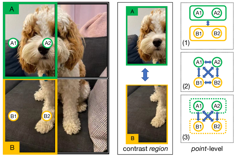
Figure 1: For intra-image contrastive learning, samples of a feature map can be aggregated and then compared between regions (1), compared directly between all samples (2), or only compared directly between samples in different regions (3). We call (3) point-level region contrast, it allows both learning at the point-level to help localization, and at the region-level to help holistic object recognition – two crucial aspects for object detection.

Object detection requires both accurate localization of objects in an image and correct recognition of their semantic categories. These two sub-tasks are tightly connected and often reinforce each other in successful detectors [32]. For example, region proposal methods [41, 54, 2] that first narrow down candidate object locations have enabled R-CNN [18] to perform classification on rich, region-level features. Conversely, today’s dominant paradigm for object instance segmentation [21] first identifies object categories along with their coarse bounding boxes, and later uses them to compute masks for better localization at the pixel-level.

With this perspective, we hypothesize that to learn a useful representation for object detection, it is also desirable to balance recognition and localization by leveraging information at various levels during pre-training. Object recognition in a scene typically takes place at the region-level [18, 35]. To support this, it is preferable to maintain a conceptually coherent ‘label’ for each region, and learn to contrast pairs of regions for representation learning. On the other hand, for better localization, the model is preferred to operate at the pixel-, or ‘point-level’ [26, 9], especially when an initial, unsupervised, assignment of pixels to regions (i.e., segmentation) is sub-optimal (see Fig. 1 for an example). To our knowledge, existing methods in this frontier can be lacking in either of these two aspects (to be discussed in Sec. 2).

In this paper, we present a self-supervised pre-training approach that conceptually contrasts at the region-level while operating at the point-level. Starting from MoCo v2 [7] as an image-level baseline, we introduce the notion of ‘regions’ by dividing each image into a non-overlapping grid [23]. Treating rectangular regions on this grid as separate instances, we can define the task of intra-image discrimination on top of the existing inter-image one [14] and pre-train a representation with contrastive objectives. Deviating from the common practice that aggregates features for contrastive learning [20, 6, 23], we directly operate at the point-level by sampling multiple points from each region, and contrasting point pairs individually across regions (see Fig. 1, right column for illustrations).

The advantage of operating at the point-level is two-fold, both concerning dealing with imperfect regions as there is no ground-truth. First, such a design can be more robust to the change in region quality, since feature aggregation can cause ambiguities when the regions are not well localized (e.g., in Fig. 1, both regions of interest can mean ‘a mixture of dog and couch’), whereas individual points still allow the model to see distinctions. Second and perhaps more importantly, it can enable us to bootstrap [19] for potentially better regions during the training process. This is because any segmentation can be viewed as a hard-coded form of point affinities – 1 for point pairs within the same region and 0 otherwise; and a natural by-product of contrasting point pairs is soft point affinities (values between 0 and 1) that implicitly encode regions. By viewing the momentum encoder as a ‘teacher’ network, we can formulate the problem as knowledge distillation one [25, 4], and improving point affinities (and thus implicitly regions) online in the same self-supervised fashion.

Empirically, we applied our approach to standard pre-training datasets (ImageNet-1K [12] and COCO train set [28]), and transferred the representation to multiple downstream datasets: VOC [16], COCO (for both object detection and instance segmentation), and Cityscapes [10] (semantic segmentation). We show strong results compared to state-of-the-art pre-training methods which use image-level, point-level, or region-level contrastive learning. Moreover, we provide extensive ablation studies covering different aspects in design, and qualitatively visualize the point affinities learned through knowledge distillation.

While we are yet to showcase improvements on larger models, longer training schedules, stronger augmentations [17], and bigger pre-training data for object detection, we believe our explorations on the pre-training design that better balances recognition and localization can inspire more works in this direction.

2 Related Work

Self-supervised learning.

Supervised learning/classification [22, 37] has been the dominant method for pre-training representations useful for downstream tasks in computer vision. Recently, contrastive learning [46, 24, 39, 20, 6, 15] has emerged as a promising alternative that pre-trains visual representations without class labels or other forms of human annotations – a paradigm commonly referred as ‘self-supervised learning’. By definition, self-supervised learning holds the potential of scaling up pre-training to huge models and billion-scale data. As a demonstration, revolutionary progress has already been made in fields like natural language processing [13, 34, 3] through scaling. For computer vision, such a moment is yet to happen. Nonetheless, object detection as a fundamental task in computer vision is a must-have benchmark to test the transferability of pre-trained representations [18].

Contrastive learning.

Akin to supervised learning which maps images to class labels, contrastive learning maps images to separate vector embeddings, and attracts positive embedding pairs while dispels negative pairs. A key concept connecting the two types of learning is instance discrimination [14], which models each image as its own class. Under this formulation, two augmentations of the same image is considered as a positive pair, while different images form negative pairs. Interestingly, recent works show that negative pairs are not required to learn meaningful representations [19, 8] for reasons are yet to be understood. Regardless, all these frameworks treat each image as a single instance and use aggregated (i.e., pooled) features to compute embeddings. Such a classification-oriented design largely ignores the internal structures of images, which could limit their application to object detection that performs dense search within an image [35, 30, 27].

Point-level contrast.

Many recent works [43, 51, 29, 50, 33] have realized the above limitation, and extended the original idea from contrasting features between whole images to contrasting features at points. Different ways to match points as pairs have been explored. For example, [43] selects positive pairs by ranking similarities among all points in the latent space; [51] defines positive pairs by spatial proximity; [29] jointly matches a set of features at points to another set via Sinkhorn-Knopp algorithm [11], designed to maximize the set-level similarity for sampled features. However, we believe directly contrasting features at arbitrary points over-weights localization, and as a result misses a more global view of the entire object that can lead to better recognition.

Region-level contrast.

Closest to our paper is the most recent line of work that contrasts representations at the region-level [23, 48, 44, 49, 47, 36]. Specifically, images are divided into regions of interest, via either external input [23, 44, 49], or sliding windows [47], or just random sampling [48, 36]. Influenced by image-level contrastive learning, most approaches represent each region with a single, aggregated vector embedding for loss computation and other operations, which we argue – and show empirically – is detrimental for localization of objects.

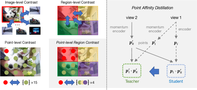
Figure 2: Illustration of point-level region contrast (Sec. 3.2), which also enables point affinity distillation (Sec. 3.3). On the left we show four different types of contrastive learning methods, including image-level, region-level, point-level and our point-level region contrast. On the right we show point affinity distillation with one pair of points.

3 Approach

In this section we detail our approach: point-level region contrast. To lay the background and introduce notations, we begin by reviewing the formulation of MoCo [20].

3.1 Background: Momentum Contrast

As the name indicates, MoCo [20, 7] is a contrastive learning framework [42, 6] that effectively uses momentum encoders to learn representations. Treating each image as a single instance to discriminate against others, MoCo operates at the image-level (see Fig. 2 top left corner).

Image-level contrast.

While the original model for instance discrimination [14] literally keeps a dedicated weight vector for each image in the dataset (on ImageNet-1K [37] it would mean more than one million vectors), modern frameworks [46, 6] formulate this task as a contrastive learning one which only requires online computation of embedding vectors per-image and saves memory. Specifically MoCo, two parallel encoders, $f^{E}$ and $f^{M}$, take two augmented views (${\bm{v}}$ and ${\bm{v}}^{\prime}$) for each image ${\bm{x}}$ in a batch, and output two $\ell_{2}$-normalized embeddings ${\bm{z}}$ and ${\bm{z}}^{\prime}$. Here $f^{E}$ denotes the base encoder being trained by gradient updates as in normal supervised learning, and $f^{M}$ denotes the momentum encoder that keeps updated by exponential moving average on the base encoder weights. Then image-level contrastive learning is performed by enforcing similarity on views from the same image, and dissimilarity on views from different images, with the commonly used InfoNCE objective [42]:

$$\small\mathcal{L}_{\text{m}}=-\log\frac{\exp({\bm{z}}{\cdot}{\bm{z}}^{\prime}/\tau)}{\sum_{j}\exp({\bm{z}}{\cdot}{\bm{z}}^{\prime}_{j}/\tau)},$$ (1)

Where $\tau$ is the temperature, other images (and self) are indexed by $j$. In MoCo, other images are from the momentum bank [46], which is typically much smaller in size compared to the full dataset.

It is important to note that in order to compute the embedding vectors ${\bm{z}}$ (and ${\bm{z}}^{\prime}$), a pooling-like operation is often used in intermediate layers to aggregate information from all spatial locations in the 2D image. This is inherited from the practice in supervised learning, where standard backbones (e.g., ResNet-50 [22]) average-pool features before the classification task.

3.2 Point-Level Region Contrast

As discussed above, image-level contrast is classification oriented. Next, we discuss our designs in point-level region contrast, which are more fit for the tasks of object detection.

Regions.

Region is a key concept in state-of-the-art object detectors [35, 21]. Through region-of-interest pooling, object-level recognition (i.e., classifying objects into pre-defined categories) are driven by region-level features. Different from detector training, ground-truth object annotations are not accessible in self-supervised learning. Therefore, we simply introduce the notion of regions by dividing each image into a non-overlapping, $n$$\times$$n$ grid [23]. We treat the rectangular regions on this grid as separate instances, which allows inter-image contrast and intra-image contrast to be jointly performed on pairs of regions. Now, each augmentation ${\bm{v}}$ is paired with masks, and each mask denotes the corresponding region under the same geometric transformation as ${\bm{v}}$ with which it shares resolution. Note that due to randomly resized cropping [20], some masks can be empty. Therefore, we randomly sample $N{=}16$ valid masks $\{{\bm{m}}_{n}\}$ ($n{\in}\{1,\ldots,N\}$) (with repetition) as regions to contrast, following the design of [23].

Grid regions are the simplest form of the spatial heuristic that nearby pixels are likely belong to the same object [23]. More advanced regions [41, 2], or even ground-truth segmentation masks (used for analysis-only) [28] can be readily plugged in our method to potentially help performance, but it comes at the expense of more computation costs, potential risk of bias [5] or human annotation costs. Instead, we focus on improving training strategies and just use grids for our explorations.

Point-level.

Given the imperfect regions, our key insight is to operate at the point-level. Intuitively, pre-training by contrasting regions can help learn features that are discriminative enough to tell objects apart as holistic entities, but they can be lacking in providing low-level cues for the exact locations of objects. This is particularly true if features that represent regions are aggregated over all pertinent locations, just like the practice in image-level contrast. Deviating from this, we directly sample multiple points from each region, and contrast point pairs individually across regions without pooling.

Formally, we sample $P$ points per mask ${\bm{m}}_{n}$, and compute point-level features ${{\bm{p}}_{i}}$ ($i{\in}\{1,\ldots,N{\times}P\}$) for contrastive learning. Each ${\bm{p}}_{i}$ comes with an indicator for its corresponding region, ${\bm{a}}_{i}$. To accommodate this, we modify the encoder architecture so that the spatial dimensions are kept all the way till the output. The final feature map is up-sampled to a spatial resolution of $R{\times}R$ via interpolation. Then our point-level, region contrastive loss is defined as:

$$\small\mathcal{L}_{\text{c}}=-\frac{1}{C}\sum_{{\bm{a}}_{i}{=}{\bm{a}}_{k}}{\log\frac{\exp({\bm{p}}_{i}{\cdot}{\bm{p}}^{\prime}_{k}/\tau)}{\sum_{j}\exp({\bm{p}}_{i}{\cdot}{\bm{p}}^{\prime}_{j}/\tau)}},$$ (2)

where $j$ loops over points from regions in the same image (intra-), or over points from other images (inter-). $C$ is a normalization factor for the loss which depends on the number of positive point pairs. An illustrative case (for $n{=}2$ and $P{=}4$) is shown in Fig. 2.

3.3 Point Affinity Distillation

Operating at the point level enables us to bootstrap [53] and not be restricted by the pre-defined regions. This is because according to Eq. 2, the only place the pre-defined regions matter is in the indicators ${\bm{a}}_{i}$, which provides a hard assignment from points to regions. When ${\bm{a}}_{i}{=}{\bm{a}}_{k}$, it means the probability of ${\bm{p}}_{i}$ and ${\bm{p}}_{k}$ coming from the same region is 1, otherwise it is 0.

On the other hand, the InfoNCE loss [42] (Eq. 1) used for contrastive learning computes point affinities as a natural by-product which we define as:

$$\small{\bm{A}}_{ik^{\prime}}(\tau):=\frac{\exp({\bm{p}}_{i}{\cdot}{\bm{p}}^{\prime}_{k}/\tau)}{\sum_{j}\exp({\bm{p}}_{i}{\cdot}{\bm{p}}^{\prime}_{j}/\tau)}.$$ (3)

Note that ${\bm{A}}_{ik^{\prime}}(\tau)$ is a pairwise term controlled by two indexes $i$ and $k^{\prime}$, and the additional ^′ indicates the embeddings participating is computed by the momentum encoder. For example ${\bm{A}}_{i^{\prime}k^{\prime}}(\tau)$ means both embeddings are from the momentum encoder $f^{M}$. Point affinities offer soft, implicit assignment from points to regions, and an explicit assignment can be obtained via clustering (e.g. k-means). In this sense, they arguably provide more complete information about which point pairs belong to the same region.

The Siamese architecture [8] of self-supervised learning methods like MoCo presents a straightforward way to bootstrap and obtain potentially better regions. The momentum encoder $f^{M}$ itself can be viewed as a ‘teacher’ which serves as a judge for the quality of $f^{E}$ [4]. From such an angle, we can formulate the problem as a knowledge distillation one [25], and use the outputs of $f^{M}$ to supervise the point affinities that involve $f^{E}$ via cross entropy loss:

$$\small\mathcal{L}_{\text{a}}=-\sum_{i,k}{\bm{A}}_{i^{\prime}k^{\prime}}(\tau_{t})\log{\bm{A}}_{ik^{\prime}}(\tau_{s}),$$ (4)

where $\tau_{t}$ and $\tau_{s}$ are temperatures for the teacher and the student, respectively. We call this ‘point affinity distillation’. There are other possible ways to distill point affinities from the momentum encoder (see Sec. 4.5.2), we choose the current design trading off speed and accuracy.

On the other hand, we note that the pooling operation does not back-propagate gradients to the coordinates (only to the features) by default. Therefore, it is less straightforward to morph regions along with training by contrasting aggregated region-level features [23, 44, 49].

method	# of epochs	Pascal VOC			COCO detection			COCO segmentation			Cityscapes
		AP	$\text{AP}_{\text{50}}$	$\text{AP}_{\text{75}}$	AP	$\text{AP}_{\text{50}}$	$\text{AP}_{\text{75}}$	AP	$\text{AP}_{\text{50}}$	$\text{AP}_{\text{75}}$	mIoU
Scratch	-	33.8	60.2	33.1	26.4	44.0	27.8	29.3	46.9	30.8	65.3
Supervised	200	54.2	81.6	59.8	38.2	58.2	41.2	33.3	54.7	35.2	73.7
MoCo [20]	200	55.9	81.5	62.6	38.5	58.3	41.6	33.6	54.8	35.6	75.3
SimCLR [6]	1000	56.3	81.9	62.5	38.4	58.3	41.6	-	-	-	75.8
MoCo v2 [7]	800	57.6	82.7	64.4	39.8	59.8	43.6	36.1	56.9	38.7	76.2
InfoMin [40]	200	57.6	82.7	64.6	39.0	58.5	42.0	-	-	-	75.6
DetCo [48]	200	57.8	82.6	64.2	39.8	59.7	43.0	34.7	56.3	36.7	76.5
InsLoc [52]	800	58.4	83.0	65.3	39.8	59.6	42.9	34.7	56.3	36.9	-
PixPro [51]	200	58.8	83.0	66.5	40.0	59.3	43.4	34.8	-	-	76.8
DetCon [23]	200	-	-	-	40.5	-	-	36.4	-	-	76.5
SoCo [44]	200	59.1	83.4	65.6	40.4	60.4	43.7	34.9	56.8	37.0	76.5
Ours	200	59.4	83.6	67.1	40.7	60.4	44.7	36.9	57.4	39.6	77.0

Table 1: Main results with ImageNet-1K pre-training. From left to right, we show transfer performance on 4 tasks: VOC (07+12) detection [16], COCO object detection [28]; COCO instance segmentation and Cityscapes semantic segmentation [10]. From top to down, we compare our approach with 3 other setups: i) no pre-training (i.e., scratch); ii) general pre-training with supervised learning or inter-image contrastive learning; iii) object detection oriented pre-training with additional intra-image contrast. Our point-level region contrast pre-training shows consistent improvements across different tasks under fair comparisons.

3.4 Overall Loss Function

We jointly perform point-level region contrast learning (Sec. 3.2) and point affinity distillation (Sec. 3.3) controlled by a balance factor $\alpha$:

$$\small\mathcal{L_{\text{p}}}=\alpha\mathcal{L}_{\text{c}}+(1-\alpha)\mathcal{L}_{\text{a}}.$$ (5)

Here, $\mathcal{L}_{\text{c}}$ offers an initialization of regions to contrast with, whereas $\mathcal{L}_{\text{a}}$ bootstraps [19] from data, regularizes learning and alleviates over-fitting to the initial imperfect region assignments. This is how these two terms interact and benefit each other – a common practice for knowledge distillation with additional ground-truth labels.

Finally, our point-level loss is added to the original MoCo loss for joint optimization, controlled by another factor $\beta$:

$$\small\mathcal{L}=\beta\mathcal{L}_{\text{p}}+(1-\beta)\mathcal{L}_{\text{m}},$$ (6)

which does not incur extra overhead for backbone feature computation. Note that all the loss terms we have defined above are focused on a single image for explanation clarity, the full loss is averaged over all images.

4 Experiments

In this section we perform experiments. For our main results, we pre-train on ImageNet-1K or COCO, and transfer the learned representations to 4 downstream tasks. We then conduct analysis by: 1) visualizing the learned point affinities with a quantitative evaluation metric using VOC ground-truth masks, 2) presenting evidence that point-level representations are effective and more robust to region-level ones when the mask quality degenerates; and 3) ablating different point affinity distillation strategies in our approach. More analysis on various hyper-parameters and more visualizations are found in the appendix.

4.1 Pre-Training Details

We either pre-train on ImageNet-1K [37] or COCO [28], following standard setups [23, 43].

ImageNet-1K setting.

Only images from the training split are used, which leads to $\scriptstyle\sim$1.28 million images for ImageNet-1K. We pre-train the model for 200 epochs.

It is worth noting that we build our approach on the default, asymmetric version of MoCo v2 [7], which is shown to roughly compensate for the performance of pre-training with half the length using symmetrized loss [8] – both setups share the same amount of compute in this case.

COCO setting.

Only images from the training split (train2017) are used, which leads to $\scriptstyle\sim$118k for COCO. We pre-train with 800 COCO epochs, not ImageNet epochs.

Hyper-parameters and augmentations.

We use a 4$\times$4 grid and sample $N{=}16$ valid masks per view following [23]. $P{=}16$ points are sampled per region. The up-sampled resolution of the feature map $R$ is set to $64$. We use a teacher temperature $\tau_{t}$ of 0.07 and student temperature $\tau_{s}$ of 0.1, with 30 epochs as a warm-up stage where no distillation is applied. The balancing ratios for losses are set as $\alpha{=}0.5$ and $\beta{=}0.7$. For optimization hyper-parameters (e.g. learning rate, batch size etc.) and augmentation recipes we follow MoCo v2 [7]. We follow the same strategy in DetCon [23] to sample region pairs through random crops, and skip the loss computation for points when views share no overlapping region, which happens rarely in practice.

method	# of epochs	Pascal VOC			COCO detection			COCO segmentation			Cityscapes
		AP	$\text{AP}_{\text{50}}$	$\text{AP}_{\text{75}}$	AP	$\text{AP}_{\text{50}}$	$\text{AP}_{\text{75}}$	AP	$\text{AP}_{\text{50}}$	$\text{AP}_{\text{75}}$	mIoU
Scratch	-	33.8	60.2	33.1	29.9	47.9	32.0	32.8	50.9	35.3	63.5
MoCo v2 [7]	800	54.7	81.0	60.6	38.5	58.1	42.1	34.8	55.3	37.3	73.8
BYOL [19]	800	-	-	-	37.9	57.5	40.9	-	-	-	-
Self-EMD [29]	800	-	-	-	38.5	58.3	41.6	-	-	-	-
PixPro [51]	800	56.5	81.4	62.7	39.0	58.9	43.0	35.4	56.2	38.1	75.2
Ours	800	57.1	82.1	63.8	39.8	59.6	43.7	35.9	56.9	38.6	75.9

Table 2: Main results with COCO pre-training. Same as ImageNet-1K, from left to right, we show the performance on 4 tasks: VOC (07+12) detection, COCO detection; COCO instance segmentation and Cityscapes semantic segmentation. From top to down, we compare with training from scratch and pre-training with self-supervision. For COCO pre-training, our method shows significant improvements.

4.2 Downstream Tasks

We evaluate feature transfer performance on four downstream tasks: object detection on VOC [16], object detection and instance segmentation on COCO [28], and semantic segmentation on Cityscapes [10].

VOC.

PASCL VOC is the default dataset to evaluate self-supervised pre-training for object detection. We follow the setting introduced in MoCo [20], namely a Faster R-CNN detector [35] with the ResNet-50 C4 backbone, which uses the conv4 feature map to produce object proposals and uses the conv5 stage for proposal classification and bounding box regression. In fine-tuning, we synchronize all batch normalization layers across devices. Training is performed on the combined set of trainval2007 and trainval2012. For testing, we report AP, AP50 and AP75 on the test2007 set. Detectron2 [45] is used.

COCO.

On COCO we study both object bounding box detection and instance segmentation. We adopt Mask R-CNN [21] with ResNet-50 C4 as the backbone and head. Other setups are the same as VOC. Detectron2 is again used. We follow the standard $1\times$ schedule for fine-tuning, which is 90k iterations for COCO.

Cityscapes.

On Cityscapes we evaluate semantic segmentation, a task that also relies on good localization and recognition. We follow the previous settings [20, 51], where a FCN-based structure is used [31]. The classification is obtained by an additional $1{\times}1$ convolutional layer.

4.3 Main Results

ImageNet-1K pre-training.

Tab. 1 compares our point-level region contrast to previous state-of-the-art unsupervised pre-training approaches on 4 downstream tasks, which all require dense predictions. We compare with four categories of methods: 1) training from scratch, i.e. learning the network from random initialization; 2) ImageNet-1K supervised pre-training; 3) general self-supervised pre-training, including MoCo, MoCo v2, SimCLR and InfoMin. Those are under their reported epochs; 4) Task-specific pre-training, including DetCo [48], PixPro [51], DenseCL [43] and DetCon [23]. We report the numbers with 200-epoch pre-training. It is worth noting that we adopt the asymmetric network structure [7], i.e. each view is only used once per iteration. For this reason, we denote PixPro (100-epoch reported in [43]) and SoCo [44] as 200 epochs since the loss is symmetrized there. DetCon [23] uses pre-defined segmentation masks acquired by off-the-shelf algorithms. We also compared with it under the same number of epochs.

It shows consistent improvement on every tasks compared with prior arts under this fair comparison setting on VOC object detection, COCO object detection, COCO instance segmentation and Cityscapes semantic segmentation.

COCO pre-training.

Tab. 2 compares our method to previous state-of-the-art unsupervised pre-training approaches on COCO. We evaluate the transferring ability to the same 4 downstream tasks used for ImageNet-1K pre-training, and on all of them we show significant improvements. Different from ImageNet-1K, COCO images have more objects per-image on average, thus our point-level region contrast is potentially more reasonable and beneficial in this setting.

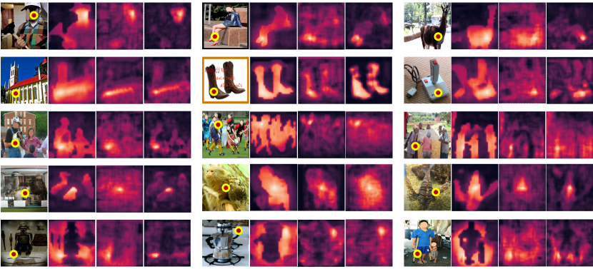
Figure 3: Point affinity visualizations. In total we show 15 groups of examples. In each group from left to right we show the original image with the selected point (denoted by red circle); three affinity maps calculated from the point to the rest of the image with the output of i) our point-level region contrast; ii) region-level contrast; and iii) MoCo v2 (image-level contrast). In rows from top to down, we show 5 categories of picked points: i) single non-rigid objects, ii) single rigid objects, iii) multiple objects, iv) objects in chaotic background and v) background stuff. Brighter colors in the affinity map denote more similar points. Best viewed in color and zoomed in.

Figure 4: Point affinity (failures). We present two kinds of failure cases for our method: under-segmentation (left) and over-segmentation (right). For each kind we show 3 pairs of images, using the same visualization technique in Fig. 3. See text for details.

4.4 Visualization of Point Affinities

In order to provide a more intuitive way to show the effectiveness of our method, we visualize the point affinities after pre-training in Fig. 3.

The images are randomly chosen from the validation set of ImageNet-1K. We follow the previous experimental setting to pre-train 200 epochs on ImageNet-1K. We then resize all image to 896$\times$896, and interpolate the corresponding feature map of Res5 from (28$\times$28) to 56$\times$56 for higher resolution. For each image, we first pick one point (denoted with a red circle), then calculate the point affinity (in terms of cosine similarity) from the last-layer output feature representation of this point to all the others within the same image. In addition, we also compare it with the visualizations from MoCo v2 and a region-level contrast variant of our method to analyse the improvement. The region-level contrast variant is implemented using MoCo v2 framework with grid regions (same as ours), with an AP of 58.2 on VOC. In Fig. 3, from top to down we show 15 different groups of examples which (row-wise) represent 5 categories of picked points: single non-rigid objects, single rigid objects, multiple objects, objects in chaotic background, and background. Within each group, from left to right we show the point affinity of our method, region-level contrast, and the MoCo v2 baseline. Brighter colors on the feature map denote more similar points.

Observations.

For original MoCo, its final global pooling operation intuitively causes a loss in 2D spatial information, since everything is compressed into a single vector for representations. Therefore, when tracing back, the salient regions usually only cover certain closely-connected small area around the picked point. For the region-level contrast baseline, its salient regions can expand to a larger area, but the area is quite blurry and hard to tell the boundaries. For objects (shown in row 1-3), although all three methods show some localization capabilities, ours often predicts sharper and more clear boundaries, indicating a better understanding of the localization of objects. Row 4 shows the objects in chaotic environments, which is hard to recognize even with human eyes. Except for foreground objects, we also test the ability on the background stuff (row 5). It is interesting to see that even for background, ours can still distinguish it with foreground objects.

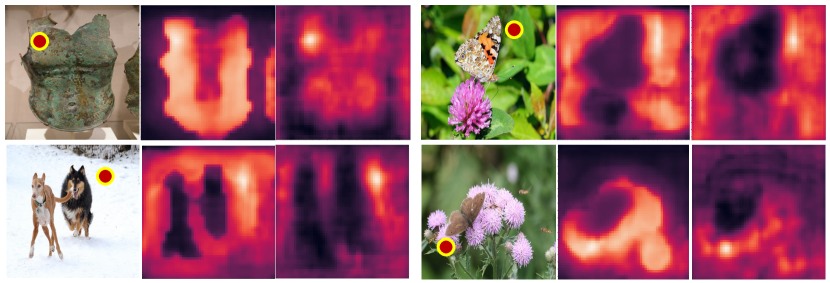
Figure 5: Point affinity with or without affinity distillation. In each of the 4 groups, we show (from left to right) the original image, ours with point affinity distillation and ours without. As can be seen, the distillation loss plays a key role in capturing object boundaries, as shown in the 4 groups of examples.

Failure cases.

We also give some failure cases from our model in Fig. 4. On the left we show under-segmentation, where a segment contains more objects than it should be. For example, in the first image, both the man and the running machine have higher similarity to the chosen point. On the contrary, on the right we show over-segmentation, where a segment does not cover the entire object. For example, the face of the woman has higher similarity to the chosen point, while the clothes and wig have lower similarities – ideally they should all belong to the same person. We believe this is reasonable in our unsupervised setting: without definition of object classes, the model can at best form groups using low-level cues such as textures or colors; therefore, it can miss semantic-level grouping of objects.

random	supervised	image-	region-	ours
15.3	22.9	33.1	33.8	52.0

Table 3: Quantitative metric to compare VOC visualizations from different pre-training methods. Our point-level region contrast outperforms all baselines ranging from random, supervised pre-training and self-supervised pre-training at various levels.

Affinity distillation helps localization.

We visualize our method with or without point affinity distillation in Fig. 5. We find the distillation loss plays a key role in capturing object boundaries for better localization.

Quantitative Metric.

We quantitatively evaluate the visualizations from different pre-training methods on VOC val2007. For each ground-truth object, we pick its center point and calculate the similarity from this point to the rest of the image with the pre-trained model to generate segmentation masks. We pick a threshold to keep 80% of the entire affinity map. The mask is then benchmarked with Jaccard similarity, defined as the intersection over union (IoU) between the predicted mask and the ground-truth one.

Our baselines are: random (no pre-training), supervised (on ImageNet-1K), MoCo v2 (image-level) and region-level. The results are summarized in Tab. 3. As expected, point-level region contrast significantly outperforms others.

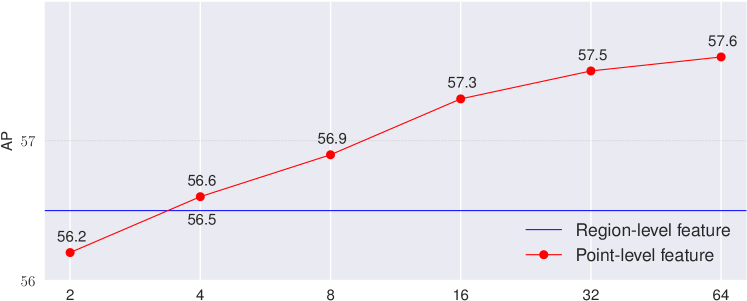
Figure 6: Point-level vs. region-level features. We check how many points are needed to match a region-level representation when pre-trained on ImageNet-1K. Along the horizontal axis the number of points increases from 2 to 64 for point-level features. The pre-trained representation can already match region-level features (blue line) in VOC AP with only 4 points.

4.5 Main Ablation Studies

For our main ablation analysis, we begin with point-level contrastive learning in Sec. 4.5.1, showing its effectiveness to represent regions and robustness to inferior initial regions compared to a region-based counterpart. Then we discuss and compare possible point affinity distillation strategies in Sec. 4.5.2. More ablations are found in the appendix. Throughout this section, we pre-train for 100 epochs on ImageNet-1K and 400 COCO epochs on COCO.

4.5.1 Point-Level vs. Region-Level

We first design experiments to show the motivation and effectiveness of introducing point-level operations to region-level contrast. We conduct two experiments.

First is to see how many points are needed to match the pooled region-level features. We pre-train on ImageNet for 100 epochs without point affinity loss for fair comparisons, and report results with VOC object detection transfer. As shown in Fig. 6, we find with only 4 points per-region, its AP (56.6) is already better than region-level contrast (56.5). Interestingly, more point-level features continue to benefit performance even up to 64 points, which suggests that the pooled, region-level features are not as effective as point-level ones for object detection pre-training.

Second, we add back the point affinity loss and compare the robustness of our full method against contrast learning with aggregated region-level features [23]. For this experiment, we pre-train on COCO as COCO is annotated with ground-truth object boxes/masks. $P{=}$16 points are used per-region and evaluation is also performed with VOC object detection. In Fig. 7 we gradually decrease the region quality, from highest (ground-truth mask), to lowest (2$\times$2 grid) with ground-truth box and 4$\times$4 grid in-between. Not only does point-level region contrast perform better than region-level contrast, the gap between the two increases as the region quality degenerates from left to right. This confirms that our method is more robust to initial region assignments and can work with all types of regions.

4.5.2 Point Affinity Distillation Strategies

For point affinity distillation, there are three possible strategies: 1) ${\bm{A}}_{i^{\prime}k^{\prime}}$ as teacher (see Eq. 3 for its definition), ${\bm{A}}_{ik^{\prime}}$ as student (default); 2) ${\bm{A}}_{ik^{\prime}}$ as teacher, ${\bm{A}}_{ik}$ as student; 3) ${\bm{A}}_{i^{\prime}k^{\prime}}$ as teacher, ${\bm{A}}_{ik}$ as student, which requires an extra forward pass with momentum encoders.

Strategy 1) achieves 58.0 AP. Switching to strategy 2) slightly degenerates AP to 57.6, and strategy 3) yields the same AP as 1) while requiring extra computations. Therefore we set 1) as our default setting.

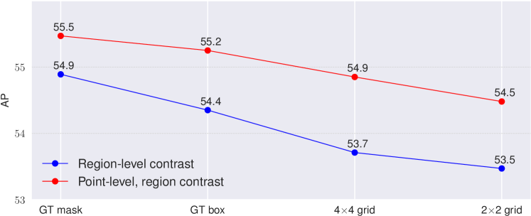
Figure 7: Region quality vs. AP comparison between our point-level region contrast (red) and region-level contrast with pooled-features, pre-trained on COCO. Along the horizontal axis the region quality degenerates: ground truth masks, ground truth bounding box, 4$\times$4 grid and 2$\times$2 grid. Our method is consistently better and is more resilient to the degeneration of region qualities.

5 Conclusion

Balancing recognition and localization, we introduced point-level region contrast, which performs self-supervised pre-training by directly sampling individual point pairs from different regions. Compared to other contrastive formulations, our approach can learn both inter-image and intra-image distinctions, and is more resilient to imperfect unsupervised regions assignments. We empirically verified the effectiveness of our approach on multiple setups and showed strong results against state-of-the-art pre-training methods for object detection. We hope our explorations can provide new perspective and inspirations to the community.

$\alpha$	AP	AP${}_{\text{50}}$	AP${}_{\text{75}}$
0	57.3	82.0	63.8
0.3	57.5	82.1	64.1
0.5	58.0	82.5	64.7
0.7	57.6	82.3	64.3

(a)

$\beta$	AP	AP${}_{\text{50}}$	AP${}_{\text{75}}$
0.3	56.4	81.5	62.4
0.5	57.1	82.1	63.8
0.7	58.0	82.5	64.7
0.9	56.4	81.5	62.5

(b)

$\tau_{s}$	$\tau_{t}$	AP	AP${}_{\text{50}}$	AP${}_{\text{75}}$
0.1	0.04	57.7	82.3	64.4
0.1	0.07	58.0	82.5	64.7
0.2	0.15	57.3	82.1	64.2

(c)

$P$	AP	AP${}_{\text{50}}$	AP${}_{\text{75}}$
8	57.1	81.8	63.9
16	58.0	82.5	64.7
32	58.2	82.7	65.1

(d)

$n$	AP	AP${}_{\text{50}}$	AP${}_{\text{75}}$
2	57.1	82.1	63.7
4	58.0	82.5	64.7
8	57.6	82.2	64.3

(e)

$R$	AP	AP${}_{\text{50}}$	AP${}_{\text{75}}$
14$\times$14	57.3	81.9	63.7
56$\times$56	58.0	82.5	64.7
224$\times$224	57.2	82.2	63.6

(f)

Table 4: Ablation studies. For all of them, we pre-train our representation on ImageNet-1K for 100 epochs, and report the transfer results on VOC object detection. Our default settings are shown in gray.

Acknowledgements.

This work was partially supported by ONR N00014-21-1-2812. We thank the anonymous reviewers for their effort and valuable feedback to improve our work.

Appendix A More Ablation Analysis

Beyond ablation analysis provided in the main paper (Sec. 4.5), we provide three more groups of analysis in this appendix. They are: 1) balance between different losses during pre-training; 2) student and teacher temperatures in point affinity distillation; and 3) hyper-parameters for point sampling. Unless otherwise specified, we use ImageNet-1K and pre-train for 100 epochs. The results are reported on VOC object detection, all summarized in Tab. 4.

A.1 Balance Between Losses

Contrastive & affinity distillation.

The hyper-parameter $\alpha$ in Eq. 5 serves as the weight to balance the two point based loss terms. By default we set $\alpha$ as 0.5 and we report the results of different $\alpha$ values in LABEL:tab:ablation_point_ratio_old.

Image-level & point-level.

On top of point-level computation, we further leverage image-level loss. The hyper-parameter $\beta$ in Eq. 6 serves as the weight to balance the two loss terms. We report the results of different $\beta$ values in LABEL:tab:ablation_image_point_ratio. We find when the image-level loss is small, the overall performance will be influenced, since the point-level task is harder to converge at the beginning. Adding image-level contrastive loss further enhances our method to balance localization and recognition capabilities.

A.2 Temperatures in Point Affinity Distillation

We now study the hyper-parameters for the student and teacher temperatures $\tau_{s}$ and $\tau_{t}$. Intuitively, we hope the output from the teacher is closer to a ‘one-hot’ label [38], which means the teacher temperature is relatively smaller than the student one. We explored a few setups following this intuition, and summarize our observations in LABEL:tab:temperature.

From the default temperatures, our method is quite robust to the changes. For example, decreasing $\tau_{t}$ from 0.07 to 0.04 only slightly degenerates the performance. Varying both temperatures also do not affect much in the third row.

A.3 Point Sampling

Number of points $P$.

For final loss which includes the point affinity, we also ablate the number of points. From the results in LABEL:tab:ablation_point_number we can observe the performance improves as the point number increases. We use point number $P{=}$16 as the default setting, where the performance starts to saturate. We report the results of different number of points.

Number of grids $n$.

In the default setting, the adopted grid number is 4$\times$4. We report the results of different number of grids in LABEL:tab:ablation_grid_number. From the table, we observe the number of grid does not influence the results much.

Feature map resolution $R$.

In the default setting, we up-sample the feature map to 56$\times$56. From LABEL:tab:ablation_resolution, we can observe that feature map resolution would also influence the results, with 56 x 56 further directing towards better AP.

Appendix B More Visualizations

We provide more visualizations with our method in Fig. 8. We followed the same protocol which first pick a point (denoted by red circle), and then compute the affinity map with the pre-trained features. Brighter colors denote more similar points. Our method consistently generates masks with crisp boundaries.

Appendix C License of Assets

Dataset	Licence
ImageNet	https://image-net.org/download.php
COCO	Creative Commons Attribution 4.0 License
Pascal VOC	http://host.robots.ox.ac.uk/pascal/VOC/
Cityscapes	https://www.cityscapes-dataset.com/license/

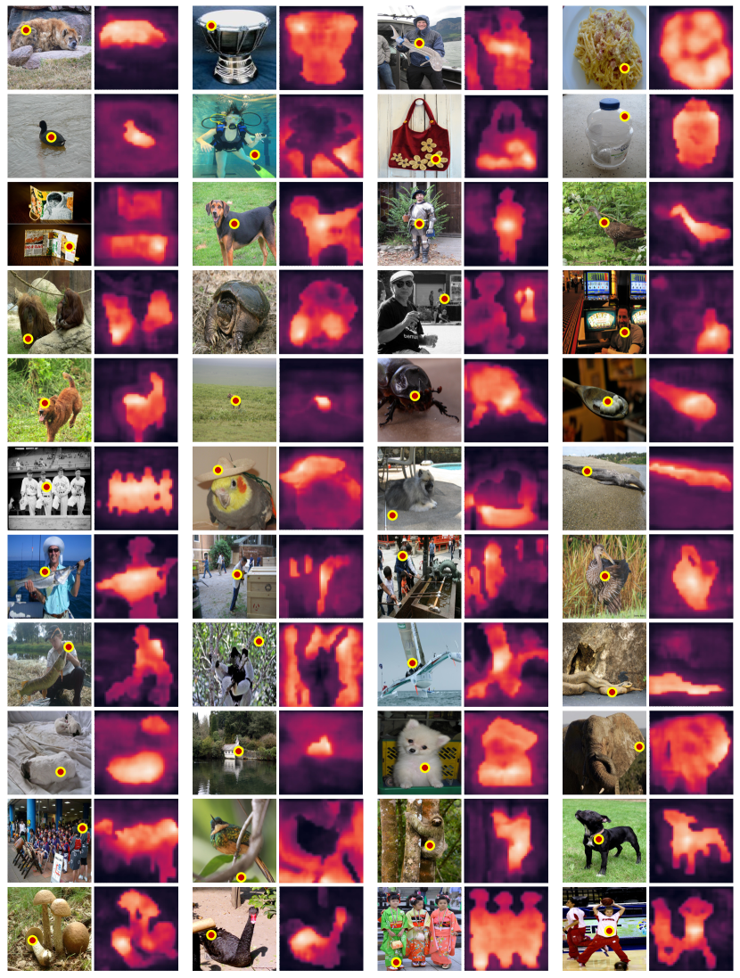
Figure 8: More visualizations on ImageNet-1K with our point-level region contrast.

References

- [1] Lvis challenge 2021. https://www.lvisdataset.org/challenge_2021. Accessed: 2021-11-16.
- [2] Pablo Arbeláez, Jordi Pont-Tuset, Jonathan T Barron, Ferran Marques, and Jitendra Malik. Multiscale combinatorial grouping. In CVPR, 2014.
- [3] Tom Brown, Benjamin Mann, Nick Ryder, Melanie Subbiah, Jared D Kaplan, Prafulla Dhariwal, Arvind Neelakantan, Pranav Shyam, Girish Sastry, Amanda Askell, Sandhini Agarwal, Ariel Herbert-Voss, Gretchen Krueger, Tom Henighan, Rewon Child, Aditya Ramesh, Daniel Ziegler, Jeffrey Wu, Clemens Winter, Chris Hesse, Mark Chen, Eric Sigler, Mateusz Litwin, Scott Gray, Benjamin Chess, Jack Clark, Christopher Berner, Sam McCandlish, Alec Radford, Ilya Sutskever, and Dario Amodei. Language models are few-shot learners. In NeurIPS, 2020.
- [4] Mathilde Caron, Hugo Touvron, Ishan Misra, Hervé Jégou, Julien Mairal, Piotr Bojanowski, and Armand Joulin. Emerging properties in self-supervised vision transformers. In ICCV, 2021.
- [5] Neelima Chavali, Harsh Agrawal, Aroma Mahendru, and Dhruv Batra. Object-proposal evaluation protocol is ‘gameable’. In CVPR, 2016.
- [6] Ting Chen, Simon Kornblith, Mohammad Norouzi, and Geoffrey Hinton. A simple framework for contrastive learning of visual representations. In ICML, 2020.
- [7] Xinlei Chen, Haoqi Fan, Ross Girshick, and Kaiming He. Improved baselines with momentum contrastive learning. arXiv preprint arXiv:2003.04297, 2020.
- [8] Xinlei Chen and Kaiming He. Exploring simple siamese representation learning. In CVPR, 2021.
- [9] Bowen Cheng, Omkar Parkhi, and Alexander Kirillov. Pointly-supervised instance segmentation. arXiv preprint arXiv:2104.06404, 2021.
- [10] Marius Cordts, Mohamed Omran, Sebastian Ramos, Timo Rehfeld, Markus Enzweiler, Rodrigo Benenson, Uwe Franke, Stefan Roth, and Bernt Schiele. The cityscapes dataset for semantic urban scene understanding. In CVPR, pages 3213–3223, 2016.
- [11] Marco Cuturi. Sinkhorn distances: Lightspeed computation of optimal transport. NeurIPS, 2013.
- [12] Jia Deng, Wei Dong, Richard Socher, Li-Jia Li, Kai Li, and Li Fei-Fei. ImageNet: A large-scale hierarchical image database. In CVPR, 2009.
- [13] Jacob Devlin, Ming-Wei Chang, Kenton Lee, and Kristina Toutanova. BERT: pre-training of deep bidirectional transformers for language understanding. CoRR, abs/1810.04805, 2018.
- [14] Alexey Dosovitskiy, Jost Tobias Springenberg, Martin Riedmiller, and Thomas Brox. Discriminative unsupervised feature learning with convolutional neural networks. In NeurIPS, 2014.
- [15] Debidatta Dwibedi, Yusuf Aytar, Jonathan Tompson, Pierre Sermanet, and Andrew Zisserman. With a little help from my friends: Nearest-neighbor contrastive learning of visual representations. arXiv preprint arXiv:2104.14548, 2021.
- [16] Mark Everingham, Luc Van Gool, Christopher KI Williams, John Winn, and Andrew Zisserman. The PASCAL Visual Object Classes (VOC) Challenge. IJCV, 88(2):303–338, 2010.
- [17] Golnaz Ghiasi, Yin Cui, Aravind Srinivas, Rui Qian, Tsung-Yi Lin, Ekin D Cubuk, Quoc V Le, and Barret Zoph. Simple copy-paste is a strong data augmentation method for instance segmentation. In CVPR, 2021.
- [18] Ross Girshick, Jeff Donahue, Trevor Darrell, and Jitendra Malik. Rich feature hierarchies for accurate object detection and semantic segmentation. In CVPR, 2014.
- [19] Jean-Bastien Grill, Florian Strub, Florent Altché, Corentin Tallec, Pierre Richemond, Elena Buchatskaya, Carl Doersch, Bernardo Avila Pires, Zhaohan Guo, Mohammad Gheshlaghi Azar, et al. Bootstrap your own latent-a new approach to self-supervised learning. NeurIPS, 2020.
- [20] Kaiming He, Haoqi Fan, Yuxin Wu, Saining Xie, and Ross Girshick. Momentum contrast for unsupervised visual representation learning. In CVPR, 2020.
- [21] Kaiming He, Georgia Gkioxari, Piotr Dollár, and Ross Girshick. Mask R-CNN. In ICCV, 2017.
- [22] Kaiming He, Xiangyu Zhang, Shaoqing Ren, and Jian Sun. Deep residual learning for image recognition. In CVPR, 2016.
- [23] Olivier J Hénaff, Skanda Koppula, Jean-Baptiste Alayrac, Aaron van den Oord, Oriol Vinyals, and João Carreira. Efficient visual pretraining with contrastive detection. In ICCV, 2021.
- [24] Olivier J Hénaff, Aravind Srinivas, Jeffrey De Fauw, Ali Razavi, Carl Doersch, SM Eslami, and Aaron van den Oord. Data-efficient image recognition with contrastive predictive coding. arXiv preprint arXiv:1905.09272, 2019.
- [25] Geoffrey Hinton, Oriol Vinyals, and Jeff Dean. Distilling the knowledge in a neural network. arXiv preprint arXiv:1503.02531, 2015.
- [26] Alexander Kirillov, Yuxin Wu, Kaiming He, and Ross Girshick. Pointrend: Image segmentation as rendering. In CVPR, 2020.
- [27] Tsung-Yi Lin, Priya Goyal, Ross Girshick, Kaiming He, and Piotr Dollár. Focal loss for dense object detection. In ICCV, 2017.
- [28] Tsung-Yi Lin, Michael Maire, Serge Belongie, James Hays, Pietro Perona, Deva Ramanan, Piotr Dollár, and Lawrence Zitnick. Microsoft COCO: Common objects in context. In ECCV, 2014.
- [29] Songtao Liu, Zeming Li, and Jian Sun. Self-emd: Self-supervised object detection without imagenet. arXiv preprint arXiv:2011.13677, 2020.
- [30] Wei Liu, Dragomir Anguelov, Dumitru Erhan, Christian Szegedy, Scott Reed, Cheng-Yang Fu, and Alexander C Berg. Ssd: Single shot multibox detector. In ECCV, 2016.
- [31] Jonathan Long, Evan Shelhamer, and Trevor Darrell. Fully convolutional networks for semantic segmentation. In CVPR, 2015.
- [32] Jitendra Malik, Pablo Arbeláez, João Carreira, Katerina Fragkiadaki, Ross Girshick, Georgia Gkioxari, Saurabh Gupta, Bharath Hariharan, Abhishek Kar, and Shubham Tulsiani. The three r’s of computer vision: Recognition, reconstruction and reorganization. Pattern Recognition Letters, 72:4–14, 2016.
- [33] Pedro O Pinheiro, Amjad Almahairi, Ryan Y Benmaleck, Florian Golemo, and Aaron Courville. Unsupervised learning of dense visual representations. arXiv preprint arXiv:2011.05499, 2020.
- [34] Alec Radford, Jeffrey Wu, Rewon Child, David Luan, Dario Amodei, Ilya Sutskever, et al. Language models are unsupervised multitask learners. OpenAI blog, 1(8):9, 2019.
- [35] Shaoqing Ren, Kaiming He, Ross Girshick, and Jian Sun. Faster r-cnn: Towards real-time object detection with region proposal networks. In NeurIPS, 2015.
- [36] Byungseok Roh, Wuhyun Shin, Ildoo Kim, and Sungwoong Kim. Spatially consistent representation learning. In CVPR, 2021.
- [37] Olga Russakovsky, Jia Deng, Hao Su, Jonathan Krause, Sanjeev Satheesh, Sean Ma, Zhiheng Huang, Andrej Karpathy, Aditya Khosla, Michael Bernstein, et al. Imagenet large scale visual recognition challenge. IJCV, 115(3):211–252, 2015.
- [38] Kihyuk Sohn, David Berthelot, Chun-Liang Li, Zizhao Zhang, Nicholas Carlini, Ekin D Cubuk, Alex Kurakin, Han Zhang, and Colin Raffel. Fixmatch: Simplifying semi-supervised learning with consistency and confidence. arXiv preprint arXiv:2001.07685, 2020.
- [39] Yonglong Tian, Dilip Krishnan, and Phillip Isola. Contrastive multiview coding. arXiv preprint arXiv:1906.05849, 2019.
- [40] Yonglong Tian, Chen Sun, Ben Poole, Dilip Krishnan, Cordelia Schmid, and Phillip Isola. What makes for good views for contrastive learning. In NeurIPS, 2020.
- [41] Jasper RR Uijlings, Koen EA Van De Sande, Theo Gevers, and Arnold WM Smeulders. Selective search for object recognition. IJCV, 104(2):154–171, 2013.
- [42] Aaron van den Oord, Yazhe Li, and Oriol Vinyals. Representation learning with contrastive predictive coding. arXiv preprint arXiv:1807.03748, 2018.
- [43] Xinlong Wang, Rufeng Zhang, Chunhua Shen, Tao Kong, and Lei Li. Dense contrastive learning for self-supervised visual pre-training. arXiv preprint arXiv:2011.09157, 2020.
- [44] Fangyun Wei, Yue Gao, Zhirong Wu, Han Hu, and Stephen Lin. Aligning pretraining for detection via object-level contrastive learning. NeurIPS, 2021.
- [45] Yuxin Wu, Alexander Kirillov, Francisco Massa, Wan-Yen Lo, and Ross Girshick. Detectron2. https://github.com/facebookresearch/detectron2, 2019.
- [46] Zhirong Wu, Yuanjun Xiong, Stella Yu, and Dahua Lin. Unsupervised feature learning via non-parametric instance discrimination. In CVPR, 2018.
- [47] Tete Xiao, Colorado J Reed, Xiaolong Wang, Kurt Keutzer, and Trevor Darrell. Region similarity representation learning. In ICCV, 2021.
- [48] Enze Xie, Jian Ding, Wenhai Wang, Xiaohang Zhan, Hang Xu, Peize Sun, Zhenguo Li, and Ping Luo. Detco: Unsupervised contrastive learning for object detection. In CVPR, 2021.
- [49] Jiahao Xie, Xiaohang Zhan, Ziwei Liu, Yew Ong, and Chen Change Loy. Unsupervised object-level representation learning from scene images. Advances in Neural Information Processing Systems, 34, 2021.
- [50] Saining Xie, Jiatao Gu, Demi Guo, Charles R Qi, Leonidas Guibas, and Or Litany. Pointcontrast: Unsupervised pre-training for 3d point cloud understanding. In ECCV, 2020.
- [51] Zhenda Xie, Yutong Lin, Zheng Zhang, Yue Cao, Stephen Lin, and Han Hu. Propagate yourself: Exploring pixel-level consistency for unsupervised visual representation learning. In CVPR, 2021.
- [52] Ceyuan Yang, Zhirong Wu, Bolei Zhou, and Stephen Lin. Instance localization for self-supervised detection pretraining. In CVPR, 2021.
- [53] Xiao Zhang and Michael Maire. Self-supervised visual representation learning from hierarchical grouping. arXiv preprint arXiv:2012.03044, 2020.
- [54] C Lawrence Zitnick and Piotr Dollár. Edge boxes: Locating object proposals from edges. In ECCV, 2014.