A Local Geometric Interpretation of Feature Extraction in Deep Feedforward Neural Networks

Abstract

In this paper, we present a local geometric analysis to interpret how deep feedforward neural networks extract low-dimensional features from high-dimensional data. Our study shows that, in a local geometric region, the optimal weight in one layer of the neural network and the optimal feature generated by the previous layer comprise a low-rank approximation of a matrix that is determined by the Bayes action of this layer. This result holds (i) for analyzing both the output layer and the hidden layers of the neural network, and (ii) for neuron activation functions with non-vanishing gradients. We use two supervised learning problems to illustrate our results: neural network based maximum likelihood classification (i.e., softmax regression) and neural network based minimum mean square estimation. Experimental validation of these theoretical results will be conducted in our future work.

I introduction

In recent years, neural network based supervised learning has been extensively admired due to its emerging applications in a wide range of inference problems, such as image classification, DNA sequencing, natural language processing, etc. The success of deep neural networks depends heavily on its capability of extracting good low-dimensional features from high-dimensional data. Due to the complexity of deep neural networks, theoretical interpretation of feature extraction in deep neural networks has been challenging, with some recent progress reported in, e.g., [1, 2, 3, 4, 5, 6, 7, 8, 9, 10, 11, 12, 13].

In this paper, we analyze the training of deep feedforward neural networks for a class of empirical risk minimization (ERM) based supervised learning algorithms. A local geometric analysis is conducted for feature extraction in deep feedforward neural networks. Specifically, the technical contributions of this paper are summarized as follows:

• We first analyze the design of (i) the weights and biases in the output layer and (ii) the feature constructed by the last hidden layer. In a local geometric region, this design problem is converted to a low-rank matrix approximation problem, where the matrix is characterized by the Bayes action of the supervised learning problem. Optimal designs of the weights, biases, and feature are derived in the local geometric region (see Theorems 1-3).

• The above local geometric analysis can be readily applied to a hidden layer (see Corollaries 2-4), by considering another supervised learning problem for the hidden layer. The local geometric analyses of different layers are related to each other in an iterative manner: The optimal feature obtained from the analysis of one layer is the Bayes action needed for analyzing the previous layer. We use two supervised learning problems to illustrate our results.

I-A Related Work

Due to the practical success of deep neural networks, there have been numerous efforts [1, 2, 3, 4, 5, 6, 7, 8, 9, 10, 11, 12, 13] to explain the feature extraction procedure of deep neural networks. Towards this end, researchers have used different approaches, for example, statistical learning theory approach [1, 2], information geometric approach [3, 4, 5, 6, 7, 8, 9, 10], information theoretic approach [10, 11, 12], etc. The information bottleneck formulation in [11] suggested that the role of the deep neural network is to learn minimal sufficient statistics of the data for an inference task. The authors in [12] proposed that maximal coding rate reduction is a fundamental principle in deep neural networks. In [10], the authors formulated the problem of feature extraction by using KL-divergence, and provided a local geometric analysis by considering a weak dependency between the data and the label. Motivated by [10], we also consider the weak dependency. Compared to [10], our local geometric analysis can handle more general supervised learning problems and neuron activation functions, as explained in Section III.

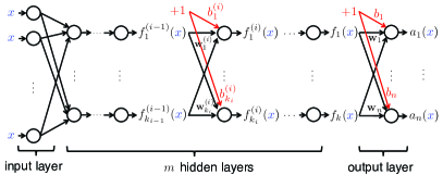
Figure 1: A deep feedforward neural network.

II Model and Problem

II-A Deep Feedforward Neural Network Model

Consider the deep feedforward neural network illustrated in Figure 1, which consists of one input layer, $m$ hidden layers, and one output layer. The input layer admits an input variable $x\in\mathcal{X}$ and feeds a vector

$$\mathbf{f}^{(0)}(x)=[h^{(0)}_{1}(x),\ldots,h_{k_{0}}^{(0)}(x)]^{\operatorname{T}}\in\mathbb{R}^{k_{0}}$$ (1)

to the first hidden layer, where $k_{0}$ is the number of neurons in the input layer and $h^{(0)}_{j}:\mathcal{X}\mapsto\mathbb{R}$ is the activation function of the $j$-th neuron in the input layer. For all $i=1,\ldots,m$, the $i$-th hidden layer admits $\mathbf{f}^{(i-1)}(x)\in\mathbb{R}^{k_{i-1}}$ from the previous layer and constructs a vector $\mathbf{f}^{(i)}(x)\in\mathbb{R}^{k_{i}}$, usually called a feature, given by

$$\mathbf{f}^{(i)}(x)$$

$$= \!\left[h^{\!(i)}\!(\mathbf{w}_{1}^{(i)\!\operatorname{T}}\mathbf{f}^{(i-1)}\!(x)\!+\!b^{(i)}_{1}),\ldots,h^{\!(i)}\!(\mathbf{w}_{k_{i}}^{(i)\!\operatorname{T}}\mathbf{f}^{(i-1)}\!(x)\!+\!b^{(i)}_{k_{i}})\right]^{\operatorname{T}}\!\!,$$ (2)

where $k_{i}$ is the number of neurons in the $i$-th hidden layer, $h^{(i)}:\mathbb{R}\mapsto\mathbb{R}$ is the activation function of each neuron in the $i$-th hidden layer, $\mathbf{w}_{j}^{(i)}\in\mathbb{R}^{k_{i-1}}$ and $b_{j}^{(i)}\in\mathbb{R}$ are the weight vector and bias of the $j$-th neuron in the $i$-th hidden layer, respectively. Denote $\mathbf{W}^{(i)}=[\mathbf{w}^{(i)}_{1},\ldots,\mathbf{w}^{(i)}_{k_{i}}]$ and $\mathbf{b}^{(i)}=$ $[b^{(i)}_{1},\ldots,b^{(i)}_{k_{i}}]^{\operatorname{T}}$, then (II-A) can be expressed compactly as

$$\mathbf{f}^{(i)}(x)=\mathbf{h}^{(i)}\left(\mathbf{W}^{(i)\operatorname{T}}\mathbf{f}^{(i-1)}(x)+\mathbf{b}^{(i)}\right),$$ (3)

where $\mathbf{h}^{(i)}:\mathbb{R}^{k_{i}}\mapsto\mathbb{R}^{k_{i}}$ is a vector-valued function determined by (II-A). For notational simplicity, let us denote $k=k_{m}$ and $\mathbf{f}(x)=\mathbf{f}^{(m)}(x)$. The output layer admits $\mathbf{f}(x)\in\mathbb{R}^{k}$ from the last hidden layer and generates an output vector $\mathbf{a}(x)\in\mathcal{H}^{n}$, called an action, which is determined by

$$\mathbf{a}(x)= {\mathbf{h}}(\mathbf{W}^{\operatorname{T}}\mathbf{f}(x)+\mathbf{b})$$

$$= [h(\mathbf{w}_{1}^{\operatorname{T}}\mathbf{f}(x)+b_{1}),\cdots,h(\mathbf{w}_{n}^{\operatorname{T}}\mathbf{f}(x)+b_{n})]^{\operatorname{T}},$$ (4)

where $n$ is the number of neurons in the output layer, $h:\mathbb{R}\mapsto\mathcal{H}$ is the activation function of each neuron in the output layer, $\mathcal{H}$ is the image set of $h$ with $\mathcal{H}\subseteq\mathbb{R}$, $\mathbf{w}_{j}\in\mathbb{R}^{k}$ and $b_{j}\in\mathbb{R}$ are the weight vector and bias of the $j$-th neuron in the output layer, respectively, $\mathbf{W}=[\mathbf{w}_{1},\ldots,\mathbf{w}_{n}]$ and $\mathbf{b}=[b_{1},\ldots,b_{n}]^{\operatorname{T}}$.

II-B Neural Network based Supervised Learning Problem

The above deep feedforward neural network is used to solve a supervised learning problem. We focus on a class of popular supervised learning algorithms called empirical risk minimization (ERM). In ERM algorithms, the weights and biases of the neural network are trained to construct a vector-valued function $\mathbf{a}:\mathcal{X}\mapsto\mathcal{A}$ that outputs an action $\mathbf{a}(x)\in\mathcal{A}$ for each $x\in\mathcal{X}$, where $\mathcal{A}\subseteq\mathcal{H}^{n}\subseteq\mathbb{R}^{n}$. Consider two random variables $X\in\mathcal{X}$ and $Y\in\mathcal{Y}$, where $\mathcal{X}$ and $\mathcal{Y}$ are finite sets. The performance of an ERM algorithm is measured by a loss function $L:\mathcal{Y}\times\mathcal{A}\mapsto\mathbb{R}$, where $L(y,\mathbf{a}(x))$ is the incurred loss if action $\mathbf{a}(x)$ is generated by the neural network when $Y=y$. For example, in neural network based maximum likelihood classification, also known as softmax regression, the loss function is

$$L_{\log}(y,\mathbf{a})=-\log\left(\frac{a_{y}}{\sum_{y^{\prime}\in\mathcal{Y}}a_{y^{\prime}}}\right),$$ (5)

which is the negative log-likelihood of a distribution $Q_{Y}$ generated by the neural network, where $Q_{Y}(y)={a_{y}}/{\sum_{y^{\prime}\in\mathcal{Y}}a_{y^{\prime}}}$, $a_{y}>0$ for all $y\in\mathcal{Y}$, and the dimension of $\mathbf{a}$ is $n=|\mathcal{Y}|$. In neural network based minimum mean-square estimation, the loss function is one half of the mean-square error between $\mathbf{y}\in\mathbb{R}^{n}$ and an estimate $\hat{\mathbf{y}}=\mathbf{a}(x)\in\mathbb{R}^{n}$ constructed by the neural network, i.e.,

$$L_{2}(\mathbf{y},\hat{\mathbf{y}})=\frac{1}{2}\|\mathbf{y}-\hat{\mathbf{y}}\|_{2}^{2}.$$ (6)

Let $P_{X,Y}$ be the empirical joint distribution of $X$ and $Y$ in the training data, $P_{X}$ and $P_{Y}$ be the associated marginal distributions, which satisfies $P_{X}(x)>0$ for all $x\in\mathcal{X}$ and $P_{Y}(y)>0$ for all $y\in\mathcal{Y}$. The objective of ERM algorithms is to solve the following neural network training problem:

$$\min_{\begin{subarray}{c}(\mathbf{W},\mathbf{b}),\\ ~{}(\mathbf{W}^{(i)},\mathbf{b}^{(i)}),i=1,\ldots,m\end{subarray}}\mathbb{E}_{X,Y\sim P_{X,Y}}[L\left(Y,\mathbf{a}(X)\right)],$$ (7)

where $\mathbf{a}(x)$ is subject to (1)-(II-A), because $\mathbf{a}(x)$ is the action generated by the neural network.

II-C Problem Reformulation

Denote $\Phi=\{f:\mathcal{X}\mapsto\mathcal{A}\}$ as the set of all functions from $\mathcal{X}$ to $\mathcal{A}$. Any action function $\mathbf{a}(x)$ produced by the neural network, i.e., any function satisfying (1)-(II-A), belongs to $\Phi$, whereas some functions in $\Phi$ cannot be constructed by the neural network. By relaxing the set of feasible action functions in (7) as $\Phi$, we derive the following lower bound of (7):

$$\min_{\mathbf{a}\in\Phi}\mathbb{E}_{X,Y\sim P_{X,Y}}[L(Y,\mathbf{a}(X))]$$ (8)

$$= \sum_{x\in\mathcal{X}}P_{X}(x)\min_{\mathbf{a}(x)\in\mathcal{A}}\mathbb{E}_{Y\sim P_{Y|X=x}}[L(Y,\mathbf{a}(x))],$$ (9)

where (8) is decomposed into a sequence of separable optimization problems in (9), each optimizing the action $\mathbf{a}(x)\in\mathcal{A}$ for a given $x\in\mathcal{X}$. Let $\mathcal{A}_{P_{Y}}\subseteq\mathcal{A}$ denote the set of optimal solutions to the following problem:

$$\mathcal{A}_{P_{Y}}=\arg\min_{\mathbf{a}\in\mathcal{A}}\mathbb{E}_{Y\sim P_{Y}}[L(Y,\mathbf{a})]$$ (10)

and use $\mathbf{a}_{P_{Y}}$ to denote an element of $\mathcal{A}_{P_{Y}}$, which is usually called a Bayes action. Define the discrepancy

$$D_{L}(\mathbf{a}_{P_{Y}}||\mathbf{a})=\mathbb{E}_{Y\sim P_{Y}}[L(Y,\mathbf{a})]-\mathbb{E}_{Y\sim P_{Y}}[L(Y,\mathbf{a}_{P_{Y}})].$$ (11)

According to (10) and (11), $D_{L}(\mathbf{a}_{P_{Y}}||\mathbf{a})\geq 0$ for all $\mathbf{a}\in\mathcal{A}$, where equality is achieved if and only if $\mathbf{a}\in\mathcal{A}_{P_{Y}}$. When $\mathbf{a}=\mathbf{a}_{Q_{Y}}$, $D_{L}(\mathbf{a}_{P_{Y}}||\mathbf{a}_{Q_{Y}})$ is a generalized divergence between $P_{Y}$ and $Q_{Y}$ [14, 15].

By subtracting the lower bound (9) from (7), we obtain the following problem that is equivalent to (7):

$$\min_{\begin{subarray}{c}(\mathbf{W},\mathbf{b}),\\ ~{}(\mathbf{W}^{(i)},\mathbf{b}^{(i)}),i=1,\ldots,m\end{subarray}}\sum_{x\in\mathcal{X}}P_{X}(x)D_{L}(\mathbf{a}_{P_{Y|X=x}}||\mathbf{a}(x)),$$ (12)

where $\mathbf{a}_{P_{Y|X=x}}\in\mathcal{A}_{P_{Y|X=x}}$ is a Bayes action associated with the conditional empirical distribution $P_{Y|X=x}$ and $\mathbf{a}(x)$ is subject to (1)-(II-A).

III Main Results: Feature Extraction in
Deep Feedforward Neural Networks

III-A Local Geometric Analysis of the Output Layer

We consider the following reformulation of (12) that focuses on the training of the output layer:

$$\min_{\begin{subarray}{c}\mathbf{W}\in\mathbb{R}^{k\times n},\\ \mathbf{b}\in\mathbb{R}^{n},\mathbf{f}\in\Lambda\end{subarray}}~{}\sum_{x\in\mathcal{X}}P_{X}(x)D_{L}(\mathbf{a}_{P_{Y|X=x}}||\mathbf{h}(\mathbf{W}^{\operatorname{T}}\mathbf{f}(x)+\mathbf{b})),$$ (13)

where $\Lambda$ is the set of feature functions created by the input and hidden layers of the neural network.

Recall that $\mathcal{H}^{n}$ is the image set of the vector-valued activation function $\mathbf{h}(\mathbf{b})$ of the output layer. Because $\mathcal{A}_{P_{Y}}\subseteq\mathcal{A}\subseteq\mathcal{H}^{n}$, for any Bayes action $\mathbf{a}_{P_{Y}}\in\mathcal{A}_{P_{Y}}$ that solves (10), there exists a bias $\tilde{\mathbf{b}}=[\tilde{b}_{1},\ldots,\tilde{b}_{n}]^{\operatorname{T}}\in\mathbb{R}^{n}$ such that

$$\mathbf{h}(\tilde{\mathbf{b}})=[h(\tilde{b}_{1}),\ldots,h(\tilde{b}_{n})]^{\operatorname{T}}=\mathbf{a}_{P_{Y}}.$$ (14)

The following assumption is needed in our study.

Assumption 1.

For each $i=1,\ldots,n$, there exist $\delta>0$ and $K>0$ such that for all $z\in(\tilde{b}_{i}-\delta,\tilde{b}_{i}+\delta)$, the activation function $h$ satisfies

$$\left|h(z)-h(\tilde{b}_{i})\right|\geq K\left|z-\tilde{b}_{i}\right|.$$ (15)

Lemma 1.

If $h$ is strictly increasing and continuously differentiable, then $h$ satisfies Assumption 1.

Proof.

See Appendix A. ∎

It is easy to see that the leaky ReLU activation function [16, pp. 187-188] satisfies Assumption 1. In addition, the hyperbolic tangent function and the sigmoid function [16, p. 189] also satisfy Assumption 1, because they are strictly increasing and continuously differentiable.

Let $\mathcal{P}^{\mathcal{Y}}$ be the set of all probability distributions on $\mathcal{Y}$ and $\text{relint}(\mathcal{P}^{\mathcal{Y}})$ be the relative interior of the set $\mathcal{P}^{\mathcal{Y}}$.

Assumption 2.

If two distributions $P_{Y},Q_{Y}\in\text{{relint}}(\mathcal{P}^{\mathcal{Y}})$ are close to each other such that

$$\sum_{y\in\mathcal{Y}}(P_{Y}(y)-Q_{Y}(y))^{2}\leq\gamma^{2},$$ (16)

then for any $\mathbf{a}_{P_{Y}}\in\mathcal{A}_{P_{Y}}$, there exists an $\mathbf{a}_{Q_{Y}}\in\mathcal{A}_{Q_{Y}}$ such that

$$\|\mathbf{a}_{P_{Y}}-\mathbf{a}_{Q_{Y}}\|_{2}=O(\gamma).$$ (17)

Assumption 2 characterizes the differentiability of the Bayes action $\mathbf{a}_{P_{Y}}$ with respect to $P_{Y}$. The loss functions in (5) and (6) satisfy Assumption 2, as explained later in Section III-C.

Because of the universal function approximation properties of deep feedforward neural networks [17, 18, 16], we make the following assumption.

Assumption 3.

For given $\epsilon>0$ and $\mathbf{a}_{P_{Y|X=x}}\in\mathcal{A}_{P_{Y|X=x}}$ with $x\in\mathcal{X}$, there exists an optimal solution $(\mathbf{f},\mathbf{W},\mathbf{b})$ to (13) such that for all $x\in\mathcal{X}$

$$\|\mathbf{a}_{P_{Y|X=x}}-\mathbf{h}({\mathbf{W}}^{\operatorname{T}}{\mathbf{f}}(x)+{\mathbf{b}})\|_{2}^{2}\leq\epsilon^{2}.$$ (18)

By Assumption 3, the neural network can closely approximate the vector-valued function $x\mapsto\mathbf{a}_{P_{Y|X=x}}$.

Definition 1.

For a given $\epsilon>0$, two random variables $X$ and $Y$ are called $\epsilon$-dependent, if the $\chi^{2}$-mutual information $I_{\chi^{2}}(X;Y)$ is no more than $\epsilon^{2}$, given by

$$I_{\chi^{2}}(X;Y)=D_{\chi^{2}}(P_{X,Y}||P_{X}\otimes P_{Y})\leq\epsilon^{2},$$ (19)

where

$$D_{\chi^{2}}(P_{X}||Q_{X})=\int_{\mathcal{X}}\frac{(P(x)-Q(x))^{2}}{Q^{2}(x)}dQ(x)$$ (20)

is Neyman’s $\chi^{2}$-divergence [19].

Motivated by the seminal work [10] and [20], we consider the following assumption.

Assumption 4.

For a given $\epsilon>0$, $X$ and $Y$ are $\epsilon$-dependent.

By using the above assumptions, we can find a local geometric region (21) that is useful for our analysis.

Lemma 2.

For a sufficiently small $\epsilon>0$, if Assumptions 1-4 hold, then there exists an optimal solution $(\mathbf{f},\mathbf{W},\mathbf{b})$ to (13) such that for all $x\in\mathcal{X}$ and $i=1,\ldots,n$

$${\mathbf{w}_{i}}^{\operatorname{T}}\mathbf{f}(x)+b_{i}-\tilde{b}_{i}=O(\epsilon).$$ (21)

Proof.

See Appendix B. ∎

For any feature $\mathbf{f}(x)\in\mathbb{R}^{k}$, define a matrix $\mathbf{\Xi}_{\mathbf{f}}\in\mathbb{R}^{k\times|\mathcal{X}|}$ as

$$\mathbf{\Xi}_{\mathbf{f}}=[\bm{\xi}_{\mathbf{f}}(1),\ldots,\bm{\xi}_{\mathbf{f}}(|\mathcal{X}|)],$$ (22)

where

$$\bm{\xi}_{\mathbf{f}}(x)= \sqrt{P_{X}(x)}\left(\mathbf{f}(x)-\bm{\mu}_{\mathbf{f}}\right),$$ (23)

$$\bm{\mu}_{\mathbf{f}}= \sum_{x\in\mathcal{X}}P_{X}(x)\mathbf{f}(x).$$ (24)

In addition, define the following matrix $\mathbf{B}\in\mathbb{R}^{n\times|\mathcal{X}|}$ based on the Bayes actions $\mathbf{a}_{P_{Y|X=x}}$ for $x\in\mathcal{X}$:

$$\mathbf{B}=[\bm{\beta}_{Y}(1),\ldots,\bm{\beta}_{Y}(|\mathcal{X}|)],$$ (25)

where

$$\bm{\beta}_{Y}(x)= \sqrt{P_{X}(x)}\left(\mathbf{a}_{P_{Y|X=x}}-\bm{\mu}_{\mathbf{a}}\right),$$ (26)

$$\bm{\mu}_{\mathbf{a}}= \sum_{x\in\mathcal{X}}P_{X}(x)\mathbf{a}_{P_{Y|X=x}}.$$ (27)

Assumption 5.

The function $\mathbf{a}\mapsto L(y,\mathbf{a})$ is twice continuously differentiable.

The Hessian matrix $\mathbf{M}_{L}$ of the function $\mathbf{a}\mapsto\mathbb{E}_{Y\sim P_{Y}}[L(Y,\mathbf{a})]$ at the point $\mathbf{a}=\mathbf{a}_{P_{Y}}$ is

$$\mathbf{M}_{L}=\frac{\partial^{2}\mathbb{E}_{Y\sim P_{Y}}[L(Y,\mathbf{a})]}{\partial\mathbf{a}\partial\mathbf{a}^{\operatorname{T}}}\bigg{|}_{\mathbf{a}=\mathbf{a}_{P_{Y}}}.$$ (28)

Because $\mathbf{a}_{P_{Y}}$ is an optimal solution to (10), $\mathbf{M}_{L}$ is positive semi-definite. Hence, it has a Cholesky decomposition $\mathbf{M}_{L}=\mathbf{R}_{L}^{\operatorname{T}}\mathbf{R}_{L}.$ The Jacobian matrix of $\mathbf{h}(\mathbf{b})$ at the point $\mathbf{b}=\tilde{\mathbf{b}}$ is

$$\mathbf{J}=\frac{\partial\mathbf{h}(\mathbf{b})}{\partial\mathbf{b}^{\operatorname{T}}}\bigg{|}_{\mathbf{b}=\tilde{\mathbf{b}}}.$$ (29)

Lemma 3.

If Assumptions 2, 4, and 5 are satisfied, then in the local analysis regime (21), the objective function in (13) can be expressed as

$$\sum_{x\in\mathcal{X}}P_{X}(x)D_{L}(\mathbf{a}_{P_{Y|X=x}}||\mathbf{h}(\mathbf{W}^{\operatorname{T}}\mathbf{f}(x)+\mathbf{b}))$$

$$= \frac{1}{2}\|\mathbf{\tilde{B}}-\mathbf{\Xi}_{\mathbf{W}}\mathbf{\Xi}_{\mathbf{f}}\|_{F}^{2}+\frac{1}{2}\eta(\mathbf{d},\mathbf{f})+o(\epsilon^{2}),$$ (30)

where $\mathbf{\tilde{B}}=\mathbf{R}_{L}\mathbf{B}$,

$$\mathbf{\Xi}_{\mathbf{W}} =\mathbf{R}_{L}\mathbf{J}\mathbf{W}^{\operatorname{T}},$$ (31)

$$\mathbf{d} =\mathbf{b}-\tilde{\mathbf{b}},$$ (32)

$$\eta(\mathbf{d},\mathbf{f}) =(\mathbf{a}_{P_{Y}}-\bm{\mu}_{\mathbf{a}}+\mathbf{J}\mathbf{d}+\mathbf{J}\mathbf{W}^{\operatorname{T}}\bm{\mu}_{\mathbf{f}})^{\operatorname{T}}\mathbf{M}_{L}$$

$$~{}~{}~{}\times(\mathbf{a}_{P_{Y}}-\bm{\mu}_{\mathbf{a}}+\mathbf{J}\mathbf{d}+\mathbf{J}\mathbf{W}^{\operatorname{T}}\bm{\mu}_{\mathbf{f}}).$$ (33)

Proof.

See Appendix C. ∎

In the local analysis regime, the training of $(\mathbf{f},\mathbf{W},\mathbf{b})$ in (13) can be expressed as the following optimization problem of $(\mathbf{\Xi}_{\mathbf{W}},\mathbf{\Xi}_{\mathbf{f}},\bm{\mu}_{\mathbf{f}},\mathbf{d})$:

$$\min_{\begin{subarray}{c}\mathbf{\Xi}_{\mathbf{W}},\mathbf{\Xi}_{\mathbf{f}},\bm{\mu}_{\mathbf{f}},\mathbf{d}\end{subarray}}\frac{1}{2}\|\mathbf{\tilde{B}}-\mathbf{\Xi}_{\mathbf{W}}\mathbf{\Xi}_{\mathbf{f}}\|_{F}^{2}+\frac{1}{2}\eta(\mathbf{d},\mathbf{f}).$$ (34)

When $(\mathbf{\Xi}_{\mathbf{f}},\bm{\mu}_{\mathbf{f}})$ are fixed, the optimal $({\mathbf{\Xi}}_{\mathbf{W}}^{*},{\mathbf{d}}^{*})$ are determined by

Theorem 1.

For fixed $\mathbf{\Xi}_{\mathbf{f}}$ and $\bm{\mu}_{\mathbf{f}}$, the optimal ${\mathbf{\Xi}}_{\mathbf{W}}^{*}$ to minimize (34) is given by

$${\mathbf{\Xi}}_{\mathbf{W}}^{*}=\tilde{\mathbf{B}}\mathbf{\Xi}_{\mathbf{f}}^{\operatorname{T}}(\mathbf{\Xi}_{\mathbf{f}}\mathbf{\Xi}_{\mathbf{f}}^{\operatorname{T}})^{\operatorname{-1}},$$ (35)

and the optimal bias ${\mathbf{d}}^{*}$ is expressed as

$${\mathbf{d}}^{*}=-{\mathbf{W}}^{\operatorname{T}}\bm{\mu}_{\mathbf{f}}+\mathbf{J}^{\operatorname{-1}}(\bm{\mu}_{\mathbf{a}}-\mathbf{a}_{P_{Y}}).$$ (36)

Proof.

See Appendix D. ∎

By Theorem 1, the rows of ${\mathbf{\Xi}}_{\mathbf{W}}^{*}$ are obtained by projecting the rows of $\tilde{\mathbf{B}}$ on the subspace spanned by the rows of $\mathbf{\Xi}_{\mathbf{f}}$. The optimal bias $\mathbf{d}^{*}$ cancels out the effects of the mean feature $\bm{\mu}_{\mathbf{f}}$ and the mean difference $\bm{\mu}_{\mathbf{a}}-\mathbf{a}_{P_{Y}}$ between the Bayes actions $\mathbf{a}_{P_{Y|X=x}}$ and $\mathbf{a}_{P_{Y}}$. The optimal weight $\mathbf{W}^{*}$ and bias $\mathbf{b}^{*}$ can be derived by using (31)-(32) and (35)-(36).

When $(\mathbf{\Xi}_{\mathbf{W}},\mathbf{d})$ are fixed and the hidden layers have sufficient expression power, the optimal $({\mathbf{\Xi}}_{\mathbf{f}}^{*},\bm{\mu}_{\mathbf{f}}^{*})$ are given by

Theorem 2.

For fixed $\mathbf{\Xi}_{\mathbf{W}}$ and $\mathbf{d}$, the optimal ${\mathbf{\Xi}}_{\mathbf{f}}^{*}$ to minimize (34) is given by

$${\mathbf{\Xi}}_{\mathbf{f}}^{*}=(\mathbf{\Xi}_{\mathbf{W}}^{\operatorname{T}}\mathbf{\Xi}_{\mathbf{W}})^{\operatorname{-1}}\mathbf{\Xi}_{\mathbf{W}}^{\operatorname{T}}\tilde{\mathbf{B}},$$ (37)

and the optimal mean ${\bm{\mu}}_{\mathbf{f}}^{*}$ is given by

$${\bm{\mu}}_{\mathbf{f}}^{*}=-(\mathbf{\Xi}_{\mathbf{W}}^{\operatorname{T}}\mathbf{\Xi}_{\mathbf{W}})^{\operatorname{-1}}\mathbf{\Xi}_{\mathbf{W}}^{\operatorname{T}}(\mathbf{a}_{P_{Y}}-\bm{\mu}_{\mathbf{a}}+\mathbf{J}\mathbf{d}).$$ (38)

Proof.

See Appendix E. ∎

By Theorem 2, the columns of ${\mathbf{\Xi}}_{\mathbf{f}}^{*}$ are obtained by projecting the columns of $\tilde{\mathbf{B}}$ on the subspace spanned by the columns of ${\mathbf{\Xi}}_{\mathbf{W}}$. The optimal feature $\bm{\mu}_{\mathbf{f}}^{*}$ cancels out the effects of $\mathbf{d}$ and $\bm{\mu}_{\mathbf{a}}-\mathbf{a}_{P_{Y}}$. The optimal feature $\mathbf{f}^{*}(x)$ can be derived by using (22)-(24) and (37)-(38).

The singular value decomposition of $\tilde{\mathbf{B}}$ can be written as

$$\tilde{\mathbf{B}}=\mathbf{U}\mathbf{\Sigma}\mathbf{V}^{\operatorname{T}},$$ (39)

where $\mathbf{\Sigma}=\text{Diag}(\sigma_{1},\ldots,\sigma_{K})$ is a diagonal matrix with $K=\min(n,|\mathcal{X}|)$ singular values $\sigma_{1}\geq\sigma_{2}\geq\ldots\geq\sigma_{K}=0$, $\mathbf{U}$ and $\mathbf{V}$ are composed by the $K$ leading left and right singular vectors of $\tilde{\mathbf{B}}$, respectively. Denote

$$\sqrt{\mathbf{p}_{X}}=[\sqrt{P_{X}(1)},\ldots,\sqrt{P_{X}(|\mathcal{X}|)}]^{\operatorname{T}}.$$ (40)

Because $\tilde{\mathbf{B}}\sqrt{\mathbf{p}_{X}}=0$ and $\|\sqrt{\mathbf{p}_{X}}\|_{2}=1$, $\sqrt{\mathbf{p}_{X}}$ is the right singular vector of $\tilde{\mathbf{B}}$ for the singular value $\sigma_{K}=0$. When $({\mathbf{\Xi}}_{\mathbf{f}},\bm{\mu}_{\mathbf{f}},{\mathbf{\Xi}}_{\mathbf{W}},\mathbf{d})$ are all designable, the optimal solutions are characterized in the following theorem.

Theorem 3.

If $k\leq\min(n,|\mathcal{X}|)$, then any $({\mathbf{\Xi}}_{\mathbf{f}}^{*},{\mathbf{\Xi}}_{\mathbf{W}}^{*})$ satisfying (41) jointly minimizes (34):

$${\mathbf{\Xi}}_{\mathbf{W}}^{*}{\mathbf{\Xi}}_{\mathbf{f}}^{*}=\mathbf{U}_{k}\mathbf{\Sigma}_{k}\mathbf{V}_{k}^{\operatorname{T}},$$ (41)

where $\mathbf{\Sigma}_{k}=\textbf{{Diag}}(\sigma_{1},\ldots\sigma_{k})$, $\mathbf{U}_{k}=[\mathbf{u}_{1},\ldots,\mathbf{u}_{k}]$, and $\mathbf{V}_{k}=[\mathbf{v}_{1},\ldots,\mathbf{v}_{k}]$. Moreover, any bias ${\mathbf{d}}^{*}$ and mean ${\bm{\mu}}_{\mathbf{f}}^{*}$ satisfying (42) jointly minimizes (34):

$$\mathbf{J}\left({\mathbf{d}}^{*}+{\mathbf{W}}^{\operatorname{T}}{\bm{\mu}}_{\mathbf{f}}^{*}\right)=\bm{\mu}_{\mathbf{a}}-\mathbf{a}_{P_{Y}}.$$ (42)

Proof.

See Appendix F. ∎

According to Theorem 3, the optimal $({\mathbf{\Xi}}_{\mathbf{f}}^{*},{\mathbf{\Xi}}_{\mathbf{W}}^{*})$ are given by the low-rank approximation of $\tilde{\mathbf{B}}$, which can be derived by using the power iteration algorithm [21], or equivalently, by executing (35) and (37) iteratively. The optimal $(\mathbf{d}^{*},\bm{\mu}_{\mathbf{f}}^{*})$ cancel out the effect of $\bm{\mu}_{\mathbf{a}}-\mathbf{a}_{P_{Y}}$.

The optimal ${\mathbf{\Xi}}_{\mathbf{f}}^{*}$ in Theorems 2-3 can be achieved only when the hidden layers have sufficient expression power. Nonetheless, ${\mathbf{\Xi}}_{\mathbf{f}}^{*}$ plays an important role in the analysis of the hidden layers, as explained in the next subsection.

III-B Local Geometric Analysis of Hidden Layers

Next, we provide a local geometric analysis for each hidden layer. To that end, let us consider the training of the $i$-th hidden layer for fixed weights and biases in the subsequent layers. Define a loss function $L^{(i)}$ for the $i$-th hidden layer

$$L^{(i)}(y,\mathbf{a}^{(i)})= L\left(y,\mathbf{g}\circ\mathbf{g}^{(m)}\circ\ldots\circ\mathbf{g}^{(i+1)}(\mathbf{a}^{(i)})\right),$$ (43)

where for $k=i,\ldots,m-1$

$$\mathbf{g}^{(k+1)}(\mathbf{a}^{(k)}) =\mathbf{h}^{(k+1)}(\mathbf{W}^{(k+1)\operatorname{T}}\mathbf{a}^{(k)}+\mathbf{b}^{(k+1)}),$$ (44)

$$\mathbf{g}(\mathbf{a}^{(m)}) =\mathbf{h}(\mathbf{W}^{\operatorname{T}}\mathbf{a}^{(m)}+\mathbf{b}).$$ (45)

Given $(\mathbf{W}^{(k)},\mathbf{b}^{(k)})$ for $k=i+1,\ldots,m$ and $(\mathbf{W},\mathbf{b})$, the training problem of the $i$-th hidden layer is formulated as

$$\min_{\begin{subarray}{c}\mathbf{W}^{(i)},\\ \mathbf{b}^{(i)},\\ \mathbf{f}^{(i-1)}\in\Lambda^{i-1}\end{subarray}}\!\!\!\!\!\!\sum_{x\in\mathcal{X}}\!\!P_{X}(x)D_{\!L^{\!(i)}}\!(\mathbf{a}^{(i)}_{P_{Y\!|\!X=x}}\!||\mathbf{h}^{(i)}\!(\mathbf{W}^{(i)\!\operatorname{T}}\mathbf{f}^{(i-1)}\!(x)\!+\!\mathbf{b}^{\!(i)})),$$ (46)

where $\Lambda^{i-1}$ is the set of all feature functions that can be created by the first $(i-1)$ hidden layers. We adopt several assumptions for the $i$-th hidden layer that are similar to Assumptions 1-5. Let $\mathbf{a}^{(i)}_{P_{Y}}$ denote the Bayes action associated to the loss function $L^{(i)}$ and distribution $P_{Y}$. According to Lemma 2, there exists a bias $\tilde{\mathbf{b}}^{(i)}$ and a tuple $(\mathbf{f}^{(i-1)},\mathbf{W}^{(i)},\mathbf{b}^{(i)})$ such that (i)  $\mathbf{h}^{(i)}(\tilde{\mathbf{b}}^{(i)})=\mathbf{a}^{(i)}_{P_{Y}}$ is a Bayes action associated to the loss function $L^{(i)}$ and distribution $P_{Y}$, (ii) $(\mathbf{f}^{(i-1)},\mathbf{W}^{(i)},\mathbf{b}^{(i)})$ is an optimal solution to (46), and (iii) for all $x\in\mathcal{X}$ and $j=1,\ldots,k_{i}$

$${\mathbf{w}_{j}}^{(i)\operatorname{T}}\mathbf{f}^{(i-1)}(x)+b_{j}^{(i)}-\tilde{b}_{j}^{(i)}=O(\epsilon).$$ (47)

Define

$$\mathbf{\Xi}_{\mathbf{f}^{(i)}}=[\bm{\xi}_{\mathbf{f}^{(i)}}(1),\ldots,\bm{\xi}_{\mathbf{f}^{(i)}}(|\mathcal{X}|)],$$ (48)

$$\mathbf{B}^{(i)}=[\bm{\beta}_{Y}^{(i)}(1),\ldots,\bm{\beta}_{Y}^{(i)}(|\mathcal{X}|)],$$ (49)

where in (48),

$$\bm{\xi}_{\mathbf{f}^{(i)}}(x)= \sqrt{P_{X}(x)}\left(\mathbf{f}^{(i)}(x)-\bm{\mu}_{\mathbf{f}^{(i)}}\right),$$ (50)

$$\bm{\mu}_{\mathbf{f}^{(i)}}= \sum_{x\in\mathcal{X}}P_{X}(x)\mathbf{f}^{(i)}(x),$$ (51)

and in (49),

$$\bm{\beta}_{Y}^{(i)}(x)= \sqrt{P_{X}(x)}\left(\mathbf{a}^{(i)}_{P_{Y|X=x}}-\bm{\mu}_{\mathbf{a}^{(i)}}\right),$$ (52)

$$\bm{\mu}_{\mathbf{a}^{(i)}}= \sum_{x\in\mathcal{X}}P_{X}(x)\mathbf{a}^{(i)}_{P_{Y|X=x}}.$$ (53)

Similar to (28) and (29), let us define the following two matrices for the $i$-th hidden layer

$$\mathbf{M}_{L^{(i)}}=\frac{\partial^{2}\mathbb{E}_{Y\sim P_{Y}}[L^{(i)}(Y,\mathbf{a}^{(i)})]}{\partial\mathbf{a}\partial\mathbf{a}^{\operatorname{T}}}\bigg{|}_{\mathbf{a}=\mathbf{a}^{(i)}_{P_{Y}}},$$ (54)

where the matrix $\mathbf{M}_{L^{(i)}}$ has a Cholesky decomposition $\mathbf{M}_{L^{(i)}}=\mathbf{R}_{L^{(i)}}^{\operatorname{T}}\mathbf{R}_{L^{(i)}}$ and

$$\mathbf{J}^{(i)}=\frac{\partial\mathbf{h}^{(i)}(\mathbf{b}^{(i)})}{\partial\mathbf{b}^{(i)\operatorname{T}}}\bigg{|}_{\mathbf{b}^{(i)}=\tilde{\mathbf{b}}^{(i)}}.$$ (55)

The following result is an immediate corollary of Lemma 3.

Corollary 1.

In the local analysis regime (47), the objective function in (46) can be expressed as

$$\sum_{x\in\mathcal{X}}\!P_{X}(x)D_{\!L^{(i)}}\!(\mathbf{a}^{(i)}_{P_{Y\!|\!X=x}}\!||\mathbf{h}^{(i)}(\mathbf{W}^{(i)\!\operatorname{T}}\mathbf{f}^{(i-1)}(x)\!+\!\mathbf{b}^{\!(i)}))$$

$$= \frac{1}{2}\|\tilde{\mathbf{B}}^{(i)}-{\mathbf{\Xi}}_{\mathbf{W}^{(i)}}{\mathbf{\Xi}}_{\mathbf{f}^{(i-1)}}\|_{F}^{2}+\frac{1}{2}\eta({\mathbf{d}}^{(i)},{\mathbf{f}}^{(i-1)})+o(\epsilon^{2}),$$ (56)

where $\tilde{\mathbf{B}}^{(i)}=\mathbf{R}_{L^{(i)}}{\mathbf{B}}^{(i)}$, ${\mathbf{\Xi}}_{\mathbf{W}^{(i)}}=\mathbf{R}_{L^{(i)}}\mathbf{J}^{(i)}\mathbf{W}^{(i)\operatorname{T}}$, $\mathbf{d}^{(i)}=\mathbf{b}^{(i)}-\tilde{\mathbf{b}}^{(i)}$, and

$$\eta(\mathbf{d}^{(i)},\mathbf{f}^{(i)})$$

$$= (\mathbf{a}^{(i)}_{P_{Y}}-\bm{\mu}_{\mathbf{a}^{(i)}}+\mathbf{J}^{(i)}\mathbf{d}^{(i)}+\mathbf{J}^{(i)}\mathbf{W}^{(i)\operatorname{T}}\bm{\mu}_{\mathbf{f}^{(i-1)}})^{\operatorname{T}}\mathbf{M}_{L}^{(i)}$$

$$\times(\mathbf{a}^{(i)}_{P_{Y}}-\bm{\mu}_{\mathbf{a}^{(i)}}+\mathbf{J}^{(i)}\mathbf{d}^{(i)}+\mathbf{J}^{(i)}\mathbf{W}^{(i)\operatorname{T}}\bm{\mu}_{\mathbf{f}^{(i-1)}}).$$ (57)

In the local analysis regime, the training of $(\mathbf{\Xi}_{\mathbf{W}^{(i)}},\mathbf{\Xi}_{\mathbf{f}^{(i-1)}},\mathbf{d}^{(i)},\bm{\mu}_{{\mathbf{f}}^{(i-1)}})$ in (46) can be expressed as the following optimization problem:

$$\min_{\begin{subarray}{c}\mathbf{\Xi}_{\mathbf{W}^{(i)}},\mathbf{\Xi}_{\mathbf{f}^{(i-1)}}\\ \mathbf{d}^{(i)},\bm{\mu}_{{\mathbf{f}}^{(i-1)}}\end{subarray}}\frac{1}{2}\|\tilde{\mathbf{B}}^{(i)}-\mathbf{\Xi}_{\mathbf{W}^{(i)}}\mathbf{\Xi}_{\mathbf{f}^{(i-1)}}\|_{F}^{2}+\frac{1}{2}\eta(\mathbf{d}^{(i)},\mathbf{f}^{(i-1)}).$$ (58)

Similar to Theorems 1-3, we can get

Corollary 2.

For fixed $\mathbf{\Xi}_{\mathbf{f}}^{(i-1)}$ and $\bm{\mu}_{\mathbf{f}^{(i-1)}}$, the optimal ${\mathbf{\Xi}}_{\mathbf{W}^{(i)}}^{*}$ to minimize (58) is given by

$${\mathbf{\Xi}}_{\mathbf{W}^{(i)}}^{*}=\tilde{\mathbf{B}}^{(i)}\mathbf{\Xi}_{\mathbf{f}}^{(i-1)\operatorname{T}}(\mathbf{\Xi}_{\mathbf{f}}^{(i-1)}\mathbf{\Xi}_{\mathbf{f}}^{(i-1)\operatorname{T}})^{\operatorname{-1}},$$ (59)

and the optimal bias ${\mathbf{d}}^{(i)*}$ is expressed as

$${\mathbf{d}^{(i)*}}=-\bar{\mathbf{W}}^{(i)\operatorname{T}}\bm{\mu}_{\mathbf{f}^{(i-1)}}+(\mathbf{J}^{(i)})^{\operatorname{-1}}(\bm{\mu}_{\mathbf{a}^{(i)}}-\mathbf{a}^{(i)}_{P_{Y}}).$$ (60)

Corollary 3.

For fixed $\mathbf{\Xi}_{\mathbf{W}^{(i)}}$ and $\mathbf{d}^{(i)}$, the optimal ${\mathbf{\Xi}}_{\mathbf{f}^{(i-1)}}^{*}$ to minimize (58) is given by

$${\mathbf{\Xi}}_{\mathbf{f}^{(i-1)}}^{*}=(\mathbf{\Xi}_{\mathbf{W}^{(i)}}^{\operatorname{T}}\mathbf{\Xi}_{{\mathbf{W}}^{(i)}})^{\operatorname{-1}}\mathbf{\Xi}_{\mathbf{W}^{(i)}}^{\operatorname{T}}\tilde{\mathbf{B}}^{(i)},$$ (61)

and the optimal mean ${\bm{\mu}}_{\mathbf{f}}^{*}$ is given by

$${\bm{\mu}}_{\mathbf{f}^{(i-1)}}^{*}=-(\mathbf{\Xi}_{\mathbf{W}^{(i)}}^{\operatorname{T}}\mathbf{\Xi}_{{\mathbf{W}}^{(i)}})^{\operatorname{-1}}\mathbf{\Xi}_{\mathbf{W}^{(i)}}^{\operatorname{T}}(\mathbf{a}^{(i)}_{P_{Y}}-\bm{\mu}_{\mathbf{a}}^{(i)}+\mathbf{J}^{(i)}\mathbf{d}^{(i)}).$$ (62)

Corollary 4.

If $k_{i-1}\leq\min(k_{i},|\mathcal{X}|)$, then any $({\mathbf{\Xi}}_{\mathbf{f}^{(i)}}^{*},{\mathbf{\Xi}}_{\mathbf{W}^{(i)}}^{*})$ satisfying (63) jointly minimizes (58):

$${\mathbf{\Xi}}_{\mathbf{W}^{(i)}}^{*}{\mathbf{\Xi}}_{\mathbf{f}^{(i)}}^{*}=\mathbf{U}^{(i)}_{k_{i-1}}\mathbf{\Sigma}^{(i)}_{k_{i-1}}\mathbf{V}_{k_{i-1}}^{(i)\operatorname{T}},$$ (63)

where $\mathbf{\Sigma}^{(i)}_{k_{i-1}}=\textbf{{Diag}}(\sigma^{(i)}_{1},\ldots\sigma^{(i)}_{k_{i-1}})$ is a diagonal matrix associated with $k_{i-1}$ leading singular values of $\tilde{\mathbf{B}}^{(i)}$, $\mathbf{U}^{(i)}_{k_{i-1}}$ and $\mathbf{V}_{k_{i-1}}^{(i)}$ are composed by the corresponding left and right singular vectors of $\tilde{\mathbf{B}}^{(i)}$, respectively. Moreover, any bias ${\mathbf{d}}^{(i)*}$ and mean ${\bm{\mu}}_{\mathbf{f}^{(i)}}^{*}$ satisfying (64) jointly minimizes (58):

$$\mathbf{J}^{(i)}\left({\mathbf{d}}^{(i)*}+{\mathbf{W}^{(i)}}^{\operatorname{T}}{\bm{\mu}}_{\mathbf{f}^{(i)}}^{*}\right)=\bm{\mu}_{\mathbf{a}^{(i)}}-\mathbf{a}^{(i)}_{P_{Y}}.$$ (64)

Compared to the local geometric analysis for softmax regression in [10], Theorems 1-3 and Corollaries 2-4 could handle more general loss functions and activation functions. In addition, our results can be applied to multi-layer neural networks in the following iterative manner: For fixed $(\mathbf{W},\mathbf{b})$ in the output layer, the Bayes action $\mathbf{a}^{(m)}_{P_{Y|X=x}}$ needed for analyzing the $m$-th hidden layer is the optimal feature $\mathbf{f}^{*}(x)$ provided by Theorem 2. Similar results hold for the $i$-th hidden layer. For fixed weights and biases in subsequent layers, the Bayes action $\mathbf{a}^{(i-1)}_{P_{Y|X=x}}$ needed for analyzing the $(i-1)$-th hidden layer is the optimal feature $\mathbf{f}^{(i-1)*}(x)$ in Corollary 3. Hence, the optimal features obtained in Theorem 2 and Corollary 3 are useful for the local geometric analysis of earlier layers.

III-C Two Examples

III-C1 Neural Network based Maximum Likelihood Classification (Softmax Regression)

The Bayes actions $\mathbf{a}_{P_{Y}}$ associated to the loss function (5) are non-unique. The set of all Bayes actions is $\mathcal{A}_{P_{Y}}=\{\alpha P_{Y}:\alpha>0\}$, which satisfies Assumption 2. By choosing one Bayes action $\mathbf{a}_{P_{Y}}=P_{Y}$, one can derive the matrices $\mathbf{M}_{L}$ and $\mathbf{B}$ used in Theorems 1-3: The $(y,y^{\prime})$-th element of $\mathbf{M}_{L}$ is

$$(\mathbf{M}_{L})_{y,y^{\prime}}=\frac{\delta(y,y^{\prime})}{P_{Y}(y)}-1,$$ (65)

where $\delta(y,y^{\prime})=1$, if $y=y^{\prime}$; and $\delta(y,y^{\prime})=0$, if $y\neq y^{\prime}$. The $(y,x)$-th element of $\mathbf{B}$ is

$$(\mathbf{B})_{y,x}=\sqrt{P_{X}(x)}(P_{Y|X=x}(y|x)-P_{Y}(y)).$$ (66)

To make our analysis applicable to the softmax activation function [16, Eq. (6.29)], we have used a loss function (5) that is different from the log-loss function in [10, 14]. As a result, our local geometric analysis with (65) and (66) is different from the results in [10].

III-C2 Neural Network based Minimum Mean-square Estimation

Consider the minimum mean-square estimation of a random vector $\mathbf{Y}=[Y_{1},\ldots,Y_{n}]^{\operatorname{T}}$. The Bayes action associated to the loss function (6) is $\mathbf{a}_{P_{\mathbf{Y}}}=\mathbb{E}[\mathbf{Y}]$, which satisfies Assumption 2 because $\mathbb{E}[\mathbf{Y}]$ is a linear function of $P_{\mathbf{Y}}$. One can show that $\mathbf{M}_{L}=\mathbf{I}$ is an identity matrix and the $(j,x)$-th element of $\mathbf{B}$ is

$$(\mathbf{B})_{j,x}=\sqrt{P_{X}(x)}(\mathbb{E}[Y_{j}|X=x]-\mathbb{E}[Y_{j}]).$$ (67)

IV Conclusion

In this paper, we have analyzed feature extraction in deep feedforward neural networks in a local region. We will conduct experiments to verify these results in our future work.

Appendix A Proof of Lemma 1

Because $h$ is strictly increasing, $h^{\prime}(\tilde{b}_{i})>0$. Since $h$ is continuously differentiable, there exists a $\delta>0$ such that for all $z\in(\tilde{b}_{i}-\delta,\tilde{b}_{i}+\delta)$

$$|h^{\prime}(z)-h^{\prime}(\tilde{b}_{i})|\leq\frac{h^{\prime}(\tilde{b}_{i})}{2}.$$ (68)

It follows from (68) that for all $z\in(\tilde{b}_{i}-\delta,\tilde{b}_{i}+\delta)$

$$h^{\prime}(z)\geq\frac{h^{\prime}(\tilde{b}_{i})}{2}.$$ (69)

From (69), we can get that for all $z\in(\tilde{b}_{i}-\delta,\tilde{b}_{i}+\delta)$

$$\frac{|h(z)-h(\tilde{b}_{i})|}{|z-\tilde{b}_{i}|} \geq\frac{h^{\prime}(\tilde{b}_{i})}{2}.$$ (70)

Let $K=\frac{h^{\prime}(\tilde{b}_{i})}{2}$, then (70) implies (15), which completes the proof.

Appendix B Proof of Lemma 2

Lemma 4.

If Assumptions 2 and 4 hold, then for any action $\mathbf{a}_{P_{Y}}\in\mathcal{A}_{P_{Y}}$ and any $x\in\mathcal{X}$, there exists an $\mathbf{a}_{P_{Y|X=x}}\in\mathcal{A}_{P_{Y|X=x}}$ such that

$$\|\mathbf{a}_{P_{Y|X=x}}-\mathbf{a}_{P_{Y}}\|_{2}=O(\epsilon).$$ (71)

Proof.

By Assumption 4 and (19), for all $x\in\mathcal{X}$

$$\sum_{y\in\mathcal{Y}}\frac{(P_{Y|X}(y|x)-P_{Y}(y))^{2}}{P_{Y}(y)}\leq\epsilon^{2},$$ (72)

where $P_{Y}(y)>0$ for all $y\in\mathcal{Y}$. This implies for all $x\in\mathcal{X}$ and $y\in\mathcal{Y}$

$$|{P}_{Y|X}(y|x)-{P}_{Y}(y)|\leq\sqrt{P_{Y}(y)}\epsilon.$$ (73)

From (73), we obtain that for all $x\in\mathcal{X}$

$$\sum_{y\in\mathcal{Y}}({P}_{Y|X}(y|x)-{P}_{Y}(y))^{2}\leq\epsilon^{2}.$$ (74)

Using (74) and Assumption 2, we get that for any action $\mathbf{a}_{P_{Y}}\in\mathcal{A}_{P_{Y}}$, there exists an action $\mathbf{a}_{P_{Y|X=x}}\in\mathcal{A}_{P_{Y|X=x}}$ such that

$$\|\mathbf{a}_{P_{Y|X=x}}-\mathbf{a}_{P_{Y}}\|_{2}=O(\epsilon).$$ (75)

This concludes the proof. ∎

The Bayes action $\mathbf{a}_{P_{Y}}$, as an optimal solution to (10), is determined only by the marginal distribution $P_{Y}$ and the loss function $L$. Hence, $\mathbf{a}_{P_{Y}}$ is irrelevant of the parameter $\epsilon$ in Assumptions 3-4. Recall that the bias $\tilde{\mathbf{b}}=[\tilde{b}_{1},\ldots,\tilde{b}_{n}]^{\operatorname{T}}\in\mathbb{R}^{n}$ satisfies (14). Hence, the bias $\tilde{\mathbf{b}}$ is also irrelevant of $\epsilon$.

Due to Assumption 1, there exist $\delta>0$ and $K>0$ such that for all $z\in(\tilde{b}_{i}-\delta,\tilde{b}_{i}+\delta)$

$$\frac{|h(z)-h(\tilde{b}_{i})|}{|z-\tilde{b}_{i}|}\geq K.$$ (76)

Hence, if $|z-\tilde{b}_{i}|\geq\delta$, then

$$|h(z)-h(\tilde{b}_{i})|\geq K\delta.$$ (77)

We note that $\delta$ and $K$ depend only on the function $h$ and the bias $\tilde{\mathbf{b}}$. Hence, $\delta$ and $K$ are irrelevant of $\epsilon$.

On the other hand, by using (14), Assumption 2, Assumption 4, and Lemma 4, for any $x\in\mathcal{X}$ there exists an $\mathbf{a}_{P_{Y|X=x}}\in\mathcal{A}_{P_{Y|X=x}}$ that satisfies

$$\|\mathbf{a}_{P_{Y|X=x}}-\mathbf{h}(\tilde{\mathbf{b}})\|_{2}=O(\epsilon).$$ (78)

In addition, due to Assumption 3, there exists an optimal solution $(\mathbf{f},\mathbf{W},\mathbf{b})$ to (13) such that

$$\|\mathbf{a}_{P_{Y|X=x}}-\mathbf{h}(\mathbf{{W}}^{\operatorname{T}}\mathbf{f}(x)+\mathbf{b})\|_{2}=O(\epsilon).$$ (79)

Combining (78) and (79), yields

$$\|\mathbf{h}(\tilde{\mathbf{b}})-\mathbf{h}(\mathbf{{W}}^{\operatorname{T}}\mathbf{f}(x)+\mathbf{b})\|_{2}$$

$$= \|\mathbf{h}(\tilde{\mathbf{b}})-\mathbf{a}_{P_{Y|X=x}}+\mathbf{a}_{P_{Y|X=x}}-\mathbf{h}(\mathbf{{W}}^{\operatorname{T}}\mathbf{f}(x)+\mathbf{b})\|_{2}$$

$$\leq \|\mathbf{h}(\tilde{\mathbf{b}})-\mathbf{a}_{P_{Y|X=x}}\|_{2}+\|\mathbf{a}_{P_{Y|X=x}}-\mathbf{h}(\mathbf{{W}}^{\operatorname{T}}\mathbf{f}(x)+\mathbf{b})\|_{2}$$

$$= O(\epsilon).$$ (80)

Hence, for all $x\in\mathcal{X}$ and $i=1,2,\ldots,n$

$$h(\mathbf{w}_{i}^{\operatorname{T}}\mathbf{f}(x)+{b}_{i})-h(\tilde{b}_{i})=O(\epsilon).$$ (81)

Define $\alpha_{i}(x)=\mathbf{w}_{i}^{\operatorname{T}}\mathbf{f}(x)+{b}_{i}-\tilde{b}_{i}$. According to (81), there exists a constant $C>0$ irrelevant of $\epsilon$, such that

$$|h(\tilde{b}_{i}+\alpha_{i}(x))-h(\tilde{b}_{i})|\leq C\epsilon.$$ (82)

We choose a sufficiently small $\epsilon>0$ such that $0<\epsilon<\frac{K\delta}{C}$, where $K$ and $\delta$ are given by (76). Then, (82) leads to

$$|h(\tilde{b}_{i}+\alpha_{i}(x))-h(\tilde{b}_{i})|<K\delta.$$ (83)

By comparing (77) and (83), it follows that $|\alpha_{i}(x)|<\delta$. Then, by invoking (76) again, we can get

$$\frac{|h(\tilde{b}_{i}+\alpha_{i}(x))-h(\tilde{b}_{i})|}{|\alpha_{i}(x)|}\geq K.$$ (84)

Hence,

$$|\alpha_{i}(x)|\leq \frac{|h(\tilde{b}_{i}+\alpha_{i}(x))-h(\tilde{b}_{i})|}{K}$$

$$\leq \frac{C\epsilon}{K}.$$ (85)

This implies $\alpha_{i}(x)=O(\epsilon)$ for all $x\in\mathcal{X}$ and $i=1,\ldots,n$. This completes the proof of Lemma 2.

Appendix C Proof of Lemma 3

Let us define big-O and little-o notations for vectors and matrices, which will be used in the proof.

Definition 2 (Big-O and Little-o Notations for Vectors).

Consider two vector functions $\mathbf{f}:\mathbb{R}\mapsto\mathbb{R}^{n}$ and $\mathbf{g}:\mathbb{R}\mapsto\mathbb{R}^{n}$. We say $\mathbf{f}(x)=O(\mathbf{g}(x))$, if there exist constants $M>0$ and $d>0$ such that

$$\|\mathbf{f}(x)\|_{2}\leq M\|\mathbf{g}(x)\|_{2},~{}\text{for all }x\text{ with }|x|<d,$$ (86)

where $\|\mathbf{f}\|_{2}=(\sum_{i=1}^{n}f_{i}^{2})^{1/2}$ is the $l_{2}$ norm of vector $\mathbf{f}$. We say $\mathbf{f}(x)=o(\mathbf{g}(x))$, if for each $M>0$ there exists a real number $d>0$ such that

$$\|\mathbf{f}(x)\|_{2}\leq M\|\mathbf{g}(x)\|_{2},~{}\text{for all }x\text{ with }|x|<d.$$ (87)

If $\|\mathbf{g}(x)\|_{2}\neq 0$, then (87) is equivalent to

$$\lim_{x\rightarrow 0}\|\mathbf{f}(x)\|_{2}/\|\mathbf{g}(x)\|_{2}=0.$$ (88)

Definition 3 (Big-O and Little-o Notations for Matrices).

Consider two matrix functions $\mathbf{F}:\mathbb{R}\mapsto\mathbb{R}^{n}\times\mathbb{R}^{n}$ and $\mathbf{G}:\mathbb{R}\mapsto\mathbb{R}^{n}\times\mathbb{R}^{n}$. We say $\mathbf{F}(x)=O(\mathbf{G}(x))$, if there exist constants $M>0$ and $d>0$ such that

$$\|\mathbf{F}(x)\|_{2}\leq M\|\mathbf{G}(x)\|_{2},~{}\text{for all }x\text{ with }|x|<d,$$ (89)

where $\|\mathbf{A}\|_{2}=\sigma_{1}(\mathbf{A})$ is the spectral norm of matrix $\mathbf{A}$. In addition, we say $\mathbf{F}(x)=o(\mathbf{G}(x))$, if for every $M>0$ there exists a real number $d>0$ such that

$$\|\mathbf{F}(x)\|_{2}\leq M\|\mathbf{G}(x)\|_{2},~{}\text{for all }x\text{ with }|x|<d.$$ (90)

If $\|\mathbf{G}(x)\|_{2}\neq 0$, then (90) is equivalent to

$$\lim_{x\rightarrow 0}\|\mathbf{F}(x)\|_{2}/\|\mathbf{G}(x)\|_{2}=0.$$ (91)

Let $\mathbf{M}_{L}(x)$ denote the Hessian matrix

$$\mathbf{M}_{L}(x)=\frac{\partial^{2}E_{Y\sim P_{Y|X=x}}[L(Y,\mathbf{a})]}{\partial\mathbf{a}\partial\mathbf{a}^{\operatorname{T}}}\bigg{|}_{\mathbf{a}=\mathbf{a}_{P_{Y|X=x}}},$$ (92)

The $(i,j)$-th element of $\mathbf{M}_{L}(x)$ is

$$(\mathbf{M}_{L}(x))_{i,j}=\frac{\partial^{2}E_{Y\sim P_{Y|X=x}}[L(Y,\mathbf{a})]}{\partial a_{i}\partial a_{j}}\bigg{|}_{\mathbf{a}=\mathbf{a}_{P_{Y|X=x}}}.$$ (93)

Lemma 5.

If Assumptions 2, 5, and 4 hold, then

$$(\mathbf{M}_{L}(x))_{i,j}=(\mathbf{M}_{L})_{i,j}+o(1).$$ (94)

Proof.

Consider the function

$$g(P_{Y})=\frac{\partial^{2}\mathbb{E}_{Y\sim P_{Y}}[L(Y,\mathbf{a})]}{\partial a_{i}\partial a_{j}}\bigg{|}_{\mathbf{a}=\mathbf{a}_{P_{Y}}},$$ (95)

where the Bayes action $\mathbf{a}_{P_{Y}}$ satisfies Assumption 2.

Because of Assumption 2, we can say that the $\mathbf{a}_{P_{Y}}$ is a continuous function of $P_{Y}$. In addition, due to Assumption 5 and by using the continuity property of a composite function, we obtain that $g(P_{Y})$ is a continuous function of $P_{Y}$.

Due to Assumption 4, we can get that for all $x\in\mathcal{X}$ and $y\in\mathcal{Y}$

$$P_{Y|X}(y|x)=P_{Y}(y)+O(\epsilon).$$ (96)

In addition, because $g$ is continuous, (96) implies

$$g(P_{Y|X=x})=g(P_{Y})+o(1).$$ (97)

This concludes the proof. ∎

It is known that

$$D_{L}(\mathbf{a}_{P_{Y|X=x}}||\mathbf{a})\geq 0,$$ (98)

where equality is achieved at $\mathbf{a}=\mathbf{a}_{P_{Y|X=x}}$, i.e.,

$$D_{L}(\mathbf{a}_{P_{Y|X=x}}||\mathbf{a}_{P_{Y|X=x}})=0.$$ (99)

In addition, the function $\mathbf{a}\mapsto L(y,\mathbf{a})$ is twice differentiable for all $y\in\mathcal{Y}$. Because of these properties, by taking the second order Taylor series expansion of the function $\mathbf{a}\mapsto D_{L}(\mathbf{a}_{P_{Y|X=x}}||\mathbf{a})$ at the point $\mathbf{a}=\mathbf{a}_{P_{Y|X=x}},$ we can get

$$D_{L}(\mathbf{a}_{P_{Y|X=x}}||\mathbf{a})= \frac{1}{2}(\mathbf{a}-\mathbf{a}_{P_{Y|X=x}})^{\operatorname{T}}\mathbf{M}_{L}(x)(\mathbf{a}-\mathbf{a}_{P_{Y|X=x}})$$

$$+o(\|\mathbf{a}-\mathbf{a}_{P_{Y|X=x}}\|^{2}_{2}).$$ (100)

Let $\mathbf{a}=\mathbf{h}({{\mathbf{W}}}^{\operatorname{T}}{\mathbf{f}}(x)+{\mathbf{b}})$ in (C), we obtain

$$D_{L}(\mathbf{a}_{P_{Y|X=x}}||\mathbf{h}({{\mathbf{W}}}^{\operatorname{T}}{\mathbf{f}}(x)+{\mathbf{b}}))$$

$$= \frac{1}{2}(\mathbf{h}({{\mathbf{W}}}^{\operatorname{T}}{\mathbf{f}}(x)+{\mathbf{b}})-\mathbf{a}_{P_{Y|X=x}})^{\operatorname{T}}\mathbf{M}_{L}(x)$$

$$\times(\mathbf{h}({{\mathbf{W}}}^{\operatorname{T}}{\mathbf{f}}(x)+{\mathbf{b}})-\mathbf{a}_{P_{Y|X=x}})$$

$$+o\left(\|\mathbf{h}({{\mathbf{W}}}^{\operatorname{T}}{\mathbf{f}}(x)+{\mathbf{b}})-\mathbf{a}_{P_{Y|X=x}}\|^{2}_{2}\right).$$ (101)

Due to Assumption (21), (C) can be reduced to

$$D_{L}(\mathbf{a}_{P_{Y|X=x}}||\mathbf{h}({{\mathbf{W}}}^{\operatorname{T}}{\mathbf{f}}(x)+{\mathbf{b}}))$$

$$= \frac{1}{2}(\mathbf{h}({{\mathbf{W}}}^{\operatorname{T}}{\mathbf{f}}(x)+{\mathbf{b}})-\mathbf{a}_{P_{Y|X=x}})^{\operatorname{T}}\mathbf{M}_{L}(x)$$

$$\times(\mathbf{h}({{\mathbf{W}}}^{\operatorname{T}}{\mathbf{f}}(x)+{\mathbf{b}})-\mathbf{a}_{P_{Y|X=x}})+o(\epsilon^{2}).$$ (102)

Because $h$ is continuously twice differentiable, we take the first order Taylor series expansion of $\mathbf{h}(\mathbf{b})$ at the point $\mathbf{b}=\tilde{\mathbf{b}}$, which yields

$$\mathbf{h}(\mathbf{b})=\mathbf{h}(\tilde{\mathbf{b}})+\mathbf{J}(\mathbf{b}-\tilde{\mathbf{b}})+o(\mathbf{b}-\tilde{\mathbf{b}}).$$ (103)

In (103), by using Lemma 2 and letting $\mathbf{b}={{\mathbf{W}}}^{\operatorname{T}}{\mathbf{f}}(x)+{\mathbf{b}}$, we can get

$$\mathbf{h}({{\mathbf{W}}}^{\operatorname{T}}{\mathbf{f}}(x)+{\mathbf{b}})$$

$$= \mathbf{h}(\tilde{\mathbf{b}})+\mathbf{J}{{\mathbf{W}}}^{\operatorname{T}}{\mathbf{f}}(x)+\mathbf{J}{\mathbf{d}}+o(\epsilon\bm{1}),$$ (104)

where ${\mathbf{d}}={\mathbf{b}}-\tilde{\mathbf{b}}$ and $\bm{1}=[1,\ldots,1]^{\operatorname{T}}\in\mathbb{R}^{n}$.

Define

$$\mathbf{q}_{1} =\mathbf{a}_{P_{Y|X=x}}-\bm{\mu}_{\mathbf{a}},$$ (105)

$$\mathbf{q}_{2} =\mathbf{J}{{\mathbf{W}}}^{\operatorname{T}}({\mathbf{f}}(x)-{\bm{\mu}}_{\mathbf{f}}),$$ (106)

$$\mathbf{q}_{3} =\mathbf{a}_{P_{Y}}-\bm{\mu}_{\mathbf{a}}+\mathbf{J}{\mathbf{d}}+\mathbf{J}{{\mathbf{W}}}^{\operatorname{T}}{\bm{\mu}}_{\mathbf{f}}.$$ (107)

By using (21) and Lemma 4, we get

$$\|\mathbf{q}_{1}-\mathbf{q}_{2}-\mathbf{q}_{3}\|_{2}$$

$$= \|\mathbf{a}_{P_{Y|X=x}}-\mathbf{a}_{P_{Y}}-\mathbf{J}({{\mathbf{W}}}^{\operatorname{T}}{\mathbf{f}}(x)+{\mathbf{d}})\|_{2}$$

$$\leq \|\mathbf{a}_{P_{Y|X=x}}-\mathbf{a}_{P_{Y}}\|_{2}+\|\mathbf{J}({{\mathbf{W}}}^{\operatorname{T}}{\mathbf{f}}(x)+{\mathbf{d}})\|_{2}$$

$$\leq \|\mathbf{a}_{P_{Y|X=x}}-\mathbf{a}_{P_{Y}}\|_{2}+\|\mathbf{J}\|_{2}\|({{\mathbf{W}}}^{\operatorname{T}}{\mathbf{f}}(x)+{\mathbf{d}})\|_{2}$$

$$\leq \|\mathbf{a}_{P_{Y|X=x}}-\mathbf{a}_{P_{Y}}\|_{2}+\sigma_{\text{max}}(\mathbf{J})\|({{\mathbf{W}}}^{\operatorname{T}}{\mathbf{f}}(x)+{\mathbf{d}})\|_{2}$$

$$= O(\epsilon),$$ (108)

where $\sigma_{\text{max}}(\mathbf{J})=\max_{i}h^{\prime}(\tilde{b}_{i})$.

Substituting (94) and (C) to (C), we obtain

$$D_{L}(\mathbf{a}_{P_{Y|X=x}}||\mathbf{h}({{\mathbf{W}}}^{\operatorname{T}}{\mathbf{f}}(x)+{\mathbf{b}}))$$

$$= \frac{1}{2}(\mathbf{q}_{1}-\mathbf{q}_{2}-\mathbf{q}_{3}+o(\epsilon\bm{1}))^{\operatorname{T}}$$

$$\times(\mathbf{M}_{L}+o(\mathbf{I}))(\mathbf{q}_{1}-\mathbf{q}_{2}-\mathbf{q}_{3}+o(\epsilon\bm{1}))$$

$$= \frac{1}{2}\bigg{[}(\mathbf{q}_{1}-\mathbf{q}_{2}-\mathbf{q}_{3})^{\operatorname{T}}\mathbf{M}_{L}(\mathbf{q}_{1}-\mathbf{q}_{2}-\mathbf{q}_{3})$$

$$~{}~{}~{}+2(\mathbf{q}_{1}-\mathbf{q}_{2}-\mathbf{q}_{3})^{\operatorname{T}}\mathbf{M}_{L}~{}o(\epsilon\bm{1})$$

$$~{}~{}~{}+2(\mathbf{q}_{1}-\mathbf{q}_{2}-\mathbf{q}_{3})^{\operatorname{T}}o(\mathbf{I})~{}o(\epsilon\bm{1})$$

$$~{}~{}~{}+o(\epsilon\bm{1}^{\operatorname{T}})~{}(\mathbf{M}_{L}+o(\mathbf{I}))~{}o(\epsilon\bm{1})$$

$$~{}~{}~{}+(\mathbf{q}_{1}-\mathbf{q}_{2}-\mathbf{q}_{3})^{\operatorname{T}}o(\mathbf{I})(\mathbf{q}_{1}-\mathbf{q}_{2}-\mathbf{q}_{3})\bigg{]}+o(\epsilon^{2}).\!\!$$ (109)

Using (C), we can write

$$D_{L}(\mathbf{a}_{P_{Y|X=x}}||\mathbf{h}({{\mathbf{W}}}^{\operatorname{T}}{\mathbf{f}}(x)+{\mathbf{b}}))$$

$$= \frac{1}{2}(\mathbf{q}_{1}-\mathbf{q}_{2}-\mathbf{q}_{3})^{\operatorname{T}}\mathbf{M}_{L}(\mathbf{q}_{1}-\mathbf{q}_{2}-\mathbf{q}_{3})+o(\epsilon^{2}).$$ (110)

Because $\mathbf{M}_{L}=\mathbf{R}_{L}^{\operatorname{T}}\mathbf{R}_{L}$, we get

$$\!\!\!\!\!\!\!D_{L}(\mathbf{a}_{P_{Y|X=x}}||\mathbf{h}({{\mathbf{W}}}^{\operatorname{T}}{\mathbf{f}}(x)+{\mathbf{b}}))$$

$$\!\!\!\!\!\!\!\!=\frac{1}{2}(\mathbf{R}_{L}(\mathbf{q}_{1}\!-\!\mathbf{q}_{2}\!-\!\mathbf{q}_{3}))^{\operatorname{T}}(\mathbf{R}_{L}(\mathbf{q}_{1}\!-\!\mathbf{q}_{2}\!-\!\mathbf{q}_{3}))\!+\!o(\epsilon^{2}).\!\!$$ (111)

Multiply the above equation by $P_{X}(x)$, yields

$$P_{X}(x)D_{L}(\mathbf{a}_{P_{Y|X=x}}||\mathbf{h}({{\mathbf{W}}}^{\operatorname{T}}{\mathbf{f}}(x)+{\mathbf{b}}))$$

$$= \frac{1}{2}(\mathbf{R}_{L}\sqrt{P_{X}(x)}(\mathbf{q}_{1}-\mathbf{q}_{2}-\mathbf{q}_{3}))^{\operatorname{T}}$$

$$~{}~{}~{}~{}~{}~{}~{}~{}~{}~{}\times(\mathbf{R}_{L}\sqrt{P_{X}(x)}(\mathbf{q}_{1}-\mathbf{q}_{2}-\mathbf{q}_{3}))+o(\epsilon^{2})$$

$$= \frac{1}{2}(\mathbf{R}_{L}\sqrt{P_{X}(x)}(\mathbf{q}_{1}-\mathbf{q}_{2}))^{\operatorname{T}}(\mathbf{R}_{L}\sqrt{P_{X}(x)}(\mathbf{q}_{1}-\mathbf{q}_{2}))$$

$$-P_{X}(x)(\mathbf{q}_{1}-\mathbf{q}_{2})^{\operatorname{T}}\mathbf{M}_{L}\mathbf{q}_{3}+\frac{1}{2}P_{X}(x)\mathbf{q}_{3}^{\operatorname{T}}\mathbf{M}_{L}\mathbf{q}_{3}+o(\epsilon^{2}).$$ (112)

By substituting (22)-(29) into (C) and taking the summation over $x\in\mathcal{X}$, we derive

$$\sum_{x\in\mathcal{X}}P_{X}(x)D_{L}(\mathbf{a}_{P_{Y|X=x}}||\mathbf{h}({{\mathbf{W}}}^{\operatorname{T}}{\mathbf{f}}(x)+{\mathbf{b}}))$$

$$= \frac{1}{2}\|\mathbf{R}_{L}\mathbf{B}-\mathbf{R}_{L}\mathbf{J}{\mathbf{W}}^{\operatorname{T}}{\mathbf{\Xi}}_{\mathbf{f}}\|_{F}^{2}$$

$$+\frac{1}{2}\sum_{x\in\mathcal{X}}P_{X}(x)(\mathbf{q}_{3}-2\mathbf{q}_{1}+2\mathbf{q}_{2})^{\operatorname{T}}\mathbf{M}_{L}\mathbf{q}_{3}+o(\epsilon^{2})$$

$$= \frac{1}{2}\|\mathbf{R}_{L}\mathbf{B}-\mathbf{R}_{L}\mathbf{J}{\mathbf{W}}^{\operatorname{T}}{\mathbf{\Xi}}_{\mathbf{f}}\|_{F}^{2}$$

$$+\frac{1}{2}\bigg{(}\mathbf{q}_{3}-2\sum_{x\in\mathcal{X}}P_{X}(x)\mathbf{q}_{1}+2\sum_{x\in\mathcal{X}}P_{X}(x)\mathbf{q}_{2}\bigg{)}^{\operatorname{T}}\mathbf{M}_{L}{\mathbf{q}}_{3}$$

$$+o(\epsilon^{2})$$

$$= \frac{1}{2}\|\mathbf{R}_{L}\mathbf{B}-\mathbf{R}_{L}\mathbf{J}{\mathbf{W}}^{\operatorname{T}}{\mathbf{\Xi}}_{\mathbf{f}}\|_{F}^{2}+\frac{1}{2}\mathbf{q}_{3}^{\operatorname{T}}\mathbf{M}_{L}{\mathbf{q}}_{3}+o(\epsilon^{2})$$

$$= \frac{1}{2}\|\mathbf{R}_{L}\mathbf{B}-\mathbf{R}_{L}\mathbf{J}{\mathbf{W}}^{\operatorname{T}}{\mathbf{\Xi}}_{\mathbf{f}}\|_{F}^{2}+\frac{1}{2}\eta({\mathbf{d}},{\mathbf{f}})+o(\epsilon^{2}),$$ (113)

where the second equality holds because $\mathbf{q}_{3}$ and $\mathbf{M}_{L}$ do not change with respect to $x$, and the third equality holds because $\sum_{x\in\mathcal{X}}P_{X}(x)\mathbf{q}_{1}=\bm{0}$ and $\sum_{x\in\mathcal{X}}P_{X}(x)\mathbf{q}_{2}=\bm{0}$. This completes the proof.

Appendix D Proof of Theorem 1

Notice that $\mathbf{d}$ only affects the second term of (34). To optimize $\mathbf{d}$, we take the derivative

$$\frac{\partial\eta(\mathbf{d},\mathbf{f})}{\partial\mathbf{d}}=2\mathbf{M}_{L}(\mathbf{J}\mathbf{d}+\mathbf{J}\mathbf{W}^{\operatorname{T}}\bm{\mu}_{\mathbf{f}}+\mathbf{a}_{P_{Y}}-\bm{\mu}_{\mathbf{a}}).$$ (114)

Equating the derivative to zero, we get (36). Substituting the optimal bias into (3), we get

$$\eta(\mathbf{d},\mathbf{f})=0,$$ (115)

which is the minimum value of the function $\eta(\mathbf{d},\mathbf{f})$.

Next, for fixed $\mathbf{\Xi}_{\mathbf{f}}$, we need to optimize $\mathbf{\Xi}_{\mathbf{W}}$ by solving

$$\min_{\mathbf{\Xi}_{\mathbf{W}}}\|\tilde{\mathbf{B}}-\mathbf{\Xi}_{\mathbf{W}}\mathbf{\Xi}_{\mathbf{f}}\|_{F}^{2},$$ (116)

which is a convex optimization problem. By setting the derivative

$$\frac{\partial}{\partial\mathbf{\Xi}_{\mathbf{W}}}\|\tilde{\mathbf{B}}-\mathbf{\Xi}_{\mathbf{W}}\mathbf{\Xi}_{\mathbf{f}}\|_{F}^{2}=2(\mathbf{\Xi}_{\mathbf{W}}\mathbf{\Xi}_{\mathbf{f}}\mathbf{\Xi}_{\mathbf{f}}^{\operatorname{T}}-\tilde{\mathbf{B}}\mathbf{\Xi}_{\mathbf{f}}^{\operatorname{T}})$$ (117)

to zero, we find the optimal solution

$$\mathbf{\Xi}_{\mathbf{W}}^{*}=\mathbf{R}_{L}\mathbf{B}\mathbf{\Xi}_{\mathbf{f}}^{\operatorname{T}}(\mathbf{\Xi}_{\mathbf{f}}\mathbf{\Xi}_{\mathbf{f}}^{\operatorname{T}})^{\operatorname{-1}}.$$ (118)

Appendix E Proof of Theorem 2

To optimize $\mathbf{\Xi}_{\mathbf{f}}$, we set

$$\frac{\partial}{\partial\mathbf{\Xi}_{\mathbf{f}}}\|\tilde{\mathbf{B}}-\mathbf{\Xi}_{\mathbf{W}}\mathbf{\Xi}_{\mathbf{f}}\|_{F}^{2}=2(\mathbf{\Xi}_{\mathbf{f}}^{\operatorname{T}}\mathbf{\Xi}_{\mathbf{W}}^{\operatorname{T}}\mathbf{\Xi}_{\mathbf{W}}-\tilde{\mathbf{B}}^{\operatorname{T}}\mathbf{\Xi}_{\mathbf{W}})$$ (119)

to zero and get

$$\mathbf{\Xi}_{\mathbf{f}}^{*}=(\mathbf{\Xi}_{\mathbf{W}}^{\operatorname{T}}\mathbf{\Xi}_{\mathbf{W}})^{\operatorname{-1}}\mathbf{\Xi}_{\mathbf{W}}^{\operatorname{T}}\tilde{\mathbf{B}},$$ (120)

where

$$\mathbf{\Xi}_{\mathbf{f}}^{*}\sqrt{\mathbf{p}_{X}}=\mathbf{0},$$ (121)

where the vector $\sqrt{\mathbf{p}_{X}}$ is defined in (40).

Because $\bm{\mu}_{\mathbf{f}}$ only affects the second term of (34), we set the derivative

$$\frac{\partial}{\partial\bm{\mu}_{\mathbf{f}}}\eta(\mathbf{d},\mathbf{f})$$

$$= 2\mathbf{\Xi}_{\mathbf{W}}\mathbf{R}_{L}(\mathbf{a}_{P_{Y}}-\bm{\mu}_{\mathbf{a}}+\mathbf{J}\mathbf{d})+2\mathbf{\Xi}_{\mathbf{W}}^{\operatorname{T}}\mathbf{\Xi}_{\mathbf{W}}\bm{\mu}_{\mathbf{f}}$$ (122)

to zero and obtain (38).

Appendix F Proof of Theorem 3

One lower bound of the first term in (34) is given by

$$\|\mathbf{\tilde{B}}-\mathbf{\Xi}_{\mathbf{W}}\mathbf{\Xi}_{\mathbf{f}}\|_{F}^{2}\geq\sum_{i=k+1}^{K}\sigma_{i}^{2}.$$ (123)

By using Eckart–Young–Mirsky Theorem [22], if we substitute the value of $\mathbf{\Xi}_{\mathbf{f}}^{*}$ and $\mathbf{\Xi}_{\mathbf{W}}^{*}$ from (41) into (123), equality with the lower bound is achieved in (123).

If the optimal bias $\mathbf{d}^{*}$ and the optimal mean $\bm{\mu}_{\mathbf{f}}^{*}$ satisfy (42), we get the minimum of $\eta(\mathbf{d},\mathbf{f})$.

References

- [1] P. L. Bartlett, N. Harvey, C. Liaw, and A. Mehrabian, “Nearly-tight vc-dimension and pseudodimension bounds for piecewise linear neural networks,” The Journal of Machine Learning Research, vol. 20, no. 1, pp. 2285–2301, 2019.
- [2] C. Zhang, S. Bengio, M. Hardt, B. Recht, and O. Vinyals, “Understanding deep learning (still) requires rethinking generalization,” Communications of the ACM, vol. 64, no. 3, pp. 107–115, 2021.
- [3] R. Karakida, S. Akaho, and S.-i. Amari, “Universal statistics of fisher information in deep neural networks: Mean field approach,” The 22nd International Conference on Artificial Intelligence and Statistics, pp. 1032–1041, 2019.
- [4] S. Mei, A. Montanari, and P.-M. Nguyen, “A mean field view of the landscape of two-layer neural networks,” Proceedings of the National Academy of Sciences, vol. 115, no. 33, pp. E7665–E7671, 2018.
- [5] S. Goldt, M. Mézard, F. Krzakala, and L. Zdeborová, “Modeling the influence of data structure on learning in neural networks: The hidden manifold model,” Physical Review X, vol. 10, no. 4, p. 041044, 2020.
- [6] A. Jacot, F. Gabriel, and C. Hongler, “Neural tangent kernel: Convergence and generalization in neural networks,” Advances in Neural Information Processing Systems, vol. 31, 2018.
- [7] N. Lei, D. An, Y. Guo, K. Su, S. Liu, Z. Luo, S.-T. Yau, and X. Gu, “A geometric understanding of deep learning,” Engineering, vol. 6, no. 3, pp. 361–374, 2020.
- [8] M. Geiger, L. Petrini, and M. Wyart, “Landscape and training regimes in deep learning,” Physics Reports, vol. 924, pp. 1–18, 2021.
- [9] K. N. Quinn, M. C. Abbott, M. K. Transtrum, B. B. Machta, and J. P. Sethna, “Information geometry for multiparameter models: New perspectives on the origin of simplicity,” 2021, arXiv:2111.07176.
- [10] X. Xu, S.-L. Huang, L. Zheng, and G. W. Wornell, “An information theoretic interpretation to deep neural networks,” Entropy, vol. 24, p. 135, Jan. 2022.
- [11] N. Tishby and N. Zaslavsky, “Deep learning and the information bottleneck principle,” IEEE Information Theory Workshop (ITW), pp. 1–5, 2015.
- [12] Y. Yu, K. H. R. Chan, C. You, C. Song, and Y. Ma, “Learning diverse and discriminative representations via the principle of maximal coding rate reduction,” Advances in Neural Information Processing Systems, vol. 33, pp. 9422–9434, 2020.
- [13] S. Arora, S. Du, W. Hu, Z. Li, and R. Wang, “Fine-grained analysis of optimization and generalization for overparameterized two-layer neural networks,” vol. 97, pp. 322–332, Jun 2019.
- [14] F. Farnia and D. Tse, “A minimax approach to supervised learning,” Advances in Neural Information Processing Systems, vol. 29, pp. 4240–4248, 2016.
- [15] P. D. Grünwald and A. P. Dawid, “Game theory, maximum entropy, minimum discrepancy and robust bayesian decision theory,” the Annals of Statistics, vol. 32, no. 4, pp. 1367–1433, 2004.
- [16] I. Goodfellow, Y. Bengio, and A. Courville, Deep learning. MIT press, 2016.
- [17] G. Cybenko, “Approximation by superpositions of a sigmoidal function,” Mathematics of Control, Signals and Systems, vol. 2, no. 4, pp. 303–314, 1989.
- [18] K. Hornik, M. Stinchcombe, and H. White, “Multilayer feedforward networks are universal approximators,” Neural networks, vol. 2, no. 5, pp. 359–366, 1989.
- [19] Y. Polyanskiy and Y. Wu, “Lecture notes on information theory,” Lecture Notes for MIT (6.441), UIUC (ECE 563), Yale (STAT 664), no. 2012-2017, 2014.
- [20] S.-L. Huang, A. Makur, G. W. Wornell, and L. Zheng, “On universal features for high-dimensional learning and inference,” 2019, arXiv:1911.09105.
- [21] R. Bulirsch, J. Stoer, and J. Stoer, Introduction to Numerical Analysis. Springer, 2002.
- [22] C. Eckart and G. Young, “The approximation of one matrix by another of lower rank,” Psychometrika, vol. 1, no. 3, pp. 211–218, 1936.