Symbolic Comparison of Geometric Quantities in GeoGebra

Abstract

Comparison of geometric quantities usually means obtaining generally true equalities of different algebraic expressions of a given geometric figure. Today’s technical possibilities already support symbolic proofs of a conjectured theorem, by exploiting computer algebra capabilities of some dynamic geometry systems as well. We introduce GeoGebra’s new feature, the Compare command, that helps the users in experiments in planar geometry. We focus on automatically obtaining conjectures and their proofs at the same time, including not just equalities but inequalities too. Our contribution can already be successfully used to support teaching geometry classes at secondary level, by getting several well-known and some previously unpublished result within seconds on a modern personal computer.

1 Introduction

Planar Euclidean geometry always played an important role in history. Euclid’s famous book Elements, until recent times, was supposedly the second-best selling book of all time, after the Bible. In the modern era, teaching geometry had different focus in different countries during different educational and political systems. But recently the wide-spread of dynamic geometry applications allowed for today’s schools to rediscover the beauty of this topic (see [Davis95] for a summary), either in frontal teaching, or in small groups, or even in individual work. Dynamic geometry applications also influence contemporary research in planar geometry—they can help finding new theorems (see e.g. [LRV2011]).

For geometric equalities there are already integrated tools in some dynamic geometry systems (DGS). Maybe the most well-known application is GeoGebra—it provides an automated reasoning toolset (ART) that supports symbolic check of equality of lengths of line segments in a geometric configuration, or, the equality of expressions. Both features are supported by the Relation tool or command, or the low-level commands, Prove and ProveDetails, directly [RelTool-ADG2014]. On one hand, GeoGebra’s ART successfully proves hundreds of well-known theorems in elementary planar geometry, and, on the other hand, there are examples of obtaining automated proofs of more difficult, much recent statements, or of completely new results.

In this paper we describe our current work that goes one step forward. In our work we use partly the same algebro-geometric theory that plays a crucial role in GeoGebra’s toolset, based on the revolutionary work of Wu [Wu78], Chou [Chou88], and improved later by Recio and Vélez [RecioVelez99] with elimination theory. This is the required algebraic basis for gaining a conjecture on a possibly fixed ratio of two quantities. Once the elimination method is able to provide the exact ratio, this conjecture is in fact a mathematically proven proposition.

On the other hand, we use partly general purpose real quantifier elimination (RQE) methods to find the best possible geometric constants in the related inequalities if two expressions do not have a fixed ratio. This approach supports studying the class of general non-degenerate triangles, or a more specific class of triangles such as isosceles triangles.

In this study we do not go into the further detail on technical difficulties, but refer to two recent papers: [mcs2020] explains the mathematical background on obtaining ratios in regular polygons, while [scsc-2020] summarizes the RQE related issues, and points to a large set of benchmarks based on our tool. Instead, our current paper is rather focusing on the practical use: how our work can be fruitful for the student, the teacher and the researcher. We present an experimental version of GeoGebra, namely, GeoGebra Discovery, which tries to solve the problem with elimination first, and if this step is unsuccessful, then the given RQE problem setting will be outsourced to an external tool realgeom. We highlight that realgeom can work together with Wolfram’s Mathematica [Mathematica] (in this case the end user is expected to have a Mathematica subscription, or to own a Raspberry Pi system that offers free access to Wolfram’s tool, or download a free developer command-line version of Mathematica called WolframScript), or the free system Tarski [ValeEnriquez-Brown] (which outsources some computations to the QEPCAD B system [Brown03]).

Our experimental system is already capable of solving a large set of open questions in planar Euclidean geometry. We believe that our contribution to automated reasoning can be fruitful for several levels of mathematics education. What is more, researchers can double check new conjectures and may obtain even some non-trivial or yet unknown results.

We emphasize that the mathematical methods we use in this paper are mostly well-known, however, a full implementation of the various techniques in a single graphical application, being freely available for millions of potential users, is completely new.

2 Comparison of expressions at school

School curriculum usually includes several relationships between expressions in a planar construction. Every student has to learn the Pythagorean theorem which is an equality of two expressions, namely $a^{2}+b^{2}$ and $c^{2}$ where $a$, $b$ and $c$ correspond to the lengths of sides in a right triangle. In general, however, a simple question is not discussed: what happens if we omit the assumption that the triangle has a right angle? By using our tool it can be quickly shown mechanically that in general the inequality $\displaystyle{a^{2}+b^{2}>\frac{c^{2}}{2}}$ holds.

In practical life everybody solves inequalities. Given the task that somebody from point $A$ has to reach point $B$ as far as possible, no external point $C\not\in AB$ will be chosen to visit that point first and just then $B$—unless the terrain is not planar. Naturally, the shortest path is “as the crow flies”, or, in mathematical means: the triangle inequality $|AB|\leq|AC|+|BC|$ always holds.

Mathematics curriculum seems to have less to do with inequalities. This is especially true for the subtopic of geometry. We rather prefer relationships that express equality. To name a few, the intercept theorem or the geometric mean theorem can be mentioned (the latter is a special case of the chord theorem), or, at a higher level, Ptolemy’s theorem, the Ceva-Menelaus formulas or Heron’s formula may appear in certain school types. For inequalities we can think of the well-known correspondence between the angles and sides in a triangle (namely, $a\leq b\Leftrightarrow\alpha\leq\beta$), or, as a kind of generalization of Thales’ circle theorem, the inscribed angle theorem gives a suggestion how to compare angles lying on different arcs that share the same chord. From advanced topics we can mention Euler’s inequality (1765, but found earlier by Chapple in 1746, [Chapple1746]) between the radii of the circumcircle and incircle of a triangle, or the Erdős-Mordell inequality (1937, [Mordell1937]).

These examples are well-known theorems. In fact, comparison of given quantities is a more general task, and can be a very rich field of new experiments, exercises, problems or even new theorems. On the other hand, equality-based problems are much more usual in the literature. For example, by having a deeper look on the problem lists of International Mathematical Olympiad for the last 20 years, very few geometrical proofs of inequalities were given, even if one-third of the problem settings are traditionally related to planar Euclidean geometry. (See https://www.imo-official.org/problems.aspx for a complete list. In particular, problems 2001/1, 2002/6, 2006/1, 2013/2 and 2020/6 are related to geometrical inequalities.)

We need to admit that a certain type of inequalities has already been studied quite exhaustively during the last decades. Here the main reference is, without any doubt, [Bottema69]. In a part of that work several inequalities of homogeneous type are considered, like

$$3\cdot(ab+bc+ca)\leq(a+b+c)^{2}<4\cdot(ab+bc+ca)$$ (Bottema 1.1)

where $a$, $b$ and $c$ denote the lengths of the sides of an arbitrary non-degenerate triangle in the plane. In general we can reformulate the above result to an open question, namely: Are there sharp constants $m,M$ such that

$$m\cdot(ab+bc+ca)\underset{(=)}{<}(a+b+c)^{2}\underset{(=)}{<}M\cdot(ab+bc+ca)?$$ (1)

The answer is, according to [Bottema69], yes, namely $m=3$ and $M=4$.

To mechanically give an exact answer we already pointed to the RQE approach. But we will also focus on the “$m=M$” case in our algorithm—that is, we assume that for the input expressions $w_{1}$ and $w_{2}$ there exists a positive number $\mu$ such that

$$\mu\cdot w_{1}=w_{2}$$ (2)

always holds, for (almost) all possible positions of the free points in the input figure. (In our example above $w_{1}=ab+bc+ca$ and $w_{2}=(a+b+c)^{2}$.) Of course, this is often not the case, for example, in (1) not, since $\mu\in[3,4)$, that is, $m=3$ and $M=4$.

Here we highlight that the case “$m=M$” can usually be found by utilizing elimination theory as well. This remark can be extremely important to reduce the computational complexity of the mechanical solution in many cases. In the next section, after discussing an example when $m\neq M$ (Fig. 1) we will show a non-trivial example for the case $m=M$ (Fig. 2, 3(a) and 3(b)).

3 The Compare command in GeoGebra Discovery

As a first example we show how the question (1) can be asked in a recent version 2021Sep03 of GeoGebra Discovery. The user constructs a triangle $ABC$. Implicitly the sides $a$, $b$ and $c$ will also be added by the program. Now the command Compare($(a+b+c)^{2}$,$ab+bc+ca$) is to be typed and the program shows the algebraic result in the bottom of the Graphics View as seen in Fig. 1.

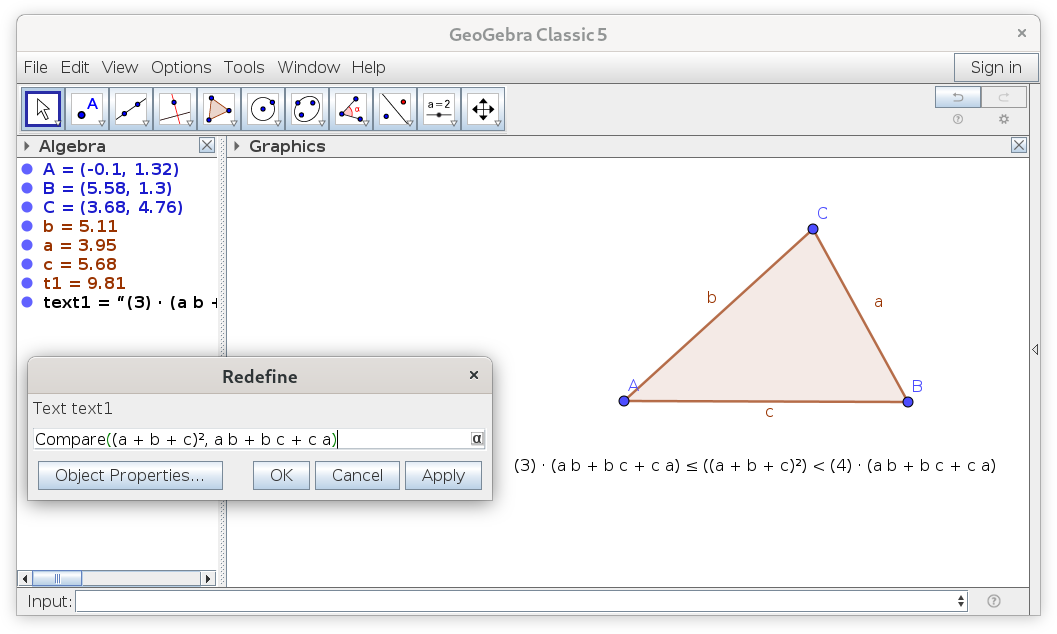
Figure 1: A mechanical solution by GeoGebra Discovery for the problem Bottema 1.1

In fact, GeoGebra Discovery is programmed to realize that the expressions $(a+b+c)^{2}$ and $ab+bc+ca$ both are homogeneous quadratic formulas.

We illustrate the same idea on an equality in a regular pentagon. In Fig. 2 a regular 5-gon $ABCDE$ is shown with the midpoint $M$ of its circumcircle. We introduce the quantities $f=AB$, $k=AC$, $l=AD$, $j=AE$, $R=AM$. After some experiments one can find that there is an interesting relationship among the product $f\cdot k\cdot l\cdot j$ and $R$. In this example, however, we use the command Relation($f\cdot k\cdot l\cdot j$,$R$) to do a numerical check first (Fig. 3(a)), and also to have a nicely looking symbolic result when clicking on the button “More$\ldots$” (Fig. 3(b)).

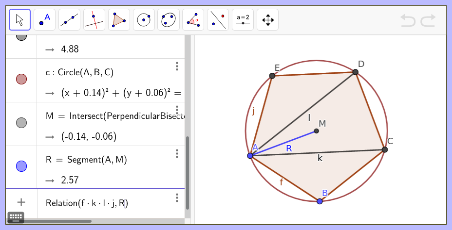
Figure 2: Using the Relation command to obtain a relationship in a regular pentagon

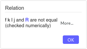
(a) Numerical check

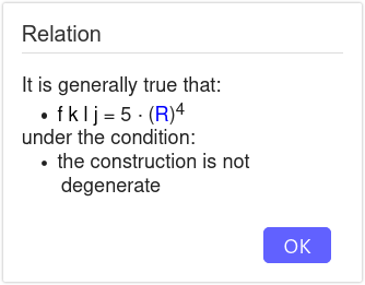
(b) Symbolic check

Figure 3: Results on comparing $f\cdot k\cdot l\cdot j$ and $R$

The Relation command in GeoGebra is a well-known way to compare two objects, from its first versions, but the comparison used to be performed only numerically. If one wants to compare just two objects (that is, not expressions, but, for example, segments), then a point-and-click comparison is also possible. This is demonstrated in Fig. 4: after selecting the Relation tool, two segments, e.g. $f$ and $k$, we learn that their ratio is $\frac{1}{2}\cdot(\sqrt{5}-1)$ or $\frac{1}{2}\cdot(\sqrt{5}+1)$ (see Fig. 5). Confusingly, it remains an unanswered question here whether the first or the second one is the correct result.

Figure 4: The Relation tool in the toolbar in GeoGebra 6

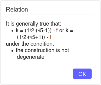
Figure 5: Symbolic relationship between the side and a diagonal of a regular pentagon

To explain this issue, we need to distinguish between two main GeoGebra versions: 5 and 6. Version 5 has support to handle inequalities, but version 6 not at the moment. In version 6 the underlying computations in the algebro-geometric setup cannot restrict the geometric figure to a single regular pentagon. Instead of a single regular polygon, all possible star-regular polygons are observed at the same time. In the case of a regular pentagon this means that the computation for a regular pentagram will also be computed—two results will be given concurrently. In general this means that the final result always includes a solution according each star-regular variant. (Fortunately, for a square or a regular hexagon there are no star-regular variants, but for a regular heptagon there are two heptagrams—so three cases are computed at the same time.)

In version 5 we are already capable of issuing a restriction that point $C$ takes place in the half-plane whose boundary line includes $B$ and is perpendicular to the segment $AB$. In this case we can exclude the pentagram variant (Fig. 6). With such considerations we can extend the equation based approach to a much broader set of applications. Among others, it is possible to attach a point on a segment or inside a triangle, or to explicitly define the center of the incircle of a triangle.

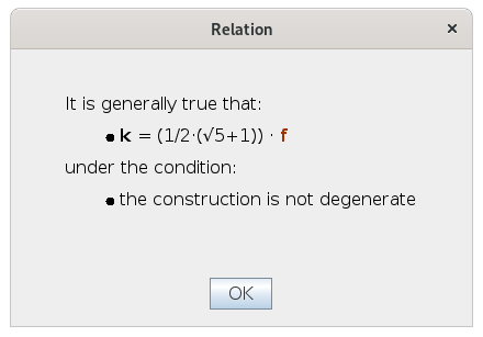
Figure 6: Unambiguous result on the ratio between the side and a diagonal of a regular pentagon (supported only in GeoGebra 5)

In the beginning of this section we mentioned the Compare command in GeoGebra Discovery, and finally we arrived to a higher level command/tool: Relation. In fact, Relation uses the internal routine of the Compare command, so, at the end of the day, the same computations are performed, independently of the launched command.

Finally we give some more description on the system layout of the above mentioned two GeoGebra versions, 5 and 6. At the moment only GeoGebra 5 (a native Java application) can give any result on inequalities, because all RQE computations are outsourced to Mathematica or Tarski. Fig. 7 gives an overview of the underlying technical hierarchy. GeoGebra internally uses the Giac computer algebra system to perform a large set of symbolic computations [GiacGG-RICAM2013].

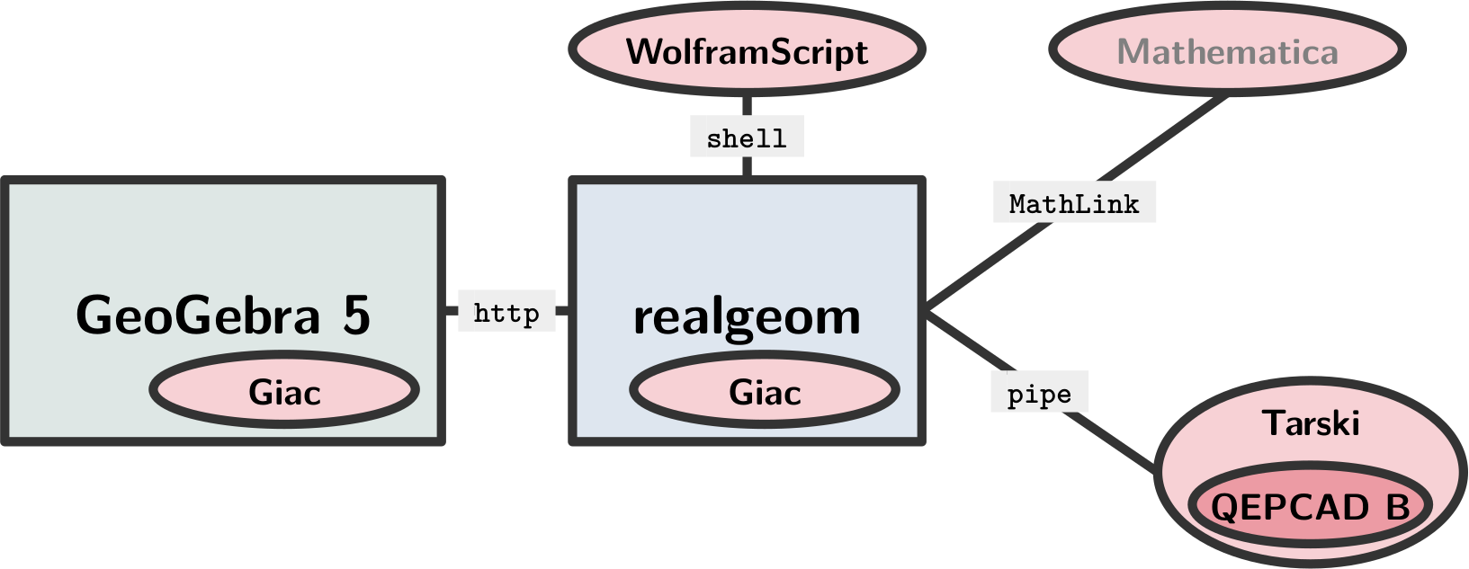
Figure 7: Computation hierarchy for GeoGebra 5

By contrast, GeoGebra 6 (a web browser based variant of GeoGebra) is capable only of obtaining equalities, because no connection has been made yet to any systems that provide RQE computations. See Fig. 8 for the simple schema being available for the moment.

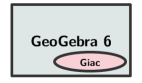
Figure 8: Computation hierarchy for GeoGebra 6

4 Mathematical background

We point the reader to the first experiments on this topic to [SturmWeispfenning96] (on proving inequalities) and [RecioVelez99] (on obtaining equalities). By using a non-trivial but still simple example we explain the main idea how our algorithms work.

The problem setting, as visible in Fig. 9, is to compare $f+g$ and $c$ in an arbitrary triangle $ABC$—here $f$ and $g$ are two medians of the triangle, and $c$ is the side of the triangle exactly as drawn in the figure. Now Fig. 10 shows how this problem is translated into an algebraic setup: each of the free points $A$, $B$ and $C$ are expressed by two coordinates ($v_{1},v_{2},v_{3},v_{4},v_{5},v_{6}$), dependent points $D$ and $E$ are given with another two times two coordinates ($v_{7},v_{8},v_{9},v_{10}$), and another three variables describe the length of $c$, $g$ and $f$ ($v_{11},v_{12},v_{13}$). All of these mappings are done automatically by GeoGebra by following a mechanical algorithm, and also some equations are set up to describe the relationships between these variables—in our case four equations will be created.

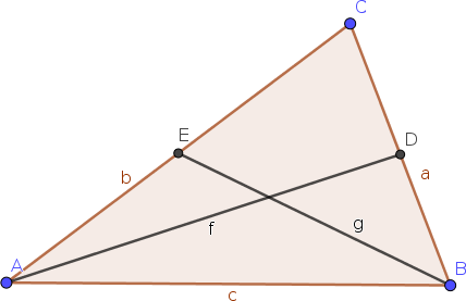
Figure 9: Problem setting

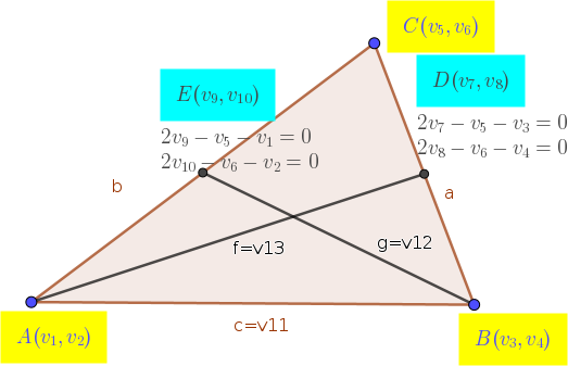
Figure 10: Algebraization of the problem setting

Four or five more technical variables are introduced:

• $v_{14}$ is used to prescribe a condition on the non-degeneracy of $ABC$, namely,

  $$v_{14}\cdot\left|\begin{matrix}v_{1}&v_{2}&1\\ v_{3}&v_{4}&1\\ v_{5}&v_{6}&1\end{matrix}\right|-1=0,$$

  by using the Rabinowitsch trick [Rabinowitsch1929]. Here the geometrical meaning is an inequation, even if we use an equation for its algebraic translation. This ensures that only algebraic equations are set up in the first round and no algebraic inequality will be present. To use effective elimination via Gröbner bases this step cannot be avoided.

• $w_{1}$ and eventually $w_{2}$ are used to describe the two expressions with a single variable, respectively.

• $m$ plays the role of $m$, $M$ and $\mu$ as explained above.

• $n$ is used to express that one of the two expressions differs from $0$. Here, again, the Rabinowitsch trick is used.

After these settings GeoGebra uses elimination first if a suitable $\mu$ exists. To achieve this, the following Giac code is executed:

⬇

[assume(m>0),solve(eliminate(subst([2*v7-v5-v3,2*v8-v6-v4,2*v9-v5-v1,2*v10-v6-v2,-v12^2+v10^2+v9^2-2*v10*v4+v4^2-2*v9*v3+v3^2,-v11^2+v4^2+v3^2-2*v4*v2+v2^2-2*v3*v1+v1^2,-v13^2+v8^2+v7^2-2*v8*v2+v2^2-2*v7*v1+v1^2,-1-v14*v5*v4+v14*v6*v3+v14*v5*v2-v14*v3*v2-v14*v6*v1+v14*v4*v1,-w1+(v13+v12)^1,v11*m-(w1),(v11)*n-1],[v1=0,v2=0,v3=1,v4=0]),[v1,v2,v3,v4,v5,v6,v7,v8,v9,v10,v11,v12,v13,v14,w1,n])[0],m)][1]

We note that the first free two points are positioned to $(0,0)$ and $(1,0)$, respectively. This is allowed without loss of generality—with the assumption that the algorithm always verifies if the expressions are homogeneous and of the same degree. (See also [Davenport2017].)

If Giac gave a non-erroneous output here, then we managed to find the sought $\mu$ (or, eventually a set of possible values for $\mu$). Otherwise there is a second round needed—like in our case in this example. GeoGebra now outsources the problem to a realgeom server, by composing an http request, something like http://192.168.10.20:8765/euclideansolver?lhs=w1&rhs=v11&polys=2*v7-v5-v3,2*v8-v6-v4,2*v9-v5-v1,2*v10-v6-v2,-v12This triggers realgeom's internal computations that finally launch a request towards Mathematica (or Tarski) like this: