Turbulence via intermolecular potential:
Viscosity and transition range of the Reynolds number

Abstract.

Turbulence in fluids is an ubiquitous phenomenon, characterized by spontaneous transition of a smooth, laminar flow to rapidly changing, chaotic dynamics. In 1883, Reynolds experimentally demonstrated that, in an initially laminar flow of water, turbulent motions emerge without any measurable external disturbance. To this day, turbulence remains a major unresolved phenomenon in fluid mechanics; in particular, there is a lack of a mathematical model where turbulent dynamics emerge naturally from a laminar flow. Recently, we proposed a new theory of turbulence in gases, according to which turbulent motions are created in an inertial gas flow by the mean field effect of the intermolecular potential. In the current work, we investigate the effect of viscosity in our turbulence model, by numerically simulating the air flow at normal conditions in a straight pipe for different values of the Reynolds number. We find that the transition between the laminar and turbulent flows in our model occurs without any deliberate perturbations as the Reynolds number increases from 2000 to 4000. As the simulated flow becomes turbulent, the decay rate of the time averaged Fourier spectrum of the kinetic energy in our model approaches Kolmogorov’s inverse five-thirds law. Both results are consistent with experiments and observations.

1. Introduction

Historically, the phenomenon of turbulence in fluids has been noted by Leonardo da Vinci. However, its first scientifically documented account appears to be due to Boussinesq [1], while the word “turbulence” itself has been suggested by Thomson [2]. In his famous experiment, Reynolds [3] demonstrated that a laminar flow of water spontaneously developed turbulent motions without any measurable external disturbances, and that the onset of turbulence was reliably associated with a sufficiently high value of the Reynolds number. Later, Kolmogorov [4, 5, 6] found that the time-averaged Fourier spectrum of the kinetic energy of turbulent air flow decayed as the inverse five-thirds power of its wavenumber.

Despite overwhelming research efforts spanning multiple decades [7, 8, 9, 10, 11, 12, 13, 14, 15, 16, 17, 18, 19, 20, 21, 22, 23], the phenomenon of turbulence in gases and liquids remains unexplained; namely, there does not exist an adequate fluid-mechanical model, for either a liquid or a gas, where, at appropriate values of the Reynolds number, turbulent flow naturally emerges from laminar initial and boundary conditions in the absence of artificial external disturbances. As examples, one can refer to recent works by Avila et al. [24], Barkley et al. [25] and Khan et al. [26], where turbulent-like motions in a numerically simulated flow had to be created artificially by deliberate perturbations. In reality, turbulence emerges spontaneously by itself, even if all reasonable measures were taken to preserve the laminarity of the flow (e.g. the experiment of Reynolds [3]) – moreover, it was precisely the spontaneity of the onset of turbulence which attracted the world-wide scientific interest to this intriguing phenomenon. Also, numerical simulations of artificially disturbed flows using conventional equations of fluid mechanics fail to capture Kolmogorov’s power scaling of the kinetic energy spectra [26].

In our recent works [27, 28, 29] we proposed a theory of turbulence in a gas, where turbulent motions in an initially laminar, inertial (that is, constant pressure) flow were created via the average effect of gas molecules interacting by means of their intermolecular potential $\phi(r)$. In our theory, this average effect is expressed via the mean field potential $\bar{\phi}$ (which, of course, depends on $\phi(r)$), whose gradient enters the equation for the transport of momentum. According to our theory, in the absence of the pressure gradient, the effect of $\bar{\phi}$ becomes the key driving force of turbulent dynamics. This novel effect is absent from the conventional Euler and Navier–Stokes equations of fluid mechanics because, in the Boltzmann–Grad limit [30], it is tacitly assumed that the effect of $\bar{\phi}$ is negligible. However, we found that, in our model of inertial gas flow, $\bar{\phi}$ produces turbulent flow with Kolmogorov decay of the Fourier spectra of the kinetic energy. Evidently, its effect is non-negligible and quantifiable.

Remarkably, Tsugé [31] attempted to explain the creation of turbulence via long-range correlations between molecules, but Tsugé’s result was restricted to an incompressible flow. On the other hand, from what we discovered thus far, it appears that density fluctuations are instrumental in the creation of turbulent dynamics. In our past work [32], we also considered long-range interactions as a possible reason for the manifestation of turbulence. However, we later found that even the hard sphere potential creates turbulence in our model, which means that a typical intermolecular potential is also capable of the same effect.

Thus far, our model of turbulent gas flow did not include viscous effects. In the current work, we equip the momentum transport equation of our model with the standard viscous term, which counteracts the effect of the mean field potential (i.e. $\bar{\phi}$ creates turbulent motions, while the viscosity dissipates them). We numerically simulate the air flow at normal conditions within a straight pipe at different values of the Reynolds number, and find that the transition between the laminar and turbulent flow in our model occurs within the same range of values of the Reynolds number as observed in practice [33, 34]. Additionally, we find that, for turbulent values of the Reynolds number, the rate of decay of the time-averaged Fourier spectrum of the kinetic energy of the flow approaches the famous Kolmogorov decay rate of the inverse five-thirds power of the wavenumber.

The work is organized as follows. In Section 2, we present the inviscid model of inertial flow with the mean field potential, and demonstrate that, at a low Mach number, the effect of the mean field potential in nondimensional variables is of the same order as the rest of the terms. In Section 3, we add viscosity into the momentum equation in a standard fashion. In Section 4, we present the results of a numerical simulation of the air flow at normal conditions in a straight pipe, and show that the laminar-to-turbulent transition occurs as the Reynolds number increases from 2000 to 4000. Section 5 summarizes the results of this work.

2. Our model of inertial turbulent gas flow

In the context of our theory [27, 28, 29], the turbulent flow of a gas with density $\rho$ and velocity $\boldsymbol{u}$, at a constant pressure $p_{0}$ (inertial flow) and in the absence of viscous effects, is described by the following mass and momentum transport equations

(1) $$\frac{\partial\rho}{\partial t}+\nabla\cdot(\rho\boldsymbol{u})=0,$$

(2) $$\frac{\partial(\rho\boldsymbol{u})}{\partial t}+\nabla\cdot(\rho\boldsymbol{u}^{2})+\nabla\bar{\phi}=\boldsymbol{0}.$$

Above, observe that the momentum transport equation (2) possesses a novel term $\nabla\bar{\phi}$, which replaces the pressure gradient in the conventional Euler or Navier–Stokes equations. This term quantifies the average (or mean field) effect of the motion of molecules of mass $m$, interacting via a potential $\phi(r)$. Therefore, in our preceding works we referred to $\bar{\phi}$ as the mean field potential.

Assuming that the intermolecular potential $\phi(r)$ has the effective range $\sigma$, we estimated the mean field potential $\bar{\phi}$ via

(3) $$\bar{\phi}=4p_{0}\rho/\rho_{H\!\!\;S},$$

where $\rho_{H\!\!\;S}=6m/\pi\sigma^{3}$ is the density of the equivalent hard sphere of mass $m$ and diameter $\sigma$. Substituting $\bar{\phi}$ from (3) into (2) yields

(4) $$\frac{\partial(\rho\boldsymbol{u})}{\partial t}+\nabla\cdot(\rho\boldsymbol{u}^{2})+\frac{4p_{0}}{\rho_{H\!\!\;S}}\nabla\rho=\boldsymbol{0}.$$

This novel effect is absent from the conventional Euler and Navier–Stokes equations of fluid mechanics because, in the Boltzmann–Grad hydrodynamic limit (see Grad [30], pp. 352–353), it is assumed that $\sigma^{2}/m\sim$ constant as $m$ and $\sigma$ are taken to zero, and therefore, $\rho_{H\!\!\;S}\to\infty$. However, it can be shown that, in the nondimensional variables, the effect of the mean field potential in the inertial flow is comparable to the rest of the terms at sufficiently low Mach numbers. In order to see this, we rescale the variables in (1) and (4) in a standard fashion, by introducing the reference values of spatial scale $L$, flow speed $U$, and density $\rho_{0}$:

(5) $$\tilde{t}=Ut/L,\qquad\tilde{\boldsymbol{x}}=\boldsymbol{x}/L,\qquad\tilde{\rho}=\rho/\rho_{0},\qquad\tilde{\boldsymbol{u}}=\boldsymbol{u}/U.$$

In addition, we denote the packing fraction $\eta$ and the Mach number $\mathit{Ma}$ via

(6) $$\eta=\rho_{0}/\rho_{H\!\!\;S},\qquad\mathit{Ma}=U\sqrt{\rho_{0}/\gamma p_{0}},$$

where $\gamma$ is the adiabatic exponent of the gas. In the nondimensional variables, the density equation (1) remains the same, while the momentum equation (4) becomes

(7) $$\frac{\partial(\tilde{\rho}\tilde{\boldsymbol{u}})}{\partial\tilde{t}}+\tilde{\nabla}\cdot(\tilde{\rho}\tilde{\boldsymbol{u}}^{2})+\alpha\tilde{\nabla}\tilde{\rho}=\boldsymbol{0},\qquad\alpha=\frac{4\eta}{\gamma\mathit{Ma}^{2}}.$$

For air, $\gamma=1.4$, and $\rho_{H\!\!\;S}=1850$ kg/m³ (see Eq. (64) in our work [28] for details). At normal conditions (sea level, 20^∘C), we have $\rho_{0}=1.204$ kg/m³, and $p_{0}=101.3$ kPa. As a result, the packing fraction $\eta\approx 6.5\cdot 10^{-4}$. Also, taking $U=30$ m/s, as in the numerical simulations below, we obtain $\mathit{Ma}\approx 8.74\cdot 10^{-2}$. Combining the estimates, we arrive at $\alpha\approx 0.24$, for the settings of our numerical simulations below. Moreover, reducing the speed of the flow to 15 m/s leads to $\alpha\approx 1$. This confirms that the mean field effect of the intermolecular potential at normal conditions and relatively low Mach numbers is not negligible, and certainly does not vanish as presumed in the Boltzmann–Grad limit.

3. A model of inertial turbulent gas flow with viscosity

Due to the absence of viscosity, numerical solutions of equations (1) and (4) always develop turbulent dynamics from an initially laminar flow [27, 28, 29]. In the current work, we add the standard viscous term with the dynamic viscosity $\mu$ into the momentum equation (4):

(8) $$\frac{\partial(\rho\boldsymbol{u})}{\partial t}+\nabla\cdot(\rho\boldsymbol{u}^{2})+\frac{4p_{0}}{\rho_{H\!\!\;S}}\nabla\rho=\nabla\cdot(\mu\nabla\boldsymbol{u}).$$

According to the kinetic theory of gases [35], $\mu$ is proportional to the square root of the temperature. In a gas, the product of temperature and density is proportional to the pressure, which, in turn, is constant in an inertial gas flow. Therefore, in our setting,

(9) $$\mu=\mu_{0}\sqrt{\rho_{0}/\rho},$$

where $\mu_{0}$ is the reference value of viscosity. In the nondimensional variables, (8) becomes

(10) $$\frac{\partial(\tilde{\rho}\tilde{\boldsymbol{u}})}{\partial\tilde{t}}+\tilde{\nabla}\cdot(\tilde{\rho}\tilde{\boldsymbol{u}}^{2})+\alpha\tilde{\nabla}\tilde{\rho}=\frac{1}{\mathit{Re}}\tilde{\nabla}\cdot\big{(}\tilde{\rho}^{-1/2}\tilde{\nabla}\tilde{\boldsymbol{u}}\big{)},$$

where the Reynolds number $\mathit{Re}$ is given via

(11) $$\mathit{Re}=\rho_{0}UL/\mu_{0}.$$

It is clear that, in this model, turbulent flow cannot emerge if the coefficients of the forcing and dissipative terms are balanced, that is, $\mathit{Re}=\alpha^{-1}\approx 4.1$ in our setting. However, for $\mathit{Re}\gg\alpha^{-1}$, the manifestation of turbulent flow depends on the geometry of the domain. In particular, it is known from observations and practical engineering knowledge [33], that the transition between laminar and turbulent gas flow in straight pipes occurs within the range of values of the Reynolds number between 2000 and 4000, with the parameters $L$ and $U$ in (11) being the width of the pipe, and the maximum speed of the flow, respectively.

We have to note that, in general, the presence of viscosity in a flow induces pressure variations due to viscous friction; yet, above we introduced viscosity into the momentum transport equation (8) rather formally, without accounting for such an effect. Thus, the system of transport equations for the density (1) and momentum (8) should not be viewed as a practical method for accurate prediction of a real-world gas flow. Instead, it should be treated as a “proof-of-concept” model, whose purpose is to investigate how the relation between the mean field potential forcing and viscous dissipation alone results in the manifestation of turbulence in a gas flow, and at which values of the Reynolds number such a transition occurs.

To confirm that our model is suitable for the above stated purpose, first observe that, in an established laminar solution of the conventional Navier–Stokes system, expressed in the nondimensional variables, the term with the pressure gradient, induced by the viscous friction, must be comparable to the viscous term itself (that is, $\sim\mathit{Re}^{-1}$). In the numerical simulations below, we find that a laminar flow still develops for $\mathit{Re}=1000$, which is also the smallest value of the Reynolds number used. This, in turn, means that, for $\alpha\approx 0.24$ in (10), the effect of the induced pressure gradient would be $\sim$ 240 times smaller than that of the mean field potential term, and could, therefore, be disregarded.

4. Numerical simulations

To investigate whether or not our model predicts the transition to a turbulent flow within a realistic range of values of the Reynolds number, here we present numerical simulations of an inertial air flow at normal conditions in a straight pipe. As in our recent works, we use the appropriately modified rhoCentralFoam solver [36], which uses the central discretization scheme of Kurganov and Tadmor [37], with the flux limiter due to van Leer [38]. The rhoCentralFoam solver is a standard component of the OpenFOAM suite [39].

Here, we simulate the inertial air flow in a straight pipe of a square cross-section, using equations (1) and (8), with $p_{0}=101.3$ kPa, and $\rho_{H\!\!\;S}=1850$ kg/m³. The size of the pipe is $36\times 5.2\times 5.2$ cm³. The domain is uniformly discretized in all directions with the step of $0.8$ mm, which comprises $450\times 65\times 65=1,901,250$ finite volume cells in total. The pipe is open-ended at the outlet side, and has a wall at the inlet side, with the circular inlet of 1 cm in diameter located in the middle of this wall. The longitudinal section of the domain is shown in Figure 1.

The boundary conditions are the following. The density is set to $\rho=1.204$ kg/m³ at the outlet, and has zero normal derivative at the inlet and the walls. The velocity has zero normal derivative at the outlet, no-slip condition at the walls, and a radially symmetric parabolic profile at the inlet, with the maximum of 30 m/s in the middle of the inlet, directed along the axis of the pipe. The diameter of the inlet, and the speed of the entering flow correspond to the experiment by Buchhave and Velte [40]. Initially, the gas inside the pipe is at rest, with zero velocity and uniform density set to 1.204 kg/m³.

We conducted numerical simulations of (1) and (8) for the values of the Reynolds number $\mathit{Re}=1000$, $2000$, $3000$ and $4000$, by setting the reference viscosity $\mu_{0}$ to $1.872\cdot 10^{-3}$, $9.36\cdot 10^{-4}$, $6.24\cdot 10^{-4}$ and $4.68\cdot 10^{-4}$ kg/m s, respectively. We integrated equations (1) and (8) forward in time using the explicit (forward Euler) scheme for the advection and mean field potential forcing terms, and implicit (backward Euler) scheme for the viscous term. The forward time stepping of the scheme was adaptive, with the time step set to 20% of the maximal allowed by the Courant number.

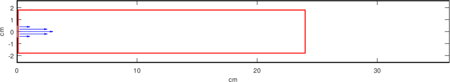
Figure 1. Longitudinal section of the computational domain. The domain dimensions are $36\times 5.2\times 5.2$ cm³. The inlet is on the left, and the outlet is on the right. The pipe walls are shown via thick black lines, so that both the inlet and outlet are visible. The boundary of the Fourier spectrum measurement region is shown in red. This region is a box of 24 cm in length, and $3.6\times 3.6$ cm² in cross-section.

Here, observe that the goal of the simulation is not the local accuracy of the solution, but rather the accurate capture of the statistical regime of the dynamics (and, in particular, the transition to nonlinear chaos). This means that the numerical integration scheme should be chosen so as to avoid the introduction of artificial damping into the advection part of the system. Due to this reason, the simple forward Euler method appears to be better for such a specific purpose than more advanced numerical integration schemes, such as the 4th order Runge–Kutta method, since the latter tend to introduce artificial damping into numerical solutions as a result of their superior stability properties [41].

4.1. Results

We found that the flow fully developed by the elapsed time $t=0.07$ seconds in all simulations. In Figure 2, we show four snapshots of the speed of the flow, taken in the longitudinal symmetry plane of the pipe at $t=0.15$ s, which illustrate the transition between the laminar and turbulent flow. For $\mathit{Re}=1000$, the flow is laminar, as evidenced by smoothness of the level curves, and symmetric relative to the axis of the pipe. For $\mathit{Re}=2000$, the symmetry of the flow is broken, and small intermittent fluctuations appear in the otherwise laminar flow. These fluctuations become larger and more numerous for $\mathit{Re}=3000$; for $\mathit{Re}=4000$, the flow is fully turbulent. Clearly, the range of values of the Reynolds number, at which the turbulent transition occurs in our model, agrees with observations [33]. The breaking of the flow symmetry during the transition to turbulence is likely associated with the onset of chaos in the dynamics, and, in numerical simulations, happens due to exponentially growing machine round-off errors. The hypothesis that turbulence is a manifestation of nonlinear chaos has also been discussed in the literature (see Letellier [34] and references therein).

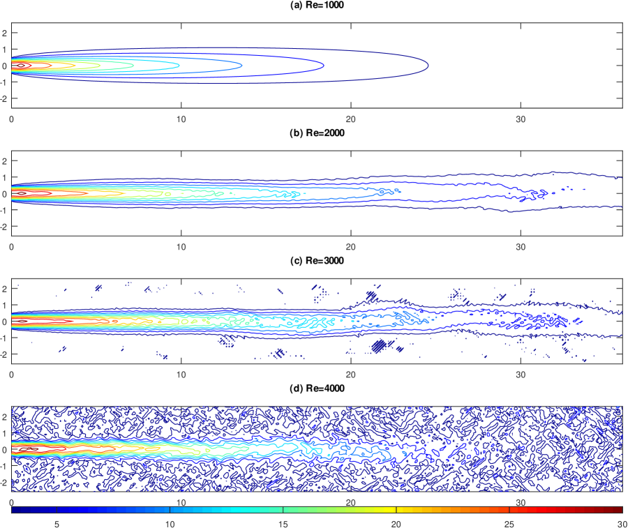
Figure 2. Speed of the flow (m/s), expressed in the form of level curves, and captured in the longitudinal symmetry plane of the pipe at the elapsed time $t=0.15$ s for (a) $\mathit{Re}=1000$, (b) $\mathit{Re}=2000$, (c) $\mathit{Re}=3000$ and (d) $\mathit{Re}=4000$.

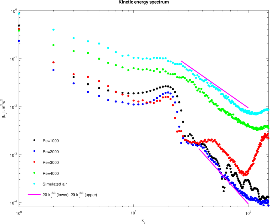
Figure 3. The Fourier spectra of the kinetic energy, averaged between $0.1$ and $0.2$ s of the elapsed time, for $\mathit{Re}=1000$, $2000$, $3000$ and $4000$, as well as air ($\mu_{0}=1.825\cdot 10^{-5}$ kg/m s). The power decay slopes $E_{0}k_{x}^{-5/3}$ and $E_{0}k_{x}^{-8/3}$, with $E_{0}=20$ m²/s², are added for reference.

In addition to the snapshots of the speed of the flow, we computed the time averages of its kinetic energy spectrum. The computation was done within the central core of the pipe of $3.6\times 3.6$ cm² in cross-section, extending between 0 and 24 cm of the length of the pipe (shown in red in Figure 1), and thus largely containing the jet stream. The time averaging was carried out in the interval between $0.1$ and $0.2$ seconds of the elapsed time. For the detailed description of the energy spectrum computation, see our recent works [27, 28, 29].

In Figure 3, we show time averages of the computed Fourier spectra of the streamwise component of the kinetic energy for the same simulated flows, which are displayed as functions of their Fourier wavenumber $k_{x}$ in the longitudinal direction of the pipe on a logarithmic scale. In addition, we show the kinetic energy spectrum for the simulation with $\mu_{0}=1.825\cdot 10^{-5}$ kg/m s ($\mathit{Re}\sim 10^{5}$), which corresponds to the viscosity of air at normal conditions. For the reference, we show two power slope lines, given via $E_{0}k_{x}^{-8/3}$ and $E_{0}k_{x}^{-5/3}$, which share the same empirically chosen scaling constant $E_{0}=20$ m²/s².

At the large scale Fourier wavenumbers, the structures of the kinetic energy spectra of all computed flows are similar, while the major differences are observed at moderate and small scales. For $\mathit{Re}=1000$, $2000$ and $3000$, the kinetic energy spectrum at small scales generally appears to match the $k^{-8/3}$-decay slope, with the following variations. In the $\mathit{Re}=2000$ regime, the spectrum decays along the $k^{-8/3}$-slope rather monotonously, whereas in the $\mathit{Re}=1000$ regime (which is fully laminar) the spectrum also exhibits oscillations around this slope. As we hypothesized in [29], the latter could be a manifestation of the quasi-periodic dynamics at the unstable Fourier wavenumbers, with the periodicity of orbits destroyed by chaos as $\mathit{Re}$ increases to 2000. In the regime with $\mathit{Re}=3000$, an unusual growth of the energy spectrum is observed at small scales. Remarkably, the rate of decay of the kinetic energy spectrum for the turbulent regime $\mathit{Re}=4000$, as well as that of the air, approach Kolmogorov’s $k^{-5/3}$-slope.

5. Summary

In the current work, we formally introduce viscosity into our model of turbulence via an intermolecular potential [27, 28, 29], to investigate the transition between laminar and turbulent air flows with varying Reynolds number. We numerically simulate the air flow at normal conditions in a straight pipe at different values of the Reynolds number, and find that the transition into turbulent flow occurs when the Reynolds number increases from 2000 to 4000. This appears to be consistent with observations, experiments and practical knowledge. Additionally, we find that, in our model, the corresponding rate of decay of the time-averaged Fourier transform of the streamwise kinetic energy at small scales changes from $k^{-8/3}$-slope towards $k^{-5/3}$-slope (Kolmogorov’s law), as the flow transitions from laminar to turbulent.

The results of our work seem to be encouraging. For the first time in history, we created a model of compressible gas flow in the form of fluid mechanics equations, where, first, turbulent dynamics emerge from an initially laminar flow at appropriate values of the Reynolds number naturally and without the help of artificial disturbances, and, second, the rate of decay of the Fourier spectrum of the kinetic energy of turbulent flow in our model matches that observed in nature.

At the same time, our model has its limitations, as it describes the inertial gas flow; in a realistic flow, the pressure generally fluctuates, even if slightly. However, other models of fluid mechanics have their own limitations – for example, both the incompressible and compressible Euler equations are incompatible with the process of convection (the density is constant in the former, and increases when the air warms up in the latter). Yet, such models are widely used, because they describe specific features of the flow which are needed for relevant practical applications. Similarly, our model may find its own use – perhaps, as a “stepping stone”, improving our general understanding of the fluid mechanics of turbulence.

Acknowledgment

This work was supported by the Simons Foundation grant #636144.

References

- Boussinesq [1877] J. Boussinesq. Essai sur la théorie des eaux courantes. Mémoires présentés par divers savants à l’Académie des Sciences, XXIII(1):1–680, 1877.
- Thomson [1887] W. Thomson. XLV. On the propagation of laminar motion through a turbulently moving inviscid liquid. Philos. Mag. Series 5, 24(149):342–353, 1887.
- Reynolds [1883] O. Reynolds. An experimental investigation of the circumstances which determine whether the motion of water shall be direct or sinuous, and of the law of resistance in parallel channels. Proc. R. Soc. Lond., 35(224–226):84–99, 1883.
- Kolmogorov [1941a] A.N. Kolmogorov. Decay of isotropic turbulence in an incompressible viscous fluid. Dokl. Akad. Nauk SSSR, 31:538–541, 1941a.
- Kolmogorov [1941b] A.N. Kolmogorov. Energy dissipation in locally isotropic turbulence. Dokl. Akad. Nauk SSSR, 32:19–21, 1941b.
- Kolmogorov [1941c] A.N. Kolmogorov. Local structure of turbulence in an incompressible fluid at very high Reynolds numbers. Dokl. Akad. Nauk SSSR, 30:299–303, 1941c.
- Reynolds [1895] O. Reynolds. On the dynamical theory of incompressible viscous fluids and the determination of the criterion. Phil. Trans. Roy. Soc. A, 186:123–164, 1895.
- Richardson [1926] L.F. Richardson. Atmospheric diffusion shown on a distance-neighbour graph. Proc. Roy. Soc. London A, 110:709–737, 1926.
- Taylor [1935] G.I. Taylor. Statistical theory of turbulence. Proc. Roy. Soc. London A, 151(873):421–444, 1935.
- Taylor [1938] G.I. Taylor. The spectrum of turbulence. Proc. Roy. Soc. London A, 164:476–490, 1938.
- von Kármán and Howarth [1938] T. von Kármán and L. Howarth. On the statistical theory of isotropic turbulence. Proc. Roy. Soc. London A, 164:192–215, 1938.
- Prandtl [1938] L. Prandtl. Beitrag zum Turbulenzsymposium. In J.P. Den Hartog and H. Peters, editors, Proceedings of the Fifth International Congress on Applied Mechanics, pages 340–346, Cambridge MA, 1938. John Wiley, New York.
- Obukhov [1941] A.M. Obukhov. On the distribution of energy in the spectrum of a turbulent flow. Izv. Akad. Nauk SSSR Ser. Geogr. Geofiz., 5:453–466, 1941.
- Obukhov [1949] A.M. Obukhov. Structure of the temperature field in turbulent flow. Izv. Akad. Nauk SSSR Ser. Geogr. Geofiz., 13:58–69, 1949.
- Chandrasekhar [1949] S. Chandrasekhar. On Heisenberg’s elementary theory of turbulence. Proc. Roy. Soc., 200:20–33, 1949.
- Corrsin [1951] S. Corrsin. On the spectrum of isotropic temperature fluctuations in an isotropic turbulence. J. Appl. Phys., 22(4):469–473, 1951.
- Kolmogorov [1962] A.N. Kolmogorov. A refinement of previous hypotheses concerning the local structure of turbulence in a viscous incompressible fluid at high Reynolds number. J. Fluid Mech., 13(1):82–85, 1962.
- Obukhov [1962] A.M. Obukhov. Some specific features of atmospheric turbulence. J. Geophys. Res., 67(8):3011–3014, 1962.
- Kraichnan [1966a] R.H. Kraichnan. Dispersion of particle pairs in homogeneous turbulence. Phys. Fluids, 9:1937–1943, 1966a.
- Kraichnan [1966b] R.H. Kraichnan. Isotropic turbulence and inertial range structure. Phys. Fluids, 9:1728–1752, 1966b.
- Saffman [1967] P.G. Saffman. The large-scale structure of homogeneous turbulence. J. Fluid Mech., 27(3):581–593, 1967.
- Saffman [1970] P.G. Saffman. A model for inhomogeneous turbulent flow. Proc. Roy. Soc. London A, 317:417–433, 1970.
- Mandelbrot [1974] B.B. Mandelbrot. Intermittent turbulence in self-similar cascades; divergence of high moments and dimension of the carrier. J. Fluid Mech., 62(2):331–358, 1974.
- Avila et al. [2011] K. Avila, D. Moxey, A. de Lozar, M. Avila, D. Barkley, and B. Hof. The onset of turbulence in pipe flow. Science, 333:192–196, 2011.
- Barkley et al. [2015] D. Barkley, B. Song, V. Mukund, G. Lemoult, M. Avila, and B. Hof. The rise of fully turbulent flow. Nature, 526:550–553, 2015.
- Khan et al. [2021] H.H. Khan, S.F. Anwer, N. Hasan, and S. Sanghi. Laminar to turbulent transition in a finite length square duct subjected to inlet disturbance. Phys. Fluids, 33:065128, 2021.
- Abramov [2021a] R.V. Abramov. Macroscopic turbulent flow via hard sphere potential. AIP Adv., 11(8):085210, 2021a.
- Abramov [2021b] R.V. Abramov. Turbulence in large-scale two-dimensional balanced hard sphere gas flow. Atmosphere, 12(11):1520, 2021b.
- Abramov [2022] R.V. Abramov. Creation of turbulence in polyatomic gas flow via an intermolecular potential. Preprint: https://arxiv.org/abs/2201.07175, 2022.
- Grad [1949] H. Grad. On the kinetic theory of rarefied gases. Comm. Pure Appl. Math., 2(4):331–407, 1949.
- Tsugé [1974] S. Tsugé. Approach to the origin of turbulence on the basis of two-point kinetic theory. Phys. Fluids, 17(1):22–33, 1974.
- Abramov [2020] R.V. Abramov. Turbulent energy spectrum via an interaction potential. J. Nonlinear Sci., 30:3057–3087, 2020.
- Menon [2005] E.S. Menon. Gas Pipeline Hydraulics. Taylor & Francis, Boca Raton, FL, 2005.
- Letellier [2017] C. Letellier. Intermittency as a transition to turbulence in pipes: A long tradition from Reynolds to the 21st century. C.R. Mecanique, 345:642–659, 2017.
- Hirschfelder et al. [1964] J.O. Hirschfelder, C.F. Curtiss, and R.B. Bird. The Molecular Theory of Gases and Liquids. Wiley, 1964.
- Greenshields et al. [2010] C.J. Greenshields, H.G. Weller, L. Gasparini, and J.M. Reese. Implementation of semi-discrete, non-staggered central schemes in a colocated, polyhedral, finite volume framework, for high-speed viscous flows. Int. J. Numer. Methods Fluids, 63(1):1–21, 2010.
- Kurganov and Tadmor [2001] A. Kurganov and E. Tadmor. New high-resolution central schemes for nonlinear conservation laws and convection–diffusion equations. J. Comput. Phys., 160:241–282, 2001.
- van Leer [1974] B. van Leer. Towards the ultimate conservative difference scheme, II: Monotonicity and conservation combined in a second order scheme. J. Comput. Phys., 17:361–370, 1974.
- Weller et al. [1998] H.G. Weller, G. Tabor, H. Jasak, and C. Fureby. A tensorial approach to computational continuum mechanics using object-oriented techniques. Computers in Physics, 12(6):620–631, 1998.
- Buchhave and Velte [2017] P. Buchhave and C.M. Velte. Measurement of turbulent spatial structure and kinetic energy spectrum by exact temporal-to-spatial mapping. Phys. Fluids, 29(8):085109, 2017.
- Yu et al. [1992] S.-T. Yu, Y.-L.P. Tsai, and K.C. Hsieh. Runge–Kutta methods combined with compact difference schemes for the unsteady Euler equations. In 28th Joint Propulsion Conference and Exhibit, pages 1–28. AIAA, SAE, ASME, and ASEE, 1992.