Coasian Dynamics under Informational Robustness

Abstract

This paper studies durable goods monopoly without commitment under an informationally robust objective. A seller cannot commit to future prices and does not know the information arrival process according to which a representative buyer learns about her valuation. To avoid known conceptual difficulties associated with formulating a dynamically-consistent maxmin objective, we posit the seller’s uncertainty is resolved by an explicit player (nature) who chooses the information arrival process adversarially and sequentially. Under a simple transformation of the buyer’s value distribution, the solution (in the gap case) is payoff-equivalent to a classic environment where the buyer knows her valuation at the beginning. This result immediately delivers a sharp characterization of the equilibrium price path. Furthermore, we provide a (simple to check and frequently satisfied) sufficient condition which guarantees that no arbitrary (even dynamically-inconsistent) information arrival process can lower the seller’s profit against this equilibrium price path. We call a price path with this property a reinforcing solution, and suggest this concept may be of independent interest as a way of tractably analyzing limited commitment robust objectives. We consider alternative ways of specifying the robust objective, and also show that the analogy to known-values in the no-gap case need not hold in general.

ntroduction

Consider an interaction between a single seller and a single buyer of a durable good, where the uninformed seller makes offers to the buyer over time and only has the ability to commit to the price in the current period. The large literature on the Coase conjecture gives sharp predictions about what the equilibrium looks like when the buyer is perfectly informed regarding his willingness-to-pay (or value), at least in the “gap case”: the seller should be expected to implement a declining price path, with the market clearing in finite time. Intuitively, the seller’s lack of commitment implies that he is unable to keep the price constant over time and not cannibalize residual demand when the opportunity arises. But as the buyer anticipates future price drops, she has an additional incentive to delay purchase, which induces the seller to also lower the price in the initial period. Provided that the players are sufficiently patient, the above mechanism unravels to the point where the seller charges an initial price close to the lowest possible buyer value and obtains arbitrarily low (expected discounted) profit in equilibrium, as Coase conjectured.

The starting point for our paper is the observation that when the buyer learns about her value over time, then the classic predictions regarding equilibrium price paths can lose all sharpness. As an example, suppose that the seller is introducing a new TV, and that the buyer is completely uninformed regarding its novelty or relative value over her current TV. Suppose further that this buyer expects the seller to charge constant prices, but she reacts to a surprise deviation from the seller by learning more about what makes this TV different. We show in Proposition 2 below that there exist equilibria of this form that completely undo the Coasian predictions. Even in the gap case, we find a multiplicity of equilibria in which the seller uses a constant price path and the market fails to clear in finite time with probability one. These equilibria also support a broad range of seller payoffs. Intuitively, these equilibria leverage buyer information as an additional “punishment” that deters the seller from deviating. Of course, the complete reversal of Coasian forces as described above may not emerge in every particular informational environment. But as we discuss below in the literature review, past work on Coasian dynamics has pointed to similar failures of the Coase conjecture in the presence of buyer learning.

In this paper, we do not specify an informational environment but instead study what happens if the seller is completely ignorant about how the buyer learns her value. For instance, the buyer may be perfectly informed initially, may only learn at some later date, may learn according to the information arrival process in the previous paragraph, or each of these (or any arbitrary information arrival process) with some probability. A standard way of modeling “complete ignornace” is to assume that the seller seeks to maximize the worst-case profit guarantee across all informational environments, as in the literature on robust mechanism design. We want to understand how a seller with such a worst-case objective in mind would set prices – do non-Coasian dynamics also arise when the seller is uncertain about the buyer’s learning process, similar to the previously studied case where buyer learning is known?

To answer this question, we first introduce a novel framework for modeling a seller who does not have commitment, but still wants to set prices with worst-case scenarios in mind. In the prior literature, there does not appear to be any consensus way of doing robust mechanism design under limited commitment. As Carroll (2019) notes, “trying to write dynamic models with non-Bayesian decision makers leads to well-known problems of dynamic inconsistency, except in special cases (e.g., Epstein and Schneider (2007)). This may be one reason why there has been relatively little work to date on robust mechanism design in dynamic settings.” To see how Carroll’s observation relates to our setting, consider the following stylized scenario: Suppose that, when deciding on a price to charge at time 2, the seller is concerned about the buyer perfectly learning her value at time 10, which would induce substantial buyer delay. However, at time 10, complete learning is never the worst case for the seller because those buyers with value slightly above the seller’s price could be kept ignorant and dissuaded from purchase. In this example, if the seller maintains his past conjecture about the worst case information structure that will arise in the future, then he could depart from being a maxmin optimizer when the future arrives.

In this paper, we present a way of specifying the robust objective under limited commitment whereby the worst-case is dynamically-consistent; i.e., the worst-case information that the seller anticipates for tomorrow will still be the worst case when tomorrow arrives. Specifically, in our benchmark model the seller sets prices assuming that at each point in the future, the buyer’s information structure will be chosen to minimize the seller’s profit from that period on. We call such an information arrival process sequentially worst-case.

To explain this benchmark, it may be helpful to imagine that the worst-case information structures are chosen by an adversarial nature, who is also a player in this game. For the sake of illustration, suppose that the seller and the buyer interact over a finite horizon. Then our benchmark model assumes that in the last period, nature chooses information for the buyer to minimize the seller’s profit in that period. In the second-to-last period, nature takes as given its last period choices (as well as those of the seller), and chooses information to minimize the seller’s expected discounted profit in the last two periods. So on and so forth. Setting aside the hypothetical “nature” that is helpful for exposition, what we assume in this model is that the seller optimizes against a worst-case information process, subject to the requirement that at any point in the future, this process remains the worst case, and the seller’s future actions remain optimal against this worst case.

We show that in the gap case, equilibrium behavior in this benchmark model coincides with the unique equilibrium outcome in the classic “known-values” model, where the buyer knows her value from the beginning, so long as the buyer’s value distribution is suitably transformed to reflect the worst-case objective. As a corollary, we conclude that non-Coasian dynamics do not arise in the equilibrium of our model, when the seller faces knightian uncertainty about buyer learning in a dynamically consistent manner. This conclusion provides a surprising contrast to our previous discussion and the existing literature (see more details below), which suggest that non-Coasian dynamics may well arise when buyer learning is modeled in a Bayesian way.

To understand our result, one can begin by thinking about the one-period version of the model. In this case, for any price that the seller sets, nature’s worst case information is to reveal whether the buyer’s value is above or below some threshold, such that the expected value below the threshold equals the price. When told that her value is below the threshold, the buyer breaks indifference by not purchasing at the given price, thus minimizing the seller’s probability of sale. Note that the minimal probability of sale at any price depends on the corresponding price-dependent threshold. Thus the equilibrium in our one-period model coincides with a known-values model, where the value distribution is transformed to take into account the mapping from prices to thresholds.

The essence of our result says that with this transformation of the value distribution, the analogy to the known-values environment continues to hold for longer horizons. The key observation underlying this result is that the one-period worse-case information structure described above has the property that it leaves the buyer exactly the same expected surplus as if no information were provided, because the buyer is indifferent below the threshold. Anticipating this, the buyer in the second-to-last period acts as if no information would be provided in the last period. Thus, as in the known-values model, this buyer purchases if and only if her current expected value exceeds a cutoff type that depends on the current price and the last period price. But then nature’s problem in the penultimate period also reduces to a static problem in which it seeks to minimize the probability that the buyer’s expected value exceeds the cutoff type. This returns to the one-period model studied before, where the cutoff type takes the role of the price. As a result, nature should again choose a “threshold information structure” to minimize the seller’s profit in the last two periods, and buyer surplus is again the same as if no information were provided. Iterating this logic leads to a full characterization of the equilibrium in our model, which is therefore analogous to a known-values model with the transformed value distribution.

Our benchmark model assumes that the information structure is reoptimized at every point in time, just as the seller reoptimizes prices. To what extent is the resulting equilibrium a “true worst case”? That is, does the equilibrium information process we described above truly minimize the seller’s ex-ante expected profit across all possible information processes, including those that need not be worst-case in later periods? Our second main result is to give a positive answer to this question under a simple assumption of the buyer’s value distribution, which roughly requires there to be not too much mass toward the top of the support. Under this assumption, when the seller charges the equilibrium prices, no information process leads to lower expected profit than what the seller obtains in the equilibrium. We call an equilibrium with this property a reinforcing solution, in the sense that even if the seller is misspecified about how nature selects the buyer’s information process, this misspecification cannot possibly hurt. If the seller believed that nature did not have commitment (as in our benchmark model), then his profit would not be lower against any arbitrary information process. This result is quite subtle, and is driven by the fact that the seller does not react to the information arrival process as we consider richer information arrival possibilities. By contrast, we show that there will generally exist information arrival processes and equilibria whereby the seller does worse than our main benchmark—precisely because these information arrival processes can induce the seller to take actions which lower profits.

Turning to the no-gap case, classic work has shown that with known values, Coasian dynamics need not emerge in every equilibrium (Ausubel and Deneckere (1989)). In our model with buyer learning, we further show that the richness of these known-values equilibrium outcomes can be used to sustain equilibria where the outcome is not analogous to any known-values environment.

In this paper we focus on the application of durable goods pricing, but we think that some of the ideas here may be applied more generally in robust mechanism design under limited commitment. Durable goods pricing is a natural first place to study for a couple of reasons: 1) it is perhaps the most thoroughly studied setting with limited commitment but without robustness concerns, and 2) our earlier paper Libgober and Mu (2021) solved the problem of durable goods pricing with a robust seller having full commitment, so there is a meaningful comparison between the results here and the commitment solution in that paper. Toward this end, we present an extensive discussion in Section 6 which considers alternative ways one could have specified the robust objective, ultimately concluding that the one we posit leads to the most intuitive and tractable solution in our setting. Clearly this conclusion need not be true in all settings. Our point is simply that for our application, the dynamic consistency issues discussed above may be less severe than past discussion suggests. It will be interesting to evaluate this possibility in different applications.

1.1 Related Literature

The literature on robust mechanism design was motivated by the goal of relaxing strong common knowledge assumptions implicit in Bayesian mechanism design (Bergemann and Morris (2005), Chung and Ely (2007)). While early work focused on the known-values case, subsequent work considered the case of unknown values where the designer also faces uncertainty about what the agents know about their own preferences. Papers that deal with this latter kind of “informational uncertainty” include Bergemann et al. (2017), Du (2018), Brooks and Du (2021), Brooks and Du (2020), Libgober and Mu (2021), and the current paper also belongs to this strand of the literature.

As far as we are aware of, there have been relatively few papers that study robust mechanism design in dynamic settings, and none of them addressed limit commitment as we do here. The potential dynamic consistency issues we discussed in the introduction might be the primary reason for the lack of such studies, but in this paper we show that such issues do not actually arise for the problem of durable goods pricing with our version of the informationally robust objective. We are inspired by the broader research agenda described in Bergemann and Valimaki (2019), which points out the importance of moving away from strong assumptions of Bayesian mechanism design in dynamic settings. Those authors wrote that the literature on dynamic mechanism design has so far involved “… Bayesian solutions and relied on a shared and common prior of all participating players. Yet, this clearly is a strong assumption and a natural question would be to what extent weaker informational assumptions, and corresponding solution concepts, could provide new insights into the format of dynamic mechanisms.”

Apart from relaxing commitment, some recent papers have extended the robust framework in other directions. Bolte and Carroll (2020) study the problem of a principal who can choose investment in the course of interacting with an agent, and show that this provides a foundation for linear contracts, echoing an earlier result of Carroll (2015). Ocampo Diaz and Marku (2019) also extend Carroll (2015), but they consider the case of competing principals in a common agency game. Both of these papers address a similar conceptual issue, namely how the strategic choices of the designer should interact with the maxmin objective. However, just like most of the existing literature, the worst-case is only considered once in these papers.

A less related literature considers mechanism design where agents (instead of the designers) have non-Bayesian preferences, including the maxmin case (Bose and Renou (2014), Wolitzky (2016), Di Tillio et al. (2017)). However, the motivation of this literature is to think about how the designer should react to the presence of non-Bayesian buyers, which is quite different from robust mechanism design. Some papers in this literature explicitly consider dynamic formulations that feature dynamic inconsistency issues, and demonstrate how a designer may be able to exploit this feature (Bose et al. (2006), Bose and Daripa (2009)).

Lastly, we should mention that recent work has considered the sensitivity of the Coase conjecture to the presence of information arrival. Under somewhat restrictive assumptions on either the type distribution or the learning process, Lomys (2018), Duraj (2020) and Laiho and Salmi (2020) study how the conclusion of the Coase conjecture may be influenced by the presence of buyer learning. Departures can emerge because learning influences the direction and magnitude of buyer selection, both of which are crucial for Coasian dynamics (see Tirole (2016)). As discussed in the introduction, we also demonstrate failures of Coasian dynamics in our Proposition 2, when buyer learning takes a specific form. But our main result is to show that when the seller is uncertain about buyer learning and uses a robust objective, then in equilibrium there will not be any non-Coasian forces, at least in the gap case.

odel

We present our model as follows: We first describe the basic primitives of the environment. Then, we move onto the particular interaction between the buyer and seller—in so doing, describe how information arrival works— and then define strategies and beliefs. Our worst-case notion is introduced in Section 2.4. We present a preliminary discussion of the model in Section 2.5, highlighting the issues we are raising and clarifying some other assumptions; we defer a full-scale discussion of alternative worst-case notions until Section 6, after all other results are presented.

2.1 Underlying Environment

A seller of a durable good interacts with a single buyer in discrete time until some terminal date $T$, where $T\leq\infty$, though we will handle the case of $T=\infty$ and $T<\infty$ separately. The buyer can purchase the good at any time $t=1,\ldots,T$. The buyer has unit demand for the seller’s product, and obtains utility $v$ from purchasing the product, where $v$ is drawn from a continuous distribution $F$ which the buyer and seller commonly know. For most of the paper we will assume that the support of $F$ is an interval $[\underline{v},\overline{v}]$ with $\underline{v}>0$—the so-called “gap case”—only Section 5 is concerned with the case of $\underline{v}=0$. Payoffs by both buyer and seller are discounted according to a discount factor $\delta\in(0,1).$

However, neither the buyer nor the seller know the realization of $v$ itself. Instead, the buyer will learn about $v$ over time according to an information arrival process. We define an information structure to be a pair $(S,I)$, where each $s\in S$ denotes a possible signal and $I:[\underline{v},\overline{v}]\rightarrow\Delta(S)$ determines the distribution over signals for every $v\in[\underline{v},\overline{v}]$. We assume throughout the paper that signals from any information structure are observed exclusively by the buyer, and not the seller. We will allow the buyer to obtain signals according to different information structures over time, in a history dependent way we discuss in Section 2.2. For now, note that, given a set of information structures $(I_{1},\ldots,I_{t})$, signals $(s_{1},\ldots,s_{t})$, and knowledge of $F$, the buyer is able to form her posterior expectation,

$$\mathbb{E}[v\mid I_{1},s_{1},\ldots,I_{t},s_{t}],$$ (1)

via Bayesian updating (and with no other information).

2.2 Timing and Histories

In every period $t$, the timing is as follows:

• First, the seller chooses a price $p_{t}\in\mathbb{R}_{+}$ according to a distribution $\gamma_{t}\in\Delta(\mathbb{R}_{+})$. However, while the seller has the ability to randomize, we assume that the buyer observes $p_{t}$ prior to deciding whether or not to purchase.

• Having observed the price, the buyer obtains a signal drawn according to an information structure. Denote this information structure $I_{t}$.

• The buyer then decides whether or not to purchase the product at price $p_{t}$. Let $d_{t}$ denote the buyer’s decision, where $d_{t}=1$ denotes the event that the buyer buys and $d_{t}=0$ denotes the event that the buyer does not buy. If the buyer purchases or $t=T$, the game is over. Otherwise, the game continues to the next period.

We now explicitly define the relevant histories for each of the players. Since the buyer only decides whether to purchase or not, and since the game ends when the buyer purchases, in defining histories we will assume that the buyer has not yet purchased. Define $h_{S}^{1}=\emptyset$, and for $t\geq 2$ define the seller’s history until time $t$ to be:

$$h_{S}^{t}=(\gamma_{1},p_{1},I_{1},\gamma_{2},p_{2},I_{2},\ldots,\gamma_{t-1},p_{t-1},I_{t-1}).$$

The buyer’s history until time $t$ is defined as:

$$h_{B}^{t}=(p_{1},I_{1},s_{1},p_{2},I_{2},s_{2}\ldots,p_{t-1},I_{t-1},s_{t-1},p_{t},I_{t},s_{t}).$$

This is similar to the seller’s history, but there are three key differences: First, the buyer also observes all signals until time $t$. Second, the buyer also observes the price and information structure in period $t$. And third, we assume the buyer does not observe the randomization itself, although this assumption is not crucial.

We assume the history determining information at time $t$ (using an $N$ subscript to denote “nature”) is the following:

$$h_{N}^{t}=(\gamma_{1},p_{1},I_{1},s_{1}\gamma_{2},p_{2},I_{2},s_{2}\ldots,\gamma_{t-1},p_{t-1},I_{t-1},s_{t-1},\gamma_{t},p_{t}).$$

This coincides exactly with the buyer’s history, excluding only the time $t$ information structure and signal realization, and also allowing nature to condition on the seller’s randomization.

Let $\mathcal{H}_{B},\mathcal{H}_{S},\mathcal{H}_{N}$ denote the set of all possible buyer histories, seller histories, and nature histories (respectively). Let $\mathcal{H}^{*}=\mathcal{H}_{B}\cup\mathcal{H}_{S}\cup\mathcal{H}_{N}$. We say a pair of histories $h_{i}^{t}$ and $h_{j}^{s}$ are non-contradictory if they coincide with one another whenever possible (e.g., contain the same pricing strategies, information structures, etc., at every time up to and including $t$). Given a fixed (finite) history $h$ and a set of histories $\mathcal{H}$, let $\mathcal{H}\lvert_{h}$ denote the set of histories in $\mathcal{H}$ which are non-contradictory with $h$. Note that so far, we have not yet specified an information structure or discussed how it is determined. Still, it is worth pausing and noting that so far the framework is fairly standard; for instance, suppose $I_{1}$ were perfectly informative—that is, $I_{1}(v)=v$. In this case, our model reduces to standard Coasian bargaining, as per Fudenberg et al. (1985), with one-sided private information. The only innovation, therefore, is to allow for the buyer to instead learn about the value for the product over time.

2.3 Defining Strategies and Beliefs

To complete the description of the model, we need to specify how the seller and buyer’s actions are chosen. As discussed above, our interest is in formulating a robust objective for the seller in this environment, which as discussed in the introduction, has proved elusive. We admit there is no consensus way for how to do so.

To define sequential rationality, we must also define the beliefs each player holds. Let $\mathcal{T}=\{1,\ldots,T,\infty\}$ denote the set of possible dates at which the buyer could purchase the good, where $T=\infty$ corresponds to the event that the buyer does not purchase. Let $\mathcal{T}\lvert_{h}$ be the set of dates consistent with the buyer not having purchased at history $h$ (since the game ends whenever the buyer purchases). A belief system is a function:

$$\mu:\mathcal{H}^{*}\rightarrow\Delta([\underline{v},\overline{v}]\times\mathcal{H}^{*}\times\mathcal{T}),$$

where, for every $h$, $\mu(h)\left[[\underline{v},\overline{v}]\times\mathcal{H}^{*}\lvert_{h}\times\mathcal{T}\lvert_{h}\right]=1$; that is, at any history $h$ for any player $i$, the probability assigned to the histories non-contradictory with $h$ is 1. We say a belief system “satisfies Bayes rule where possible” if, for each player $i$, $t<s$ and $h_{i}^{t}$ non-contradictory with $h_{i}^{s}$, $\mu(h_{i}^{s})$ can be derived from $\mu(h_{i}^{t})$ via Bayes rule.

We will require that the belief system satisfies a “no signalling what you don’t know” requirement (Fudenberg and Tirole (1991)): Specifically, we restrict $\mu$ such that, for every history $h_{b}^{t}$, the buyer’s belief about $v$ does not depend on the price charged. This assumption ensures that when the seller deviates, this deviation does not lead the buyer to updating beliefs about his own value. Simply put, (1) must hold even if the seller (or nature, for that matter) were to deviate.

Note that the belief system determines all the information required for all players to evaluate their payoffs, as well as all the information required for players to form a conjecture about the future play of the game. We will be particularly interested in the belief systems that are induced by the strategies played. A buyer strategy is a function $\sigma:\mathcal{H}_{B}\rightarrow\Delta(\{0,1\})$; that is, given $h_{B}^{t}$, $\sigma(h_{B}^{t})$ is a probability distribution over (a) the event 0, corresponding to “not buying” and (b) the event 1, corresponding to “buying.” A pricing strategy is a function $\gamma:\mathcal{H}_{S}\rightarrow\Delta(\mathbb{R}_{+})$; that is, $\gamma(h_{S})$ is a distribution over prices as a function of the seller’s history. A price path is a sequence $(p_{1},\ldots,p_{t},\ldots)$. An information arrival process is a function $IS:\mathcal{H}_{N}\rightarrow(\mathcal{P}(X)\backslash\emptyset)\times\{I:[\underline{v},\overline{v}]\rightarrow\Delta(X)\}$, where the first coordinate of $IS(h_{N}^{t})$ is a set $S\subset X$, and the second coordinate is restricted to be a function from $[\underline{v},\overline{v}]$ to $\Delta(S)\subset\Delta(X)$ (so that $IS(h_{N}^{t})$ is an information structure). For technical reasons, we will take $X$ to be finite, and omit the formal details necessary to allow for $X$ with infinite cardinality.

Given buyer strategy $\sigma$, let $\sigma\lvert_{h_{B}^{t}}$ denote the corresponding function when restricted to $\mathcal{H}_{B}\lvert_{h_{B}^{t}}$ (i.e., the buyer’s strategy after history $h_{B}^{t}$). We similarly define $\gamma\lvert_{h_{S}^{t}}$ and $IS\lvert_{h_{N}^{t}}$. Let $\Sigma$ denote the set of all buyer strategies, $\Gamma$ the set of all pricing strategies, and $\mathcal{X}$ the set of all information arrival processes. We let $\Sigma\lvert_{h}$ denote the set of all buyer strategies when restricted to $\mathcal{H}_{B}\lvert_{h_{B}}$, where $h_{B}$ is the longest buyer history non-contradictory with $h$, and similarly define $\Gamma\lvert_{h}$ and $\mathcal{X}\lvert_{h}$.

Consider an arbitrary triple $(\sigma,\gamma,IS)$. Note that, given an arbitrary history $h$, $\sigma\lvert_{h},\gamma\lvert_{h}$, and $IS\lvert_{h}$ define a probability distribution over $[\underline{v},\overline{v}]\times\mathcal{H}^{*}\times\mathcal{T}$. We call this probability distribution the belief system is induced by the triple $(\sigma,\gamma,IS)$.

2.4 Benchmark Equilibrium Assumptions

We can now specify our rationality notions. Fix an arbitrary triple $(\sigma,\gamma,IS)$ and consider the belief system $\mu$ induced by it. We say that the buyer’s strategy is sequentially rational given $\mu$ if, for all $t$ and $h_{B}^{t}$, $\sigma(h_{B}^{t})>0$ implies:

$$\mathbb{E}_{v\sim F}[v-p_{t}\mid h_{B}^{t}]\geq\mathbb{E}_{\mu}\left[\max_{\tau:t<\tau\leq T}\delta^{\tau}\mathbb{E}_{v\sim F}[v-p_{\tau}\mid h_{B}^{\tau}]\biggl{\lvert}h_{B}^{t}\right].$$

and $\sigma(h_{B}^{t})<1$ implies this inequality is flipped. Note that the buyer can determine the left hand side of this inequality simply by observing $h_{B}^{t}$; the right hand side requires the buyer taking an expectation over future (strategic) variables, which explains the $\mu(h_{B}^{t})$ subscript.

If the buyer purchases at some time $s$ at a price of $p_{s}$, then from the perspective of time $t<s$ the seller obtains payoff $\delta^{s-t}p_{s}$. Thus, the seller’s pricing strategy is sequentially rational given $\mu$ if, for all $t$ and $h_{S}^{t}$, the seller chooses $\gamma_{t}(h_{S}^{t})$ to maximize the expectation of:

$$p_{t}\mathbb{P}_{\mu}[d_{t}=1\mid h_{S}^{t},\gamma_{t},p_{t}]+\mathbb{E}_{\mu}\left[\sum_{k=t}^{T}\delta^{k-t+1}p_{k+1}\mathbb{P}_{\mu}[d_{k+1}=1\mid h_{S}^{k+1},\gamma_{k+1},p_{k+1}]\mid h_{S}^{t},\gamma_{t},p_{t}\right],$$ (2)

where we recall that $d_{t}\in\{0,1\}$ denotes the buyer decision at time $t$. At this point, we pause again and note that so far, all that matters for determining the seller’s optimal choice at time $t$ is the distribution over $h_{S}^{s}$ and $h_{B}^{s}$ given $h_{S}^{t}$, for $s>t$. To close the model, a Bayesian approach would require us to specify a distribution over the information arrival process as a function of $h_{S}^{t}$ and $h_{B}^{t}$, subject to restrictions associated with update.

Instead, we impose the following requirement, the substance of our approach: We say an information arrival process is sequentially worst-case given $\mu$ if, for all $t$, the following expression is maximized over the choice of $S_{t}(h_{N}^{t}),I_{t}(h_{N}^{t})$.

$$-p_{t}\mathbb{P}_{\mu}[d_{t}=1\mid h_{N}^{t},S_{t},I_{t}]-\mathbb{E}_{\mu}\left[\sum_{k=t}^{T}\delta^{k-t+1}p_{k+1}\mathbb{P}[d_{k+1}=1\mid h_{N}^{k+1},S_{k+1},I_{k+1}]\mid h_{N}^{t},S_{t},I_{t}\right].$$ (3)

Note that $S_{t}(h_{N}^{t})$ and $I_{t}(h_{N}^{t})$ influence this expression by influencing the probability distribution over $h_{B}^{s}$, for $s\geq t$ (as well as, of course, the corresponding decision that the buyer finds optimal). Note that, though nature maximizes the negative of the seller’s payoff, this is a three player interaction (due to the presence of the buyer), and thus strictly speaking is not zero-sum.

As is standard in the literature on the Coase conjecture, we will impose one further restriction on the equilibrium, namely that it satisfies a stationarity requirement: Note that, given a sequence of information structures $IS^{t}=(I_{1},I_{2},\ldots,I_{t})$ and signal history $s^{t}=(s_{1},\ldots,s_{t})$, we can compute the conditional distribution over the buyer’s value, $F_{s^{t}}\in\Delta([\underline{v},\overline{v}])$, using this (and no other) information. Furthermore, given an information arrival process, the seller’s belief over possible $F_{s^{t}}$ will be common knowledge (due to our assumption of public information). We will say a candidate equilibrium profile is stationary if the price at time $t$ depends only on the (public) probability distribution over the buyer’s value distribution $\phi\in\Delta(\Delta([\underline{v},\overline{v}]))$, and if the buyer’s acceptance decision depends only on $\phi,s^{t}$ and $p_{t}$.

Definition 1.

Let $\sigma,\gamma,IS$ denote strategies for the buyer, seller, and nature (respectively) and let $\mu$ be a belief system induced by them satisfying the assumptions in Section 2.3. We say this quadruple is worst-case time-consistent and correct if and only if:

• $\sigma$ is sequentially rational for the buyer,

• $\gamma$ is sequentially rational for the seller,

• $IS$ is sequentially worst-case, and

Solving for such outcomes is the primary focus of this paper.

2.5 Discussion

While our in-depth discussion of the formulation of the limited commitment robust objective is deferred to Section 6, we briefly highlight some aspects of this formulation which may facilitate appreciation of our results. Our model posits that $IS$ is sequentially worst-case, evocative of an interpretation where the seller thinks they are playing a game against nature, a player who lacks commitment. The explicit use of “nature” as a player is primarily expositional device to explain why one might expect dynamic-consistency of the information structure to be maintained. In subgame perfect equilibrium, actions are required to maximize payoffs, given that future actions are determined according to the equilibrium profile (and in turn, these actions must satisfy the same requirements). Thus, when a player chooses an action, they do so (correctly) anticipating future actions, and do not change their conjecture of future actions when the future arrives. This backwards induction logic will be important in our solution.

As discussed above, we are not aware of any consensus approach on the appropriate way of modelling informationally robust selling strategies when the seller chooses multiple actions over time. The decision theory literature has argued, however, that dynamic consistency is nevertheless desireable in dynamic maxmin models. In the case a decisionmaker considers a worst-case belief over a set of priors, Epstein and Schneider (2007) propose a “rectangularity” condition on the set of priors which characterizes when the maxmin decision rule is dynamically consistent. In our case, the seller considers the worst-case not over only a set of priors, but a set of information arrival processes, so that strictly speaking their rectangularity condition does not directly apply for this environment. That said, we acknowledge that our exercise is in spirit similar to their proposal. We simply find it more direct, in our setting, to impose dynamic consistency by relaxing assumptions on nature’s commitment power, rather than on the set of information arrival processes directly.

One (in our view, not a priori obvious) point our analysis clarifies, however, is that the solution to the “robust predictions exercise”—that is, finding the worst possible seller equilibrium payoff achievable under some information arrival process—will typically require a non-worst case information structure to be chosen at some time $s>t$. This point is important for appreciating our model, but we discuss it more precisely later.

The public information plays two roles; technically, it makes the requirement of stationarity simpler to impose. More substantively, it implies the seller need not consider worst-case over past information. This issue is also discussed in Section 6.

Note that our framework is completely silent on how the buyer chooses strategies, whether to help the seller or not. That is, we will be interested in the set of possible outcomes which could emerge given some assumption on buyer behavior; it turns out that this will not matter in the finite horizon or gap case, but will lead to multiplicity in the no-gap case with an infinite horizon.

One issue that emerges more generally in dynamic models under a robust objective is how the timing of nature’s moves interactions with the individual seeking robustness. While we allow the seller to randomize in every period, we also allow the information structure in a given period to depend on that price. In contrast to the commitment case, we view this price dependence as uniquely more compelling than alternatives under limited commitment, for two reasons. First, with commitment there is no notion for what it means for the seller to “deviate” from a prescribed action, since the worst-case is conditional on strategy. With limited commitment, optimality explicitly requires continuation play to be better on-path than following a deviation. Since whether an action by the seller qualifies as a deviation depends on the price observed, distinguishing between on-path and off-path already imposes price dependence. Thus, the conceptually simplest case appears to us to be one where this price dependence is complete. Second, since we are precisely interested in the no-commitment case, it also seems natural to focus on the case where the seller cannot only not commit to future prices, but also cannot commit to randomization, either. The economic story for the seller being able to commit to randomization but not future prices seems less immediate. By contrast, if the seller had as much commitment as possible, it would be natural to allow the seller to commit to both future prices and randomization.

olution to the Baseline Model

We now proceed to solve the previous model. When $T=1$ case, the issue of non-commitment does not arise, and the solution is exactly as articulated in Libgober and Mu (2021) (and further analyzed in a related model by Xu and Yang (2022)). Intuitively, results from Bayesian persuasion imply that the worst-case information structure takes a partitional form, where the partition depends on the price charged by the seller. Using the mapping between prices and thresholds, one can then derive a value distribution which, under an assumption of known values, gives an identical solution to the seller’s problem. We review the definition of this corresponding value distribution in these papers, dubbed the pressed-distribution:

Definition 2 (See Libgober and Mu (2021), Xu and Yang (2022)).

Given a continuous distribution $F$, its “pressed version” $G$ is another distribution defined as follows. For $y>\underline{v}$, let $L(y)=\mathbb{E}[v\mid v\leq y]$ denote the expected value (under $F$) conditional on the value not exceeding $y$. Then $G(\cdot)=F(L^{-1}(\cdot))$ is the distribution of $L(y)$ when $y$ is drawn according to $F$.

Note that Libgober and Mu (2021) showed by example that one should generally not expect the pressed distribution to characterize the seller’s problem if a declining price path were used. The reason is that some information structures may lower the seller’s profit by revealing more information to the buyer. Thus, in dynamic environments, it is not immediately clear that one can say that the seller’s problem is “as-if known values under the pressed distribution.” While that paper does feature constant price paths as delivering the optimum, this feature should decidedly not be the case here given that we are focused on the noncommitment case (where prices decline).

Our first result shows that those information structures are dynamically-inconsistent, in that they rely upon giving the buyer more information than the worst-case at later times. If one forces those information structures to also minimize the seller’s profit from that time on, then we again recover the tight analogy:

Theorem 1.

When $T<\infty$, the (worst-case time-consistent and correct) equilibrium payoffs in the baseline game are unique. Furthermore, an equilibrium is given by the following:

• The information structure is partitional.

• The prices the seller charges coincide with the prices charged when the buyer’s value is drawn according to the pressed version of $F$, and where the buyer knows his value.

The key insight behind this result is as follows. For simplicity, suppose $T=2$, and consider nature’s strategy in the last period. Suppose the seller charged a price $p_{2}$. There are two cases to consider, given any signal $s_{1}$ the buyer might have observed in the first period: It may be that no second-period information structure would influence buyer behavior, or some can. In the former case, we immediately obtain that nature’s choice in the last period does not influence buyer surplus. So consider the latter case, with the buyer’s belief over $v$ being $F_{s_{1}}$, with $p_{2}$ in the interior of (the convex hull of) its support. The crucial observation is that in this case, worst-case information must induce indifference on the part of the buyer whenever she does not purchase. More precisely, if the buyer starts the second period believing $v\sim F_{s_{1}}$, if $s_{2}$ is such that the buyer does not purchase, then she will be indifferent between purchasing and not. Intuitively, she must at least weakly prefer to not purchase; but with a strictly preference, nature could find another information structure lowering the probability of sale, making the buyer more optimistic about her value whenever she does not purchase (by an amount small enough so that the optimal decision does not change). This indifference implies that buyer surplus will be exactly the same as if she were to simply always purchase in the last period, for any equilibrium choice of nature.

Now consider the buyer’s problem in the first period, given an arbitrary first-period price, say $p_{1}$, and an arbitrary information structure, say $\mathcal{I}_{1}$ yielding signal $s_{1}$. Suppose the equilibrium specifies $p_{2}(p_{1})$ is to be charged in the last period. Does the information nature might provide in the last period matter for determining whether the buyer finds it better to wait or not? While it is clear the answer is no if nature’s strategy cannot influence buyer behavior, we have just argued that the answer is still no even if it can. As a result, to calculate the buyer belief which is indifferent between purchasing and not, it is enough to assume no further information is provided to the buyer in the last period.

This property turns out to be exactly the condition needed in order for the pressed distribution to characterize the equilibrium in the baseline game. At every time, nature chooses information to minimize the seller’s total discounted payoff from that time on. Given this, in adjusting the threshold above which purchase is recommended, nature knows that the next period choice of threshold depends only on the price the seller is expected to charge in that period. As a result, a small change in the threshold today would have no change in the threshold in the future, meaning that the optimal choice is simply to minimize the seller’s expected profit from that period on. Note that a technical issue is that there may be multiple equilibria, as different information structure choices of nature might induce identical behavior from the buyer, as a function of the buyer’s true value. However, we show that this possibility does not change the conclusion of the result. In particular, choosing a different information structure could only possibly change the resulting price path if it were to improve the seller’s payoff, and will not change the indifference property which is crucial for delivering the result.

The key property driving this result is that the worst-case is time-consistent. In the last period, say period $T$, the worst-case information structure involves a price-dependent threshold. In the next-to-last period, the equilibrium determines what the last period price should be. The seller anticipates that the worst-case information will be of a threshold form, with the threshold depending on this (anticipated) price. Crucially, the worst-case for $I_{T}$ is both the worst case when period $T$ begins, as well as at any $t<T$. This same reasoning applies to earlier information structures as well, although the thresholds for these information structures will depend on the value at which the buyer would be indifferent between purchasing and not, instead of the price.

Due to our focus on the gap case, we can also show the following:

Proposition 1.

Suppose the distribution $F$ involves $\underline{v}>0$ and satisfies the Lipschitz condition of Theorem 4 of Ausubel et al. (2002). When $T=\infty$, there exists some finite period $\hat{T}$ such that the market clears by $\hat{T}$ in any worst-case time-consistent and correct equilibrium; therefore, the same conclusion from Theorem 1 holds when $T=\infty$.

This result uses the fact that the equilibrium outcome under known values features a finite horizon. In our problem, if the outcome were that of Theorem 1, then we would have the same objective defining the seller’s objective. The difficult part is showing that this is in fact all that can happen. That the seller has no profitable deviation, if information is chosen to minimize their total discounted payoff at every period, is fairly straightforward, since this is true under known-values, and hence true even if nature only uses partitional information arrival processes. The argument for nature is that, for any candidate equilibrium information structure, the best-case reaction from buyers for the seller would be to assume no further information were received. Therefore, to derive an upper bound on the seller’s equilibrium profit (i.e., ask “how badly can nature possibly do?”), it is enough to assume that this is the inference the buyer would make following a deviation of nature. Thus, the highest profit the seller could obtain in a given period does not necessarily depend on future information structure choices, allowing us to derive an upper bound on the equilibrium profit. Noting that this coincides with the value function assuming the partitional equilibrium, we then conclude the worst-case information structure is again essentially unique (i.e., induces a unique response from the buyer).

Theorem 1 and Proposition 1 provide a sharp characterization of the equilibrium payoffs. The reason the outcome is not unique is due to the possibility that nature provides some richer information structure to the buyers, which nevertheless induces the same behavior. However, the result allows us to provide some sharp descriptions of the outcome in the worst-case. This sharpness should not be taken for granted. The proof of Proposition 1 uses the result that under known values, there are a finite number of periods after which the market clears (stated in Ausubel et al. (2002)). This need not hold for an arbitrary (non-worst case) information arrival process. The issue more generally is that information arrival in principle can generate a gap between the seller’s “on-path” payoff and the “off-path” punishment payoff. The existence of such a gap drives, for instance, the folk theorem of Ausubel and Deneckere (1989). This contrasts with stationary equilibria, such as the one in Theorem 1, where even off-path the strategy only depends on the size of the remaining market. As an example, consider the following proposition, which stands in stark contrast to the equilibrium outcomes in the known-values model:

Proposition 2.

Fix $F$, $\delta$ and $T$. Suppose the equilibrium outcome under known values with distribution $F$ does not involve the market clearing at time 1. Then there exists an information structure, optimal stopping time for the buyer and equilibrium price path for the seller such that:

• The seller uses a constant price path.

• The seller obtains continuation value of $v^{*}$ at every point in time, where $v^{*}$ is less than $\mathbb{E}_{F}[v]$ but larger than the minimax profit from Theorem 1 given any time horizon $k\leq T$.

• The market does not clear in any finite time.

One could have a constant price path as the equilibrium outcome if the buyer were to, say, receive no information about their value. The clearer parts which highlight the non-Coasian possibilities are (i) the possible equilibrium multiplicity for a fixed information arrival process, and (ii) the lack of a finite time horizon by which the market clears. A key result from the known-values gap case is that such a uniform time at which the market clears can be found, under general conditions, yielding a unique stationary outcome. We view this proposition as a proof of concept, illustrating the difficulty of deriving analogies between the Coasian known-values settings and those with information arrival in full generality. This was alluded to in our introduction—if arbitrary information arrival is possible, then arbitrarily severe departures from Coasian equilibria can be obtained, as highlighted by Proposition 2. This observation demonstrates our claim that the robust approach has an appealing property, in that it maintains analogies to the known-values case, and that certain conclusions should not immediately be taken for granted when seeking to accommodate information arrival into the Coasian setting without this approach.

Looking ahead, it turns out that when there is no gap, such equilibria may emerge even in our baseline model (though restricting buyer behavior to minimize seller profit would rule them out). As a result, the analogy to known-values requires the no-gap assumption. This contrasts with the case where the seller has commitment, where no such qualifiers emerge.

icher Nature Commitment

Theorem 1 provides a striking characterization of the solution to the baseline model—it coincides with a certain known-values environment, which was previously identified in the commitment version of the same model. We have therefore identified an environment where the value of commitment under an informationally robust objective can be determined from the value of commitment under known values.

A natural question this raises is whether this is in fact a “true-worst case.” To be more precise, note that our game features a timing protocol whereby the seller moves first in each period, and nature then responds. It is possible that, were nature able to pick their strategy before playing the game (so that the need to best reply to the seller were eliminated), the seller could be forced to an even lower profit. Can dropping the incentive constraints of nature hurt the seller even more?

There is a special case where it cannot, which is when the solution to the previous model involves $p_{2}=\underline{v}$; that is, where the seller clears the market at time 2. This is straightforward to show—in this case, nature’s choice does not influence behavior at time 2, and so its problem is essentially static. In this case, the problem of nature is essentially a Bayesian Persuasion problem, and in the environment we study the worst-case is known to take a threshold form, where the threshold is chosen so that a buyer who does not purchase is indifferent between actions.

More generally, the answer turns out to depend on what we assume about the seller’s view of nature. Suppose we were to assume that the seller knew nature had such commitment power, and therefore chose their strategy to best respond to this (committed to) information arrival process. The proposition below shows that there does exist an information arrival process which delivers a lower profit.

Proposition 3.

Suppose the equilibrium outcome in Theorem 1 does not involve purchase by time 2 with probability 1. Then there exists an information arrival process and sequential equilibrium such that the seller obtains a lower expected profit than in the unique equilibrium outlined in Theorem 1.

The following example illustrates:

Example 1.

Suppose $T=2$ and $v\sim U[0,2]$. Note that this implies the pressed distribution is $U[0,1]$. We can therefore compute (see the Appendix for details) that the equilibrium to the baseline model involves the following as the solution for prices $p_{1},p_{2}$ and seller profit, say $\pi$, as:

$$p_{1}=\frac{(2-\delta)^{2}}{8-6\delta},p_{2}=\frac{(2-\delta)}{8-6\delta},\pi=\frac{(2-\delta)^{2}}{4(4-3\delta)}.$$

Moving back to the nature’s original problem, the information structure that nature chooses tells the buyer at time 2 whether $v$ is above or below $2p_{2}$; since, at time 1, a buyer with value $2p_{2}$ would be indifferent between purchasing and not, the time 1 threshold informs the buyer whether or not the value is above or below $4p_{2}$.

We now exhibit the information structure which holds the seller down to a lower profit. Let $\pi^{*}(\tilde{v})$ denote the seller’s profit as a function of the first period threshold $\tilde{v}$, above which consumers learn their true value and purchase (i.e., $\tilde{v}$ is not the indifferent value, but the partition threshold). Consider the following second period outcome:

• In the second period, following any first period history, the seller charges price $\pi^{*}(\tilde{v})$, nature provides no information, and the buyer purchases.

• If the seller deviates in the second period, nature uses the worst-case partitional threshold.

By construction, the seller has no (strictly) profitable second period deviation, no matter what the first period price is. Furthermore, note that, since $\pi^{*}(\tilde{v})<\mathbb{E}[v\mid v<\tilde{v}]$, the buyer is willing to follow this strategy as well. The calculation of the resulting optimal first period price is now similar to the previous case. The difference is in the calculation of the indifferent value in the first period, since the buyer now obtains additional surplus from delay. We can show that if nature were to choose an information structure of this form, then the seller could prevent all sale in the first period when $\delta\geq 4/5$ (and in this case, the seller’s expected profit is $\delta/4$, since the expected profit from the one period problem is $1/4$); otherwise, the seller’s profit is:

$$\frac{(4-3\delta)^{2}}{64(1-\delta)}.$$

Figure 1 plots, as a function of $\delta$, the profit the seller obtains in the equilibrium of the baseline model (blue line) to the profit the seller obtains in the equilibrium under this different information structure (orange line). We have that this is uniformly lower, except for when $\delta=0$ and when $\delta=1$, in which case the seller’s problem is essentially static (with only the first period mattering in the former case and all sale happening in the second period in the latter case).

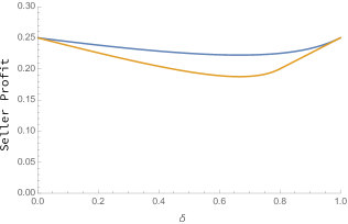
Figure 1: Comparison of seller profit between equilibrium of the baseline model vs. Theorem 2, for Example 1

The proof of the proposition essentially generalizes the example to any setting where the market does not clear at time 2. The key point is that the solution to the baseline model leaves additional scope to transfer surplus to the buyer in order to induce additional delay. In the information structure nature chooses, the seller obtains the exact same continuation profit as in the baseline model, but the inefficiency entailed disappears. Instead, the buyer obtains more surplus, which makes them more willing to delay, thus hurting the seller’s profit.

This result suggests that perhaps the solution to the previous model is not a “true worst-case.” However, one criticism of the benchmark where nature has full commitment is that it requires extreme confidence from the seller regarding nature’s choice of information structure. It seems reasonable to ask where this confidence would come from.

To analyze this question, we consider the following criterion on price paths:

Definition 3.

An optimal pricing strategy from the baseline model is a reinforcing solution if the seller’s anticipated equilibrium profit is equal to the worst-case profit guarantee over the set of all dynamic information arrival processes.

We are not aware of any similar concept being studied elsewhere in the robust mechanism design literature, though we view it as very natural. To maintain focus, we only define reinforcing solutions for the model at hand, though it seems straightforward to extend this to other robust objectives in dynamic settings with limited commitment. This definition could reflect, for instance, some misspecification about the commitment power of nature, with the seller believing information to be sequentially worst-case, whether or not it actually is. One can then ask how much (expected discounted) profit the seller is guaranteed when information can be arbitrary. In a reinforcing solution, even if nature could commit to arbitrary information arrival processes, this extra commitment cannot hurt the seller. The seller’s payoff would be unchanged.

In our exercise, we find reinforcing solutions intuitively appealing as the solution to the following exercise:

• A seller chooses a model of how buyers learn about their values, doing so in an optimistic way in order to maximize their own profits.

• Upon making this choice, however, the seller becomes pessimistic and reconsiders; the worry is that perhaps they were wrong, and they also lack confidence in their understanding of the environment. The seller abandons a model if there were some information arrival process the buyer could have which would deliver lower expected profit.

A reinforcing solution—and in particular, the one we highlight—resolves the “optimism–pessimism” tradeoff highlighted by this thought experiment. An optimistic seller may assume an information structure that delivers high profits, but would reconsider this given their lack of understanding of the environment. By contrast, an overly pessimistic seller may doubt their reasons for being so pessimistic. If a price path satisfies the reinforcing criterion, a seller may think that they might as well use it, and can then rest assured that their profit guarantee would not change if in fact they were wrong—no matter how pessimistic they are.

The condition we need for the solution we highlighted to be a reinforcing one is the following:

Definition 4.

We say that a distribution $F$ satisfies pressed-ratio monotonicity if $\frac{v}{F^{-1}(G(v))}$ is weakly decreasing in $v$.

This assumption is satisfied for many distributions (for instance, all uniform distributions). Intuitively, the definition rules out cases where too much mass is located at the top of the distribution (see also Proposition 4). In this case, a small increase threshold used in order to induce the buyer to delay leads to a larger change in the expectation of $\mathbb{E}[v\mid v\leq y]$.

Under the assumption of pressed-ratio monotonicity, we can show the following:

Theorem 2.

Suppose the value distribution satisfies pressed-ratio monotonicity. Then the equilibrium outcome in Theorem 1 is a reinforcing solution—that is, if the seller uses the outlined strategy, then there is no information arrival process which leads to lower expected payoff for the seller.

The Theorem explicitly solves for nature’s information structure under the assumption of pressed-ratio monotonicity, and shows that this involves the same information structure choice as in Theorem 1. The first step to prove this theorem is to note that the worst-case information structure is partitional. One may expect that this means the result is immediate; however, this is incorrect, as Libgober and Mu (2021) showed via example that this property does not imply the worst-case information structure is the one identified in Theorem 1. That is, nature’s optimal choice of information structure against a given price path may involve the buyer strictly preferring to delay purchase. Even when restricting to partitional information structures, nature’s optimization problem still involves a non-trivial choice of a threshold for each time period, subject to satisfying the obedience conditions of the buyer.

We get around this issue by identifying a particular adjustment of the partition thresholds which leads to a decrease in profit whenever some threshold does not induce exact indifference when given the recommendation to not buy. While lowering the threshold induces more sale in that period, we require nature to adjust the previous period’s threshold so that the buyer’s indifference condition is maintained. In the Appendix, we verify that under pressed-ratio monotonicity, this will always lead to a loss of profit for the seller.

While the pressed-ratio monotonicity condition appears restrictive, we note that it will always hold in some neighborhood of the lower bound of the value distribution:

Proposition 4.

For any continuous distribution $v\sim f$ in the gap case, there exists some $y^{*}>\underline{v}$ such that the distribution of $v$ conditional on being less than $y^{*}$ satisfies pressed-ratio monotonicity.

As a corollary of this proposition, all equilibria are reinforcing solutions if the initial threshold is sufficiently close to $\underline{v}$. Alternatively, the equilibria are eventually reinforcing (i.e., after sufficiently many periods) if the threshold values approach $\underline{v}$, which happens whenever price discrimination becomes sufficiently fine in the limit as $\delta\rightarrow 1$.

he No-Gap Case

Our analysis so far has assumed that $\underline{v}>0$, which past work has shown is a key assumption to deliver the Coase conjecture under known values. We note that, in the case of a finite horizon, identical results apply to the no-gap case as well. However, with an infinite horizon, the story is different. On the one hand, Ausubel and Deneckere (1989) show that in the no-gap case, an equilibrium exists ensuring that the monopolist obtains arbitrarily low levels of profit as the time between offers shrinks to 0. Though trade does not occur with probability 1 by any finite time, this equilibrium is otherwise Coasian, as the market anticipates that the monopolist will cannibalize future demand. Using this equilibrium, however, they derive a folk theorem which ensures that the monopolist obtains a profit level very close to what would be obtained under commitment. The idea is simple: A monopolist is deterred from lowering prices too much, at every point in time, via a punishment which reverts to the Coasian equilibrium where profit levels are arbitrarily low.

The lack of a gap does not prevent the stationary equilibrium we identified from being an equilibrium. Intuitively, this follows from continuity taking $T\rightarrow\infty$, as the proof of Theorem 1 did not assume a gap. On the other hand, we should not expect a uniqueness result to obtain here, since one does not obtain under known-values, and so the question is whether there are equilibria in our baseline game which do not resemble any known-values equilibrium. In fact, since the folk theorem of Ausubel and Deneckere (1989) shows a range of possible outcomes for the seller, we can use their constructions to not only discipline the behavior of the seller, but nature as well.

Using this, we can show that not only does multiplicity enable the possibility of indeterminacy in the seller’s payoff, but also that the corresponding outcome may be qualitatively different from any known-values equilibrium, dramatically breaking the analogy between the two settings.

Proposition 5.

Suppose $\underline{v}=0$, and that the distributions $F$ and $G$ satisfy Definition 5.1 of Ausubel and Deneckere (1989). Then the information structure from Proposition 2 can emerge as an equilibrium outcome.

The proposition is noteworthy because not only does it demonstrate that in the gap case we may have a failure of the Coase conjecture, but also a failure of the analogy to known-values. The equilibrium described in Proposition 2 is unlike any that emerge without the buyer learning over time (e.g., under known-values), since (a) the buyer obtains zero surplus and yet (b) the market never clears. It is worth noting that subtleties such as these fail to emerge in the commitment case. There, the uniqueness is much more immediate, since the seller essentially faces a decision problem, only taking an action once before anyone else. However, the fact that the limited commitment setting is necessarily a game means such uniqueness can no longer be taken for granted; and indeed, once uniqueness fails, so too might the analogy to known values.

If the equilibrium selection were chosen to minimize the seller’s profit, then these issues would not arise and the equilibrium would still feature Coasian dynamics. Nevertheless, it is worth noting that in our setting, whether the equilibrium is chosen to minimize or maximize the seller’s profit plays a role, as static settings (where some form of the minmax theorem typically holds) do not feature such dramatic discontinuities (see Brooks and Du (2020)).

ther Maxmin Benchmarks?

While we hope the analysis in this paper will be useful more generally, as we exposited our model in terms of the behavior of a decisionmaker who plays a game against nature, it is perhaps helpful to clarify exactly the set of possible assumptions we could have made. In doing so, we hope to deliver some appreciation regarding of our main benchmark, while also clarifying the challenges which may emerge in future work.

Despite our focus, we only advocate that the solution concept in Definition 1 is most meaningful in our setting. We are agnostic about this more generally. The assumption was useful here due to the analogy to the known values outcome obtained via appealing to the pressed distribution. In this section, we articulate some alternative benchmarks, and describe why these are less compelling in the informationally robust dynamic durable goods setting. But in other applications, such analogies may not be natural, alternatives may be more tractable, naiveté might be economically justifiable, and so on. Thus, it is worth clarifying what some alternative approaches could be.

Fully articulating each benchmark formally would take us too far afield; instead, we use examples or simplifications to clarify why each one would have influenced the analysis, thus providing intuition for what the impact of our modelling choices were. Throughout this section, we focus again exclusively on the gap case, otherwise we fully maintain the basic structure of the game we analyze; therefore, Sections 2.1, 2.2 and 2.3 should be understood as applying in their entirety. Instead, we will consider alternative solution notions different from Definition 1.

6.1 Naiveté over Future Actions

In Section 2, we showed that there generally exists an information arrival process and equilibrium under which the seller’s profit is lower than in the main model. Therefore, considering the worst case over the “set of all possible information arrival processes and equilibria” requires the seller to no longer choose a maxmin optimal price at time 2.

An alternative way to approach this, however, would be to insist that the seller does consider the worst-case over all information arrival processes, but does not realize that this worst-case will change over time, and correspondingly, does not realize that his future choices will be different. This amounts to changing both (a) the “Bayesian updating whenever possible” requirement, and (b) the requirement that information is sequentially-worst case; that is, in considering the worst-case information arrival process, the seller anticipates choosing an action in the future which he does not realize he would not actually choose were the opportunity to arise.

Specifically, suppose the seller chooses the prices as follows:

• At time $t$, the seller observes all choices of nature and the buyer at time $t=1,2,\ldots$.

• The seller then chooses a price $p_{t}$ subject to the condition of maximizing profit against all possible information arrival processes, and sequential equilibria (i.e., seller pricing strategies and buyer purchasing strategies) under any particular information arrival processes.

In this formulation, the seller displays naivité, in the sense that he simply expects himself to take certain actions in the future, and considers a worst-case with respect to those actions, failing to realize that such actions would not be worst-case in the future. The fact that this may not be a sensible model for a “sufficiently introspective” seller is immediate, since calculating the optimal action in the future would reveal that these are not maxmin optimal.

In fact, the following example illustrates a more dramatic peculiarity:

Example 2.

Take $T=\infty$ and (as with Example 1) $v\sim U[0,2]$, so that the pressed distribution is $U[0,1]$. For fixed $\delta$, the solution in the Coasian equilibrium in the known values case with $v\sim U[0,1]$ is present in Gul et al. (1986) and Stokey (1981) (reviewed in Ausubel et al. (2002)); while other equilibria exist, we have note that the unique outcome for a fixed $\delta$ with $v\sim U[\varepsilon,1]$ converges to this solution as $\varepsilon\rightarrow 0$, and for our purposes the same point would remain by considering a sufficiently small $\varepsilon$. In the known-values case with $v\sim U[0,1]$, the seller’s profit when $\tilde{v}$ is the highest buyer value remaining is given by:

$$\pi^{*}(\tilde{v})=\frac{1}{2}\left(1-\frac{1}{\delta}+\frac{1}{\delta}\sqrt{1-\delta}\right)\tilde{v}^{2}$$

One can verify that $\lim_{\delta\rightarrow 1}\pi^{*}(1)=0$, as predicted by the Coase conjecture. Note that, as above, the worst-case information structure in the first period is partitional, and induces trade with probability 1 in the second period, using the same argument as in example 1.

What does this yield for a seller that is fully-maxmin and naive about his future actions? Suppose the information structure informs the buyer whether or not $v$ is above or below $v^{*}$. A buyer will be made indifferent between delaying and not if:

$$\frac{v^{*}}{2}-p_{1}=\delta\left(\frac{v^{*}}{2}-\pi^{*}(v^{*}/2)\right);$$

In particular, the seller’s profit when the buyer knows $v<v^{*}$ coincides with the profit under known values, truncated at $v^{*}/2$.

Assume for the moment that this equality were to hold. In this case, the seller’s problem could be written as optimizing over the choice of $v^{*}$ instead of $p_{1}$, yielding seller profit as:

$$\frac{v^{*}}{8}(4(1-\delta)-v^{*}(1-\delta-\sqrt{1-\delta}))(1-\frac{v^{*}}{2})+\delta\pi^{*}(\tilde{v}/2).$$

Optimizing over $v^{*}$ (using the formula for $\pi^{*}(\tilde{v})$) gives a solution; however, note that a constraint is that $v^{*}\leq 2$. One can check that this constraint does not bind if and only if $\delta\leq 8/9$. If $\delta>8/9$, it follows that trade does not occur in the first period.

This example is similar to Example 1, where, when $\delta\geq 4/5$, trade does not occur in the first period. The only difference is that now the horizon is infinite. As a result, the seller’s problem at time 2 looks identical to the time 1, whenever sale occurs with probability 0 at time 1.

So suppose the seller were to consider the true worst-case information arrival process, being naive over future actions. In this case, the seller would never induce a sale. After waiting one period, the seller would “reset” the worst-case. As this behavior does not emerge in any Bayesian Coase conjecture environment (where the seller at least tries to sell), we note that despite doing even worse than the Coase conjecture presents, the resulting equilibrium is non-Coasian.

While the above behavior appears suspicious, we view this as an indictment of the model of the fully-pessimal-and-naive benchmark. It seems hard to imagine that the seller, capable of computing their discounted payoffs, would not further realize their strategy would involve “never-selling.” Indeed, if $\underline{v}>0$, then the seller can always choose some price where every buyer would wish to buy, for any value of $v$. A seller realizing this might instead opt to adopt such a safe strategy instead of following the predictions of this benchmark.

6.2 Sophistication

While the previous section shows that the worst-case information structure for the seller at $t=1$ will generally induce an equilibrium where the seller does not optimize against the worst-case at time $t=2$, one might instead insist on maintaining that the seller maximizes against the worst-case information arrival process, but acknowledges that this may change over time. Such a seller is dynamically inconsistent, but aware of this.

To be precise, this alternative induces the following assumption regarding the objectives of each of the players is as follows:

• At time 1, the seller anticipates the choice $p_{2}(p_{1})$ that he would make at time 2, and chooses the price $p_{1}$ to maximize profit against the worst-case information arrival process, given $p_{1}$ and $p_{2}(p_{1})$.

• Nature then chooses an information structure, $\mathcal{I}_{1}$ for the buyer, to minimize the seller’s total discounted profit at time 1, assuming the worst-case choice of $\mathcal{I}_{2}$ given $p_{2}(p_{1})$. The choice of $\mathcal{I}_{1}$ is observed by the time 2 seller (and the buyer).

• At time 1, the buyer decides whether to purchase or not as a function of the worst-case information arrival process the seller expects at time 1.

• At time 2, the seller maximizes profit assuming the worst case information structure at time 2, holding fixed $\mathcal{I}_{1}$. This determines $p_{2}(p_{1})$.

• At time 2, the buyer decides whether to purchase depending on whether or not his expected value is above the price, breaking indifference against the seller.

This model is substantially more complicated than the benchmark model, because it requires us to solve for an information arrival process at every time the seller acts. Rather than solving a single information design problem, as in our benchmark model, this version requires us to solve as many information design problems as time periods, and for the seller to optimize over all of these.

We make two comments on this alternative. First, this alternative benchmark provides a new way of interpreting Theorem 2: Under pressed-ratio monotonicity, the price path chosen by a sophisticated maxmin seller will coincide with the price path from the main model. The reason is simple: The full worst-case information structure in the second bulletpoint always coincides with the no-commitment worst case. Under pressed-ratio monotonicity, a dynamically consistent and correct seller is also “sophisticated and fully-worst-case.”

In general, however, the sophisticated benchmark differs from the one in this model. We present an example of this in the appendix, and one that features discrete values, where the worst-case information structure is not the one necessary to induce the outcome described in Theorem 1. We are not able to say much more than this. Solving for the equilibrium price paths for this alternative, even in simple examples, is beyond the scope of our existing techniques we are aware of, and thus for now we leave it as an open problem. While we expect the resulting price paths to be qualitatively similar, for our purposes the key point is the following: the resulting equilibrium can be interpreted as displaying non-Coasian forces, since both our model and this alternative induce identical single-period problems (and importantly, same corresponding “as-if known values” distribution), but different dynamic solutions. Thus, insofar as the analogy to the known-values case is an aesthetically appealing property of our main benchmark, it is worth noting that this alternative does not necessarily induce equilibria where this analogy is meaningful.

6.3 Worse Past Information

We have assumed that the seller posits all past actions of nature as “sunk.” Since we assume that the choices of nature are observed, the seller who chooses a price at time $t$ does not consider the worst-case information structure at time $s<t$—that is, this information structure is assumed to be known. However, without this observability assumption, it becomes necessary to consider the worst-case over past information as well.

Specifically, assume the following, and for simplicity take $T=2$.

• At time 1, the timing protocol is exactly as in the main model.

• At time 2, the seller chooses a price to maximize the profit guarantee, taken over all $\mathcal{I}_{1},\mathcal{I}_{2}$, and conditional on the buyer not having purchased at time 1.

To obtain a coherent statement while avoiding conceptual difficulties, in the following proposition, we treat the buyer as a completely passive player and do not consider their incentives, taking $\hat{p}_{2}(p_{1})$ as a primitive. This allows us to focus on the solution to nature’s problem at time $T=2$, when its choice is over the buyer’s information at both times 1 and 2:

Proposition 6.

Suppose $T=2$, and suppose that the seller seeks to maximize the profit guarantee at time $2$ over both the information in both periods. Suppose that, at time 2, the seller conjectures that the buyer conjectured the second period price to be $\hat{p}_{2}(p_{1})$ (or, more generally, a random variable with mean $\hat{p}_{2}(p_{1}))$. Let $v^{*}=\frac{p_{1}-\delta\hat{p}_{2}(p_{1})}{1-\delta}$, and suppose that $v^{*}>\mathbb{E}_{F}[v]$. Then given a price of $p_{1}$, the worst-case information structure in period 1 is characterized by a threshold $y^{*}$ where the buyer learns whether $v>y^{*}$ or not, and $y^{*}$ is either equal to $\underline{v}$ or characterized by:

$$\mathbb{E}[v\mid v>y^{*}]=\frac{p_{1}-\delta\hat{p}_{2}(p_{1})}{1-\delta}.$$

Thus, the indifference condition that pins down the period 1 threshold changes from inducing the lowest probability of sale (as shown in Section 3) to the highest probability of sale. Intuitively, this is because nature can, in this alternative, condition on the fact that the buyer has not bought when choosing the information structure at time 1. This is still restricted, since the buyer would need to have been willing to purchase given the conjecture. However, choosing the information in this way suggests that the buyers who remain are the lowest possible value. Thus, if nature can also optimize over past information, the solution would entail past information having been chosen as favorably as possible—intuitively, because then all remaining buyers are less favorable.

There are two reasons we stop short of a full characterization of equilibrium. First, to do this formally requires more details than the above description provides, since one needs to specify how the seller resolves his time inconsistency, in addition to how the seller believes the buyer believes the seller resolves his time inconsistency. At time 1, the problem appears to the seller exactly as in the baseline model, but at time 2 the problem seems very different; thus we have (at least) two possible candidates for $\hat{p}_{2}(p_{1})$, and so without an assumption on (the seller’s belief of) buyer equilibrium behavior, we cannot specify which first-period indifference threshold is relevant.

Second, characterizing the full equilibrium would require us to drop the assumption that $v^{*}>\mathbb{E}_{F}[v]$, since this is an assumption on endogenous objects. The problem is that without this assumption, the seller would think the buyer should have bought at time 1 with probability 1. The seller would then believe himself at a probability 0 event whenever the game continues to time 2. While one could discipline beliefs here in various ways, we do not wish to take a stand on this.

In any case, added conceptual difficulties aside, Proposition 6 clarifies the kind of dynamic inconsistency issues that emerge if the seller also considers the worst-case over past information. This alternative seems suspicious, as it suggests the seller always believes the past information was chosen favorably while future information was chosen unfavorably. We leave our analysis of this alternative to this observation.

onclusion

In this paper, we propose a new approach to modelling a designer who has limited commitment and (re)optimizes a dynamic worst-case objective. By treating the adversarial nature as another player in the dynamic game, we obtain a dynamically consistent worst-case objective for the designer. We feel that our particular setting of durable goods sales is a natural laboratory for this exercise, for two reasons: First, there is a vast literature on the Coase conjecture, so in our analysis we can often appeal to the known forces that drive equilibria in this setting. Second, the need to accommodate information arrival into durable goods pricing has already been recognized by the literature, and in this paper we fill this gap with our proposed dynamic robust approach.

In the context of durable goods pricing, the main takeaway of the paper is that when a seller is aware of the possibility of buyer learning but uncertain about it, he should nonetheless set prices as if the buyer knew her value to begin with (thus no learning). This analogy, between our unknown-values environment and the classic known values environment, holds so long as the seller applies a suitable transformation to the buyer’s value distribution to take into account his robust objective. As we discussed in the paper, Coasian dynamics often fail under alternative models of buyer learning. Thus we are able to restore the Coase conjecture using a robust approach.

Going beyond our particular setting, we hope that the paper has provided a template that can be used to extend the reach of the robust approach to dynamic interactions. The “as-if known values” solution in Theorem 1 illustrates that equilibrium can be fairly tractable if the seller is only concerned about dynamically-consistent information processes. While one may argue that focusing on this restricted worst-case is at odds with the robust objective, we also showed that this criticism often turns out to have no bite in our setting. By introducing the notion of a reinforcing solution, we hope that other researchers will be able to derive tractable solutions to similar dynamic robustness models, and plausibly argue that such solutions do not compromise the motivation for adopting the robust approach in the first place.

Appendix A Proofs for Section 3

Proof of Theorem 1.

To analyze this game, we first note that the buyer’s problem is relatively simple. Since the buyer’s decision has no effect on future prices and information (which are anyways conditional on her not purchasing), she faces an optimal stopping problem given any history.

Using the fact that we have a finite horizon, we can then turn to nature’s problem and apply backwards induction. In the final period, given $(p_{t})_{t=1}^{T-1},(\mathcal{I}_{t})_{t=1}^{T-1}$, nature chooses an information structure $\mathcal{I}_{T}:V\times S^{T-1}\to\Delta(S_{T})$ to minimize the seller’s profit. Our first goal below is to show that $\mathcal{I}_{T}$ can be taken to be the worst-case threshold information structure for $p_{2}$, without affecting the equilibrium outcome.

Let $s=(s_{1},\ldots,s_{T-1})$ be a generic signal history up until time $T$. Each signal history induces a posterior distribution of $v$, denoted $F_{s}$. First suppose $s$ is such that the buyer does not purchase before the final period, according to the equilibrium strategy (given the price history and history of information structure, as well as the expectations of the final period prices and information). Then sequential rationality requires nature to minimize profit from this buyer type in the final period, implying that $\mathcal{I}_{T}(s)$ must be a worst-case information structure for the distribution $F_{s}$ and price $p_{T}$. Denote the minimum value in $F_{s}$ by $\underline{v}_{s}$, and its expected value by $\mathbb{E}[F_{s}]$. There are three cases:

1. If $p_{T}<\underline{v}_{s}$ or $p_{T}>\mathbb{E}[F_{s}]$, nature’s problem is trivial and it is without loss to assume nature provides no information in period $T$.

2. If $p_{T}\in(\underline{v}_{s},~{}\mathbb{E}[F_{s}]]$, then for each $\epsilon>0$, nature could reveal the worst-case threshold for $p_{T}-\epsilon$. This would lead to profit $p_{T}\cdot(1-G_{s}(p_{T}-\epsilon))$ in period $T$, so equilibrium profit must be bounded above by $p_{T}\cdot(1-G_{s}(p_{T}))$ by taking $\epsilon\to 0$ (note that $G$ is continuous at $p_{T}$ when $p_{T}>\underline{v}_{s}$). On the other hand, we know that equilibrium profit cannot be lower regardless of what nature and buyer do. Hence we can without loss assume that nature provides the worst-case threshold information structure for $p_{T}$, and that the buyer breaks indifference against the seller.

3. The remaining possibility is $p_{T}=\underline{v}_{s}$. If $F_{s}$ does not have a mass point at its lowest value, then the same argument applies since $G_{s}$ is still continuous at $p_{T}$. But if $F_{s}$ has a mass point of $m=G_{s}(p_{T})$ at $p_{T}$, then any profit level in the interval $[p_{T}(1-m),~{}p_{T}]$ may be supported in equilibrium, depending on how the buyer breaks ties. In this case it is without loss to assume that nature reveals whether $v=p_{T}$ or not, and that the buyer breaks indifference in some way. Note that in this case, the seller’s profit is hemicontinuous in $p_{T}$; as there is a set of possible profit levels at $p_{T}=\underline{v}_{s}$, and a unique (and continuous) profit level at $p_{T}<\underline{v}_{s}$ and $p_{T}>\underline{v}_{s}$.

Suppose instead that the signal realization $s$ is such that the buyer purchases before the final period. In this case, we may assume nature uses the worst-case threshold information structure in the last period, which minimizes the buyer’s option value (since the buyer is made indifferent between purchasing and not according to this information structure), and ensures that the buyer still purchases before the final period.

We now suppose that we have shown that nature will use a partitional information structure for all periods after the first period. We now turn to nature’s decision in period 1, showing that nature will again seek to do this in the first period. Given any price $p_{1}$ in period 1, nature expects the possibly random price $p_{2}=\hat{p}_{2}(p_{1})$ in period 2. Define the binding cutoffs $w_{1},w_{2}$ by

$$w_{1}-p_{1} =\delta\cdot\mathbb{E}\left[(w_{1}-p_{2})^{+}\right];$$

$$w_{2} =\min\{w_{1},p_{2}\}.$$

First note that given the previous analysis, nature’s information choice in period 2 leaves the buyer with the same surplus as if no information were provided in that period. Knowing this, the buyer’s purchase decision in period 1 depends entirely on whether $\mathbb{E}[F_{s_{1}}]$ is bigger or smaller than $w_{1}$. For now, ties may be broken arbitrarily when indifferent, although we will see shortly that equilibrium requires breaking ties against the seller.

Note that, by assumption, the prior distribution $F$ is continuous, and therefore does not have a mass point at its lowest value. We will show that nature’s choice of $\mathcal{I}_{1}$ must be outcome-equivalent to the worst-case threshold information structure for $w_{1}$, and that the buyer must break indifference against the seller. On the one hand, for each $\epsilon>0$ nature could provide the threshold information structure for $w_{1}-\epsilon$. Given what happens in period 2, and taking $\epsilon$ sufficiently small so that this does not influence the decision at any time after the second period, this would lead to total profit

$$p_{1}(1-G(w_{1}-\epsilon))+\delta\cdot\mathbb{E}[p_{2}\cdot(G(w_{1}-\epsilon)-G(w_{2}))^{+}]+\sum_{s=0}^{T-2}\delta^{2}p_{s+2}\mathbb{E}[p_{s+2}\cdot(G(w_{s+1})-G(w_{s+2})^{+})]$$

Letting $\epsilon\to 0$, we know that equilibrium profit following the price $p_{1}$ satisfies (taking the convention that $G(w_{0})=1$:

$$\Pi\leq\sum_{t=0}^{T}p_{t+1}\delta^{t}\mathbb{E}[p_{t}(G(w_{t})-G(w_{t+1}))].$$

On the other hand, we will show that the right hand side of this expression is also a lower bound for profit, for any choice of $\mathcal{I}_{1}$ and any tie-breaking rule. Indeed, if $w_{1}\leq\underline{v}$ then every type of the buyer purchases in period 1, and the result holds. Suppose $w_{1}>\underline{v}$, we first show that every realization of $p_{2}$ satisfies $p_{2}\leq w_{1}$. Recall that in period 2, any buyer who remains has expected value at most $w_{1}$. Knowing this, a price greater than $w_{1}$ leads to zero profit for the seller in period 2. This can only be optimal if the seller expects nature’s equilibrium choice of $\hat{\mathcal{I}}_{1}$ to clear the market in period 1. We claim that this cannot occur in equilibrium. Indeed, instead of making everybody purchase, nature could reveal whether $v\in[\underline{v},w_{1})$, making this interval of buyers delay until period 2. The effect on profit is a loss of $p_{1}$ in period 1, and a gain of at most $\delta\cdot\mathbb{P}(p_{2}<w_{1})\cdot\mathbb{E}[p_{2}\mid p_{2}<w_{1}]$ in period 2, since these buyers purchase at $p_{2}$ only if $p_{2}<w_{1}$. From the definition of $w_{1}$ above, we have

$$w_{1}-p_{1}=\delta\cdot\mathbb{P}(p_{2}<w_{1})\cdot\mathbb{E}[w_{1}-p_{2}\mid p_{2}<w_{1}].$$

Rearranging yields $p_{1}-\delta\cdot\mathbb{P}(p_{2}<w_{1})\cdot\mathbb{E}[p_{2}\mid p_{2}<w_{1}]=w_{1}-\delta\cdot\mathbb{P}(p_{2}<w_{1})\cdot w_{1}>0$. Hence this deviation would lower the seller’s profit.

Now that we know $p_{2}\leq w_{1}$ almost surely, the definition of $w_{1}$ further gives $w_{1}-p_{1}=\delta\cdot\mathbb{E}[w_{1}-p_{2}]$. It follows that

$$p_{1}>\delta\cdot\mathbb{E}[p_{2}],$$

which will be useful below.

We claim that in order to minimize the seller’s profit, the buyer should break ties against the seller. Indeed, the effect of delay on profit is a loss of $p_{1}$ in period 1, and a gain of at most $\delta\cdot\mathbb{E}[p_{2}]$ in period 2, resulting in a net decrease in profit. Next, it is without to assume nature provides only two signal realizations $\overline{s}_{1}$ and $\underline{s}_{1}$, which lead to buyer expected values $>w_{1}$ and $\leq w_{1}$, respectively. This is because any extra information in period 1 that does not change the buyer’s action can be deferred to period 2. Moreover, $\underline{s}_{1}$ occurs with positive probability, since otherwise the market is cleared in period 1, in which case nature could deviate to lower the seller’s profit as shown above.

Additionally, if $\overline{s}_{1}$ also occurs with positive probability, then $\underline{s}_{1}$ must lead to expected value exactly $w_{1}$. Otherwise, nature could mix a small fraction of $\overline{s}_{1}$ with $\underline{s}_{1}$, making this fraction of $\overline{s}_{1}$ no longer purchase in period 1. Suppose also that in period 2 nature separates this fraction of $\overline{s}_{1}$ from the $\underline{s}_{1}$ buyers and reveal the worst-case threshold for each group (which may not be optimal in period 2, but allows for easy comparison of profit). Then even if the fraction of $\overline{s}_{1}$ buyers always purchases in period 2, the profit gain is bounded above by $\delta\cdot\mathbb{E}[p_{2}]$. This is less than $p_{1}$, proving that the deviation would be profitable.

We can now show that the seller’s profit is minimized when nature reveals the worst-case threshold for $w_{1}$ (and the buyer breaks indifference against the seller). If $w_{1}\geq\mathbb{E}[v]$, then whenever $\overline{s}_{1}$ occurs the other signal $\underline{s}_{1}$ must lead to expected value less than $w_{1}$. This contradicts optimality as shown above. Thus in this case nature optimally only provides a single signal $\underline{s}_{1}$, corresponding to no information.

If instead $w_{1}<\mathbb{E}[v]$, then $\overline{s}_{1}$ must occur with positive probability. So $\underline{s}_{1}$ leads to expected value exactly $w_{1}$. We claim that $\underline{s}_{1}$ must correspond to all the buyer types below the worst-case threshold for $w_{1}$. Suppose this is not the case, then we can find $v^{\prime}$ in the support of $F_{\underline{s}_{1}}$ and $v^{\prime\prime}$ in the support of $F_{\overline{s}_{1}}$ such that $v^{\prime}>v^{\prime\prime}$. If nature were to “swap” $v^{\prime}$ and $v^{\prime\prime}$ with small probability, then the expected value following the modified $\overline{s}_{1}$ would still exceed $w_{1}$, leading to the same buyer action. Moreover, the entire posterior distribution following the modified $\underline{s}_{1}$ is shifted down in the FOSD sense, so profit is weakly decreased. Now since the expected value following the modified $\underline{s}_{1}$ is strictly less than $w_{1}$, there is room for further reducing the profit as described above. Hence the desired contradiction.

In fact, we know from this analysis that in equilibrium, nature must minimize the probability of purchase at $w_{1}$, and the buyer must break indifference against the seller. We are not done, however, since in period 1 nature could potentially provide more information than the worst-case threshold (for example making the buyer’s posterior distribution supported on only two values). This would affect the seller’s belief about the buyer’s value distribution in period 2, and influence the optimal price $p_{2}$.

To address this issue, we are going to show that the price $p_{2}$ would remain optimal if nature were to simply provide the worst-case threshold information structure for $w_{1}$ in period 1. To this end, note that in this equilibrium, any realization of $p_{2}$ must be maxmin optimal against a buyer who knows her value to be in the lowest $G(w_{1})$-percentile and potentially knows more. Moreover, as calculated above, the maxmin optimal profit in period 2 must be $p_{2}(G(w_{1})-G(w_{2}))$ (which must be the same number for all realizations of $p_{2}$). Now, against a less informed buyer who only knows her value to be below the $G(w_{1})$-percentile, the maximal optimal profit can only decrease. But charging price $p_{2}$ against such a buyer guarantees $p_{2}(G(w_{1})-G(w_{2}))$, so it remains the seller’s best response.

Hence, we have shown that every equilibrium is outcome-equivalent to an equilibrium in which nature provides threshold information structures, where the threshold is chosen so that conditional on having value below the threshold, the buyer is indifferent between purchasing in the current period or delaying until the future (without further information). Moreover, the seller thinks the buyer always breaks indifference against him (even though this is not necessarily true in period 2, if nature has deviated in period 1). Therefore, given any equilibrium price path shaping expectations, the seller’s probability of sale in each period under any deviation strategy is the same as the known-values case, with $G$ replacing $F$ as the value distribution. It follows that any equilibrium in our model is equivalent to an equilibrium in the known-values case with the transformed value distribution $G$. ∎

Proof of Proposition 1.

Suppose the seller chooses price $p_{1}$ in period 1, and suppose a candidate equilibrium required nature to choose information structure $\mathcal{I}_{1}$. To deter a deviation from nature, we suppose that the continuation play following nature’s deviation is as good as possible from the seller. Therefore, if $(\hat{p}_{2},\hat{p}_{3},\ldots,)$ is the conjectured price path the buyer would imagine the seller would use, following this deviation, then we can define $\hat{w}(p_{1})$ to be the expected value of the buyer which would be indifferent between buying and not, assuming no further information:

$$\hat{w}(p_{1})-p_{1}=\max_{\tau}\delta^{\tau}(\hat{w}(p_{1})-\hat{p}_{\tau})$$

Note that if the buyer were to receive information in future periods, then this would make delay more attractive, therefore making the buyer strictly prefer delay to purchase. On the other hand, since $p_{1}>\delta\mathbb{E}[p_{2}]$ in any equilibrium (as argued in the Proof of Theorem 1).

So, let $w^{*}(p_{1})=\inf_{(\hat{p}_{2},\hat{p}_{3},\ldots)}\hat{w}(p_{1})$. Consider deviations of nature from $\mathcal{I}_{1}$ where the buyer is told whether $v$ is above or below $F^{-1}(G(w^{*}(p_{1})))-\varepsilon$, for $\varepsilon\rightarrow 0$. Then if $v$ is below this threshold, there is no conjecture the buyer could make about the seller’s future behavior which would lead them to want to purchase, by the definition of $w^{*}(p_{1})$. On the other hand, above this threshold, for $\varepsilon$ small, we will have $\mathbb{E}[v\mid v\geq F^{-1}(G(w^{*}(p_{1})))-\varepsilon]>w^{*}(p_{1})$ and therefore the buyer will buy, given this conjecture.

So, by deviating in this way, nature has the ability to ensure the seller only obtains $p_{1}(1-G(w^{*}(p_{1})))$ in period 1. With this in mind, let $\overline{v}_{t}$ be the highest consumer value that has not purchased by time $t$, and $\overline{y}(p_{1})$ thecorresponding choice of nature. We then have the following recursive formulation for an upper bound of the seller’s profit, for every $p_{1}$:

$$V(\overline{v}_{t})=p_{1}(1-G(w^{*}(p_{1})))+\delta V(\overline{y}(p_{1}))$$

This is precisely the value function in the known values case of Theorem 4 of Ausubel et al. (2002), when the buyer’s value is distributed according to $G$. While we emphasize that the above expression has a less direct interpretation—namely, as an upper bound on the equilibrium profit—nevertheless the result immediately implies that the equilibrium values of $V_{t}$ must be equal to $\overline{v}$ at some $t$.

Therefore, the following pair of claims will deliver the proposition:

Claim 1: If $V_{t}=\underline{v}$, then the market is cleared in finite time.

Proof of Claim 1: Note that there exists a range of choices of $p$ for the seller, say $[\underline{v},p^{*}]$, such that the seller optimally clears the market in the next period after charging a price of $p$. Indeed, since nature can always choose the threshold $F^{-1}(G(p))$, then there exists a range where, if the seller were to charge a price in this range, nature could ensure this price lead to a total payoff of less than $\underline{v}$ (since this holds under known values). Therefore, were we to have an equilibrium with $V_{t}=\underline{v}$ for infinitely many periods, then we must also have $p_{s}\rightarrow p^{**}$ for some $p^{**}\geq p^{*}$, and the seller obtaining a total discounted payoff of $p_{s}$ under the information structure. On the other hand, for any distribution of expected values of the buyer, the previous proof shows that if the seller chooses the Coasian price path, the worst-case the seller can obtain is strictly larger than $\underline{v}$. Therefore, the seller would have a profitable deviation in any such equilibrium.

Claim 2: If $F$ satisfies the Lipschitz condition of Theorem 4 of Ausubel et al. (2002), then so does $G$.

Proof of Claim 2: Note that, for every quantile $q$, the pressed distribution satisfies $G^{-1}(1-q)<F^{-1}(1-q)$, but the bottom of the support is the same for each. Therefore, we have $G^{-1}(1-q)-\underline{v}<F^{-1}(1-q)-\underline{v}$, so that if $F$ satisfies the Lipschitz condition—i.e., $F^{-1}(q)-\underline{v}\leq Lq$ for all $q$ and some $L$—then so does $G$.

Finishing the proof: Claim 2 shows that the upper bound derived above does indeed ensure that $V_{t}=\underline{v}$ in finite time, since this result holds given any distribution under known values satisfying the Lipschitz condition. Claim 1 therefore shows that, since $V_{t}=\underline{v}$ in every equilibrium, and with an upper bound existing on the number of periods this takes, it therefore follows that there exists an upper bound by which the market has cleared. This shows that in the case of a gap, the infinite horizon game coincides with the outcome of a sufficiently long finite horizon game, completing the proof. ∎

Proof of Proposition 2.

We consider two cases for this proof; in the first case we take $T=\infty$ and in the second case we take $T<\infty$. The idea behind the construction in both cases is the following:

• On-path, the seller seller chooses a price equal to the buyer’s expected value, and no information is provided.

• Meanwhile, the buyer randomizes purchase so that the seller has incentives to follow the equilibrium strategy.

• If the seller deviates, the equilibrium reverts to the worst-case outcome outlined in Theorem 1.

We emphasize that there is no choice of nature to consider, as this is simply exhibiting some information structure where there is no bound on the market clearing time.

We now walk through the details more precisely. Take the strategy exactly as above. We already know that following a deviation, buyer’s strategy forms an equilibrium. Indeed, since the buyer’s purchasing decision does not depend on their value, the on-path distribution of $v$ conditional on not having purchased at time $t$ is simply $F$. Thus, the buyer’s problem is completely unchanged relative to the case considered in Theorem 1. The seller’s continuation strategy following a deviation also forms an equilibrium, by construction. Note that, since we assume the buyer randomizes, note that it is not possible for them to deviate, since all actions occur with positive probability on-path.

Therefore, letting $\pi^{*}(G)$ denote the profit achieved in the equilibrium from Theorem 1, the seller obtains at most $\pi^{*}(G)$ following a deviation. Suppose we seek an equilibrium where the seller’s continuation value is $v$ at every point in time, for $v^{*}>\pi^{*}(G)$. In this case, the buyer purchases with probability $\rho$ at every point in time, where $\rho$ satisfies:

$$v^{*}=\rho\mathbb{E}_{F}[v]+(1-\rho)\delta v^{*}\Rightarrow\rho=\frac{v^{*}(1-\delta)}{\mathbb{E}_{F}[v]-\delta v^{*}},$$

where $\rho\in(0,1)$ whenever $v\in(\pi^{*}(G),\mathbb{E}_{v\sim F}[v]$

Thus, by charging $\mathbb{E}_{F}[v]$, the seller obtains a higher payoff than what they could obtain from deviating. We thus verify the conditions are satisfied in the proposition: First, the seller uses a constant price path. Second, the profit obtains is the arbitrary $v^{*}\in(\pi^{*}(G),\mathbb{E}_{v\sim F}[v])$. And lastly, the market does not clear by any finite time; since $\rho$ is constant, the probability the buyer has not bought at or before time $K$ is $(1-\rho)^{K}>0$.

In the case of a finite horizon, the proof is identical except in the last period, we assume the buyer purchases with probability $v/\mathbb{E}_{F}[v]$; here, we note that the seller’s minmax continuation payoff following a deviation is time dependent, although no matter what the time horizon is it is always strictly bounded away from $\mathbb{E}_{F}[v]$ (indeed, it is always lower than the seller’s static monopoly profit, which is lower than $\mathbb{E}_{F}[v]$). Accommodating this is straightforward and thus omitted. ∎

Appendix B Other Proofs

Details for Example 1. We perform the familiar calculation for the equilibrium price path by backwards induction using this known values distribution, using the fact that the equilibrium is of a threshold form. First, note that given an arbitrary first period indifference threshold $\overline{v}$ under known values, we have the seller’s second period price must maximize $p_{2}(1-\frac{p_{2}}{\overline{v}})$, implying that $p_{2}=\frac{\overline{v}}{2}$. Anticipating this and observing a first period price of $p_{1}$, the buyer is indifferent if:

$$\overline{v}-p_{1}=\delta\left(\overline{v}-\frac{\overline{v}}{2}\right)\Rightarrow\overline{v}=\frac{2p_{1}}{2-\delta}.$$

Therefore, the seller at time 1 choose $p_{1}$ to maximize:

$$p_{1}\left(1-\frac{2p_{1}}{2-\delta}\right)+\delta\frac{p_{1}}{2-\delta}\left(\frac{p_{1}}{2-\delta}\right)\Rightarrow 1-\frac{4p_{1}}{2-\delta}+\frac{\delta 2p_{1}}{(2-\delta)^{2}}=0\Rightarrow p_{1}=\frac{(2-\delta)^{2}}{8-6\delta}.$$

Substituting this in gives that profit is:

$$\frac{(2-\delta)^{2}}{8-6\delta}\left(1-\frac{2-\delta}{4-3\delta}\right)+\delta\frac{(2-\delta)^{2}}{(8-6\delta)^{2}}=\frac{(2-\delta)^{2}}{8-6\delta}\left(1-\frac{2-\delta}{4-3\delta}+\frac{\delta}{8-6\delta}\right)\\ =\frac{(2-\delta)^{2}}{8-6\delta}\left(\frac{4-3\delta}{8-6\delta}\right)=\boxed{\frac{(2-\delta)^{2}}{4(4-3\delta)}}.$$

Now we compute the profit under the information structure specified in Proposition 3. First, recall that $\pi^{*}(\tilde{v})=\frac{\tilde{v}}{8}$. Since $\mathbb{E}[v\mid v<\tilde{v}]=\tilde{v}/2$, the buyer obtains $\frac{3\tilde{v}}{8}$ in the second period. Therefore, the buyer’s continuation value, given $\tilde{v}$, solves:

$$\frac{\tilde{v}}{2}-p_{1}=\delta\frac{3\tilde{v}}{8}\Rightarrow\tilde{v}=\frac{8p_{1}}{4-3\delta}.$$

Suppose that nature, in the first period, tells the buyer whether her value is above or below $\frac{8p_{1}}{4-3\delta}$. Given this information structure (as well as understanding that the seller will follow the equilibrium strategy), the buyer will delay if told her value is below the threshold and not if it is above the threshold. Let us assume for the moment that this solution involves purchase in each period with positive probability, handling the case where this does not occur separately. Since the probability the buyer’s value is above the first period threshold is $1-\frac{4p_{1}}{4-3\delta}$ (since $v\sim U[0,2]$), the seller’s profit can be written:

$$p_{1}\left(1-\frac{4p_{1}}{4-3\delta}\right)+\delta\frac{4p_{1}}{4-3\delta}\frac{p_{1}}{4-3\delta}\Rightarrow 1-\frac{8p_{1}}{4-3\delta}+\frac{8p_{1}\delta}{(4-3\delta)^{2}}=0\Rightarrow p_{1}=\frac{(4-3\delta)^{2}}{32(1-\delta)}.$$

Profit at this price is:

$$\frac{(4-3\delta)^{2}}{32(1-\delta)}\left(1-\frac{4(4-3\delta)}{32(1-\delta)}\right)+\delta\frac{4(4-3\delta)^{2}}{(32(1-\delta))^{2}}=\frac{(4-3\delta)^{2}(32(1-\delta)-4(4-3\delta)+4\delta)}{(32(1-\delta))^{2}}=\boxed{\frac{(4-3\delta)^{2}}{64(1-\delta)}}$$

Unlike with the previous case, however, we need to check that this solution does indeed involve sale at both periods. Given $p_{1}$, we have $\tilde{v}=2$ if:

$$1-\frac{(4-3\delta)^{2}}{32(1-\delta)}=\delta\frac{3}{4}\Rightarrow\delta=4/5.$$

So, if $\delta<4/5$, this scheme involves profit exactly as above. If $\delta\geq 4/5$, all buyers delay to the second period and no sale occurs in the first period, meaning the total profit is $\delta/4$.

Proof of Proposition 3.

Let $p_{1}>p_{2}>\ldots>p_{t^{*}}=\underline{v}$ be a solution to the baseline model, with corresponding thresholds $y_{1}>y_{2}>\cdots>y_{t^{*}}=\underline{v}$. Let $U_{2}$ denote the buyer’s expected continuation surplus in this equilibrium starting at the second period, and let $\Pi_{2}$ denote the seller’s continuation profit. Note that:

$$\int_{\underline{v}}^{y_{2}}wf(w)dw>U_{2}+\Pi_{2},$$

since by assumption the baseline model does not involve the market clearing by time two. The idea is to use the fact that there is inefficiency to transfer additional surplus to the buyer in order to induce additional delay.

We do this by considering the following classes of information structures for nature:

• In period 1, nature chooses a threshold $\tilde{y}_{1}$ as a function of the first period price, the seller charges.

• In the second period, if the seller chooses some fixed $p_{2}=\tilde{\Pi}$, then nature reveals no information to the buyer, and reveals no information to the buyer in the future.

• If the seller uses some other price, nature uses the worst-case descending partitional information structure outlined in the proof of Theorem 1.

We will in particular focus on the case where $\tilde{\Pi}$ is the seller’s continuation profit follow some first period threshold of $y_{1}$, which we denote $\Pi_{2}(y_{1})$. Note that in this case, the seller has a best reply to choose $p_{2}=\Pi_{2}(y_{1})$, since by construction deviating cannot lead to a higher profit (otherwise, there would be some other strategy yielding higher profit in the baseline model).

Now, nature choosing some information structure of this form may induce the seller to choose a price such that the market would clear at time 1 or time 2. However, the seller also had the ability to charge one of these prices in the baseline model, and did not, meaning that this will hurt the seller.

On the other hand, for any other price, we have that the threshold $y_{1}$ such that the buyer is willing to not purchase whenever informed that their value is below the threshold satisfies $y_{1}>F^{-1}(G(p_{1}))$, since, by the previous, their continuation surplus increases. It follows that under this class of information structures, the seller sells less in the first period relative to the case without nature commitment, and obtains the same continuation profit, and therefore obtains lower discounted expected profit, as desired. ∎

Proof of Theorem 2.

We fix an arbitrary declining price path $p_{1},\ldots,p_{t^{*}}$ with $p_{t^{*}}=\underline{v}$. We note that in the gap case, such a $t^{*}$ exists for every equilibrium price path whenever $\delta<1$ under a known value distribution. Therefore, using the previous result, such a $t^{*}$ can be always be found in any equilibrium of the game without nature commitment. Furthermore, by Proposition 3 in Libgober and Mu (2021), the worst-case information structure against an arbitrary declining price path is a threshold process. It follows that nature’s choice of information structure is determined by thresholds $y_{1}>y_{2}>\cdots>y_{t^{*}}=\underline{v}$, with the buyer purchasing at the first time $t$ satisfying $v>y_{t}$.

We first note that the buyer always purchases at or before period $t^{*}$. The theorem will follow from showing that each threshold $y_{t}$ should be as low as possible, for all $t<t^{*}$. For the first part of the proof, we consider any information structure with $y_{1}>y_{2}>\cdots>y_{t^{*}}$; we address the case where equality might hold separately. That is, we show that a buyer who does not purchase at some time $t$ must be indifferent between purchasing and continuing in any worst case information structure. This is immediate for $y_{1}$; In this case, increasing $y_{1}$ while holding all other thresholds fixed simply trades off between sale at time 1 and time 2; so, if $y_{1}$ could be raised without changing the buyer’s incentive conditions, since $p_{1}>\delta p_{2}$, this hurts the seller.

Suppose we have that $y_{t}$ is set so that the buyer is indifferent between purchasing and continuing when given the recommendation to not purchase. This gives us the following indifference condition, given our threshold sequence:

$$\int_{\underline{v}}^{y_{t}}(v-p_{t})f(v)dv=\sum_{s=t+1}^{t^{*}}\delta^{s-t}\left(\int_{y_{s}}^{y_{s-1}}(v-p_{s})f(v)dv\right).$$ (4)

In addition, we have the following expression for the seller’s profit, using the convention that $F(y_{0})=\overline{v}$:

$$\sum_{s=1}^{t^{*}}p_{s}(F(y_{s-1})-F(y_{s})).$$ (5)

We will prove that, under the assumption of pressed-ratio monotonicity, if $y_{t+1}$ does not induce the buyer to be indifferent between purchasing and continuing at time $t+1$ (i.e., if the buyer strictly prefers to continue), then the thresholds can be adjusted to lower the seller’s profit. In particular, we will show that if nature adjusts $y_{t}$ to maintain the buyer’s indifference at time $t$ between purchasing and continuing, then lowering $y_{t}$ will increase profit.

Under this particular perturbation, we can differentiate (5) with respect to $y_{t+1}$, using (4) to implicitly differentiate $y_{t}(y_{t+1})$. The derivative of the right hand side of (5) with respect to $y_{t+1}$, holding fixed $y_{s}$ for $s>t+1$, is:

$$\delta(-(y_{t+1}-p_{t+1})+\delta(y_{t+1}-p_{t+2}))f(y_{2}).$$

Let $(1-\delta)\overline{v}_{t+1}=p_{t+1}-\delta p_{t+1}$, so that $\overline{v}_{t+1}$ is indifferent between purchasing and continuing at time $t+1$, and rewrite the derivative of the right hand side as:

$$\delta(1-\delta)(\overline{v}_{t+1}-y_{t+1})f(y_{2}).$$

We note that this derivative is negative as long as $y_{t+1}>\overline{v}_{t+1}$. Hence decreasing $y_{t+1}$ increases the value of the right hand side, whenever $y_{t+1}$ is above the indifferent value. We now differentiate the indifference condition with respect to $y_{t}$, after the term on the right hand side of (4) involving $y_{t}$ is added to the left hand side:

$$(y_{t}-p_{t})f(y_{t})-\delta(y_{t}-p_{t+1})f(y_{t})=(1-\delta)(y_{t}-\overline{v}_{t})f(y_{t}),$$

with $\overline{v}_{t}$ defined analogously. Thus, our previous work together with chain rule implies:

$$\delta(\overline{v}_{t+1}-y_{t})f(y_{t+1})=(y_{t}-\overline{v}_{t})f(y_{t})y_{t}^{\prime}(y_{t+1}).$$ (6)

Note that since $y_{t+1}>\overline{v}_{t+1}$ and $y_{t}>\overline{v}_{t}$, we have $y_{t}^{\prime}(y_{t+1})<0$; thus lowering the time $t+1$ threshold decreases the probability of sale at time $t$. The observation that $y_{t}^{\prime}(y_{t+1})<0$ will be useful later in the proof.

We are now ready to differentiate (4). Under the particular perturbation listed, since only $y_{t}$ and $y_{t+1}$ adjust, we have it suffices to differentiate:

$$p_{t}(1-F(y_{t}(y_{t+1})))+\delta p_{t+1}(F(y_{t}(y_{t+1}))-F(y_{t+1}))+\delta^{2}p_{t+2}F(y_{t+1}),$$

as all other terms are constant. Differentiating yields:

$$-p_{t}f(y_{t}(y_{t+1}))y_{t}^{\prime}(y_{t+1})+\delta p_{t+1}(f(y_{t}(y_{t+1}))y_{t}^{\prime}(y_{t+1})-f(y_{t+1}))+\delta^{2}p_{t+2}f(y_{t+1}).$$

Now, multiply through by $(y_{t}-\overline{v}_{t})$ (which we recall is positive), and use (6) to eliminate the right hand side wherever it appears in the derivative of profit with respect to $y_{t+1}$; doing this and factoring out terms, we have that the derivative of profit with respect to $y_{t+1}$ is proportional to:

$$\delta f(y_{t+1})\cdot(-(p_{t}-\delta p_{t+1})(\overline{v}_{t+1}-y_{t+1})-(p_{t+1}-\delta p_{t+2})(y_{t}-\overline{v}_{t})).$$

To find the change in profit from lowering $y_{t+1}$ (as opposed to raising it), we must multiply this by $-1$. Doing this, and substituting in for $\overline{v}_{t}$ and $\overline{v}_{t+1}$, we have the change in profit from lowering the $y_{t+1}$ threshold (and hence departing from the “known but pressed” outcome) is proportional to:

$$\overline{v}_{t}(\overline{v}_{t+1}-y_{t+1})+\overline{v}_{t+1}(y_{t}-\overline{v}_{t})=-\overline{v}_{t}y_{t+1}+\overline{v}_{t+1}y_{t}.$$ (7)

Note that, by the pressed-ratio monotonicty assumption, this expression is positive when $y_{t+1}$ satisfies $\mathbb{E}[v\mid v\leq y_{t+1}]=\overline{v}_{t+1}$ (i.e., the value corresponding to the pressed threshold), which is exactly when $y_{t+1}$ is as large as possible. It follows that, when $y_{t}$ is chosen so that this equation holds with equality, profit is locally increasing if $y_{t}$ is lowered.

On the other hand, suppose $y_{t+1}$ is lower than the threshold inducing the pressed distribution. Note that nowhere in the above derivation, except when we signed the derivative, did we use that $y_{t+1}$ was set to be the threshold corresponding to the pressed distribution. Now, notice that if we multiply the right hand side of (7) by $-1$ and differentiate, we have:

$$\overline{v}_{t}-\overline{v}_{t+1}y_{t}^{\prime}(y_{t+1})>0.$$

This implies that the right hand side of (7) is actually smallest when $y_{t+1}$ is as large as possible. Since it is positive at this value, this means that it is positive everywhere. While this does not imply profit is convex in $y_{t}$ (since profit depends on $\delta f(y_{t+1})$, which we have dropped), it does imply that (7) is positive for all choices of $y_{t+1}$ in the relevant range. In other words, this shows that nature can always decrease profit by increasing $y_{t+1}$ according to this perturbation.

We have therefore shown that any partitional information structure with thresholds $y_{1}>y_{2}>\cdots>y_{t^{*}}$ can be made worse for the seller if there is some period where the buyer strictly prefers to delay purchase, given the anticipated price path. It remains to consider the case where some thresholds may hold with equality. Suppose $y_{s}=y_{s+1}=\cdots=y_{s+k}$. There are two cases to consider:

• Lowering all thresholds simultaneously does not lead to a violation of the obedience constraint. In this case, the argument is identical, simply by collapsing all periods where trade does not occur into a single period.

• Lowering all thresholds simultaneously leads to the obedience constraint being violated for period $s$. In that case, the same argument implies keeping the thresholds at time $s+1,\ldots,s+k$ holding with equality while rising the threshold at time $s$ would lower the seller’s profit.

That these are the only two cases to consider follows from the fact that the thresholds are declining over time. This proves the theorem. ∎

Proof of Proposition 4.

We consider the derivative of $\frac{v}{F^{-1}(G(v))}$:

$$\frac{d}{dv}\frac{v}{F^{-1}(G(v))}\propto F^{-1}(G(v))-v\frac{d}{dv}F^{-1}(G(v)).$$

Also recall that $F^{-1}(G(v))=L^{-1}(v)$, where $L(y)=\mathbb{E}[v\mid v\leq y]$. By the inverse function theorem, we differentiate $L^{-1}$ as follows:

$$\frac{d}{dv}F^{-1}(G(v))\biggl{\lvert}_{v=\tilde{v}}=\frac{1}{L^{\prime}(y)},$$

where $y$ is the threshold that leads to $\mathbb{E}[v\mid v\leq y]=\tilde{v}$. As will become important later, we note that $\lim_{\tilde{v}\rightarrow\underline{v}}L^{-1}(\tilde{v})=\underline{v}$.

Since $L(y)=\frac{\int_{\underline{v}}^{y}wf(w)dw}{F(y)}$, we can differentiate the function $L(y)$ as follows:

$$L^{\prime}(y)=\frac{f(y)\left(yF(y)-\left(\int_{\underline{v}}^{y}wf(w)dw\right)\right)}{F(y)^{2}}.$$

We note that this function shares the same differentiability properties as $F$ whenever $y>\underline{v}$. In order to prove the proposition, we study the limit of this expression as $y\rightarrow\underline{v}$. Notice that in the limit as $y\rightarrow\underline{v}$, both the numerator and the denominator approach 0. By L’Hopital’s rule, however, to evaluate this limit, we can differentiate the numerator and the denominator twice to obtain:

$$\lim_{y\rightarrow\underline{v}}L^{-1}(y)=\lim_{y\rightarrow\underline{v}}~{}~{}~{}\frac{(f(y))^{2}+2F(y)f^{\prime}(y)+(yF(y)-\int_{\underline{v}}^{y}wf(w)dw)f^{\prime\prime}(y)}{2(f(y)^{2}+F(y)f^{\prime}(y))}.$$

However, since $F(\underline{v})=0$, we have that this limit reduces very simply to $\frac{1}{2}$.

Returning to the original limit, and recalling that $\lim_{\tilde{v}\rightarrow v}F^{-1}(G(v))=\tilde{v}$, we therefore put this together to obtain the following:

$$\lim_{\tilde{v}\rightarrow\underline{v}}~{}~{}~{}\frac{d}{dv}\frac{v}{F^{-1}(G(v))}\biggl{\lvert}_{v=\tilde{v}}=\underline{v}-\underline{v}\frac{1}{1/2}=-\underline{v}<0.$$

Using the differentiability properties of the distribution, we therefore have that pressed-ratio monotonicity condition is satisfied in some neighborhood of $\underline{v}$, as desired. ∎

Proof of Proposition 5.

We first describe the set of equilibria delivering the Ausubel and Deneckere (1989) folk theorem under the pressed distribution $G$. In fact, for reasons that will become clear in the course of the proof, we will do this assuming the buyer obtains an arbitrary initial signal $I_{0}$. Note that in this case, we can define a distribution $\tilde{G}_{I_{0}}$ via the following:

First, let $s$ denote an arbitrary signal realization under $I_{0}$, and let $F_{s}$ denote the distribution of the buyer’s value conditional on observing $s$, and let $G_{s}$ denote the pressed version of the distribution $F_{s}$. We define

$$\tilde{G}_{I_{0}}(x)=\mathbb{E}_{s\sim I_{0}}[G_{s}(x)].$$

Note that, if the buyer were to observe $I_{0}$, then conditional on the signal observed, the worst-case information structure conditional on $s$ would be a partitional threshold at $F_{s}^{-1}(G_{s}(p))$. Therefore, $\tilde{G}_{I_{0}}(p)$ defines a distribution such that the probability of sale in the worst-case information structure following a price of $p$ is $1-\tilde{G}_{I_{0}}(p)$, if the buyer were to have $I_{0}$ before purchase. Note further that, since nature could always provide the signal $I_{0}$, by construction we have that the optimal profit following $I_{0}$ is weakly higher than the optimal profit following no information, for any candidate equilibrium path.

In fact, given an arbitrary price path for the seller, $p_{1},\ldots,p_{n},\ldots$, the value which is indifferent between purchasing and not assuming no further information does not directly depend on the signal observed, since this indifference condition only depends on the price path, the expected value of the buyer, and $\delta$. Therefore, the seller’s profit from such a price path coincides with the known-values profit under distribution $\tilde{G}_{I_{0}}(x)$. In the dynamic threshold information structure, where the buyer’s expected value conditional on not purchasing is exactly this indifferent value, as long as the buyer follows the recommendations of nature, we again have the seller’s profit is the known values profit. Together with the argument from the first part of the proof, this implies that the equilibria of the “known-values-under-the-transformed-value distribution” games also determine the seller’s profit in the game against nature.

We now show that the conditions for the folk theorem of Ausubel and Deneckere (1989) hold, meaning that, via the above argument, their specification for the equilibrium price path delivers the same profit under that price path in the known values benchmark where the buyer’s value is distributed according to $\tilde{G}_{I_{0}}(p)$. Their condition stated for the known value case is that there exists $L,M$ such that, for all $q$:

$$Mq^{\alpha}\leq F^{-1}(q)\leq Lq^{\alpha}$$

Our claim will follow from the assumption that this condition holds for the pressed distribution and:

$$G^{-1}(q)\leq\tilde{G}_{I_{0}}^{-1}(q)\leq F^{-1}(q).$$

In that case, we can ensure that, uniformly over the set of information structures $I_{0}$, if $M$ is taken from $G^{-1}(q)$ and $L$ is taken from $F^{-1}(q)$, then $Mq^{\alpha}\leq\tilde{G}_{I_{0}}^{-1}(q)\leq Lq^{\alpha}$. This claim, in turn, immediately follows from the definition of $G$ and $\tilde{G}_{I_{0}}$ as the solution to the worst-case information structure construction from the static case. Indeed, consider the seller choosing quantiles instead of prices, so that the seller’s profit in the one period problem, facing distribution $\tilde{F}$, is given by $\tilde{F}^{-1}(q)\cdot(1-q)$. Decreasing the quantile given the price decreases the profit; and since nature always has the option of giving $I_{0}$ in addition to the threshold, we therefore have $G^{-1}(q)\leq\tilde{G}_{I_{0}}^{-1}(q)$. Since nature has the option of giving full information instead of the worst-case thresholds following $I_{0}$, we have $\tilde{G}_{I_{0}}^{-1}(q)\leq F^{-1}(q)$.

For the subsequent part of this proof, we let $\underline{\pi}_{\delta}$ denote the lowest payoff from the above construction (assuming no initial information to the buyer), and we let $\overline{\pi}_{\delta}(I_{0})$ denote the highest possible payoff given an information structure $I_{0}$ from the above construction. We note that $\underline{\pi}_{\delta}\rightarrow 0$ and $\overline{\pi}_{\delta}(I_{0})$ converges to the monopoly profit under the “modified” pressed distribution described above, which is weakly larger than the monopoly profit under the pressed distribution.

We now turn to the specification of the equilibrium from Proposition 2. Specifically we assume that in every period:

• The seller chooses price $p^{*}=\mathbb{E}[v]$;

• Nature provides no information;

• The buyer randomizes between purchasing and not with probability $\rho$.

As in the proof of Proposition 2, we note that there is no possible deviation for the buyer since all purchase times occur with positive probability (and at all of them, the payoff obtained is 0).

We consider equilibria where a deviation by nature leads to the best possible continuation equilibrium for the seller, $\overline{\pi}_{\delta}(I_{0})$, given some information structure $I_{0}$, and where a deivation by the seller leads to his worst possible equilibrium, $\underline{\pi}_{\delta}$—both under the Ausubel and Deneckere (1989) equilibria from above. Note that on path, the seller obtains $\frac{\mathbb{E}[v]\rho}{1-\delta+\rho\delta}$. Thus we restrict $\rho$ (as a function of $\delta$) so that this expression is strictly between 0 and the monopoly profit under the pressed distribution.

That there is no profitable deviation for the seller is immediate; in this case, the equilibrium immediately shifts to one where the monopolist’s payoff is no more than $\underline{\pi}_{\delta}$, which by construction is lower than what the seller obtains on-path.

For nature, note that the best case for the seller is that the buyer purchases at price $\mathbb{E}[v]$, since this is an upper bound on the surplus the seller could obtain in any equilibrium. Therefore, a lower bound on the seller’s profit is achieved by assuming no buyers purchase in that period. In that case, the seller obtains $\delta\overline{\pi}_{\delta}(I_{0})$, which for sufficiently large $\delta$ is large than the on-path payoff (since on path, the seller obtains strictly less than the single-period monopoly profit under $G$, whereas as $\delta\rightarrow 1$, $\delta\overline{\pi}_{\delta}(I_{0})$ converges to this amount). Therefore, nature does not want to deviate from the prescribed equilibrium, either, completing the proof. ∎

Example of Sophsticated Maxmin Differing from the Baseline Model Consider the discrete distribution where $v=1$ with probability $1/2$ and $v=0$ with complementary probability. Libgober and Mu (2021) descirbes how to define pressed distributions for discrete distributions; briefly, we simply note that the concavification arguments from Kamenica and Gentzkow (2011) immediately imply that the worst-case makes the buyer indifferent between purchasing and not whenever recommended to purchase, and therefore in the static problem we have that given a price of $p$, the information structure recommends purchase with probability $r$ satisfying:

$$p=\frac{(1-r)q}{(1-r)q+1-q}\Rightarrow r=\frac{q-p}{q(1-p)},$$

where $q$ is the prior that $v=1$. When $q=1/2$, we have the pressed distribution for this value distribution is $G(v)=1-\frac{1-2v}{1-v}$, yielding optimal static price of $\frac{1}{2}(2-\sqrt{2})$ and optimal static profit of $\approx.1718$. While our baseline model assumed a continuous value distribution, this was not essential to deliver Theorem 1; in the second period, nature will induce expectation $p_{2}$, which induces no additional option value, and in the first period, nature will induce expectation $w(p_{1})$, the indifferent value for a consumer following price $p_{1}$. Note that, given $w(p_{1})$, the second period price will maximize:

$$p_{2}\left(\frac{w(p_{1})-p_{2}}{w(p_{1})(1-p_{2})}\right),$$

since $w$ is also the probability that $v=1$ in the second period. Maximizing this over $p_{2}$, we see that $p_{2}=1-\sqrt{1-w}$. Using this, we can solve for $w(p_{1})$, using the identity that $w(p_{1})-p_{1}=\delta(w(p_{1})-p_{2})$. Given a solution for $w(p_{1})$, and assuming it is interior, we therefore have $p_{1}$ is chosen to maximize:

$$p_{1}\left(\frac{1/2-w(p_{1})}{(1/2)(1-w(p_{1}))}\right)+\delta p_{2}(p_{1})\left(\frac{w(p_{1})-p_{2}(p_{1})}{w(p_{1})(1-p_{2})}\right).$$

This expression can be maximized numerically; doing so for $\delta=3/4$ yields the following solution:

$$p_{1}\approx 0.2620,w(p_{1})\approx 0.3904,p_{2}\approx 0.2192,\text{ Profit }\approx 0.1533.$$

For this price path, it is straightforward to show that the resulting solution is not reinforcing, and thus that the sophisticated fully-maxmin seller would use a different pricing strategy than we outlined. Suppose to that the seller charged prices $p_{1}$ and $p_{2}$ as above, and suppose nature used an information structure which perfectly revealed the value to the buyer in the second period. In this case, the buyer would find it optimal to delay as a result, since when $\delta=3/4$:

$$(1/2)-0.2620<(3/4)(1/2)(1-0.2192).$$

Thus, the fully worst-case information structure is not the one identified.

While pressed-ratio monotonicity is only defined for continuous distributions, we note that it will be violated for continuous distributions which approximate this discrete distribution—for instance, taking $n$ even and sufficiently large and considering $f(v)=(v-1/2)^{n}(1+n)2^{n}$. Intuitively, for moderate values of $v$—say, in the range $[1/4,1/3]$—for $n$ very large, the threshold $F^{-1}(G(v))$ will be very close to 1 for all values in this range. As a result, over this range, $F^{-1}(G(v))$ will increase only slightly as $v$ increases, even for large changes of $v$. Hence the ratio $\frac{v}{F^{-1}(G(v))}$ will increase as well.

Proof of Proposition 6.

To prove the proposition, we solve a nested information design problem. The argument from Theorem 1 shows that the second-period information structure is characterized by a (possibly signal dependent) threshold such that the buyer purchases if and only if $v$ is above this threshold. Furthermore, this threshold makes the buyer indifferent between purchase and not.

Consider the time 1 problem. Given an arbitrary information structure from nature, we can without loss assume all signals are collapsed to action recommendations, via a revelation argument. Thus it suffices to show that the recommendation to not buyer .

The argument then follows from two claims:

Claim 1: For general distributions $H_{t}$, where $H_{t}$ is FOSD decreasing in $t$, the seller’s optimal profit $\max_{p}p(1-H_{t}(p))$ is decreasing in $t$. This argument is standard and thus omitted.

Claim 2: The FOSD minimal distribution $F_{s}$ that can be induced in nature’s problem for the time 1 information structure is partitional. Note that, given a quantile $q$ and signals $s,s^{\prime}$ in a binary information structure, we must have:

$$\mathbb{P}[v\leq F(x)]=\mathbb{P}[v\leq F(x)\mid s]\mathbb{P}[s]+\mathbb{P}[v\leq F(x)\mid s^{\prime}]\mathbb{P}[s^{\prime}]$$

Since by assumption $\mathbb{E}_{v\sim F}[v]<\frac{\hat{p}_{1}-\delta\hat{p}_{2}}{1-\delta}$, the information structure which provides no information to the buyer does not solve the constraint that the buyer must be willing to delay purchase if recommended to not buy. The above equation, however, implies immediately that the maximum value for $F_{s}(x)$, given $x$, is $F(x)$. But recall that $H_{2}$ FOSD dominates $H_{1}$ if $H_{1}(x)\geq H_{2}(x)$ for all $x$. Thus, the only candidate for FOSD minimizing distributions are such that $F_{s}(x)=F(x)$ for all $x<x^{*}$ for some $x^{*}$, since any other distributions inducing a given expectation FOSD dominate some distribution in this class (i.e., simply choose $x^{*}$ so that the mean is the same).

Given the previous argument reduces the candidate information structures to being a threshold, it suffices to find the optimal threshold. Indeed, the FOSD minimal one within this class is as low as possible, and therefore induces indifference when the information recommends that the buyer purchase. The result follows. ∎

References

- (1)
- Al-Najjar and Weinstein (2009) Nabil Al-Najjar and Jonathan Weinstein. 2009. The ambiguity aversion literature: A critical assessment. Economics and Philosophy 25, 3 (November 2009), 249–284.
- Auster et al. (2022) Sarah Auster, Yeon-Koo Che, and Konrad Mierendorff. 2022. Prolonged Learning and Hasty Stopping: The Wald Problem Under Ambiguity. Working Paper (2022).
- Ausubel et al. (2002) Lawrence Ausubel, Peter Cramton, and Peter Deneckere. 2002. Bargaining with incomplete information. In Handbook of Game Theory with Economic Applications. Vol. 3. Elsevier, 1897–1945.
- Ausubel and Deneckere (1989) Lawrence M. Ausubel and Raymond Deneckere. 1989. Reputation in Bargaining and Durable Goods Monopoly. Econometrica 57, 3 (1989), 511–531.
- Bergemann et al. (2017) Dirk Bergemann, Benjamin Brooks, and Stephen Morris. 2017. First-price auctions with general information structures: Implications for bidding and revenue. Econometrica 85, 1 (2017), 107–143.
- Bergemann and Morris (2005) Dirk Bergemann and Stephen Morris. 2005. Robust Mechanism Design. Econometrica 73 (2005), 1771–1813.
- Bergemann and Valimaki (2019) Dirk Bergemann and Juuso Valimaki. 2019. Dynamic Mechanism Design: An Introduction. Journal of Economic Literature 57 (2019), 235–274.
- Bolte and Carroll (2020) Lukas Bolte and Gabriel Carroll. 2020. Robust contracting under double moral hazard. Working Paper, Stanford University and University of Toronto (2020).
- Bose and Daripa (2009) Subir Bose and Arun Daripa. 2009. Dynamic Mechanism and Surplus Extraction Under Ambiguity. Journal of Economic Theory 144 (2009), 2084–2115.
- Bose et al. (2006) Subir Bose, Emre Ozdenoren, and Andreas Pape. 2006. Optimal Auctions with Ambiguity. Theoretical Economics 1 (2006), 411–438.
- Bose and Renou (2014) Subir Bose and Ludovic Renou. 2014. Mechanism Design with Ambiguous Communication Devices. Econometrica 82 (2014), 1853–1872.
- Brooks and Du (2020) Benjamin Brooks and Songzi Du. 2020. A Strong Minimax Theorem for Informationally-Robust Auction Design. Working Paper, University of Chicago and University of California, San Diego (2020).
- Brooks and Du (2021) Benjamin Brooks and Songzi Du. 2021. Optimal Auction Design with Common Values: An Informationally Robust Approach. Econometrica 89, 3 (2021), 1313–1360.
- Carroll (2015) Gabriel Carroll. 2015. Robustness and linear contracts. American Economic Review 105, 2 (2015), 536–563.
- Carroll (2019) Gabriel Carroll. 2019. Robustness in Mechanism Design and Contracting. Annual Review of Economics 11 (2019), 139–66.
- Chung and Ely (2007) Kim-Sau Chung and Jeffrey Ely. 2007. Foundations of dominant-strategy mechanisms. Review of Economic Studies 74 (2007), 447–476.
- Di Tillio et al. (2017) Alfredo Di Tillio, Nenad Kos, and Matthias Messner. 2017. The Design of Ambiguous Mechanisms. Review of Economic Studies 84 (2017), 237–276.
- Du (2016) Songzi Du. 2016. Robust Mechanisms Under Common Valuation. Working Paper (2016).
- Du (2018) Songzi Du. 2018. Robust Mechanisms Under Common Valuation. Econometrica 86, 5 (2018), 1569–1588.
- Duraj (2020) Jetlir Duraj. 2020. Bargaining with Endogenous Learning. Working Paper, University of Pittsburgh (2020).
- Epstein and Schneider (2007) Larry Epstein and Martin Schneider. 2007. Learning under ambiguity. Review of Economic Studies 74, 4 (2007), 1275–1303.
- Fudenberg et al. (1985) Drew Fudenberg, David Levine, and Jean Tirole. 1985. Infinite-horizon models of bargaining with one-sided incomplete information. In Game-Theoretic Models of Bargaining, Alvin Roth (Ed.). Cambridge University Press, Chapter 5, 73–98.
- Fudenberg and Tirole (1991) Drew Fudenberg and Jean Tirole. 1991. Perfect Bayesian equilibrium and sequential equilibrium. Journal of Economic Theory 53, 2 (April 1991), 236–260.
- Gul et al. (1986) Faruk Gul, Hugo Sonnenschein, and Robert Wilson. 1986. Foundations of Dynamic Monopoly and the Coase Conjecture. Journal of Economic Theory 39 (1986), 155–190.
- Kamenica and Gentzkow (2011) Emir Kamenica and Matthew Gentzkow. 2011. Bayesian Persuasion. American Economic Reivew 101, 6 (October 2011), 2590–2615.
- Laiho and Salmi (2020) Tuomas Laiho and Julia Salmi. 2020. Coasian Dynamics and Endogenous Learning. Working Paper, University of Oslo and University of Copenhagen (2020).
- Libgober and Mu (2021) Jonathan Libgober and Xiaosheng Mu. 2021. Informational Robustness in Intertemporal Pricing. Review of Economic Studies 88, 3 (2021), 1224–1252.
- Lomys (2018) Niccolo Lomys. 2018. Learning while Bargaining: Experimentation and Coasean Dynamics. Working Paper, Tolouse School of Economics (2018).
- Lopomo et al. (2020) Giuseppe Lopomo, Luca Rigotti, and Chris Shannon. 2020. Uncertainty in Mechanism Design. Working Paper, Duke University, University of Pittsburgh and University of California, Berkeley (2020).
- Ocampo Diaz and Marku (2019) Sergio Ocampo Diaz and Keler Marku. 2019. Robust contracts in common agency games. Working Paper, Western University and University of Minnesota (2019).
- Pavan (2017) Alessandro Pavan. 2017. Dynamic Mechanism Design: Robustness and Endogenous Types. In Advances in Economics and Econometrics. Vol. 1. Cambridge University Press, 1–62.
- Ravid et al. (2020) Doron Ravid, Anne-Katrin Roesler, and Balazs Szentes. 2020. Learning Before Trading: On the Inefficiency of Ignoring Free Information. Working Paper, University of Chicago, University of Toronto, and London School of Economics (2020).
- Siniscalchi (2009) Marciano Siniscalchi. 2009. Two out of three ain’t bad: a comment on ’The ambiguity aversion literature: A critical assessment’. Economics and Philosophy 25, 3 (November 2009), 335–356.
- Stokey (1981) Nancy Stokey. 1981. Rational Expectations and Durable Goods Pricing. The Bell Journal of Economics 12, 1 (Spring 1981), 112–128.
- Tirole (2016) Jean Tirole. 2016. From Bottom of the Barrel to Cream of the Crop: Sequential Screening With Positive Selection. Econometrica 84, 4 (2016), 1291–1343.
- Wolitzky (2016) Alexander Wolitzky. 2016. Mechanism Design with Maxmin Agents: Theory and an Application to Bilateral Trade. Theoretical Economics 11 (2016), 971–1004.
- Xu and Yang (2022) Wenji Xu and Kai Hao Yang. 2022. Informational Intermediation, Market Feedback, and Welfare Losses. Working Paper (2022).