Three-dimensional monopole-free CP^N-1 models:
Behavior in the presence of a quartic potential

Abstract

We investigate the phase diagram and the nature of the phase transitions in a three-dimensional model characterized by a global SU($N$) symmetry, a local U(1) symmetry, and the absence of monopoles. It represents a natural generalization of the gauge monopole-free (MF) CP^N-1 model, in which the fixed-length constraint (London limit) is relaxed. We have performed Monte Carlo simulations for $N=2$ and 25, observing a finite-temperature transition in both cases, related to the condensation of a local gauge-invariant order parameter. For $N=2$ results for the MF model are consistent with a weak first-order transition. A continuous transition would be possible only if scaling corrections were anomalously large. For $N=25$ the results in the general MF model are also consistent with a first-order transition, that becomes weaker as the size of the field-length fluctuations decreases.

1 Introduction

In recent years it has been realized that the phase diagram and critical behavior of classical and quantum models with U(1) gauge symmetry crucially depends on topological aspects of the model [1, 2, 3, 4, 5, 6, 7]. For instance, in the quantum case, the behavior depends on the presence or absence of the Berry phase, while in the classical case the topology of the gauge configuration space plays a crucial role. In a series of recent papers [8, 9, 10, 11, 12] we investigated the role that topological properties of the U(1) gauge fields play in the multicomponent Abelian-Higgs (AH) model, in which an $N$-component complex scalar field is coupled to a U(1) gauge field. We studied models with compact [8, 9, 10] and noncompact gauge fields [11] and a model [12] in which monopoles are suppressed—we used the prescription of De Grand and Toussaint [13]. Results confirmed that topology plays an important role, both for small and large values of $N$.

For $N\geq 10$, the AH model with noncompact gauge fields (NCAH) has a line of continuous transitions that appear to be naturally associated with the stable charged fixed point that occurs in the AH field theory [14, 15, 16]. Along the transition line, both scalar and gauge degrees of freedom play a role. Such a transition line is absent in the compact lattice AH model with charge-one scalar fields [8], but is present if the scalar fields have an integer charge $q$, satisfying $q\geq 2$ [9, 10]. The different behavior for $q=1$ and $q\geq 2$ is due to the presence or absence of topological transitions. For $q=1$ the potential between charge-one static sources always saturates at large distances, while for $q\geq 2$, ${\mathbb{Z}}_{q}$ gauge excitations give rise to transition lines separating phases where the charge-one static sources are confined by a linearly rising potential from one phase in which they are not. The presence of this type of topological phases appears to be a necessary requirement for the observation of transitions controlled by the charged fixed points of gauge field theories.

For $N=2$, the AH lattice model has a line of continuous transitions emerging from the CP^N-1 critical point, which belong to the O(3) universality class for any value of the charge $q$ [8, 9]. Gauge fields have only the role of hindering some degrees of freedom (those that are not gauge invariant) from becoming critical and the critical behavior can be explained by an effective Landau-Ginzburg-Wilson model in terms of a scalar gauge-invariant order parameter. For any $N\geq 3$ only first-order transitions occur [8, 17], contradicting the large-$N$ analytic predictions [18, 19, 20]. Note, however, that, at least for $N=3$, there are some indications of continuous transitions in other models [21, 22] that, on the basis of the usual symmetry considerations, are supposed to be in the same universality class as the AH lattice model.

The behavior of the monopole-free (MF) CP^N-1 model defined in Ref. [12] is much less clear. For $N=2$ one observes a transition [12], which has some features that characterize first-order transitions—a broad distribution of the order parameter and absence of finite-size scaling—and some others that instead are specific of continuous transitions. For $N=2$ it also shares some qualitative features that have been observed in loop models that are expected to belong to the same universality class [21, 22, 6]. For $N=25$ the model apparently undergoes a continuous transition. In Ref. [12] it was conjectured that this transition is associated with the charged fixed point that controls the RG flow in the AH field theory for large $N$. However, the recent results of Refs. [10, 11] exclude this possibility, so that there is at present no field-theory interpretation for the transition. The presence of two distinct continuous transitions in the NCAH model and in the compact MFCP^N-1 model for $N=25$ is quite disturbing as it seems to contradict the standard assumption that monopoles are the relevant topological excitations that characterize the phase diagram of the model. In particular, a priori one would have expected continuous transitions in the MF model and in the NCAH model—monopoles are absent here, too— to belong to the same universality class associated with the AH field theory. To add to the confusion on the role of monopoles, we should mention that in compact models with higher-charge scalar fields, monopoles—at least with the De Grand-Toussaint prescription [13]— apparently do not play any role [9].

In this paper, we reconsider the problem, investigating the behavior of a generalization of the model of Ref. [12]. We consider here unconstrained scalar fields, relaxing the condition that their modulus should be equal to 1 (London limit), and adding a quartic potential. Such a change is expected, at least in the standard field-theory approach, to be irrelevant for the critical behavior. If the transitions observed in Ref. [12] for $N=2$ and $N=25$ are continuous, we expect to observe the same critical behavior for any generic value of the quartic coupling. If this occurs, this would strengthen the arguments in favor of a continuous transition for these two values of $N$.

The paper is organized as follows. In Sec. 2 we define the model. In Sec. 3 we define the observables that we compute, and report the basic finite-size scaling (FSS) results we use to analyze the numerical data. In Sec. 4 we present our numerical data and in Sec. 5 we draw our conclusions.

2 The model

We consider a U(1) gauge model with $N$-component scalar fields defined on a cubic lattice. The model is invariant under local U(1) and global SU($N$) transformations. The fundamental fields are complex $N$-component vectors ${\bm{w}}_{\bm{x}}$, associated with the sites of the lattice and complex phases $\sigma_{{\bm{x}},\mu}$, $|\sigma_{{\bm{x}},\mu}|=1$, associated with the lattice links. The corresponding Hamiltonian is

$$H=H_{\rm kin}+H_{\rm pot}.$$ (1)

The first term is

$$H_{\rm kin}=-NJ\sum_{{\bm{x}},\mu}\left(\bar{\bm{w}}_{\bm{x}}\cdot\sigma_{{\bm{x}},\mu}\,{\bm{w}}_{{\bm{x}}+\hat{\mu}}+{\rm c.c.}\right),$$ (2)

where the sum is over all lattice sites ${\bm{x}}$ and directions $\mu$ ($\hat{\mu}$ are the corresponding unit vectors). The second term is

$$H_{\rm pot}=-g\sum_{{\bm{x}}}(|w_{\bm{x}}|^{2}-1)^{2},$$ (3)

which represents a quartic potential for the field. The CP^N-1 model with unit-length fields  [23, 18, 24] is recovered in the limit $g\to\infty$. The partition function is

$$Z=\int[d\sigma_{{\bm{x}}\mu}][d{\bm{w}}_{\bm{x}}d\bar{{\bm{w}}}_{\bm{x}}]\,e^{-H/T}.$$ (4)

In the following we will use $\beta=J/T$ and $\lambda=g/T$ as independent variables. One can easily check that the Hamiltonian (1) is invariant under the global SU($N$) transformations

$${\bm{w}}_{\bm{x}}\to U{\bm{w}}_{\bm{x}},\qquad U\in{\rm SU}(N),$$ (5)

and the local U(1) gauge transformations

$${\bm{w}}_{\bm{x}}\to e^{i\alpha_{\bm{x}}}{\bm{w}}_{\bm{x}},\qquad\sigma_{{\bm{x}},\mu}\to e^{i\alpha_{\bm{x}}}\sigma_{{\bm{x}},\mu}e^{-i\alpha_{\bm{x}+\hat{\mu}}}.$$ (6)

The lattice CP^N-1 model, which is obtained for $\lambda\to\infty$, has a continuous transition for $N=2$ in the O(3) universality class, while the transition is of first order for any $N\geq 3$ [25, 17]. Note that the transition is not continuous even for $N=\infty$, in disagreement with analytic calculation [18, 25] performed for this lattice model (see Ref. [17] for a discussion). As we shall discuss, in the general model with Hamiltonian (1) the behavior is analogous: we find that for $N=3,4$ the transition is of first order.

To explore the role that topological defects play, we consider a model in which monopoles are absent. Monopoles are defined using the De Grand-Toussaint prescription [13]. In this approach one starts from the noncompact lattice curl $\Theta_{{\bm{x}},\mu\nu}$ associated with each plaquette

$$\Theta_{{\bm{x}},\mu\nu}=\theta_{{\bm{x}},\mu}+\theta_{{\bm{x}}+\hat{\mu},\nu}-\theta_{{\bm{x}},\nu}-\theta_{{\bm{x}}+\hat{\nu},\mu},$$ (7)

where $\theta_{{\bm{x}},\mu}$ (with $-\pi<\theta_{{\bm{x}},\mu}\leq\pi$) is the phase associated with $\sigma_{{\bm{x}},\mu}$, $\sigma_{{\bm{x}},\mu}=e^{i\theta_{{\bm{x}},\mu}}$. Here $\mu$ and $\nu$ are the directions that identify the plane in which the plaquette lies. Note that $\Theta_{{\bm{x}},\mu\nu}$ is antisymmetric in $\mu$ and $\nu$, so that we associate two different quantities that differ by a sign with each plaquette. To define a monopole, let us consider an elementary lattice cube. We consider each plaquette $P=({\bm{x}},\mu\nu)$ ($\mu\not=\nu$) belonging to the cube, ordering $\mu$ and $\nu$ so that $\hat{\mu}\times\hat{\nu}$ points outward with respect to the cube. The number of monopoles inside the elementary cube is defined as

$$N_{\rm mono}(C)=\sum_{P}m\left({\Theta_{{\bm{x}},\mu\nu}\over 2\pi}\right),$$ (8)

where the sum is over all plaquettes belonging to the cube and

$$m(x)=x-\left\lfloor x+1/2\right\rfloor.$$ (9)

To define a monopole-free (MF) version of the model, we only consider configurations such that $N_{\rm mono}(C)=0$ for each elementary cube.

3 The observables

In our numerical study we consider cubic lattices of linear size $L$ with periodic boundary conditions. We simulate the system using an overrelaxation algorithm. It consists in a stochastic mixing of microcanonical and standard Metropolis updates of the lattice variables. When the MF model is simulated, if the proposed move generates a monopole, the move is rejected.

We compute the energy density and the specific heat, defined as

$$E={1\over NV}\langle H\rangle,\qquad C={1\over N^{2}V}\left(\langle H^{2}\rangle-\langle H\rangle^{2}\right),$$ (10)

where $V=L^{3}$.

The model we consider, both in the presence and in the absence of monopoles, is expected to undergo transitions where the global SU($N$) symmetry is broken. The corresponding order parameter is

$$Q_{{\bm{x}}}^{ab}=\bar{w}_{\bm{x}}^{a}w_{\bm{x}}^{b}-{1\over N}|w_{\bm{x}}|^{2}\delta^{ab},$$ (11)

which is a gauge-invariant hermitian and traceless $N\times N$ matrix that transforms as

$$Q_{{\bm{x}}}\to{U}^{\dagger}Q_{{\bm{x}}}\,{U}$$ (12)

under the global SU($N$) transformations (5).

We consider the two-point correlation function

$$G({\bm{x}}-{\bm{y}})=\langle{\rm Tr}\,Q_{\bm{x}}^{\dagger}Q_{\bm{y}}\rangle,$$ (13)

the corresponding susceptibility and correlation length,

$$\chi=\sum_{{\bm{x}}}G({\bm{x}})=\widetilde{G}({\bm{0}}),$$ (14)

$$\xi^{2}\equiv{1\over 4\sin^{2}(\pi/L)}{\widetilde{G}({\bm{0}})-\widetilde{G}({\bm{p}}_{m})\over\widetilde{G}({\bm{p}}_{m})},$$ (15)

where $\widetilde{G}({\bm{p}})=\sum_{{\bm{x}}}e^{i{\bm{p}}\cdot{\bm{x}}}G({\bm{x}})$ and ${\bm{p}}_{m}=(2\pi/L,0,0)$. In the FSS analysis we use renormalization-group invariant quantities. We consider

$$R_{\xi}=\xi/L$$ (16)

and the Binder parameter

$$U={\langle\mu_{2}^{2}\rangle\over\langle\mu_{2}\rangle^{2}},\qquad\mu_{2}={1\over V^{2}}\sum_{{\bm{x}},{\bm{y}}}{\rm Tr}\,Q_{{\bm{x}}}^{\dagger}Q_{\bm{y}}.$$ (17)

To determine the nature of the transition, one can consider the size dependence of the maximum $C_{\rm max}(L)$ of the specific heat. At a first-order transition, it behaves as

$$C_{\rm max}(L)={1\over 4}\Delta_{h}^{2}V\left[1+O(V^{-1})\right],$$ (18)

where $V=L^{d}$ is the $d$-dimensional volume ($d=3$) and $\Delta_{h}$ is the latent heat. At a continuous transition, instead, we have

$$C_{\rm max}(L)=aL^{\alpha/\nu}+C_{\rm reg},$$ (19)

where the constant term $C_{\rm reg}$ is due to the analytic background. It is the dominant contribution if $\alpha<0$. Thus, the analysis of the $L$-dependence of $C_{\rm max}(L)$ may allow one to distinguish first-order and continuous transitions. However, experience with models that undergo weak first-order transitions indicates that in many cases the analysis of the specific heat is not conclusive. The behavior (18) may set in at values of $L$ that are much larger than those at which simulations can be actually performed. In the case of weak first-order transitions, a more useful quantity is the Binder parameter $U$. At a first-order transition, the maximum $U_{\rm max}(L)$ of $U$ for each size $L$ behaves as [26, 27]

$$U_{\rm max}(L)=c\,V\left[1+O(V^{-1})\right]\,.$$ (20)

On the other hand, $U$ is bounded as $L\to\infty$ at a continuous phase transition. Indeed, at such transitions, in the FSS limit, any renormalization-group invariant quantity $R$ scales as

$$R(\beta,L)=f_{R}(X)+O(L^{-\omega}),\quad X=(\beta-\beta_{c})L^{1/\nu},$$ (21)

where $f_{R}(X)$ is a regular function, which is universal apart from a trivial rescaling of its argument, and $\omega$ is a correction-to-scaling exponent. Therefore, $U$ has a qualitatively different scaling behavior at a first-order or at a continuous transition. In practice, a first-order transition can be identified by verifying that $U_{\rm max}(L)$ increases with $L$, without the need of explicitly observing the linear behavior in the volume.

In the case of weak first-order transitions, the nature of the transition can also be understood from the combined analysis of $U$ and $R_{\xi}$ [25]. At a continuous transition, in the FSS limit the Binder parameter $U$ (more generally, any renormalization-group invariant quantity) can be expressed in terms of $R_{\xi}$ as

$$U(\beta,L)=F_{R}(R_{\xi})+O(L^{-\omega}),$$ (22)

where $F_{R}(x)$ is universal. This scaling relation does not hold at first-order transitions, because of the divergence of $U$ for $L\to\infty$. Therefore, the order of the transition can be understood from plots of $U$ versus $R_{\xi}$. The absence of a data collapse is an early indication of the first-order nature of the transition, as already advocated in Ref. [25].

4 Numerical results

4.1 Phase behavior for the standard model with monopoles

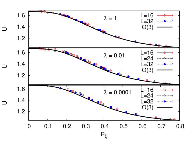
Figure 1: Estimates of $U$ versus $R_{\xi}$ for the $N=2$ model (with monopoles) for three different values of $\lambda$: $\lambda=1$ (top panel), $\lambda=10^{-2}$ (middle panel), $\lambda=10^{-4}$ (bottom panel). The continuous line is the universal curve for vector correlations in the O(3) vector model. Data approach the O(3) curve as the size increases.

‘

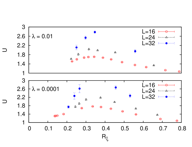
Figure 2: Estimates of $U$ versus $R_{\xi}$ for the $N=3$ model (with monopoles) for two different values of $\lambda$: $\lambda=10^{-2}$ (top panel), $\lambda=10^{-4}$ (bottom panel).

We have first studied the general model with Hamiltonian (1), without suppressing the monopole configurations. We consider systems with $N=2,3,4$, performing simulations for several values of the parameter $\lambda$.

For $N=2$ the transition always belongs to the O(3) universality class, with size corrections that are consistent with an $1/L^{\omega}$, $\omega\approx 0.8$, behavior (as expected in the O(3) case [28]), and that increase at fixed $L$ as $\lambda$ decreases. This is supported by the data shown in Fig. 1, where we plot the Binder parameter $U$ versus $R_{\xi}$ for three different values of $\lambda$, and compare the results with the universal asymptotic curve computed in the O(3) vector model. We observe a good agreement, confirming that the universal critical behavior is independent of the potential term in the Hamiltonian. To estimate the critical point, we have determined the values of $\beta$ for which $R_{\xi}(\beta)=R^{*}_{\xi}$ and $U(\beta)=U^{*}$, where $R^{*}_{\xi}$ and $U^{*}$ are the universal values that the two quantities take at the critical point in the O(3) universality class. Using the estimates [29] $R^{*}_{\xi}=0.564005(30)$ and $U^{*}=1.13933(4)$, we obtain $\beta_{c}=0.3082(3)$, 0.03958(2), 0.012766(1), and 0.004057(4) for $\lambda=1,10^{-2},10^{-3}$, and $10^{-4}$, respectively. Note that $\beta_{c}$ apparently scales as $\sqrt{\lambda}$ for $\lambda\to 0$, a behavior that can be understood as follows. In the mean-field approximation the minimum of the effective potential corresponds to $|w|^{2}=1+3\beta/(2\lambda)$, which indicates that $\langle|w|^{2}\rangle$ should increase as $\lambda\to 0$ roughly as $1+3\beta/(2\lambda)\approx\beta/\lambda$, a behavior that is supported by the numerical data. If we now rescale ${\bm{w}}=\langle|w|^{2}\rangle^{1/2}{\bm{z}}$, the nearest-neighbor interaction term becomes

$$-N\hat{\beta}\sum_{x,\mu}(\bar{\bm{z}}_{\bm{x}}\cdot{\bm{z}}_{{\bm{x}}+\hat{\mu}}\sigma_{{\bm{x}},\mu}+\hbox{c.c.})\qquad\hat{\beta}=\beta\langle|w|^{2}\rangle$$ (23)

We expect $\hat{\beta}_{c}\sim\beta_{c}^{2}/\lambda$ to be finite for $\lambda\to 0$, implying the expected behavior of $\beta_{c}$.

We have also studied the behavior for $N=3$ and 4. In both cases, we observe a first-order transition also for finite values of $\lambda$. In Fig. 2, we plot the Binder parameter $U$ for $N=3$ and $\lambda=10^{-2}$ and $10^{-4}$. It has a maximum that increases quite rapidly with the size of the system, as expected for a first-order transition. We have also analyzed the distributions of the order parameter $\mu_{2}$, observing two distinct peaks. Note that the identification of the transition as a first-order one becomes easier as $\lambda$ decreases. The CP² $(\lambda=\infty)$ model shows a very weak first-order transition, and a bimodal distribution for $\mu_{2}$ is only observed [25] for $L=96$. Instead, for $\lambda=10^{-2}$ and $10^{-4}$, the distribution is clearly bimodal already for $L=32$. For $N=4$ and small values of $\lambda$, the first-order transition is very strong already for $L=16$: We observe large hysteresis effects and we are not able to obtain equilibrated results.

4.2 Phase behavior of the monopole-free model with $N=2$

Figure 3: Plot of the specific heat $C$ as a function of $\beta$ in the transition region. Results for several values of $L$ up to $L=80$ for the $N=2$ MF model with $\lambda=0.01$. The curves interpolating the data with $L=48$, 60, and 80 are obtained using the multihistogram reweighting method [30].

Let us consider the MF model for $N=2$. For $\lambda=\infty$, Ref. [12] was not able to draw any definite conclusion on the order of the transition, in spite of extensive simulations on lattices of size up to $L=80$. Here we study the more general model, considering a very small value of $\lambda$, $\lambda=0.01$. This choice is motivated by the results of Section 4.1. If the transition for $\lambda=\infty$ is continuous, we expect the simulations for $\lambda=\infty$ and $\lambda=0.01$ to provide consistent results. This universality check would support the existence of a MF universality class for $N=2$. On the other hand, if no such universality class exists and the transition is of first order, one might hope the first-order nature of the transition to become more evident as $\lambda$ decreases, as it occurs in the presence of monopoles.

In Fig. 3 we report the specific heat $C$ as a function of $\beta$. It has a maximum for $\beta\approx 0.0325$ which increases with the size of the lattice. For each value of $L$ we have determined $C_{\rm max}(L)$. We have fitted the results to $aL^{\delta}$ including only data with $L\geq L_{\rm min}$, obtaining $\delta=0.58(1)$, 0.64(1), 0.68(1), 0.81(5) for $L_{\rm min}=16,20,28,48$. If we perform a fit to $aL^{\delta}+b$, i.e., if we include an analytic correction, we obtain $\delta=0.86(4),0.88(6),1.01(10)$ for $L_{\rm min}=16,20,28$. The results are analogous to those obtained for $\lambda=\infty$. Ref. [12] obtained $\delta=0.8(1)$ from the analysis of the specific heat using only data satisfying $L\geq 48$. The exponent $\delta$ is very different from the one expected for a first-order transition, $\delta=3$. If the transition is continuous, assuming the hyperscaling relation $2-\alpha=3\nu$, we can estimate $\nu$ using $\nu=2/(3+\delta)$. If $\delta=1.0(2)$, we would obtain $\nu=0.50(2)$, which is compatible with the estimate [12] $\nu=0.52(2)$ for the MFCP¹ model.

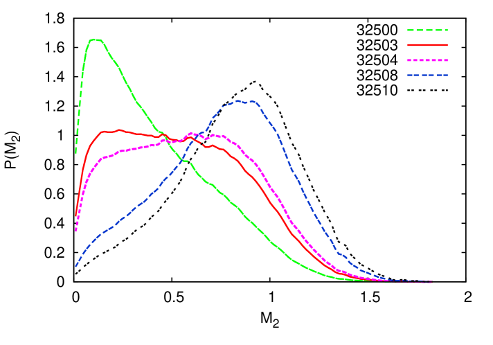
Figure 4: Distribution $P(M_{2})$ for the $N=2$ MF model with $\lambda=0.01$ for $L=60$ (top) and $L=80$ (bottom) for different values of $\beta$. The distributions are obtained using the multihistogram reweighting method [30]. In the legend we report $10^{6}\beta$; e.g., 32494 corresponds to $\beta=0.032494$.

Figure 5: Plot of the Binder parameter $U$ versus $R_{\xi}$, for several values of $L$ up to $L=80$ for the $N=2$ MF model with $\lambda=0.01$. The curves interpolating the data with $L=48$, 64, and 80 ($L$ increases moving rightward) are obtained using the multihistogram reweighting method [30]. In the inset we report the same interpolating curves (three rightmost curves) together with the analogous interpolating curves (three leftmost curves, again $L$ increases moving rightward) obtained for $\lambda=\infty$ (MFCP¹ model).

To better understand the nature of the transition, we have determined the distribution of $\mu_{2}$ defined in Eq. (17),

$$P(M_{2})=\langle\delta(M_{2}-\mu_{2})\rangle.$$ (24)

It is reported in Fig. 4 for several values of $\beta$. Although no double-peak structure is observed, the distribution varies as expected for a first-order transition, with a sharp change of the position of the peak as $\beta$ is varied. Finally, in Fig. 5 we report $U$ versus $R_{\xi}$. As already observed for $\lambda=\infty$, data do not scale. At fixed $R_{\xi}$, the estimates of $U$ are systematically increasing with $L$ for $0.2\leq R_{\xi}\lesssim 0.6$. However, we do not observe any systematic increase of the maximum of $U$ with $L$, as expected for a first-order transition. Precisely, using the multihistogram reweighting method [30], we estimate $U_{\rm max}(L)=1.77(1)$, 1.76(2), and 1.78(2) for $L=48,60$, and 80. It is interesting to compare the behavior of $U$ for $\lambda=\infty$ (MFCP¹ model; results from Ref. [12]) and $\lambda=0.01$ (see the inset of Fig. 5). The curves for the two different values of $\lambda$ are apparently unrelated. There is really no indication for universality, making the continuous-transition scenario rather unlikely.

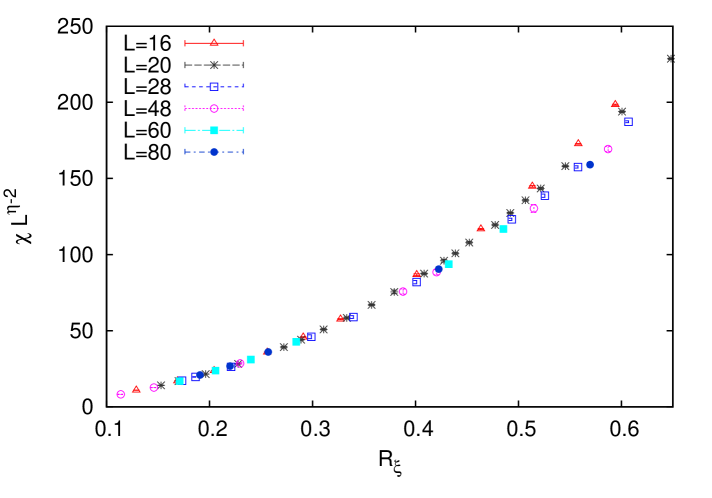
Figure 6: Plot of $\chi L^{\eta-2}$ as a function of $R_{\xi}$ with $\eta=0.223$. Results for the $N=2$ MF model with $\lambda=0.01$.

To conclude the analysis of the available data, we may assume that the transition is continuous and determine the critical exponents. We have first performed fits of $R_{\xi}$ and $U$ without including scaling corrections. The exponent $\nu$ and the transition value $\beta_{c}$ are determined by fitting the data to Eq. (21). The function $f_{R}(x)$ is approximated by a polynomial. The fits of $R_{\xi}$ have a large $\chi^{2}$, unless only data with $L\geq 48$ are included. In this case we obtain $\beta_{c}=0.0325086(9)$ and $\nu=0.54(2)$. If we use the same set of data for the Binder parameter, we obtain $0.0325114(7)$ and $\nu=0.43(1)$. The estimates of $\beta_{c}$ and of the exponent obtained from the two quantities are clearly not consistent. To understand whether these discrepancies are due to scaling corrections, we have performed combined fits of $R_{\xi}$ and $U$ to

$$R(\beta,L)=f_{R}(X)+L^{-\omega}g_{R}(X),$$ (25)

parametrizing $f_{R}(X)$ and $g_{R}(X)$ with polynomials. As before $X=(\beta-\beta_{c})L^{1/\nu}$. Fitting all data with $L\geq 16$, we obtain $\omega=0.1(1)$, $\nu=0.50(1)$, $\beta_{c}=0.32513(1)$. If we only include data with $L\geq 20$, we obtain consistent estimates for all quantities and $\chi^{2}/\hbox{DOF}\approx 1$ (DOF is the number of degrees of freedom of the fit). While the estimates of the exponents and of $\beta_{c}$ are reasonable, the estimates of the asymptotic curves $f_{R}(X)$ have large errors and, in some cases, they violate rigorous inequalities. For instance, the scaling curve $f_{U}(X)$ for the Binder parameter $U$ should always satisfy $f_{U}(X)>1$. This bound is violated for $X\gtrsim 0$. For instance, the fit predicts $f_{U}(0)=0.6(2)$. Therefore, the results of these fits cannot be trusted. This is not unexpected. If $\omega$ is so small, next-to-leading scaling corrections with exponents $2\omega$, $3\omega$, $\ldots$, should be included as well, to obtain meaningful results.

For $\lambda=\infty$ the best evidence [12] for a continuous transition was provided by the scaling behavior of the susceptibility $\chi$ defined in Eq. (14). This quantity scales as

$$\chi(\beta,L)\sim L^{2-\eta}\left[f_{\chi}(X)+O(L^{-\omega})\right],$$ (26)

or, equivalently, as

$$\chi(\beta,L)\sim L^{2-\eta}\left[F_{\chi}(R_{\xi})+O(L^{-\omega})\right].$$ (27)

For $\lambda=\infty$, data follow the scaling behavior (27) quite precisely with $\eta=0.335(10)$. We have repeated the same analysis using the present results for $\lambda=0.01$. We fit $\chi$ to $\ln\chi=(2-\eta)\log L+\hat{f}_{\chi}(R_{\xi})$, where we approximate the function $\hat{f}_{\chi}(x)$ with a polynomial in $x$. To estimate the role of the scaling corrections we include in the fit only the data corresponding to sizes $L\geq L_{\rm min}$. We obtain $\eta=0.239(6)$ and 0.208(17) for $L_{\rm min}=20$ and 28, respectively. In this case, scaling corrections appear to be small ($\chi^{2}$/DOF is approximately 1.4 for $L_{\rm min}=20$ and 0.1 for $L_{\rm min}=28$, if only data satisfying $R_{\xi}\leq 0.45$ are considered; DOF is the number of degrees of freedom of the fit), as is also evident from the scaling plot, Fig. 6 (in the figure we use $\eta=0.223$, which is the average of the results obtained for the two values of $L_{\rm min}$). Although results are consistent with the behavior expected at a continuous transition, note that universality is strongly violated: The estimate of $\eta$ differs from the one obtained in the MFCP¹ model [12], $\eta=0.335(10)$. It is closer to, though not in agreement with, the estimate [5] $\eta=0.259(6)$, obtained in a loop model that is expected [21, 22] to belong to the same universality class.

In conclusion, our results are apparently not consistent with a scenario in which the MF model with $N=2$ undergoes a continuous transition, unless scaling corrections decay with a very small exponent or logarithmically, as suggested in Ref. [31]. In our view, the most likely possibility is that the transition is of first order, but so weak that a clear signature can only be obtained on significantly larger lattices.

4.3 Results for $N=25$

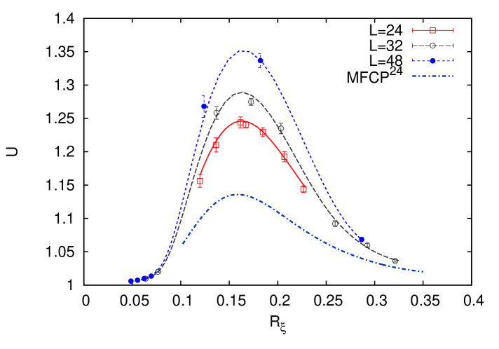
Figure 7: Plot of the Binder parameter $U$ versus $R_{\xi}$, for several values of $L$ for the MF model with $N=25$ and $\lambda=100$. The curves interpolating the data are obtained using the multihistogram reweighting method [30]. We also report an extrapolation (lower dot-dash line) of the data for the $\lambda=\infty$ model (MFCP²⁴ model).

Figure 8: Plot of the Binder parameter $U$ versus $R_{\xi}$, for several values of $L$ for $N=25$ for the model with partition function (28) and $a=\alpha=0.96$. The curves interpolating the data are obtained using the multihistogram reweighting method [30]. We also report an extrapolation (lower dot-dash line) of the data for the $\lambda=\infty$ model (MFCP²⁴ model).

We finally present our results for $N=25$. We have performed simulations on lattices of size $16\leq L\leq 48$ for several values of $\lambda$. For $\lambda=0.01$, 1, and 10, we observe a very strong first-order transition. If we first increase $\beta$ and then decrease it across the transition, a strong hysteresis is observed, even for $L$ as small as 12. For $\lambda=100$, data are again consistent with a first-order transition. In Fig. 7, we plot $U$ versus $R_{\xi}$. Data do not scale and the maximum $U_{\rm max}(L)$ increases with $L$, which is the typical signature of a first-order transition. In the same figure we also report an extrapolation of the data [12] obtained for the MFCP²⁴ model which is obtained in the limit $\lambda=\infty$. Also in the MFCP²⁴ model $U$ has a maximum, which is however significantly smaller than the maxima observed for $\lambda=100$. Clearly, the deviations observed for $\lambda=100$ cannot be interpreted as corrections to scaling.

To further explore the role that the size fluctuations of the field play, we have studied a different model that is easier to simulate and in which field-size fluctuations can be easily controlled. In the modified model the partition function is given by

$$Z=\int\prod_{{\bm{x}}\mu}d\sigma_{{\bm{x}}\mu}\prod_{{\bm{x}}}[d{\bm{w}}_{{\bm{x}}}d\bar{\bm{w}}_{{\bm{x}}}M({\bm{w}}_{\bm{x}})]\,e^{-\beta H_{\rm kin}}$$ (28)

where $H_{\rm kin}$ is defined in Eq. (2) and

$$M({\bm{w}})=|w|^{1-2N}[\delta(|{w}|-1)+\alpha\delta(|{w}|-a)].$$ (29)

In this model $|{w}|$ takes only two values, 1 and $a$. Field-size fluctations can be controlled by changing the parameters $a$ and $\alpha$. At $\beta=0$, the probabilities $P(|w|)$ of the two values are given by $P(1)=\cal N$ and $P(a)=\alpha{\cal N}$ with ${\cal N}=1+\alpha$. If $\beta$ is turned on, the probability $P(a)$ decreases with increasing $\beta$, since the kinetic term favors configurations with $|w|=1$. We performed simulations for $a=\alpha=0.96$, observing a transition for $\beta\approx 0.324$. In the critical region, we find $\langle w^{2}\rangle\approx 0.985$, so that $P(1)\approx 0.80$ and $P(a)\approx 0.20$. To compare the results obtained for this model with those obtained at fixed $\lambda$, we can compare the width of the fluctuations, defining

$$\sigma^{2}_{w^{2}}={\langle(|{w}|^{2}-\langle|{w}|^{2}\rangle)^{2}\rangle\over\langle|{w}|^{2}\rangle^{2}}.$$ (30)

In the model at fixed $\lambda=100$, we obtain $\sigma_{w^{2}}\approx 0.057$ in the whole critical region for $L=48$. In the new model, for the same value of $L$ we obtain $\sigma_{w^{2}}\approx 0.031$. Thus, in these simulations the fluctuations of $|{\bm{w}}|^{2}$ are reduced by a factor of 2.

Figure 9: Plot of the Binder parameter $U$ versus $R_{\xi}$, for several values of $L$ for $N=25$ for the model with partition function (28). We report: data obtained for the model with $a=0.9$ and $\alpha=2$ ($L=16,24$) and the interpolation (long dash; upper curve) of the $L=24$ data using the multihistogram reweighting method [30]; the interpolation (short dash; middle curve) of the data with $L=48$ for the model with $a=\alpha=0.96$; the extrapolation (dot dash; lower curve) of the data for the $\lambda=\infty$ model (MFCP²⁴ model).

The results for $a=0.96$ are consistent with a continuous transition, since we observe good scaling when we plot $U$ versus $R_{\xi}$, see Fig. 8. The results for different values of $L$, obtained using the multihystogram method [30], essentially fall on top of each other. However, note that the data scale onto a curve that is different from the one observed in the model at $\lambda=\infty$. For instance, in the present model $U_{\rm max}(L)=1.164(5)$, 1.163(5) for $L=32,48$, respectively. On the other hand, for the fixed-length model with $\lambda=\infty$, $U_{\rm max}(L)\approx 1.136$, see Fig. 8. Given the stability of the results, such large difference does not appear to be the result of scaling corrections, unless the subleading exponent is very small.

We have determined the exponent $\nu$ as before, fitting $U$ and $R_{\xi}$ to Eq. (21) using a polynomial approximation for the scaling function $f_{R}(x)$. We obtain:

$$\beta_{c}=0.32471(2),\qquad\nu=0.59(2),\quad U$$ from ;

$$\beta_{c}=0.324675(15),\qquad\nu=0.57(1),\quad R_{\xi}$$ from .

The estimates of the exponent and of $\beta_{c}$ obtained from the analysis of these two quantities are in substantial agreement. Moreover, the estimates of $\nu$ are consistent with the estimate $\nu=0.595(15)$ obtained in Ref. [12].

Finally, we study the critical behavior of the susceptibility $\chi$, performing fits to the ansatz

$$\ln\chi=(2-\eta)\ln L+\hat{f}_{\chi}(R_{\xi}).$$ (32)

We obtain $\eta=0.945(15),0.93(2)$ for $L_{\rm min}=24,32$, respectively, with a very good collapse of the data. However, these estimates are not consistent with the result $\eta=0.87(1)$ obtained in Ref. [12]. Again, universality is not observed.

To conclude, we have studied the same model, setting $a=0.9$ and $\alpha=2$, to increase the size of the field-length fluctuations. In the critical region, for $L=24$, we obtain $\langle|w|^{2}\rangle\approx 0.978$, $\sigma_{w^{2}}\approx 0.047$, $P(1)\approx 0.88$, and $P(a)\approx 0.12$. The plot of $U$ versus $R_{\xi}$ is shown in Fig. 9, for two values of $L$. In this case, data do not scale. The maximum $U_{\rm max}(L)$ of the Binder parameter increases with $L$, which provides some indication that the transition is not continuous.

In conclusion, the results we have obtained are not consistent with universality and are better explained in terms of a discontinuous transition, that becomes weaker as field-length fluctuations decrease. If we trust the results of Ref. [12], i.e., if we assume that the transition in the MFCP²⁴ model is continuous, we conclude that field-length fluctuations are relevant perturbations of the $N=25$ MF universality class. This implies that this critical behavior cannot have a simple field-theory interpretation. Indeed, in the field-theory approach the strength of the quartic potential parameters is always irrelevant. Of course, it is equally possible that no MF universality class exists. In that case the transition in the MFCP²⁴ model would be discontinuous. However, the correlation length at the transition would be finite but so large ($\xi\gtrsim 80$) that an apparent scaling behavior would be observed in the simulations with $L\leq 80$ as if the transition were continuous.

5 Conclusions

This paper reports a study of the phase diagram and of the nature of the phase transitions of 3D lattice models characterized by a global SU($N$) symmetry and a local U(1) symmetry. They generalize the lattice nearest-neighbor CP^N-1 model with an explicit gauge field—the corresponding Hamiltonian is given in Eq. (2). At variance with the CP^N-1 model, the length of the fields is not fixed, but is controlled by adding an appropriate potential parametrized by a parameter $\lambda$: for $\lambda\to\infty$ we reobtain the CP^N-1 model. We study the role that monopoles play in this class of systems, restricting the configuration space to gauge-field configurations in which no monopoles (we use the definition of Ref. [13]) are present. We perform Monte Carlo simulations for $N=2$ and 25, with the purpose of comparing the results for the present model with those obtained in Ref. [12] for the MFCP^N-1 model. The analysis of the finite-size data allows us to identify a finite-temperature transition in all cases, related to the condensation of a local gauge-invariant bilinear order parameter $Q_{\bm{x}}$, defined in Eq. (11).

For $N=2$ we performed simulations on relatively large systems, up to $L=80$. As it occurred for $\lambda=\infty$, we are not able to draw a definite conclusion on the nature of the transition. Many features are typical of first-order transitions. For instance, the Binder parameter data do not scale when plotted versus $R_{\xi}=\xi/L$, and the distributions of the order parameter and of the energy are quite broad, although without the typical bimodal shape that signals the presence of coexisting phases. On the other hand, the maximum of the Binder parameter does not increase with $L$, as it would be expected at first-order transitions. Assuming the transition to be continuous, we also estimate some critical exponents. The exponent $\nu$ is estimated from the finite-size behavior of $R_{\xi}$ and $U$. The fits, however, provide inconsistent estimates. Fits of the susceptibility give $\eta=0.22(2)$. The quality of the fit is good and we observe a good collapse of the data when $\chi L^{2-\eta}$ is plotted versus $R_{\xi}$. However, the estimate of $\eta$ differs significantly from the MFCP¹ result [12] $\eta=0.335(10)$, in contrast with universality.

Taking all results into account, the simplest scenario that explains the observed behavior is that of a weak first-order transition. It is so weak that coexisting phases can only be observed on very large lattices with $L\gg 80$, because of the presence of a large effective scale induced by the no-monopole condition. Of course, we cannot exclude, as suggested in the literature on quantum antiferromagnets, that the transition is continuous with very slowly decaying—even logarithmic [31], associated with a dangerously irrelevant variable—scaling corrections.

Finally, we have studied the MF model with $N=25$. We have performed simulations for several values of the potential parameter $\lambda$. For $\lambda=0.01,1$ and 10 we observe a strong first-order transition and a bimodal order-parameter distribution is already observed for lattice sizes as small as $L=12$. For $\lambda=100$, we do not observe a two-peak structure in the distributions of the energy or of the order parameter $\mu_{2}$ defined in Eq. (17). However, the rapid increase of the maximum of the Binder parameter with $L$ clearly points towards a discontinuous transition. We have also studied a different model in which the field length can only take two different values. In both cases, we find that the results for the two generalized models are not consistent with those obtained in the MFCP²⁴ model. They are better explained by a first-order transition scenario. These results cast doubts on the existence of a MF universality class for $N=25$. In any case, note that, if such universality class really exists, it cannot have a simple field-theory interpretation, since field-length fluctuations are apparently relevant perturbations in the renormalization-group sense. We do not think additional numerical work can provide new insight on these issues. A more promising approach is probably the $1/N$ expansion, in which some answers can be obtained analytically for large values of $N$.

References

References

- [1] Senthil T, Balents L, Sachdev S, Vishwanath A and Fisher M P A 2004 Quantum Criticality beyond the Landau-Ginzburg-Wilson Paradigm Phys. Rev. B 70, 144407
- [2] Motrunich O I and Vishwanath A 2004 Emergent photons and transitions in the O(3) -model with hedgehog suppression Phys. Rev. B 10, 075104
- [3] Bojesen T A and Sudbø A 2013 Berry phases, current lattices, and suppression of phase transitions in a lattice gauge theory of quantum antiferromagnets Phys. Rev. B 88, 094412
- [4] Block M S, Melko R G and Kaul R K 2013 Fate of CPN-1 fixed point with monopoles Phys. Rev. Lett. 111, 137202
- [5] Nahum A, Chalker J T, Serna P, Ortuño M and Somoza A M 2017 Deconfined Quantum Criticality, Scaling Violations, and Classical Loop Models Phys. Rev. X 5, 041048
- [6] Wang C, Nahum A, Metliski M A, Xu C and Senthil T 2017 Deconfined Quantum Critical Points: Symmetries and Dualities Phys. Rev. X 7, 031051
- [7] Sachdev S 2019 Topological order, emergent gauge fields, and Fermi surface reconstruction Rep. Prog. Phys. 82, 014001
- [8] Pelissetto A and Vicari E 2019 Multicomponent compact Abelian-Higgs lattice models Phys. Rev. E 100, 042134
- [9] Bonati C, Pelissetto A and Vicari E 2020 Higher-charge three-dimensional compact lattice Abelian-Higgs models Phys. Rev. E 102, 062151
- [10] Bonati C, Pelissetto A and Vicari E 2022 Critical behaviors of lattice U(1) gauge models and three-dimensional Abelian-Higgs gauge field theory Phys. Rev. B 105, 085112
- [11] Bonati C, Pelissetto A and Vicari E 2021 Lattice Abelian-Higgs model with noncompact gauge fields Phys. Rev. B 103, 085104
- [12] Pelissetto A and Vicari E 2020 Three-dimensional monopole-free CPN-1 models Phys. Rev. E 101, 062136
- [13] De Grand T A and Toussaint D 1980 Topological excitations and Monte Carlo simulation of Abelian gauge theory Phys. Rev. D 22, 2478
- [14] Halperin B I, Lubensky T C and Ma S K 1974 First-Order Phase Transitions in Superconductors and Smectic-A Liquid Crystals Phys. Rev. Lett. 32, 292
- [15] Folk R and Holovatch Y 1996 On the critical fluctuations in superconductors J. Phys. A 29, 3409
- [16] Ihrig B, Zerf N, Marquard P, Herbut I F and Scherer M M 2019 Abelian Higgs model at four loops, fixed-point collision and deconfined criticality Phys. Rev. B 100, 134507
- [17] Pelissetto A and Vicari E 2020 Large- behavior of three-dimensional lattice CPN-1 models J. Stat. Mech.: Th. Expt. 033209
- [18] Di Vecchia P, Holtkamp A, Musto R, Nicodemi F and Pettorino R 1981 Lattice CPN-1 models and their large- behaviour Nucl. Phys. B 190, 719
- [19] Irkhin V Yu, Katanin A A and Katsnelson M I 1996 expansion for critical exponents of magnetic phase transitions in the CPN-1 model for Phys. Rev. B 54, 11953
- [20] Moshe M and Zinn-Justin J 2003 Quantum field theory in the large limit: A review Phys. Rep. 385, 69
- [21] Nahum A, Chalker J T, Serna P, Ortuño M and Somoza A M 2011 3D Loop Models and the CPN-1 Model Phys. Rev. Lett. 107, 110601
- [22] Nahum A, Chalker J T, Serna P, Ortuño M and Somoza A M 2013 Phase transitions in three-dimensional loop models and the CPN-1 model Phys. Rev. B 88, 134411
- [23] Rabinovici E and Samuel S 1981 The CPN-1 model: A strong coupling lattice approach Phys. Lett. 101B, 323
- [24] Berg B and Lüscher M 1981 Definition and statistical distributions of a topological number in the lattice O(3) -model Nucl. Phys. B 190, 412
- [25] Pelissetto A and Vicari E 2019 Three-dimensional ferromagnetic CPN-1 models Phys. Rev. E 100, 022122
- [26] Challa M S S, Landau D P and Binder K 1986 Finite-size effects at temperature-driven first-order transitions Phys. Rev. B 34, 1841
- [27] Vollmayr K, Reger J D, Scheucher M and Binder K 1993 Finite size effects at thermally-driven first order phase transitions: A phenomenological theory of the order parameter distribution Z. Phys. B 91, 113
- [28] Pelissetto A and Vicari E 2002 Critical Phenomena and Renormalization Group Theory Phys. Rep. 368, 549
- [29] Hasenbusch M 2020 Monte Carlo study of a generalized icosahedral model on the simple cubic lattice Phys. Rev. B 102, 024406
- [30] Ferrenberg A M and Swendsen R H 1989 Optimized Monte Carlo data analysis Phys. Rev. Lett. 63, 1195
- [31] Sandvik A W 2010 Continuous Quantum Phase Transition between an Antiferromagnet and a Valence-Bond Solid in Two Dimensions: Evidence for Logarithmic Corrections to Scaling Phys. Rev. Lett. 104, 177201 Shao H, Guo W and Sandvik A W 2016 Quantum criticality with two length scales Science 352, 213