Abstract

Recent results from the intensity frontier indicate the tantalizing possibility of violation in lepton flavour universality. In light of this we revisit the minimal phenomenological $Z^{\prime}$ model taking in account both vectorial and axial-vectorial flavour violating couplings to the charged leptons. We make a systematic study to identify the minimal framework that can simultaneously explain the recent results on anomalous magnetic moment of muon and electron while remaining in consonance with $R_{K^{(*)}}$, $B^{0}_{s}-\bar{B^{0}_{s}}$ mixing and angular observables in the $B^{+}\to K^{+*}\mu^{+}\mu^{-}$ channel reported by the LHCb collaboration. We demonstrate that the neutrino trident data imply a further ${\rm SU(2)}_{L}$ violation in the leptonic couplings of the exotic $Z^{\prime}$.

1 Introduction

With continued improvement in resolution, the consistency of anomalous results from the intensity frontier may be the most significant indication of Beyond Standard Model (BSM) physics that we have today in hard experimental data.

Recently the measurement of the $(g-2)_{\mu}$ at the Fermi National Accelerator Laboratory (FNAL) [1] has added to this intrigue. The dramatic improvement in the resolution in the recent results has pushed the deviation from Standard Model (SM) prediction at $4.2~{}\sigma$ with $\Delta a_{\mu}=a_{\mu}^{\rm exp}-a_{\mu}^{\rm SM}\sim(251\pm 59)\times 10^{-11}.$ Notwithstanding the recent lattice results [2] this deviation has withstood scrutiny for some time now. Interestingly if one compares this with the status of $(g-2)_{e}$ measurement based on the Lawrence Berkeley National Laboratory (LBNL) determination of the structure constant based on cesium [3] one obtains a moderate deviation from SM at $2.4~{}\sigma,$ with the opposite pull at $\Delta a_{e}\sim(-8.8\pm 3.6)\times 10^{-13}$ [4]. This sign flip if true cannot be explained by simple mass scaling $\Delta a_{e}/\Delta a_{\mu}\sim m_{e}^{2}/m_{\mu}^{2}$ and should be construed as an indication of Lepton Flavour Universality Violation (LFUV) of any underlying New Physics (NP).

One can trace the imprint of this violation of lepton flavour universality in the rare decays of the $B$-mesons giving a more compelling experimental basis for the LFUV hypothesis. Indications of such LFUV can be seen in the flavour changing neutral current (FCNC) induced decays involving the $b\to sl^{+}l^{-}$ transitions. These are indeed easy picking ground in flavour physics searches for NP owing to the Glashow Iliopoulos Maiani (GIM) suppression of tree-level contribution to them within SM. In this context the observable $R_{K^{(*)}}$ is of significance as they are relatively independent of the form factor uncertainties [5, 6]. SM predictions [7, 8, 9] of these parameters exhibit $2-3~{}\sigma$ deviations from the corresponding experimental results reported by LHCb [10, 11]. Tying nicely with the paradigm of LFUV in underlying physics. Thus it is not surprising that there exists extensive literature that study various motivated BSM framework that tries to explain these anomalous results individually or in combinations [12, 13, 14, 15, 16, 17, 18, 19, 20, 21, 22, 23, 24, 25, 26, 27, 28, 29, 30, 31, 32, 33, 34, 35, 36, 37, 38, 39, 40, 41, 42, 43, 44, 45, 46, 47, 48, 49, 50, 51, 52, 53, 54, 55, 56, 57, 58, 59, 60, 61, 62, 63, 64, 65, 66, 67, 68, 69, 70, 71, 72, 73, 74, 75, 76, 77]. Moreover, after the declaration of the updated results [10, 1], several authors and collaboration published various articles in different existing and/or new BSM scenarios. Among the different categories of BSM frameworks, a kind of scenario with a non-standard neutral massive boson ($Z^{\prime}$) is very popular and effective, for the combined explanation of $R_{K}$ (including other $b\to sll$ anomalies) and $(g-2)_{\mu}$ [78, 79, 80, 81, 82, 83, 84, 85, 86, 87].

In the present paper we revisit one of the simplest of these framework that extends the SM to include an additional massive abelian gauge boson $Z^{\prime}$ with flavour violating couplings. With Occum’s razor in hand we build bottom up model of the $Z^{\prime}$ guided solely by the requirement of the experimental data remaining agnostic to any UV completion. Our approach is to pare down to the minimal version of the model that would be simultaneously in consonance with the various experimental results at low energy intensity frontiers with focus on observables that indicate LFUV. Our notion of simplicity will be guided by economy of new parameters rather than any symmetry or embedding considerations. Starting with the simplest two parameter model of $Z^{\prime}$ mass and universal couplings, we systematically build this phenomenological model of $Z^{\prime}$ from bottom up by adding new parameters as the experimental data demand the same. In this context, we demonstrate that the simultaneous inclusion of flavour violating vectorial and axial-vectorial couplings to the leptons is a prudent choice in constructing such minimal models.

Once we establish a data driven minimal phenomenological $Z^{\prime}$ model for LFUV we explore the region of parameter space of such a setup that would be in agreement with relevant experimental results including $B^{0}_{s}-\bar{B}^{0}_{s}$ mixing [88], recent LHCb results of angular observables in the $B^{+}\to K^{+*}\mu^{+}\mu^{-}$ channel [89] and some other constraints that are related to $b\to s$ transitions [90, 91, 92, 93]. We have also taken into account the constraints from collider and fixed target experiments [88, 94].

The article is organised as follows. In the Sec. 2 we explore different effective $Z^{\prime}$ scenarios in the context of recent data of $(g-2)_{\mu}$ and $(g-2)_{e}$. Then in Sec. 3 we resolve different anomalies related to $b\to sll$ transitions in a particular economic effective $Z^{\prime}$ scenario. After that in Sec. 4 we discuss the new results of LHCb related to angular observables of the decay $B^{+}\to K^{+*}\mu^{+}\mu^{-}$. We discuss our numerical results in Sec. 5. Then in Sec. 6 we comment on some relevant constraints. In Sec. 7 we re-examine the scenarios that we consider in this article in the context of latest experimental value of $(g-2)_{e}$ for which the $\Delta a_{e}$ is positive. Finally, in Sec. 8 we will conclude our findings.

2 Resolution of anomalous magnetic moment of charged lepton in minimal $Z^{\prime}$ scenario(s)

The magnetic moment $\vec{\mathbb{M}}$ of a charged lepton ($l$) can easily be defined in terms of its spin $\vec{\mathbb{S}}$ and gyromagnetic ratio ($g_{l}$) using the Dirac equation as follows

$$\vec{\mathbb{M}}=g_{l}\dfrac{e}{2\,m_{l}}\vec{\mathbb{S}}\,.$$ (1)

Ideally the value of $g_{l}$ is equal to 2. Quantum correction provides marginal shift within the SM. In order to estimate this deviation of $g_{l}$ from its tree-level value one can usually define the parameter,

$$a_{l}=\dfrac{g_{l}-2}{2}\,.$$ (2)

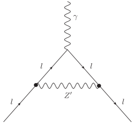
Figure 1: Relevant Feynman diagram that is contributed to the $(g-2)_{l}$ in addition to the SM.

We consider the extension of the SM incorporating a massive $Z^{\prime}$ as mass $M_{Z^{\prime}}$ having flavoured vectorial and axial-vectorial couplings as given by a generic effective Lagrangian,

$$\mathcal{L}\in\bar{l}\gamma^{\alpha}(a^{l}_{Z^{\prime}}+\gamma^{5}b^{l}_{Z^{\prime}})l~{}Z^{\prime}_{\alpha}\,,$$ (3)

where, $a^{l}_{Z^{\prime}}$ and $b^{l}_{Z^{\prime}}$ (where $l\in e,\mu$) are the vectorial and axial-vectorial couplings of light charged leptons with $Z^{\prime}$ boson. This leads to an additional contribution to the anomalous magnetic moment of charged lepton depicted in Fig. 1 and the corresponding contribution is given by [95, 67, 39, 43],

$$\Delta a_{l}^{Z^{\prime}}=\frac{1}{8\pi^{2}}~{}\left((a^{l}_{Z^{\prime}})^{2}F_{a^{l}_{Z^{\prime}}}(R_{Z^{\prime}})-(b^{l}_{Z^{\prime}})^{2}F_{b^{l}_{Z^{\prime}}}(R_{Z^{\prime}}))\right)\,,\\$$ (4)

with $R_{Z^{\prime}}\equiv M^{2}_{Z^{\prime}}/m^{2}_{l}$. Here, $M_{Z^{\prime}}$ is the mass of $Z^{\prime}$ boson and $m_{l}$ is the mass of charged lepton. The loop functions corresponding to vectorial and axial-vectorial interactions are given as follows,

$$F_{a^{l}_{Z^{\prime}}}(R_{Z^{\prime}}) = \int_{0}^{1}dx\,\frac{2x(1-x)^{2}}{(1-x)^{2}+R_{Z^{\prime}}x}\;,$$ (5)

$$F_{b^{l}_{Z^{\prime}}}(R_{Z^{\prime}}) = \int_{0}^{1}dx\,\frac{2x(1-x)(3+x)}{(1-x)^{2}+R_{Z^{\prime}}x}\;.$$ (6)

2.1 The Minimal Model

We now embark on identifying the minimal flavoured model of $Z^{\prime}$ that can explain the anomalous magnetic moment of the charged leptons. Our hunt will be guided by the recent experimental data on the anomalous magnetic moment of the charged leptons that we now briefly summarise:

• In the case of muon ($\mu$), over the last two decades there is an enduring deviation ($\gtrapprox 3.5\sigma$) between theoretical prediction and the corresponding experimental data. Recently, a measurement of the $(g-2)_{\mu}$ has been reported by FNAL [1],

  $$a_{\mu}^{\rm exp}=116592061\pm 41\times 10^{-11}\,.$$ (7)

  The state of the art SM theoretical prediction is [96]

  $$a_{\mu}^{\rm SM}=116591810\pm 43\times 10^{-11}\,.$$ (8)

  This amounts to a disagreement between SM prediction and experiment at $4.2\sigma$ parametrised by,

  $$\Delta a_{\mu}=a_{\mu}^{\rm exp}-a_{\mu}^{\rm SM}=(251\pm 59)\times 10^{-11}\,.$$ (9)

• Similarly there exists a milder disagreement if we compare theoretical and experimental values of $(g-2)$ in the electronic sector. For example, SM prediction of $(g-2)_{e}$ [97] was determined with the value of fine structure constant, evaluated at the Berkeley laboratory by performing high precision measurement using cesium atoms [3]. This value moderately deviates ($\simeq 2.4\sigma$) from the corresponding experimental result [4] and is parametrised as,

  $$\Delta a_{e}=a_{e}^{\rm exp}-a_{e}^{\rm SM}=(-8.8\pm 3.6)\times 10^{-13}\,.$$ (10)

  Interestingly the deviation in the anomalous magnetic moment for the electronic and muonic sector have opposite sign. It is difficult to account for this from a simple mass scaling ($\Delta a_{e}/\Delta a_{\mu}\sim m^{2}_{e}/m^{2}_{\mu}\sim 10^{-5}$). This can be construed as an evidence of lepton flavour non-universality of any underlying NP. In this paper we systematically study the minimal flavoured $Z^{\prime}$ model that can simultaneously explain the deviation in the anomalous magnetic moment in the electronic and muonic sector.

1. First we consider that the $Z^{\prime}$ has universal vectorial interaction with charged lepton with the effective Lagrangian of the form,

   $$\mathcal{L}\in\bar{l}\gamma^{\alpha}(a_{Z^{\prime}})l~{}Z^{\prime}_{\alpha}\,,$$ (11)

   where, $l\in(e,\mu)$. This scenario has two free parameters $M_{Z^{\prime}}$ and $a_{Z^{\prime}}$. With this setup, while one can tune $a_{Z^{\prime}}$ to explain the result of anomalous magnetic moment of muon. However, there is no possibility to explain the relative sign difference between the two leptonic generation.

2. We now consider non-zero vectorial ($a_{Z^{\prime}}$) and axial-vectorial ($b_{Z^{\prime}}$) couplings with both muon and electron. The effective interaction is given by,

   $$\mathcal{L}\in\bar{l}\gamma^{\alpha}(a_{Z^{\prime}}+\gamma^{5}b_{Z^{\prime}})l~{}Z^{\prime}_{\alpha}.$$ (12)

   This extends the number of free parameters to three viz $a_{Z^{\prime}}$, $b_{Z^{\prime}}$ and $M_{Z^{\prime}}$. This is still unable to simultaneously explain the measured value of $\Delta a_{\mu}$ and $\Delta a_{e}$. The region of the parameter space allowed by $\Delta a_{\mu}$ and $\Delta a_{e}$ individually are shown in Fig. 2a in $a_{Z^{\prime}}$ vs $b_{Z^{\prime}}$ plane for different values of $M_{Z^{\prime}}$ in the range [$10^{-3}$ to $10^{3}$] GeV. We obtain no overlap at al.

   

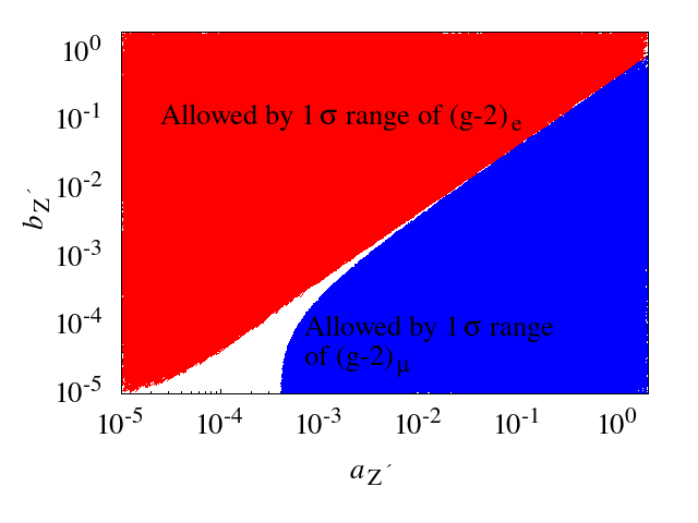
   (a)

   

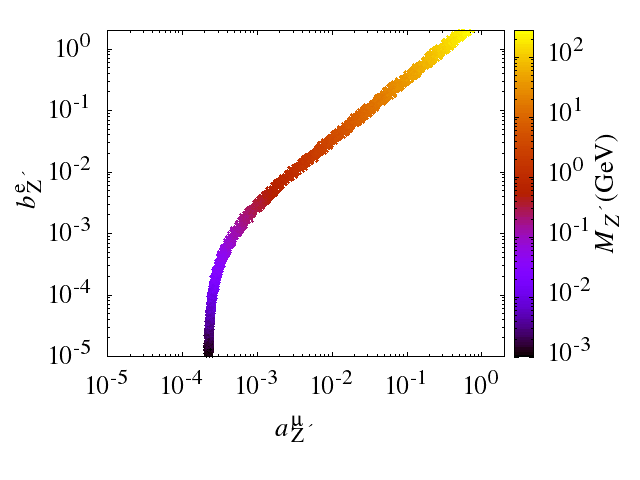
   (b)

   Figure 2: Left panel: 1$\sigma$ allowed parameter space by $(g-2)_{\mu}$ (blue) and $(g-2)_{e}$ (red) in $a_{Z^{\prime}}$ and $b_{Z^{\prime}}$ plane. Right panel: 1$\sigma$ allowed parameter space in $a^{\mu}_{Z^{\prime}}$ vs $b^{e}_{Z^{\prime}}$ plane with the allowed values of $M_{Z^{\prime}}$ (in GeV).

3. Keeping with three parameter models we now explore the possibility of addressing the anomalous magnetic moments using an interaction of the following form,

   $$\mathcal{L}\in\bar{\mu}\gamma^{\alpha}(a^{\mu}_{Z^{\prime}})\mu~{}Z^{\prime}_{\alpha}+\bar{e}\gamma^{\alpha}(\gamma^{5}b^{e}_{Z^{\prime}})e~{}Z^{\prime}_{\alpha}\,.$$ (13)

   With these combination one can simultaneously explain the $(g-2)_{\mu}$ and $(g-2)_{e}$ data at al. We have shown the allowed parameter space in $a^{\mu}_{Z^{\prime}}$ vs $b^{e}_{Z^{\prime}}$ plane while the values of $M_{Z^{\prime}}$ are shown by colour codes. Expectedly with increasing values of $a^{\mu}_{Z^{\prime}}$ and $b^{e}_{Z^{\prime}}$ a large $M_{Z^{\prime}}$ is required to reduce the loop effects by suppressing the propagator as can be read off from Fig. 2b.

3 LFUV From $B$-sector

A synergy of experimental results in the decay of $B$-meson provide further credence to the emergent paradigm of LFUV. As for example $R_{K^{(*)}}$ define as [99],

$$R_{K^{(*)}}\equiv\frac{\int^{q^{2}_{\rm max}}_{q^{2}_{\rm min}}\frac{d\Gamma\left({B}\rightarrow K^{(*)}\mu^{+}\mu^{-}\right)}{dq^{2}}dq^{2}}{\int^{q^{2}_{\rm max}}_{q^{2}_{\rm min}}\frac{d\Gamma\left({B}\rightarrow K^{(*)}e^{+}e^{-}\right)}{dq^{2}}dq^{2}}\;,$$ (14)

where $q^{2}$ represents the dilepton mass squared with the limits $q^{2}_{\rm max}=(m_{B}-m_{K^{(*)}})^{2}$, $q^{2}_{\rm min}=4m^{2}_{l}$ and $m_{B}$ represents the mass of $B$-meson. When QED corrections are included in the SM, these ratios are close to modulo one [100]. We summarise some of the relevant FCNC related experimental parameters in Table 1. The imprint of NP in this data is becoming increasingly apparent.

Observable	SM prediction		Measurement		Deviations
$R_{K}:q^{2}=[1.1,6]\,\text{GeV}^{2}$	$1.00\pm 0.01$	[7, 8]	$0.846^{+0.042+0.013}_{-0.039-0.012}$	[10]	3.1$\sigma$
$R_{K^{*}}^{\rm low}:q^{2}=[0.045,1.1]\,\text{GeV}^{2}$	$0.92\pm 0.02$	[9]	$0.660^{+0.110}_{-0.070}\pm 0.024$	[11]	$2.1\sigma-2.3\sigma$
$R_{K^{*}}^{\rm central}:q^{2}=[1.1,6]\,\text{GeV}^{2}$	$1.00\pm 0.01$	[7, 8]	$0.685^{+0.113}_{-0.069}\pm 0.047$	[11]	$2.4\sigma-2.5\sigma$

Table 1: The experimental values of $R_{K}$ and $R_{K^{*}}$ along with their SM predictions for different ranges of $q^{2}$.

Considering this, we now proceed to check the compatibility of the minimal $Z^{\prime}$ model discussed in the previous section with the experimental data related to $b\to sll$ transitions. With this non-universal nature of the coupling of $Z^{\prime}$ to $e$ and $\mu$ it is expected that the decay widths for $b\to s\mu^{+}\mu^{-}$ and $b\to se^{+}e^{-}$ will be different. The possibility to exploit this property to resolve the above mentioned LFUV anomalies is optimistic. In order to couple to the quark sector we introduce a single new flavour off diagonal interaction with coupling $\textsl{g}_{bs}$

$$\Delta\mathcal{L}\in\textsl{g}_{bs}(\bar{b}\gamma^{\alpha}P_{L}s)Z^{\prime}_{\alpha}\,,$$ (15)

in addition to the Lagrangian given in Eq. 13. In the rest of this paper, we refer to this minimally flavoured scenario as MFS. The effective interaction between $bsZ^{\prime}$ imply new contribution to the ${B^{0}_{s}}-\bar{B^{0}_{s}}$ oscillation at tree-level. This can provide stringent constraint in the parameter space and thus we incorporate the constraint of ${B^{0}_{s}}-\bar{B^{0}_{s}}$ oscillation in our analysis.

The analysis that follows our approach is to reconstruct the flavour observables using their proper definition within MFS and implement them in our numerical analysis. This may be contrasted with the approach where fit values of Wilson Coefficients (WCs) are utlised.

3.1 The $B\to K^{(*)}l^{+}l^{-}$ transition

The hadronic decay $B\to K^{(*)}l^{+}l^{-}$ is driven by the underlying transition $b\to sl^{+}\l^{-}$ at the quark level. The effective Hamiltonian at hadronic scale $Q\sim m_{b}$ is given by [101]

$$\centering{\cal H}_{\rm eff}(b\to sl^{+}l^{-})={\cal H}_{\rm eff}(b\to s\gamma)-\frac{G_{\rm F}}{\sqrt{2}}\frac{\alpha_{\rm em}}{\pi}V_{ts}^{*}V_{tb}\left[C_{9}(Q)\mathcal{O}_{9}+C_{10}(Q)\mathcal{O}_{10}\right]\,,\@add@centering$$ (16)

where,

$$\mathcal{O}_{9}=(\bar{s}\gamma^{\alpha}P_{L}b)(\bar{l}\gamma_{\alpha}l)\,,\qquad\mathcal{O}_{10}=(\bar{s}\gamma^{\alpha}P_{L}b)(\bar{l}\gamma_{\alpha}\gamma_{5}l)\,,$$ (17)

are the two crucial operators for this transition. In the first part of the Hamiltonian (see Eq. 16) there is no NP contribution, while in the remaining part, along with the SM contribution there is NP contribution from tree-level $Z^{\prime}$ exchange (see Fig. 3). Since $Z^{\prime}$ is assumed to couple only to left handed SM fermion, therefore the corresponding chirality flipped operators are not generated. The relevant WCs corresponding to the operators $\mathcal{O}_{9}$ and $\mathcal{O}_{10}$ have contained the tree-level NP contributions from a phenomenological $Z^{\prime}$ define in Eqs. 13 and 15 are given by [102],

$$C^{\rm NP}_{9} = -\frac{\sqrt{2}\pi}{G_{F}\alpha_{\text{em}}V_{ts}^{*}V_{tb}}\frac{\textsl{g}_{bs}a^{\mu}_{Z^{\prime}}}{M^{2}_{Z^{\prime}}}\,,$$ (18)

$$C^{\rm NP}_{10} = -\frac{\sqrt{2}\pi}{G_{F}\alpha_{\text{em}}V_{ts}^{*}V_{tb}}\frac{\textsl{g}_{bs}b^{e}_{Z^{\prime}}}{M^{2}_{Z^{\prime}}}\,,$$ (19)

where $G_{F}$ is the Fermi constant, $\alpha_{\text{em}}$ represents the fine structure constant and $V_{ij}$ stands for the Cabibbo Kobayashi Maskawa (CKM) matrix elements.

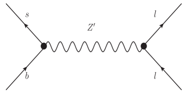
Figure 3: Tree-level Feynman diagram that contributes to $b\to sl^{+}l^{-}$ transition mediated by $Z^{\prime}$ boson.

3.1.1 $R_{K}$

In light of the recent result on the differential distribution of the $B^{+}\to K^{+}l^{+}l^{-}$ transitions from LHCb [10] in this section we briefly discuss the decay distribution of this transition. The differential branching fraction for $B^{+}\to K^{+}l^{+}l^{-}$ is written as [103]

$$\frac{d\Gamma(B^{+}\to K^{+}l^{+}l^{-})}{dq^{2}}=\frac{G_{F}^{2}\alpha^{2}_{\text{em}}|V_{tb}V_{ts}^{*}|^{2}}{2^{10}\pi^{5}m_{B}^{3}}\lambda^{3/2}(m_{B}^{2},m_{K}^{2},q^{2})\left(|F_{V}|^{2}+|F_{A}|^{2}\right),$$ (20)

where,

$$\lambda(a,b,c) =a^{2}+b^{2}+c^{2}-2(ab+bc+ac)\,,$$ (21)

$$F_{V}(q^{2}) =C_{9}^{\text{eff}}(q^{2})f_{+}(q^{2})+\frac{2m_{b}}{m_{B}+m_{K}}C_{7}^{\text{eff}}f_{T}(q^{2})\,,$$ (22)

$$F_{A}(q^{2}) =C_{10}f_{+}(q^{2})\,.$$ (23)

For completeness we have given the relevant expressions for the WCs in Appendix A. $f_{+}$ and $f_{T}$ are the relevant form factors. Corresponding details are given in the Appendix B.1. Using the Eqs. 20 and 14 we can evaluate the $R_{K}$.

3.1.2 $R_{K^{*}}$

Similar to the earlier section, in order to determine the $R_{K^{*}}$ here we would like to calculate the differential decay rate of $B\to K^{0*}l^{+}l^{-}$ with respect to $q^{2}$ and which is given as follows [104, 105]

$$\frac{d\Gamma(B^{0}\to K^{0*}l^{+}l^{-})}{dq^{2}} = \frac{1}{4}(3I_{1}^{c}+6I_{1}^{s}-I_{2}^{c}-2I_{2}^{s})\;.$$ (24)

Using the above expression and Eq. 14 we can determine the observable $R_{K^{*}}$. The angular coefficients $I^{c,s}_{1,2}$ that are involved in the above Eq. 24 can be defined as follows [106]

$$I_{1}^{s} = \frac{(2+\beta_{l}^{2})}{4}\left[|{A_{\perp}^{L}}|^{2}+|{A_{\parallel}^{L}}|^{2}+(L\to R)\right]+\frac{4m_{l}^{2}}{q^{2}}\text{Re}\left({A_{\perp}^{L}}{A_{\perp}^{R}}^{*}+{A_{\parallel}^{L}}{A_{\parallel}^{R}}^{*}\right),$$ (25)

$$I_{1}^{c} = |{A_{0}^{L}}|^{2}+|{A_{0}^{R}}|^{2}+\frac{4m_{l}^{2}}{q^{2}}\left[|A_{t}|^{2}+2\text{Re}({A_{0}^{L}}{A_{0}^{R}}^{*})\right],$$ (26)

$$I_{2}^{s} = \frac{\beta_{l}^{2}}{4}\left[|{A_{\perp}^{L}}|^{2}+|{A_{\parallel}^{L}}|^{2}+(L\to R)\right],$$ (27)

$$I_{2}^{c} = -\beta_{l}^{2}\left[|{A_{0}^{L}}|^{2}+(L\to R)\right],$$ (28)

with $\beta_{l}=\sqrt{1-4m_{l}^{2}/q^{2}}$. The functions $A_{L/R,i}$ are called the transversity amplitudes that can be decomposed in terms of appropriate WCs and form factors. Details of the relevant form factors are provided in Appendix B.2. The WCs ($C_{9}$ and $C_{10}$) are containing the NP contributions from $Z^{\prime}$ exchange (see Eqs. 18 and 19). The complete expressions for the transversity amplitudes have been given in Appendix C.

3.2 Constraint from ${B^{0}_{s}}-\bar{B^{0}_{s}}$ mixing due to tree-level contributions of $Z^{\prime}$

In this section we discuss the constraint from the mass difference ($\Delta M_{s}$) between the ${B^{0}_{s}}$ meson mass eigenstates arising from the ${B^{0}_{s}}-\bar{B^{0}_{s}}$ mixing phenomena. The SM contribution to this $\Delta B=2$ transition process through the top quark mediated box-diagram [107, 108] and is numerically given as [109] $(\Delta M_{s})_{\rm SM}=(18.77\pm 0.86){\rm ps}^{-1}$ that is in good agreement with experimental value [88] $(\Delta M_{s})_{\rm exp}=(17.749\pm 0.019\pm 0.007){\rm ps}^{-1}$.

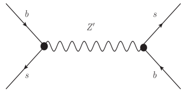
Figure 4: Tree-level Feynman diagram that contributes to ${B^{0}_{s}}-\bar{B^{0}_{s}}$ transition mediated by $Z^{\prime}$ boson.

In the minimal flavoured $Z^{\prime}$ model there exists a tree-level $Z^{\prime}$ contribution depicted in Fig. 4 and can be defined as [102]

$$\Delta M_{s}(Z^{\prime})=\left[\frac{g_{bs}}{V^{*}_{ts}V_{tb}}\right]^{2}\frac{4\tilde{r}\pi\sin^{2}\theta_{W}}{\sqrt{2}G_{F}\alpha_{\text{em}}M^{2}_{Z^{\prime}}},$$ (29)

with

$$\tilde{r}=\frac{C_{1}^{\rm VLL}(M_{Z^{\prime}})}{0.985}\eta_{6}^{6/21}\left[1+1.371\frac{\alpha_{s}^{(6)}(m_{t})}{4\pi}(1-\eta_{6})\right],$$ (30)

where,

$$C_{1}^{\text{VLL}}(Q)=1+\frac{\alpha_{s}}{4\pi}\left(-2\log\frac{M_{Z^{\prime}}^{2}}{Q^{2}}+\frac{11}{3}\right)\;.$$ (31)

The above quantity depicts ${\cal O}(\alpha_{s})$ QCD corrections to $Z^{\prime}$ tree-level exchange [110] and the two factors containing

$$\eta_{6}=\frac{\alpha_{s}^{(6)}(M_{Z^{\prime}})}{\alpha_{s}^{(6)}(m_{t})}\;,$$ (32)

designate together NLO QCD renormalisation group evolution from top quark mass ($m_{t}$) to $M_{Z^{\prime}}$ as given in [111]. In our scan we restrict the value of ${(\Delta M_{s})_{\rm exp}}/{(\Delta M_{s})_{\rm SM}}$ within the 2 $\sigma$ allowed range $(0.946\pm 0.086)$.

4 Angular observables for $B^{+}\to K^{+*}\mu^{+}\mu^{-}$ transition

The LHCb collaboration recently reported results for angular observables of the $B^{0}\to K^{0*}\mu^{+}\mu^{-}$ channel [112]. Interestingly, the observation by LHCb collaboration [112] on the $B^{0}\to K^{0*}\mu^{+}\mu^{-}$ decay channel is in tension with respect to the SM prediction of observable $P^{\prime}_{5}$. Similarly, a latest data of LHCb with 9${\rm fb}^{-1}$ luminosity [89] has provided the first measurement of the full set of CP-averaged angular observables in the isospin partner decay $B^{+}\to K^{+*}\mu^{+}\mu^{-}$. In this case the $K^{+*}$-meson reconstructed through the decay chain $K^{+*}\to K^{0}_{S}\pi^{+}$ with $K^{0}_{S}\to\pi^{+}\pi^{-}$. For a particular angular observable $P_{2}$ in the $6.0-8.0$ ${\rm GeV}^{2}$ interval there is the largest local disagreement with respect to the SM prediction. The corresponding deviation is around $3\sigma$. Considering this, using the definition given in [113] we evaluate CP-averaged angular observables $P_{2}$ and $P^{\prime}_{5}$. With these observables, we further impose the constraint in the parameter space of the MFS. We have considered the given CP-averaged binned data (for different $q^{2}$ values given in [89] ) for the angular observables. The expressions for the observables $P_{2}$ and $P^{\prime}_{5}$ containing NP contribution from the MFS can be written as,

$$P_{2} = \beta_{l}\frac{I^{s}_{6}}{8I_{2}^{s}}~{}~{}~{}{\rm with}~{}~{}~{}I_{6}^{s}=2\beta_{l}\left[\text{Re}({A_{\parallel}^{L}}{A_{\perp}^{L}}^{*})-(L\to R)\right]\;,$$ (33)

$$P_{5}^{\prime} = \frac{I_{5}}{2\sqrt{-I_{2}^{c}I_{2}^{s}}}~{}~{}~{}{\rm with}~{}~{}~{}I_{5}=\sqrt{2}\beta_{l}\left[\text{Re}({A_{0}^{L}}{A_{\perp}^{L}}^{*})-(L\to R)\right]\;,$$ (34)

where, $I^{s}_{2}$ and $I^{c}_{2}$ are given in Eqs. 27 and 28 respectively. With the given data and the corresponding theoretical predictions in MFS we have derived $\chi^{2}$ per degrees of freedom. Then using this we have imposed the condition on the parameter space which is allowed by 95% C.L. of the given data for $P_{2}$ and $P^{\prime}_{5}$. Here, we would like to mention that in our analysis we have not considered the bin [6.0, 8.0] GeV² of $q^{2}$ since it is known to suffer from long distance $c\bar{c}$ corrections close to the open charm threshold.

5 Numerical results

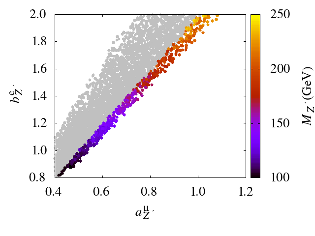
(a)

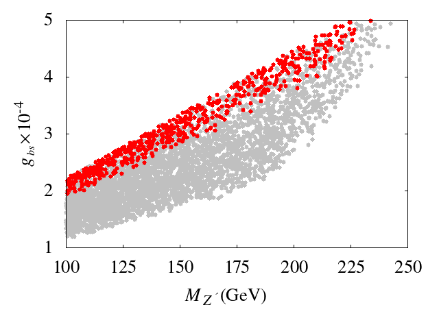
(b)

Figure 5: Left panel: Allowed parameter space in $a^{\mu}_{Z^{\prime}}$ vs $b^{e}_{Z^{\prime}}$ plane with allowed values of the mass $Z^{\prime}$ boson (in GeV). Different values of masses are indicated by different colour code. Right panel: Allowed parameter space in $M_{Z^{\prime}}$ (in GeV) vs $\textsl{g}_{bs}$ plane. For both the panel, we have taken the current experimental results of $(g-2)_{\mu}$, $(g-2)_{e}$ (with negative value of $\Delta a_{e}$), latest data of $R_{K}$, $R_{K^{*}}$, leading angular observables ($P_{2}$ and $P^{\prime}_{5}$) of $B^{+}\to K^{+*}\mu^{+}\mu^{-}$ decay mode. Further, we have taken the constraint that is imposed by the ${B^{0}_{s}}-\bar{B^{0}_{s}}$ mixing. If we relax the angular observables conditions then there will be an enhancement of the allowed parameter space and which is reflected by the grey coloured region in both the panels.

We have performed an extensive numerical scan sampling over $10^{7}$ points using the free parameters in MFS. From this scan, about four thousand ($0.04\%$) points survive which satisfy the latest measurement of $\Delta a_{\mu}$ at Fermilab [1], $\Delta a_{e}$ given by Barkeley laboratory [3], $R_{K}$ published by LHCb collaboration [10], up to date results of $R_{K^{*}}$ for the both lower and central bin values of $q^{2}$ [11]. Moreover, we incorporate relevant constraint from ${B^{0}_{s}}-\bar{B^{0}_{s}}$ oscillation data [88]. Additionally we have also imposed the constraints from the leading angular observables ($P_{2}$ and $P^{\prime}_{5}$) of $B^{+}\to K^{+*}\mu^{+}\mu^{-}$ decay mode [89]. In the left panel (5a) of Fig. 5 we have shown the allowed parameter space in $a^{\mu}_{Z^{\prime}}$ vs $b^{e}_{Z^{\prime}}$ plane with allowed values of the mass of $Z^{\prime}$ boson (indicated by different colour code). This pattern can be explained if we consider the similar argument as given for the Fig. 2b. However, in the case of Fig. 5 apart from the case of $(g-2)_{l}$, we have to consider the NP contributions to the WCs $C_{9}$ and $C_{10}$ for $B$-meson decays. If one looks at the Eqs. 18 and 19, then it is evident that the NP contributions to WCs $C_{9}$ and $C_{10}$ are proportional to ${a^{\mu}_{Z^{\prime}}}/{M^{2}_{Z^{\prime}}}$ and ${b^{e}_{Z^{\prime}}}/{M^{2}_{Z^{\prime}}}$ respectively. Therefore, if the values of $a^{\mu}_{Z^{\prime}}$ and $b^{e}_{Z^{\prime}}$ are increased then in order to restrict the numerical prediction of the observables within the allowed range, the values of $M_{Z^{\prime}}$ will also increase to suppress the propagator effect and it is depicted in the left panel (5a) of Fig 5. Similar argument also holds good for the right panel (5b) and it is evident from the Eqs. 18 and 19. Hence, following the previous argument and from the Eqs. 18 and 19 it is clear that with the increasing values of $\textsl{g}_{bs}$ the values of $M_{Z^{\prime}}$ will also increase and it is reflected from the right panel (5b) of the Fig. 5. If we relax the constraints from angular observables of the $B^{+}\to K^{+*}\mu^{+}\mu^{-}$ decay mode, we expectedly obtain an enlarged allowed parameter space and these additional points are depicted in grey in both the panels of Fig. 5.

5.1 Some relevant constraints regarding $b\to s$ decay transitions

Some comments on processes related $b\to s$ transitions are now in order. In our minimal scenario constraint from Br($B_{s}\to\mu^{+}\mu^{-}$) is not relevant, because it is dominated by the WC $C_{10}$. In this scenario, the WC $C_{9}$ gets the NP contribution for the $b\to s\mu^{+}\mu^{-}$ transition whereas the WC $C_{10}$ receives the NP contribution for $b\to se^{+}e^{-}$ transition due to the presence of non zero value of $b^{e}_{Z^{\prime}}$. Therefore, we have computed Br$(B_{s}\to e^{+}e^{-})$ for allowed parameter points shown in the Fig. 5. Consequently, we have found that due to NP contribution there is a substantial amount of enhancement to the Br$(B_{s}\to e^{+}e^{-})$ with respect to the corresponding SM prediction $8.6\times 10^{-14}$ [90]. This can be construed as an testable prediction of this framework. For example, if we consider the value of $M_{Z^{\prime}}$ is 180 GeV then within the allowed region of parameter space the model prediction for the Br$(B_{s}\to e^{+}e^{-})$ can be as large as $2.43\times 10^{-12}$ which is well below the experimental upper limit value $9.4\times 10^{-9}$ [90]. Moreover, we have found that within the allowed values of $M_{Z^{\prime}}$ (e.g., between 100 GeV to 200 GeV), the largest values of Br$(B_{s}\to e^{+}e^{-})$ almost remain the same. Further, we have checked that parameter space (presented in the Fig. 5) is also in consonance with the experimental results for the decays $B\to K^{(*)}e^{+}e^{-}$ [91, 92].

6 Other experimental constraints

We now turn our attention to other relevant bounds on the effective $Z^{\prime}$ scenario from searches at both low energy and high energy collider experiments.

In most UV complete models where an exotic $Z^{\prime}$ couples to the charged leptons, an interaction with the corresponding neutrinos is naturally expected. In fact in the limit of preserved ${\rm SU(2)}_{L}$ symmetry we expect identical coupling between the left handed charged leptons and their isospin partner neutrinos. Additional constraints that arise due to the coupling of the $Z^{\prime}$ to the neutrinos are summarised below:

1. The CCFR experiment has put stringent bounds on muon neutrino-nucleus scattering cross section ($\nu_{\mu}(\overline{\nu_{\mu}})+N\rightarrow\nu_{\mu}(\overline{\nu_{\mu}})+\mu^{+}\mu^{-}+N$) that can provide constraint on the parameter space of interest. The neutrino trident production cross section measured at the CCFR experiment at ${\sigma_{\rm CCFR}}/{\sigma_{\rm SM}}=0.82\pm 0.28$ [94].

2. Measurement of Br($B\to K^{(*)}\nu\bar{\nu}$) by the Belle collaboration [93] can also potentially constrain the $Z^{\prime}-\nu$ couplings.

It is known that the neutrino trident production cross section excludes the $(g-2)_{\mu}$ allowed region above the GeV scale for ${\rm SU(2)}_{L}$ invariant couplings [114, 115]. Continuing with our bottom up approach we introduce a generic coupling of the $Z^{\prime}$ with the neutrinos aligned with the charged lepton coupling introduced in Sec. 2. We keep the couplings of the $Z^{\prime}$ to the charged leptons and the corresponding neutrinos independent and their ratio will be parametrised by $a_{Z^{\prime}}^{\nu_{l}}/a_{Z^{\prime}}^{l}=\varepsilon_{l}$. The $\varepsilon_{l}$ is a measure of the isospin violation in the couplings and $\varepsilon_{l}=1$ represents the ${\rm SU(2)}_{L}$ invariant limit. In the passing, we note that UV complete models with ${\rm SU(2)}_{L}$ violating $Z^{\prime}$ couplings are not very common. It is possible to construct scenarios where the ${\rm SU(2)}_{L}$ violating couplings of SM leptons to the $Z^{\prime}$ entirely originate from a linear mixing with exotic vector like lepton partners. Provided the charged lepton partner has a different ${\rm U(1)}^{\prime}$ quantum number compared to the corresponding neutrino partner, the effective $Z^{\prime}$ couplings with the SM leptons will violate isospin after electroweak symmetry breaking. These frameworks can possibly be embedded in UV complete scenarios. For example see ref. [116] for an $E_{6}$ GUT scenario where several exotic scalar fields, that obtain vacuum expectation values as $E_{6}$ breaks to the SM gauge group, drive a linear mixing between the SM matter fields with their vector like partners. While the focus in [116] is on the isospin violating coupling in the quark sector, a generalisation to the leptonic sector with a Dirac like neutrino mass is straightforward. For other approach to isospin violation in the quark sector see for example the discussion in the context of dark matter phenomenology in ref. [117, 118], which can potentially be extended to the leptonic sector.

Following [103] we evaluate the neutrino trident production cross section assuming $\varepsilon_{\mu}(\neq 1)$ and compare the parameter space of interest with the CCFR results. Further, we utilise flavio [119] to numerically evaluate Br($B\to K^{(*)}\nu\bar{\nu}$) [120] in the parameter space that is consistent with $(g-2)_{\mu}$, $(g-2)_{e}$, $R_{K^{(*)}}$, leading angular observables of the decay $B^{+}\to K^{+*}\mu^{+}\mu^{-}$, ${B^{0}_{s}}-\bar{B^{0}_{s}}$ mixing and CCFR data.

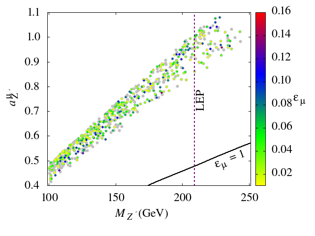
Figure 6: Allowed parameter space in $M_{Z^{\prime}}-a^{\mu}_{Z^{\prime}}$ plane with allowed values of the isospin violating parameter $\varepsilon_{\mu}$. Different values of $\varepsilon_{\mu}$ are indicated by different colour codes. The parameter space has been obtained by considering the current experimental results of $(g-2)_{\mu}$, $(g-2)_{e}$ (with negative value of $\Delta a_{e}$), latest data of $R_{K}$, $R_{K^{*}}$, leading angular observables ($P_{2}$ and $P^{\prime}_{5}$) of $B^{+}\to K^{+*}\mu^{+}\mu^{-}$ decay mode and ${B^{0}_{s}}-\bar{B^{0}_{s}}$ oscillation data. Further we imposed the CCFR data for neutrino trident production. Within the allowed parameter points the branching ratios for $B\to K^{(*)}\nu\bar{\nu}$ is found to be consistent with the experimental upper bound $1.6(2.7)\times 10^{-5}$ and remain one order of magnitude below this limit in the entire region of the parameter space of interest. If we relax the constraint from neutrino trident production cross section then there will be an enhancement of the allowed parameter space and which is reflected by the grey coloured region. The purple coloured vertical line represents the LEP collider bound on $M_{Z^{\prime}}$.

In Fig. 6 we present the parameter space which is allowed by experimental data considered in Sec. 5 and additionally is in agreement with the CCFR data for neutrino trident production and the limits on Br($B\to K^{(*)}\nu\bar{\nu}$). Expectedly the ${\rm SU(2)}_{L}$ invariant couplings are excluded by the CCFR data. This necessitates the introduction of non-trivial isospin violation in the $Z^{\prime}$ couplings parametrised by $\varepsilon_{l}\neq 1$. In Fig. 6 the allowed parameter points in the $M_{Z^{\prime}}-a^{\mu}_{Z^{\prime}}$ plane have values of $\varepsilon_{\mu}$ represented by different colours. The black line represents the CCFR exclusion limit for $\varepsilon_{\mu}=1$. As can be read off from the plot the region of parameter space consistent with $(g-2)_{\mu},B$-physics observable and CCFR require $\varepsilon_{\mu}<0.2.$ For the allowed parameter points the branching ratios for $B\to K^{(*)}\nu\bar{\nu}$ is found to be consistent with the experimental upper bound $1.6(2.7)\times 10^{-5}$ [93] and remain one order of magnitude below this limit in the entire region of the parameter space of interest.

A few comments about the direct collider bounds on the $Z^{\prime}$ model considered here is now in order. The most stringent collider bound on the effective framework arises from the LHC searched in the $pp\to Z\to 4\mu$ channel and is relevant in the range $5\lesssim M_{Z^{\prime}}\lesssim 70\,\mathrm{GeV}$ [125, 126, 114, 27] which is not of concern for the parameter space presented in Fig. 6. Given the coupling between the electron and $Z^{\prime}$ in the MFS the most relevant constraint from LEP [88] (indicated by purple coloured vertical dashed line in Fig. 6) exclude the parameter space below $M_{Z^{\prime}}<209$ GeV. The Fig. 6 clearly indicates that some of the sampled parameter points are able to survive all the constraints considered in this study provided an isospin violating coupling is assumed between the exotic $Z^{\prime}$ and the lepton doublets.

7 LKB measurement of $(g-2)_{e}$

Before we conclude we would like to remark on a recent measurement at Laboratoire Kastler Brossel (LKB) with rubidium atoms reported a new value for the fine structure constant [127]. Using this measurement, the SM prediction of $(g-2)_{e}$ shift, and is estimated to be $1.6\sigma$ lower with respect to the experimental value [4] with,

$$\Delta a_{e}=a_{e}^{\rm exp}-a_{e}^{\rm SM}=(4.8\pm 3.0)\times 10^{-13}.$$ (35)

A discussion about the minimal flavoured $Z^{\prime}$ scenario in view of this recent result is now in order.

(a)

(b)

(c)

(d)

Figure 7: Upper left panel: 1$\sigma$ allowed parameter space in $M_{Z^{\prime}}$ (in MeV) vs $a_{Z^{\prime}}$ plane satisfied by both the data of $(g-2)_{\mu}$ and $(g-2)_{e}$. Upper right panel: 1$\sigma$ allowed parameter space in $a_{Z^{\prime}}$ vs $b_{Z^{\prime}}$ (same for muon and electron) plane with the allowed values of $M_{Z^{\prime}}$ (in GeV) satisfied by both the data of $(g-2)_{\mu}$ and $(g-2)_{e}$. Lower left panel: 1$\sigma$ allowed parameter space in $a^{\mu}_{Z^{\prime}}$ vs $a^{e}_{Z^{\prime}}$ plane with allowed values of $M_{Z^{\prime}}$ (in GeV). Lower right panel: parameter space in $a^{\mu}_{Z^{\prime}}$ vs $a^{e}_{Z^{\prime}}$ plane with allowed values of $M_{Z^{\prime}}$ (in GeV) allowed by $\Delta a_{\mu}$ by Fermilab, result on $\Delta a_{e}$ given by LBL, latest data of $R_{K}$ published by LHCb collaboration, up to date values of $R_{K^{*}}$ for the both lower and central bin values of $q^{2}$ and leading angular observables of the decay mode $B^{+}\to K^{+*}\mu^{+}\mu^{-}$. The inset shows the region in $M_{Z^{\prime}}$ (in GeV) vs $\textsl{g}_{bs}$ plane allowed by the above mentioned experimental results.

1. With both positive value of $\Delta a_{e}$ and $\Delta a_{\mu}$ one can hope to explain both simultaneously in a scenario where both the electron and muon have identical vectorial coupling with the $Z^{\prime}$ as defined in Eq. 11. The corresponding $1\sigma$ allowed parameter space is shown in $M_{Z^{\prime}}$ vs $a_{Z^{\prime}}$ plane in the Fig. 7a. The preferred $M_{Z^{\prime}}$ in the MeV scale is too restricted to explain the LFUV in the $B$-meson sector.

2. A possibility is where both the electron and muon have vectorial as well as axial-vectorial coupling (of same strengths) with the $Z^{\prime}$. In such case the most recent data of $(g-2)_{e}$ with positive value of $\Delta a_{e}$ and the recent data of $(g-2)_{\mu}$ can be explained simultaneously. In Fig. 7b, $1\sigma$ allowed parameter space has been shown in $a_{Z^{\prime}}$ vs $b_{Z^{\prime}}$ plane for allowed values of $M_{Z^{\prime}}$. Again in this case also, the allowed values of independent parameters are restricted within very small values.

3. In the passing we note that the other possible four parameter model is where, $a^{\mu}_{Z^{\prime}}\neq 0$, $b^{\mu}_{Z^{\prime}}=0$ (for muon) but $a^{e}_{Z^{\prime}}=0$, $b^{e}_{Z^{\prime}}\neq 0$ (for electron), then it is not possible to explain both the $(g-2)_{\mu}$ and $(g-2)_{e}$ with positive value of $\Delta a_{e}$ simultaneously. Because, in such scenario $(g-2)_{e}$ with positive value of $\Delta a_{e}$ cannot be explained.

4. We further consider a four parameter scenario in which both the electron and muon have independent vectorial coupling with the $Z^{\prime}$. In Fig. 7c we have shown the 1$\sigma$ allowed parameter space satisfied by both the $(g-2)_{\mu}$ and $(g-2)_{e}$ with positive value of $\Delta a_{e}$. From this figure it is clear that the mass of the $Z^{\prime}$ can be increased substantially with respect to the previous scenarios making it more favourable to explain LFUV in the $B$-sector. We compute the LFUV observables $R_{K^{(*)}}$, ${B^{0}_{s}}-\bar{B^{0}_{s}}$ mass difference and leading angular observables of the decay mode $B^{+}\to K^{+*}\mu^{+}\mu^{-}$ with the motivation to find out the region of parameter space which satisfy the corresponding experimental results simultaneously. The result from our analysis is depicted in the Fig. 7d. The inset shows the corresponding allowed region in $M_{Z^{\prime}}$ (in GeV) vs $\textsl{g}_{bs}$ plane.

   We expectedly find that the identification of the most optimistic flavoured $Z^{\prime}$ model depends on the relative sign of the $\Delta a_{\mu}$ and $\Delta a_{e}$.

The numerical results presented here from our in-house implementation of the $B$-physics observables have been extensively validated with the results obtained from the publicly available package flavio [119]. We reproduce Fig. 5a, Fig. 5b, Fig. 6 and Fig. 7d using the package flavio. A detailed quantitative comparison of our results with flavio is presented in Appendix D.

8 Conclusion

A synergy of experimental results in measurement of $R_{K}$ (with $3.1\sigma$ deviation) and $R_{K^{*}}$ by LHCb collaboration, $(g-2)_{\mu}$ (with $4.2\sigma$ deviation) by Fermi Lab and $(g-2)_{e}$ provide a tantalizing hint of lepton flavour violation and hence Beyond Standard Model Physics in the flavour sector.

In this paper, instead of conforming to a specific UV complete scenario we survey the data driven phenomenological effective models with vectorial and axial-vectorial leptonic coupling for the $Z^{\prime}$. We systematically identify the minimal flavoured $Z^{\prime}$ model that can simultaneously explain these experimental evidences of lepton flavour universality violation while remaining in consonance with the correlated ${B^{0}_{s}}-\bar{B^{0}_{s}}$ oscillation. We explore the parameter space that is allowed by these observables taking into account the leading angular observables of the decay mode $B^{+}\to K^{+*}\mu^{+}\mu^{-}$.

From our systematic study we observe that the models are very sensitive to the relative sign between $\Delta a_{\mu}$ and $\Delta a_{e}$. For example, we find that a $Z^{\prime}$ that couple vectorially to moun while having an purely axial-vectorial coupling to electron can explain the data of anomalous magnetic moment of leptons (muon and electron). An off diagonal coupling to the quarks can simultaneously explain the $B$-physics observables for a weak scale $Z^{\prime}$. An increase in the resolution of measurement of the anomalous magnetic moment of lepton in the future will provide a handle in identifying specific scenarios of flavoured $Z^{\prime}$ models. On the other hand we find the minimal model with flavour specific vectorial coupling to the lepton suits the measurement of $\Delta a_{e}$ using the LKB data.

Interestingly the CCFR data for neutrino trident production cross section excludes an ${\rm SU(2)}_{L}$ invariant coupling between the exotic $Z^{\prime}$ and the leptonic doublets for models that simultaneously satisfy the $B$-physics and $(g-2)_{l}$ constraints. This implies the uncomfortable reality of an isospin violating couplings for the $Z^{\prime}$ along with flavour violation.

Acknowledgements We would like to give thank Chirashree Lahiri and Rohan Pramanick for computational and technical support. AS acknowledges the financial support from Department of Science and Technology, Government of India through SERB-NPDF scholarship with grant no.:PDF/2020/000245. TSR acknowledges Department of Science and Technology, Government of India, for support under grant agreement no.:ECR/2018/002192 [Early Career Research Award].

Appendix

Appendix A Relevant Wilson Coefficients for the $b\to sl^{+}l^{-}$ transitions

In this appendix we collect all the relevant Wilson Coefficients that are useful in constructing the observables related to the $b\to sl^{+}l^{-}$ transitions. The operator $\mathcal{O}_{10}$ does not evolve under QCD renormalisation and its coefficient is independent of energy scale $Q$ and can be expressed in the following way

$$C_{10}(Q)=-\frac{Y(x_{t})}{\sin^{2}\theta_{W}}+C^{\rm NP}_{10}\;,$$ (A-1)

where $\theta_{W}$ is the Weinberg angle. Unlike $C_{10}$, $C_{9}$ varies with energy scale and using the results of NLO QCD corrections to $C^{\rm eff}_{9}(Q)$ in the SM [128, 129] we can readily obtain this coefficient in the NP scenario under the naive dimensional regularisation (NDR) renormalisation scheme as

$$C_{9}^{\rm eff}(q^{2}) = C_{9}^{\rm NDR}\tilde{\eta}\left(\frac{q^{2}}{m^{2}_{b}}\right)+h\left(z,\frac{q^{2}}{m^{2}_{b}}\right)\left(3C_{1}+C_{2}+3C_{3}+C_{4}+3C_{5}+C_{6}\right)$$

$$-\frac{1}{2}h\left(1,\frac{q^{2}}{m^{2}_{b}}\right)\left(4C_{3}+4C_{4}+3C_{5}+C_{6}\right)-\frac{1}{2}h\left(0,\frac{q^{2}}{m^{2}_{b}}\right)\left(C_{3}+4C_{4}\right)$$

$$+\frac{2}{9}\left(3C_{3}+C_{4}+3C_{5}+C_{6}\right),$$

where,

$$C_{9}^{\rm NDR}=P_{0}^{\rm NDR}+\frac{Y(x_{t})}{\sin^{2}\theta_{W}}+C^{\rm NP}_{9}-4Z(x_{t})+P_{E}E(x_{t})\;.$$ (A-3)

The value of $P_{0}^{\rm NDR}(P_{E})$ is set at $2.60\pm 0.25$ [130] (${\cal O}(10^{-2})$ [129]). The function $Y(x_{t})$, $Z(x_{t})$ and $E(x_{t})$ are the usual Inami-Lim functions [129, 101]. The function $\tilde{\eta}$ (given in the Eq. A) represents single gluon corrections to the matrix element $\mathcal{O}_{9}$ and it takes the form [129]

$$\tilde{\eta}\left(\frac{q^{2}}{m^{2}_{b}}\right)=1+\frac{\alpha_{s}}{\pi}\omega\left(\frac{q^{2}}{m^{2}_{b}}\right),$$ (A-4)

where $\alpha_{s}$ is the QCD fine structure constant. The functional forms of $\omega$ and $h$ are given by [129]

$$\omega\left(\frac{q^{2}}{m^{2}_{b}}\right) = -{2\over 9}\pi^{2}-{4\over 3}{\rm Li}_{{}_{2}}\left(\frac{q^{2}}{m^{2}_{b}}\right)-{2\over 3}\ln\left(\frac{q^{2}}{m^{2}_{b}}\right)\ln\left(1-\frac{q^{2}}{m^{2}_{b}}\right)$$

$$-{5+4\frac{q^{2}}{m^{2}_{b}}\over 3\bigg{(}1+2\frac{q^{2}}{m^{2}_{b}}\bigg{)}}\ln\left(1-\frac{q^{2}}{m^{2}_{b}}\right)-{2\frac{q^{2}}{m^{2}_{b}}\bigg{(}1+\frac{q^{2}}{m^{2}_{b}}\bigg{)}\bigg{(}1-2\frac{q^{2}}{m^{2}_{b}}\bigg{)}\over 3\bigg{(}1-\frac{q^{2}}{m^{2}_{b}}\bigg{)}^{2}\bigg{(}1+2\frac{q^{2}}{m^{2}_{b}}\bigg{)}}\ln\left(\frac{q^{2}}{m^{2}_{b}}\right)$$

$$+{5+9\frac{q^{2}}{m^{2}_{b}}-6\left(\frac{q^{2}}{m^{2}_{b}}\right)^{2}\over 6\bigg{(}1-\frac{q^{2}}{m^{2}_{b}}\bigg{)}\bigg{(}1+2\frac{q^{2}}{m^{2}_{b}}\bigg{)}}\;,$$

and

$$h\left(z,\frac{q^{2}}{m^{2}_{b}}\right) = {8\over 27}-{8\over 9}\ln{m_{{}_{b}}\over\mu}-{8\over 9}\ln z+{16z^{2}m^{2}_{b}\over 9q^{2}}$$ (A-9)

$$-{4\over 9}\left(1+{2z^{2}m^{2}_{b}\over q^{2}}\right)\sqrt{\bigg{|}1-{4z^{2}m^{2}_{b}\over q^{2}}\bigg{|}}\left\{\begin{array}[]{ll}\ln\Bigg{|}{\sqrt{1-\frac{4z^{2}m^{2}_{b}}{q^{2}}}+1\over\sqrt{1-\frac{4z^{2}m^{2}_{b}}{q^{2}}}-1}\Bigg{|}-i\pi,&{\rm if}\>\frac{4z^{2}m^{2}_{b}}{q^{2}}<1\\ 2\arctan{1\over\sqrt{\frac{4z^{2}m^{2}_{b}}{q^{2}}-1}},&{\rm if}\>\frac{4z^{2}m^{2}_{b}}{q^{2}}>1\end{array}\right.\;.$$

Wilson Coefficients $C_{1}\ldots C_{6}$ are defined as [131]

$$C_{1}(M_{W}) = \frac{11}{2}\frac{\alpha_{s}(M_{W})}{4\pi}\;,$$ (A-10)

$$C_{2}(M_{W}) = 1-\frac{11}{6}\frac{\alpha_{s}(M_{W})}{4\pi}\;,$$ (A-11)

$$C_{3}(M_{W}) = -\frac{1}{3}C_{4}(M_{W})=-\frac{\alpha_{s}(M_{W})}{24\pi}=\widetilde{E}(x_{t})=E(x_{t})-\frac{2}{3}\;,$$ (A-12)

$$C_{5}(M_{W}) = -\frac{1}{3}C_{6}(M_{W})=-\frac{\alpha_{s}(M_{W})}{24\pi}=\widetilde{E}(x_{t})=E(x_{t})-\frac{2}{3}\;.$$ (A-13)

The formula of decay branching ratio of $B\to K^{(*)}l^{+}l^{-}$ consists of another effective Wilson Coefficient namely $C_{7}^{{\rm eff}}$ for which there is no NP contribution in our chosen scenario. Within the SM $C_{7}^{{\rm eff}}$ can be defined as [129]

$$C_{7}^{{\rm eff}} = -\frac{1}{2}\eta^{\frac{16}{23}}D^{\prime}(x_{t})-\frac{1}{2}\frac{8}{3}\left(\eta^{\frac{14}{23}}-\eta^{\frac{16}{23}}\right)E^{\prime}(x_{t})+C_{2}(M_{W})\sum_{i=1}^{8}h_{i}\eta^{a_{i}},$$ (A-14)

with

$$\eta=\frac{\alpha_{s}(M_{W})}{\alpha_{s}(m_{b})},~{}~{}~{}\alpha_{s}(m_{b})=\frac{\alpha_{s}(M_{Z})}{1-\frac{23}{3}\frac{\alpha_{s}(M_{Z})}{2\pi}\,\ln(M_{Z}/m_{b})}.$$ (A-15)

The values of $a_{i}$, $h_{i}$ and $\bar{h}_{i}$ can be obtained from [129]. $D^{\prime}(x_{t})$ and $E^{\prime}(x_{t})$ are the Inami-Lim functions [129, 101] that represent SM contributions (at the LO level) to the photonic and gluonic magnetic dipole moment operators.

Appendix B Form Factor for the $B\to K^{(*)}l^{+}l^{-}$ transitions

In this appendix we briefly summarise the $B\to K^{(*)}$ form factors related to the rare $B$-meson decays considered in our analysis.

B.1 Details of form factors for $B^{+}\to K^{+}l^{+}l^{-}$ transitions

The long-distance effects for hadronic dynamics of $B^{+}\to K^{+}l^{+}l^{-}$ decay is represented by the following matrix elements [132]

$$\langle K^{+}(p^{\prime})|\bar{s}\gamma^{\mu}b|B^{+}(p)\rangle = f_{+}(s)\,(p+p^{\prime})^{\mu}+[f_{0}(s)-f_{+}(s)]\,\frac{m^{2}_{B}-m^{2}_{K}}{q^{2}}q^{\mu}\,,$$ (B-16)

$$\langle K^{+}(p^{\prime})|\bar{s}\sigma^{\mu\nu}b|B^{+}(p)\rangle = i\frac{f_{T}(s)}{m_{B}+m_{K}}\left[(p+p^{\prime})^{\mu}q^{\nu}-q^{\mu}(p+p^{\prime})^{\nu}\right]\,.$$ (B-17)

Here, the form factors are $f_{+}$, $f_{0}$ and $f_{T}$. Further $q=p-p^{\prime}$ and $s=q^{2}/m^{2}_{B}$. $f_{0}$ terms drops out from the expression of differential decay width (see Eq. 20) due to smallness of lepton masses. Using the approach given in ref. [120] we implement the following expression for $f_{+}$,

$$f_{+}(q^{2})=\frac{1}{1-q^{2}/m_{+}^{2}}\left[\alpha_{0}+\alpha_{1}z(q^{2})+\alpha_{2}z^{2}(q^{2})+\frac{z^{3}(q^{2})}{3}(-\alpha_{1}+2\alpha_{2})\right],$$ (B-18)

with a simplified series expansion (SSE)

$$z(t)=\frac{\sqrt{t_{+}-t}-\sqrt{t_{+}-t_{0}}}{\sqrt{t_{+}-t}+\sqrt{t_{+}-t_{0}}}\,,$$ (B-19)

where, $t_{\pm}=(m_{B}\pm m_{K})^{2}$ and $t_{0}=t_{+}(1-\sqrt{1-t_{-}/t_{+}})$. The resonance mass is given by $m_{+}=m_{B}+0.046$ GeV. The values of the parameters $\alpha_{0}$, $\alpha_{1}$, and $\alpha_{2}$ as are given bellow [120]

$$\alpha_{0} =0.432\pm 0.011\,, \alpha_{1} =-0.664\pm 0.096\,, \alpha_{2} =-1.20\pm 0.69\,.$$ (B-20)

The corresponding expression for $f_{T}$ is extracted from the following ratio,

$$\frac{f_{T}(s)}{f_{+}(s)}=\frac{m_{B}+m_{K}}{m_{B}}\,.$$ (B-21)

This is independent of unknown hadronic quantities in the domain of interest [133, 134, 135, 136, 137, 138, 139].

B.2 Details of form factors for $B^{0}\to K^{0*}l^{+}l^{-}$ transitions

The matrix elements for the relevant operators for $B^{0}(p)\to K^{0*}(k)$ transitions in terms of momentum transfer ($q^{\mu}=p^{\mu}-k^{\mu}$) dependent form factors can be written as [106]

$$\langle K^{0*}(k)|\bar{s}\gamma_{\mu}(1-\gamma_{5})b|B^{0}(p)\rangle=-i\epsilon^{*}_{\mu}(m_{B}+m_{K^{*}})A_{1}(q^{2})+i(2p-q)_{\mu}(\epsilon^{*}\cdot q)\,\frac{A_{2}(q^{2})}{m_{B}+m_{K^{*}}}$$ (B-22)

$${}+iq_{\mu}(\epsilon^{*}\cdot q)\,\frac{2m_{K^{*}}}{q^{2}}\,\left[A_{3}(q^{2})-A_{0}(q^{2})\right]+\epsilon_{\mu\nu\rho\sigma}\epsilon^{*\nu}p^{\rho}k^{\sigma}\,\frac{2V(q^{2})}{m_{B}+m_{K^{*}}},\hskip 14.22636pt$$

and,

$$\langle K^{0*}(k)|\bar{s}\sigma_{\mu\nu}q^{\nu}(1+\gamma_{5})b|B^{0}(p)\rangle=i\epsilon_{\mu\nu\rho\sigma}\epsilon^{*\nu}p^{\rho}k^{\sigma}\,2T_{1}(q^{2})$$

$${}+T_{2}(q^{2})\left[\epsilon^{*}_{\mu}(m_{B}^{2}-m_{K^{*}}^{2})-(\epsilon^{*}\cdot q)\,(2p-q)_{\mu}\right]+T_{3}(q^{2})(\epsilon^{*}\cdot q)\left[q_{\mu}-\frac{q^{2}}{m_{B}^{2}-m_{K^{*}}^{2}}(2p-q)_{\mu}\right].$$

Here, $\epsilon_{\mu}$ represents polarization vector of the $K^{*}$. The form factors $A_{i}$ and $V$ are scale independent. On the other hand the $T_{i}$ depend on the renormalisation scale. The form factor in the light cone sum rules (LCSR) scheme can be generically written as [140]

$$F_{i}(q^{2})=P_{i}(q^{2})\sum_{k}\alpha_{k}^{i}\,\left[z^{*}(q^{2})-z^{*}(0)\right]^{k}\,,$$ (B-24)

with an SSE,

$$z^{*}(t)=\frac{\sqrt{t_{+}-t}-\sqrt{t_{+}-t_{0}}}{\sqrt{t_{+}-t}+\sqrt{t_{+}-t_{0}}}\;,$$ (B-25)

where, $t_{\pm}\equiv(m_{B}\pm m_{K^{*}})^{2}$ and $t_{0}\equiv t_{+}(1-\sqrt{1-t_{-}/t_{+}})$. Here, $P_{i}(q^{2})=(1-q^{2}/m_{R,i}^{2})^{-1}$ represents a simple pole corresponding to the first resonance in the spectrum. Appropriate resonance masses $m_{R,i}$ and the coefficients $\alpha^{i}_{k}$ can be extracted from [140].

Appendix C Transversity amplitudes

The expressions of the transversity amplitudes (up to corrections of $\mathcal{O}(\alpha_{s})$) in terms of appropriate Wilson Coefficients and form factors are given as follows [106]

$$A_{\perp L,R}=N\sqrt{2}\lambda^{1/2}\bigg{[}\left[C_{9}^{\text{eff}}\mp C_{10}\right]\frac{V(q^{2})}{m_{B}+m_{K^{*}}}+\frac{2m_{b}}{q^{2}}C_{7}^{\text{eff}}T_{1}(q^{2})\bigg{]},$$ (C-26)

$$A_{\parallel L,R}=-N\sqrt{2}(m_{B}^{2}-m_{K^{*}}^{2})\bigg{[}\left[C_{9}^{\text{eff}}\mp C_{10}\right]\frac{A_{1}(q^{2})}{m_{B}-m_{K^{*}}}+\frac{2m_{b}}{q^{2}}C_{7}^{\text{eff}}T_{2}(q^{2})\bigg{]},$$ (C-27)

$$A_{0L,R}=-\frac{N}{2m_{K^{*}}\sqrt{q^{2}}}\bigg{\{}\left[C_{9}^{\text{eff}}\mp C_{10}\right]\bigg{[}(m_{B}^{2}-m_{K^{*}}^{2}-q^{2})(m_{B}+m_{K^{*}})A_{1}(q^{2})-\lambda\frac{A_{2}(q^{2})}{m_{B}+m_{K^{*}}}\bigg{]}$$

$$+{2m_{b}}C_{7}^{\text{eff}}\bigg{[}(m_{B}^{2}+3m_{K^{*}}^{2}-q^{2})T_{2}(q^{2})-\frac{\lambda}{m_{B}^{2}-m_{K^{*}}^{2}}T_{3}(q^{2})\bigg{]}\bigg{\}},$$ (C-28)

$$A_{t}=\frac{N}{\sqrt{q^{2}}}\lambda^{1/2}2C_{10}A_{0}(q^{2}),$$ (C-29)

with

$$N=V_{tb}^{\vphantom{*}}V_{ts}^{*}\left[\frac{G_{F}^{2}\alpha^{2}_{\rm em}}{3\cdot 2^{10}\pi^{5}m_{B}^{3}}q^{2}\lambda^{1/2}\beta_{l}\right]^{1/2},$$ (C-30)

where $\lambda=m_{B}^{4}+m_{K^{*}}^{4}+q^{4}-2(m_{B}^{2}m_{K^{*}}^{2}+m_{K^{*}}^{2}q^{2}+m_{B}^{2}q^{2})$ and $\beta_{l}=\sqrt{1-4m_{l}^{2}/q^{2}}$. Moreover, $L$ and $R$ refer to the chirality of the leptonic current. Here the particular amplitude $A_{t}$ is related to the time-like component of the virtual $K^{*}$, and it does not contribute in the case of massless leptons. Therefore, it can be neglected if the lepton mass is small in comparison to the mass of the lepton pair.

Appendix D Relative comparison with flavio

In this appendix we present a detailed comparison of numerical results obtained from our in-house implementation and the publicly available package flavio [119].

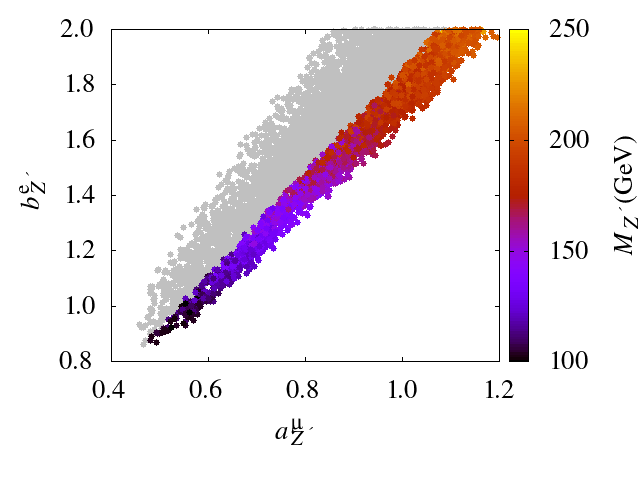
(a)

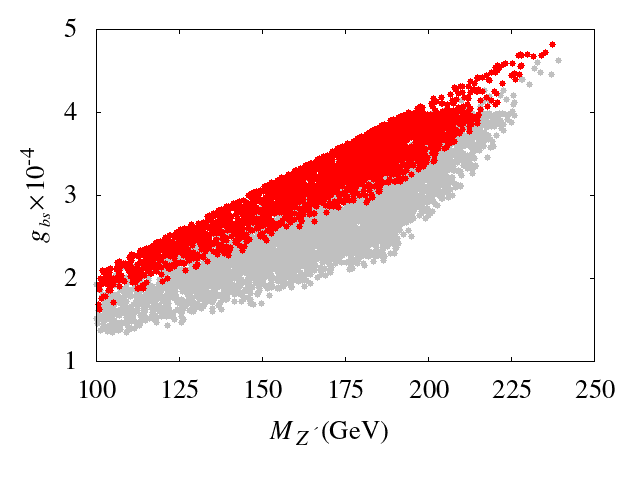
(b)

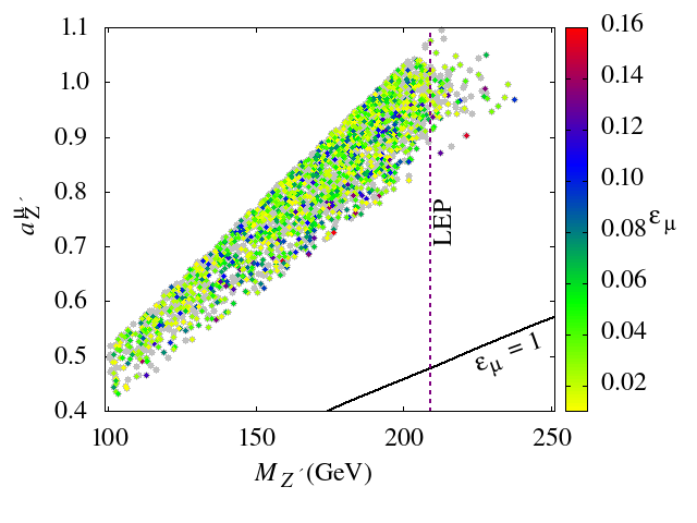
(c)

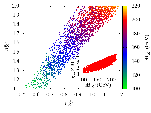
(d)

Figure 8: The plots are generated from the results of the package flavio. Similar plots have been presented in Fig. 5, Fig. 6 and Fig. 7d respectively, but obtained from the results of our in-house code.

Using the package flavio the relevant plots have been generated and presented in Figs. 8a, 8b, 8c and 8d. These may be compared with Figs. 5a, 5b, 6 and 7d respectively. Admittedly there is numerical differences which remains below $\sim 7\%$ in the region of interest. However, the qualitative nature of the results obtained remain consistent with each other.

References

- [1] Muon g-2 collaboration, B. Abi et al., Measurement of the Positive Muon Anomalous Magnetic Moment to 0.46 ppm, Phys. Rev. Lett. 126 (2021) 141801, [2104.03281].
- [2] S. Borsanyi et al., Leading hadronic contribution to the muon magnetic moment from lattice QCD, Nature 593 (2021) 51–55, [2002.12347].
- [3] R. H. Parker, C. Yu, W. Zhong, B. Estey and H. Müller, Measurement of the fine-structure constant as a test of the Standard Model, Science 360 (2018) 191, [1812.04130].
- [4] D. Hanneke, S. Fogwell and G. Gabrielse, New Measurement of the Electron Magnetic Moment and the Fine Structure Constant, Phys. Rev. Lett. 100 (2008) 120801, [0801.1134].
- [5] M. Shifman, A. Vainshtein and V. Zakharov, Qcd and resonance physics. theoretical foundations, Nuclear Physics B 147 (1979) 385–447.
- [6] P. Colangelo and A. Khodjamirian, QCD sum rules, a modern perspective, hep-ph/0010175.
- [7] S. Descotes-Genon, L. Hofer, J. Matias and J. Virto, Global analysis of anomalies, JHEP 06 (2016) 092, [1510.04239].
- [8] M. Bordone, G. Isidori and A. Pattori, On the Standard Model predictions for and , Eur. Phys. J. C 76 (2016) 440, [1605.07633].
- [9] B. Capdevila, A. Crivellin, S. Descotes-Genon, J. Matias and J. Virto, Patterns of New Physics in transitions in the light of recent data, JHEP 01 (2018) 093, [1704.05340].
- [10] LHCb collaboration, R. Aaij et al., Test of lepton universality in beauty-quark decays, Nature Phys. 18 (2022) 277–282, [2103.11769].
- [11] LHCb collaboration, R. Aaij et al., Test of lepton universality with decays, JHEP 08 (2017) 055, [1705.05802].
- [12] R. Gauld, F. Goertz and U. Haisch, On minimal explanations of the anomaly, Phys. Rev. D 89 (2014) 015005, [1308.1959].
- [13] S. L. Glashow, D. Guadagnoli and K. Lane, Lepton Flavor Violation in Decays?, Phys. Rev. Lett. 114 (2015) 091801, [1411.0565].
- [14] B. Bhattacharya, A. Datta, D. London and S. Shivashankara, Simultaneous Explanation of the and Puzzles, Phys. Lett. B 742 (2015) 370–374, [1412.7164].
- [15] A. Crivellin, G. D’Ambrosio and J. Heeck, Explaining , and in a two-Higgs-doublet model with gauged , Phys. Rev. Lett. 114 (2015) 151801, [1501.00993].
- [16] A. Crivellin, L. Hofer, J. Matias, U. Nierste, S. Pokorski and J. Rosiek, Lepton-flavour violating decays in generic models, Phys. Rev. D 92 (2015) 054013, [1504.07928].
- [17] A. Celis, J. Fuentes-Martin, M. Jung and H. Serodio, Family nonuniversal Z’ models with protected flavor-changing interactions, Phys. Rev. D 92 (2015) 015007, [1505.03079].
- [18] D. Aristizabal Sierra, F. Staub and A. Vicente, Shedding light on the anomalies with a dark sector, Phys. Rev. D 92 (2015) 015001, [1503.06077].
- [19] G. Bélanger, C. Delaunay and S. Westhoff, A Dark Matter Relic From Muon Anomalies, Phys. Rev. D 92 (2015) 055021, [1507.06660].
- [20] B. Gripaios, M. Nardecchia and S. A. Renner, Linear flavour violation and anomalies in B physics, JHEP 06 (2016) 083, [1509.05020].
- [21] B. Allanach, F. S. Queiroz, A. Strumia and S. Sun, models for the LHCb and muon anomalies, Phys. Rev. D 93 (2016) 055045, [1511.07447].
- [22] K. Fuyuto, W.-S. Hou and M. Kohda, Z’ -induced FCNC decays of top, beauty, and strange quarks, Phys. Rev. D 93 (2016) 054021, [1512.09026].
- [23] C.-W. Chiang, X.-G. He and G. Valencia, model for b→s flavor anomalies, Phys. Rev. D 93 (2016) 074003, [1601.07328].
- [24] S. M. Boucenna, A. Celis, J. Fuentes-Martin, A. Vicente and J. Virto, Non-abelian gauge extensions for B-decay anomalies, Phys. Lett. B 760 (2016) 214–219, [1604.03088].
- [25] S. M. Boucenna, A. Celis, J. Fuentes-Martin, A. Vicente and J. Virto, Phenomenology of an model with lepton-flavour non-universality, JHEP 12 (2016) 059, [1608.01349].
- [26] A. Celis, W.-Z. Feng and M. Vollmann, Dirac dark matter and with gauge symmetry, Phys. Rev. D 95 (2017) 035018, [1608.03894].
- [27] W. Altmannshofer, S. Gori, S. Profumo and F. S. Queiroz, Explaining dark matter and B decay anomalies with an model, JHEP 12 (2016) 106, [1609.04026].
- [28] B. Bhattacharya, A. Datta, J.-P. Guévin, D. London and R. Watanabe, Simultaneous Explanation of the and Puzzles: a Model Analysis, JHEP 01 (2017) 015, [1609.09078].
- [29] A. Crivellin, J. Fuentes-Martin, A. Greljo and G. Isidori, Lepton Flavor Non-Universality in B decays from Dynamical Yukawas, Phys. Lett. B 766 (2017) 77–85, [1611.02703].
- [30] D. Bečirević, O. Sumensari and R. Zukanovich Funchal, Lepton flavor violation in exclusive decays, Eur. Phys. J. C 76 (2016) 134, [1602.00881].
- [31] I. Garcia Garcia, LHCb anomalies from a natural perspective, JHEP 03 (2017) 040, [1611.03507].
- [32] D. Bhatia, S. Chakraborty and A. Dighe, Neutrino mixing and anomaly in U(1)X models: a bottom-up approach, JHEP 03 (2017) 117, [1701.05825].
- [33] P. Ko, T. Nomura and H. Okada, Explaining anomaly by radiatively induced coupling in gauge symmetry, Phys. Rev. D 95 (2017) 111701, [1702.02699].
- [34] C.-H. Chen and T. Nomura, Penguin and -meson anomalies in a gauged , Phys. Lett. B 777 (2018) 420–427, [1707.03249].
- [35] S. Baek, Dark matter contribution to anomaly in local model, Phys. Lett. B 781 (2018) 376–382, [1707.04573].
- [36] S. F. King, Flavourful models for , JHEP 08 (2017) 019, [1706.06100].
- [37] S. F. King, and the origin of Yukawa couplings, JHEP 09 (2018) 069, [1806.06780].
- [38] S. Dasgupta, U. K. Dey, T. Jha and T. S. Ray, Status of a flavor-maximal nonminimal universal extra dimension model, Phys. Rev. D 98 (2018) 055006, [1801.09722].
- [39] A. Biswas and A. Shaw, Reconciling dark matter, anomalies and in an scenario, JHEP 05 (2019) 165, [1903.08745].
- [40] S. Dwivedi, D. Kumar Ghosh, A. Falkowski and N. Ghosh, Associated production in the flavorful scenario for , Eur. Phys. J. C 80 (2020) 263, [1908.03031].
- [41] A. E. Cárcamo Hernández, S. F. King, H. Lee and S. J. Rowley, Is it possible to explain the muon and electron in a model?, Phys. Rev. D 101 (2020) 115016, [1910.10734].
- [42] A. Bodas, R. Coy and S. J. D. King, Solving the electron and muon anomalies in models, Eur. Phys. J. C 81 (2021) 1065, [2102.07781].
- [43] A. Biswas and S. Khan, (g 2)e,μ and strongly interacting dark matter with collider implications, JHEP 07 (2022) 037, [2112.08393].
- [44] G. Hiller and M. Schmaltz, and future physics beyond the standard model opportunities, Phys. Rev. D 90 (2014) 054014, [1408.1627].
- [45] S. Biswas, D. Chowdhury, S. Han and S. J. Lee, Explaining the lepton non-universality at the LHCb and CMS within a unified framework, JHEP 02 (2015) 142, [1409.0882].
- [46] B. Gripaios, M. Nardecchia and S. A. Renner, Composite leptoquarks and anomalies in -meson decays, JHEP 05 (2015) 006, [1412.1791].
- [47] S. Sahoo and R. Mohanta, Scalar leptoquarks and the rare meson decays, Phys. Rev. D 91 (2015) 094019, [1501.05193].
- [48] D. Bečirević, S. Fajfer and N. Košnik, Lepton flavor nonuniversality in b→s+- processes, Phys. Rev. D 92 (2015) 014016, [1503.09024].
- [49] R. Alonso, B. Grinstein and J. Martin Camalich, Lepton universality violation and lepton flavor conservation in -meson decays, JHEP 10 (2015) 184, [1505.05164].
- [50] L. Calibbi, A. Crivellin and T. Ota, Effective Field Theory Approach to , and with Third Generation Couplings, Phys. Rev. Lett. 115 (2015) 181801, [1506.02661].
- [51] W. Huang and Y.-L. Tang, Flavor anomalies at the LHC and the R-parity violating supersymmetric model extended with vectorlike particles, Phys. Rev. D 92 (2015) 094015, [1509.08599].
- [52] H. Päs and E. Schumacher, Common origin of and neutrino masses, Phys. Rev. D 92 (2015) 114025, [1510.08757].
- [53] M. Bauer and M. Neubert, Minimal Leptoquark Explanation for the , , and Anomalies, Phys. Rev. Lett. 116 (2016) 141802, [1511.01900].
- [54] S. Fajfer and N. Košnik, Vector leptoquark resolution of and puzzles, Phys. Lett. B 755 (2016) 270–274, [1511.06024].
- [55] R. Barbieri, G. Isidori, A. Pattori and F. Senia, Anomalies in -decays and flavour symmetry, Eur. Phys. J. C 76 (2016) 67, [1512.01560].
- [56] S. Sahoo and R. Mohanta, Lepton flavor violating B meson decays via a scalar leptoquark, Phys. Rev. D 93 (2016) 114001, [1512.04657].
- [57] I. Doršner, S. Fajfer, A. Greljo, J. F. Kamenik and N. Košnik, Physics of leptoquarks in precision experiments and at particle colliders, Phys. Rept. 641 (2016) 1–68, [1603.04993].
- [58] S. Sahoo and R. Mohanta, Effects of scalar leptoquark on semileptonic decays, New J. Phys. 18 (2016) 093051, [1607.04449].
- [59] D. Das, C. Hati, G. Kumar and N. Mahajan, Towards a unified explanation of , and anomalies in a left-right model with leptoquarks, Phys. Rev. D 94 (2016) 055034, [1605.06313].
- [60] C.-H. Chen, T. Nomura and H. Okada, Explanation of and muon , and implications at the LHC, Phys. Rev. D 94 (2016) 115005, [1607.04857].
- [61] D. Bečirević, N. Košnik, O. Sumensari and R. Zukanovich Funchal, Palatable Leptoquark Scenarios for Lepton Flavor Violation in Exclusive modes, JHEP 11 (2016) 035, [1608.07583].
- [62] D. Bečirević, S. Fajfer, N. Košnik and O. Sumensari, Leptoquark model to explain the -physics anomalies, and , Phys. Rev. D 94 (2016) 115021, [1608.08501].
- [63] S. Sahoo, R. Mohanta and A. K. Giri, Explaining the and anomalies with vector leptoquarks, Phys. Rev. D 95 (2017) 035027, [1609.04367].
- [64] R. Barbieri, C. W. Murphy and F. Senia, B-decay Anomalies in a Composite Leptoquark Model, Eur. Phys. J. C 77 (2017) 8, [1611.04930].
- [65] P. Cox, A. Kusenko, O. Sumensari and T. T. Yanagida, SU(5) Unification with TeV-scale Leptoquarks, JHEP 03 (2017) 035, [1612.03923].
- [66] E. Ma, D. P. Roy and S. Roy, Gauged L(mu) - L(tau) with large muon anomalous magnetic moment and the bimaximal mixing of neutrinos, Phys. Lett. B 525 (2002) 101–106, [hep-ph/0110146].
- [67] S. Baek, N. G. Deshpande, X. G. He and P. Ko, Muon anomalous g-2 and gauged L(muon) - L(tau) models, Phys. Rev. D 64 (2001) 055006, [hep-ph/0104141].
- [68] J. Heeck and W. Rodejohann, Gauged Symmetry at the Electroweak Scale, Phys. Rev. D 84 (2011) 075007, [1107.5238].
- [69] K. Harigaya, T. Igari, M. M. Nojiri, M. Takeuchi and K. Tobe, Muon g-2 and LHC phenomenology in the gauge symmetric model, JHEP 03 (2014) 105, [1311.0870].
- [70] W. Altmannshofer, C.-Y. Chen, P. S. Bhupal Dev and A. Soni, Lepton flavor violating Z’ explanation of the muon anomalous magnetic moment, Phys. Lett. B 762 (2016) 389–398, [1607.06832].
- [71] A. Biswas, S. Choubey and S. Khan, Neutrino Mass, Dark Matter and Anomalous Magnetic Moment of Muon in a Model, JHEP 09 (2016) 147, [1608.04194].
- [72] A. Biswas, S. Choubey and S. Khan, FIMP and Muon () in a U Model, JHEP 02 (2017) 123, [1612.03067].
- [73] H. Banerjee, P. Byakti and S. Roy, Supersymmetric gauged U(1) model for neutrinos and the muon anomaly, Phys. Rev. D 98 (2018) 075022, [1805.04415].
- [74] D. Huang, A. P. Morais and R. Santos, Anomalies in -meson decays and the muon from dark loops, Phys. Rev. D 102 (2020) 075009, [2007.05082].
- [75] S. Q. Dinh and H. M. Tran, Muon g-2 and semileptonic B decays in the Bélanger-Delaunay-Westhoff model with gauge kinetic mixing, Phys. Rev. D 104 (2021) 115009, [2011.07182].
- [76] M. Chakraborti, S. Heinemeyer and I. Saha, Improved measurements and wino/higgsino dark matter, Eur. Phys. J. C 81 (2021) 1069, [2103.13403].
- [77] M. Chakraborti, S. Heinemeyer and I. Saha, The new “MUON G-2” result and supersymmetry, Eur. Phys. J. C 81 (2021) 1114, [2104.03287].
- [78] G. Arcadi, L. Calibbi, M. Fedele and F. Mescia, Muon and -anomalies from Dark Matter, Phys. Rev. Lett. 127 (2021) 061802, [2104.03228].
- [79] J. S. Alvarado, S. F. Mantilla, R. Martinez and F. Ochoa, A non-universal extension to the Standard Model to study the meson anomaly and muon , 2105.04715.
- [80] J. Davighi, Anomalous Z’ bosons for anomalous B decays, JHEP 08 (2021) 101, [2105.06918].
- [81] L. Darmé, M. Fedele, K. Kowalska and E. M. Sessolo, Flavour anomalies and the muon g 2 from feebly interacting particles, JHEP 03 (2022) 085, [2106.12582].
- [82] J.-P. Lee, with vector unparticles, 2106.12795.
- [83] A. Greljo, Y. Soreq, P. Stangl, A. E. Thomsen and J. Zupan, Muonic force behind flavor anomalies, JHEP 04 (2022) 151, [2107.07518].
- [84] X. Wang, Muon (g 2) and flavor puzzles in the U(1)X-gauged leptoquark model, JHEP 08 (2022) 243, [2108.01279].
- [85] M. F. Navarro and S. F. King, Fermiophobic model for simultaneously explaining the muon anomalies RK(*) and (g-2), Phys. Rev. D 105 (2022) 035015, [2109.08729].
- [86] R. Bause, G. Hiller, T. Höhne, D. F. Litim and T. Steudtner, B-anomalies from flavorful U(1)′ extensions, safely, Eur. Phys. J. C 82 (2022) 42, [2109.06201].
- [87] P. Ko, T. Nomura and H. Okada, Muon , anomalies, and leptophilic dark matter in gauge symmetry, 2110.10513.
- [88] Particle Data Group collaboration, P. A. Zyla et al., Review of Particle Physics, PTEP 2020 (2020) 083C01.
- [89] LHCb collaboration, R. Aaij et al., Angular Analysis of the Decay, Phys. Rev. Lett. 126 (2021) 161802, [2012.13241].
- [90] LHCb collaboration, R. Aaij et al., Search for the Rare Decays and , Phys. Rev. Lett. 124 (2020) 211802, [2003.03999].
- [91] LHCb collaboration, R. Aaij et al., Measurement of the branching fraction at low dilepton mass, JHEP 05 (2013) 159, [1304.3035].
- [92] LHCb collaboration, R. Aaij et al., Test of lepton universality using decays, Phys. Rev. Lett. 113 (2014) 151601, [1406.6482].
- [93] Belle collaboration, J. Grygier et al., Search for decays with semileptonic tagging at Belle, Phys. Rev. D 96 (2017) 091101, [1702.03224].
- [94] CCFR collaboration, S. R. Mishra et al., Neutrino tridents and W Z interference, Phys. Rev. Lett. 66 (1991) 3117–3120.
- [95] S. N. Gninenko and N. V. Krasnikov, The Muon anomalous magnetic moment and a new light gauge boson, Phys. Lett. B 513 (2001) 119, [hep-ph/0102222].
- [96] T. Aoyama et al., The anomalous magnetic moment of the muon in the Standard Model, Phys. Rept. 887 (2020) 1–166, [2006.04822].
- [97] T. Aoyama, T. Kinoshita and M. Nio, Revised and Improved Value of the QED Tenth-Order Electron Anomalous Magnetic Moment, Phys. Rev. D 97 (2018) 036001, [1712.06060].
- [98] G. Hiller, C. Hormigos-Feliu, D. F. Litim and T. Steudtner, Anomalous magnetic moments from asymptotic safety, Phys. Rev. D 102 (2020) 071901, [1910.14062].
- [99] G. Hiller and F. Kruger, More model-independent analysis of processes, Phys. Rev. D 69 (2004) 074020, [hep-ph/0310219].
- [100] G. Isidori, S. Nabeebaccus and R. Zwicky, QED corrections in at the double-differential level, JHEP 12 (2020) 104, [2009.00929].
- [101] G. Buchalla, A. J. Buras and M. E. Lautenbacher, Weak decays beyond leading logarithms, Rev. Mod. Phys. 68 (1996) 1125–1144, [hep-ph/9512380].
- [102] A. J. Buras, F. De Fazio, J. Girrbach and M. V. Carlucci, The Anatomy of Quark Flavour Observables in 331 Models in the Flavour Precision Era, JHEP 02 (2013) 023, [1211.1237].
- [103] W. Altmannshofer and D. M. Straub, New physics in transitions after LHC run 1, Eur. Phys. J. C 75 (2015) 382, [1411.3161].
- [104] C. Bobeth, G. Hiller and G. Piranishvili, CP Asymmetries in bar and Untagged , Decays at NLO, JHEP 07 (2008) 106, [0805.2525].
- [105] J. Matias, F. Mescia, M. Ramon and J. Virto, Complete Anatomy of and its angular distribution, JHEP 04 (2012) 104, [1202.4266].
- [106] W. Altmannshofer, P. Ball, A. Bharucha, A. J. Buras, D. M. Straub and M. Wick, Symmetries and Asymmetries of Decays in the Standard Model and Beyond, JHEP 01 (2009) 019, [0811.1214].
- [107] A. J. Buras, M. Jamin and P. H. Weisz, Leading and Next-to-leading QCD Corrections to Parameter and Mixing in the Presence of a Heavy Top Quark, Nucl. Phys. B 347 (1990) 491–536.
- [108] J. Urban, F. Krauss, U. Jentschura and G. Soff, Next-to-leading order QCD corrections for the B0 anti-B0 mixing with an extended Higgs sector, Nucl. Phys. B 523 (1998) 40–58, [hep-ph/9710245].
- [109] A. Lenz and G. Tetlalmatzi-Xolocotzi, Model-independent bounds on new physics effects in non-leptonic tree-level decays of B-mesons, JHEP 07 (2020) 177, [1912.07621].
- [110] A. J. Buras and J. Girrbach, Complete NLO QCD Corrections for Tree Level Delta F = 2 FCNC Processes, JHEP 03 (2012) 052, [1201.1302].
- [111] A. J. Buras, S. Jager and J. Urban, Master formulae for Delta F=2 NLO QCD factors in the standard model and beyond, Nucl. Phys. B 605 (2001) 600–624, [hep-ph/0102316].
- [112] LHCb collaboration, R. Aaij et al., Measurement of -Averaged Observables in the Decay, Phys. Rev. Lett. 125 (2020) 011802, [2003.04831].
- [113] S. Descotes-Genon, T. Hurth, J. Matias and J. Virto, Optimizing the basis of observables in the full kinematic range, JHEP 05 (2013) 137, [1303.5794].
- [114] W. Altmannshofer, S. Gori, M. Pospelov and I. Yavin, Neutrino Trident Production: A Powerful Probe of New Physics with Neutrino Beams, Phys. Rev. Lett. 113 (2014) 091801, [1406.2332].
- [115] W. Altmannshofer, S. Gori, J. Martín-Albo, A. Sousa and M. Wallbank, Neutrino Tridents at DUNE, Phys. Rev. D 100 (2019) 115029, [1902.06765].
- [116] T. Li, Q.-F. Xiang, Q.-S. Yan, X. Zhang and H. Zhou, Isospin-violating dark matter in a U(1)’ model inspired by , Phys. Rev. D 101 (2020) 035016, [1908.00423].
- [117] M. T. Frandsen, F. Kahlhoefer, S. Sarkar and K. Schmidt-Hoberg, Direct detection of dark matter in models with a light Z’, JHEP 09 (2011) 128, [1107.2118].
- [118] T. Li, Q. Xiang, X. Yin and H. Zhou, Generic U(1)X models inspired from SO(10), Phys. Rev. D 106 (2022) 075010, [2201.03878].
- [119] D. M. Straub, flavio: a Python package for flavour and precision phenomenology in the Standard Model and beyond, 1810.08132.
- [120] A. J. Buras, J. Girrbach-Noe, C. Niehoff and D. M. Straub, decays in the Standard Model and beyond, JHEP 02 (2015) 184, [1409.4557].
- [121] G. Bellini et al., Precision measurement of the 7Be solar neutrino interaction rate in Borexino, Phys. Rev. Lett. 107 (2011) 141302, [1104.1816].
- [122] Borexino collaboration, G. Bellini et al., Final results of Borexino Phase-I on low energy solar neutrino spectroscopy, Phys. Rev. D 89 (2014) 112007, [1308.0443].
- [123] Borexino collaboration, M. Agostini et al., First Simultaneous Precision Spectroscopy of , 7Be, and Solar Neutrinos with Borexino Phase-II, Phys. Rev. D 100 (2019) 082004, [1707.09279].
- [124] M. Lindner, F. S. Queiroz, W. Rodejohann and X.-J. Xu, Neutrino-electron scattering: general constraints on and dark photon models, JHEP 05 (2018) 098, [1803.00060].
- [125] A. Falkowski, S. F. King, E. Perdomo and M. Pierre, Flavourful portal for vector-like neutrino Dark Matter and , JHEP 08 (2018) 061, [1803.04430].
- [126] W. Altmannshofer, S. Gori, M. Pospelov and I. Yavin, Quark flavor transitions in models, Phys. Rev. D 89 (2014) 095033, [1403.1269].
- [127] L. Morel, Z. Yao, P. Cladé and S. Guellati-Khélifa, Determination of the fine-structure constant with an accuracy of 81 parts per trillion, Nature 588 (2020) 61–65.
- [128] M. Misiak, The and decays with next-to-leading logarithmic QCD corrections, Nucl. Phys. B 393 (1993) 23–45.
- [129] A. J. Buras and M. Munz, Effective Hamiltonian for B — X(s) e+ e- beyond leading logarithms in the NDR and HV schemes, Phys. Rev. D 52 (1995) 186–195, [hep-ph/9501281].
- [130] A. J. Buras, A. Poschenrieder, M. Spranger and A. Weiler, The Impact of universal extra dimensions on B — X(s) gamma, B — X(s) gluon, B — X(s) mu+ mu-, K(L) — pi0 e+ e- and epsilon-prime / epsilon, Nucl. Phys. B 678 (2004) 455–490, [hep-ph/0306158].
- [131] A. J. Buras, M. E. Lautenbacher, M. Misiak and M. Munz, Direct CP violation in K(L) — pi0 e+ e- beyond leading logarithms, Nucl. Phys. B 423 (1994) 349–383, [hep-ph/9402347].
- [132] M. Bartsch, M. Beylich, G. Buchalla and D. N. Gao, Precision Flavour Physics with and , JHEP 11 (2009) 011, [0909.1512].
- [133] J. Charles, A. Le Yaouanc, L. Oliver, O. Pene and J. C. Raynal, Heavy to light form-factors in the heavy mass to large energy limit of QCD, Phys. Rev. D 60 (1999) 014001, [hep-ph/9812358].
- [134] M. Beneke and T. Feldmann, Symmetry breaking corrections to heavy to light B meson form-factors at large recoil, Nucl. Phys. B 592 (2001) 3–34, [hep-ph/0008255].
- [135] M. B. Wise, Chiral perturbation theory for hadrons containing a heavy quark, Phys. Rev. D 45 (1992) R2188.
- [136] G. Burdman and J. F. Donoghue, Union of chiral and heavy quark symmetries, Phys. Lett. B 280 (1992) 287–291.
- [137] A. F. Falk and B. Grinstein, Anti-B — Anti-K e+ e- in Chiral Perturbation Theory, Nucl. Phys. B 416 (1994) 771–785, [hep-ph/9306310].
- [138] R. Casalbuoni, A. Deandrea, N. Di Bartolomeo, R. Gatto, F. Feruglio and G. Nardulli, Phenomenology of heavy meson chiral Lagrangians, Phys. Rept. 281 (1997) 145–238, [hep-ph/9605342].
- [139] G. Buchalla and G. Isidori, Nonperturbative effects in for large dilepton invariant mass, Nucl. Phys. B 525 (1998) 333–349, [hep-ph/9801456].
- [140] A. Bharucha, D. M. Straub and R. Zwicky, in the Standard Model from light-cone sum rules, JHEP 08 (2016) 098, [1503.05534].