Radiative corrections to elastic muon-proton scattering
at low momentum transfers

Abstract

We systematically calculate the radiative corrections of order $\alpha/\pi$ to elastic muon-proton scattering at low momentum transfers. These include vacuum polarization, photon-loop form factors of the muon and the proton, two-photon exchange corrections and soft photon radiation. In particular, we discuss these corrections for the kinematics of the upcomimg AMBER experiment with a $100\,$GeV muon beam energy. It is found that for the ratio to the Born cross section, only the minor terms from the photon-loop form factors of the proton and two-photon exchange depend on the proton structure predetermined by the strong interactions. Since a prominent role among the radiative corrections is played by soft photon radiation, the calculation of the bremsstrahlung process $\mu p\to\mu p\gamma$ should be extended beyond the soft photon approximation and tailored to the specific experimental conditions.

I Introduction

Elastic muon-proton scattering at low momentum transfers offers an alternative method to measure the proton charge radius $r_{p}$, which is a fundamental quantity in the theory of the strong interactions. It is defined here by the slope of the proton charge form factor $G_{E,p}(Q)$ at zero momentum transfer $r_{p}^{2}=-6\,{dG_{E,p}(Q)}/{dQ^{2}}|_{Q=0}$, with $Q^{2}$ the invariant four-momentum transfer squared. Any deviation from the value measured in electron-proton scattering would challenge the concept of lepton-flavor universality, which is a cornerstone of the so successful Standard Model of particle physics, that has been challenged in recent experiments on certain decay modes of B mesons, see Ref. Bifani:2018zmi for a recent review. Two experiments are pursuing such proton radius measurements, namely MUSE at PSI Downie:2014qna and AMBER at CERN Adams:2018pwt . Both experiments were triggered by the so-called “proton radius puzzle”, see e.g. Ref. Pohl:2013yb , but it must be said that most recent determinations of the proton radius from electron-proton scattering and the Lamb shift in electronic hydrogen are in favor of the so-called small radius, $r_{p}\simeq 0.84\,$fm, as collected in Tab. 1. The small value is further supported by a dispersion-theoretical analysis of all existing scattering and annihilation data in the space-like and the time-like region Lin:2021xrc , as also shown in the table. The underlying dispersive framework and the history of proton radius extractions based on dispersion relations (DRs) are discussed in detail in Ref. Lin:2021umz . Still, an independent extraction from $\mu^{\mp}p$ scattering would be highly welcome, further complementing the groundbreaking work on the Lamb shift in muonic hydrogen Pohl:2010zza , which essentially initiated the whole proton radius discussion.

Table 1: Modern precision extractions of the proton charge radius $r_{p}$ from the Lamb shift in electronic hydrogen and electron-proton scattering as well as dispersion theory.

$r_{p}$ [fm]	year	method	Ref.
0.877(13)	2018	H Lamb shift	Fleurbaey:2018fih
0.833(10)	2019	H Lamb shift	Bezginov:2019mdi
0.8482(38)	2020	H Lamb shift	Griffin:2020
0.8584(51)	2021	H Lamb shift	Brandt:2021yor
0.831(7)(12)	2019	$ep$ scattering	Jlab
0.840(3)(2)	2022	disp. theory	Lin:2021xrc

In this work we consider the radiative corrections to $\mu^{\mp}p$ scattering specifically for the kinematics of the AMBER experiment, which operates with a high-energetic muon beam at $100\,$GeV and measures in near forward directions, thus spanning the momentum transfers $32\,$MeV$\,<Q<141\,$MeV, which nicely overlaps with the range of the upcoming MUSE experimemnt at PSI with $45\,$MeV$\,<Q<265$ MeV, the PRAD-II experiment at Jefferson Lab for $e^{-}p$ scattering with $14\,$MeV$\,<Q<245$ MeV PRad:2020oor as well as the MAGIC $e^{-}p$ experiment at Mainz, that aims at a momentum range $10\,$MeV$\,<Q<292$ MeV Denig:2016tpq . The AMBER experiment intends to measure the proton radius with an accucary of better than $0.01$ fm, which requires a detailed study of the radiative corrections to be able to achieve such an accuracy. Such a calculation is provided here, based on the works in Refs. Kaiser:2010zz ; Kaiser:2016tbf employing the best phenomenological available proton form factors from Ref. Lin:2021xrc . For related work on radiative corrections to muon-proton scattering, see Refs. Tomalak:2015hva ; Tomalak:2018jak ; Peset:2021iul .

The manuscript is organized as follows: In Sec. II we display the differential cross section for $\mu^{-}p$ scattering including the various radiative correction terms. These are discussed in detail in the following sections, namely the photon-loop form factors of the muon and of the proton in Sec. III, the two-photon corrections in Sec. IV and the soft-photon radiation in Sec. V. Finally, in Sec. VI, we put all pieces together and display and discuss the radiative corrections for the AMBER kinematics. We end with a short summary and an outlook in Sec. VII.

II Differential cross section

We consider elastic muon scattering off protons, specifically the process $\mu^{-}(k_{1})+p(p_{1})\to\mu^{-}(k_{2})+p(p_{2})$, and introduce the dimensionless Mandelstam variables

$$s=(p_{1}+k_{1})^{2}/M^{2}\,,\quad t=(k_{1}-k_{2})^{2}/M^{2}\,,\quad u=(p_{1}-k_{2})/M^{2}\,,$$ (1)

that satisfy the constraint $s+t+u=2+2r$, with $M=938.272\,$MeV the proton mass and the squared muon-to-proton mass ratio $r=(m_{\mu}/M)^{2}=1.2681\cdot 10^{-2}$. The advantage of these (uncommon) dimensionless variables $(s,t,u)$ is that they allow us to write the differential cross section and radiative corrections in concise analytical form without repeating permanently the mass parameters.

The unpolarized differential cross section for $\mu^{-}p\to\mu^{-}p$ including radiative corrections of order $\alpha/\pi$, with $\alpha=1/137.036$ the electromagnetic fine-structure constant, reads:

$${d\sigma\over dt}={4\pi\alpha^{2}\over M^{2}t^{2}P}\Big{\{}H_{0}\big{(}1+2\Pi_{\rm vp}+\delta_{\rm soft}\big{)}+H_{1}+H_{2}\Big{\}}\,,$$ (2)

where the polynomial $P=s^{2}-2s(1+r)+(1-r)^{2}$ is equal to the Källén function $\lambda(s,1,r)$. The first term proportional to $H_{0}$ gives the Rosenbluth formula, generalized by the inclusion of the finite lepton mass, and reads:

$$H_{0} \!\!\!=\!\!\! \bigg{[}{(s+1-r)^{2}\over 4-t}+r-s\bigg{]}\big{(}4G_{E}^{2}-tG_{M}^{2}\big{)}+t\Big{(}r+{t\over 2}\Big{)}G_{M}^{2}\,.$$ (3)

The argument $Q=\sqrt{-t}M$ of the proton electric and magnetic form factors $G_{E}(Q)$ and $G_{M}(Q)$, respectively, that arise from the non-perturbative strong interactions, is not displayed explicitely. The second term in Eq. (2) describes vacuum polarization in the one-photon exchange through the $Q$-dependent function $\Pi_{\rm vp}$. For the low momentum transfers considered in this work, vacuum polarization due to the two lightest leptons is sufficient:

$$\Pi_{\rm vp}={\alpha\over 3\pi}\sum_{e,\mu}\bigg{[}{1\over\tau^{2}}-{5\over 3}+{2\tau^{2}-1\over\tau^{3}}\sqrt{1+\tau^{2}}\ln\big{(}\tau+\sqrt{1+\tau^{2}}\,\big{)}\bigg{]}\,,$$ (4)

where $\tau_{e}=Q/2m_{e}$ and $\tau_{\mu}=Q/2m_{\mu}$. At $Q=300\,$MeV one gets $\Pi_{\rm vp}=(0.86+0.07)\%=0.93\,\%$, and at $Q=100\,$MeV one has $\Pi_{\rm vp}=(0.69+0.01)\%=0.70\,\%$. These numbers demonstrate the dominance of electronic vacuum polarization. Further features are illustrated in Fig. 82 of Ref. WorkingGrouponRadiativeCorrections:2010bjp , which shows the quantity $|1+\Pi_{\rm vp}|^{2}$ in the space-like and time-like regions below 2 GeV and thereby delineates the region, where leptonic vacuum polarization is actually dominant.

The next correction factor $\delta_{\rm soft}$ arises from soft photon bremsstrahlung and its derivation will be outlined in Sec. V, starting from the basic soft photon amplitude. Moreover, the term proportional to $H_{1}$ in Eq. (2) gives twice the interference term of one-photon exchange with electromagnetic vertex corrections at the muon and at the proton. It is given by the expression

$$H_{1} \!\!\!=\!\!\! 2F_{1}^{\gamma}H_{0}+F_{2}^{\gamma}\,t\big{(}2G_{E}^{2}+tG_{M}^{2}\big{)}$$ (5)

$$+8G_{E}^{\gamma}\bigg{[}{(s+1-r)^{2}\over 4-t}+r-s\bigg{]}G_{E}+G_{M}^{\gamma}\bigg{[}2s+t-{2(s+1-r)^{2}\over 4-t}\bigg{]}tG_{M}\,,$$

where $F_{1,2}^{\gamma}$ denote the photon-loop form factors of the muon and $G_{E,M}^{\gamma}$ are those of the proton. These quantities are discussed in some detail in Sec. III.

Finally, the last piece proportional to $H_{2}$ in Eq. (2) gives twice the interference term of one-photon exchange with the planar and crossed two-photon exchange box diagrams, see Sec. IV. Note that $H_{0}$ and $H_{1}$ are even under $s\leftrightarrow u$, while $H_{2}$ is odd. The differential cross section for the process $\mu^{+}(k_{1})+p(p_{1})\to\mu^{+}(k_{2})+p(p_{2})$ is thus obtained by $s\leftrightarrow u$ crossing of the terms in the curly brackets of Eq. (2), i.e., one merely has to change the sign of $H_{2}$.

III Photon-loop form factors of muon and proton

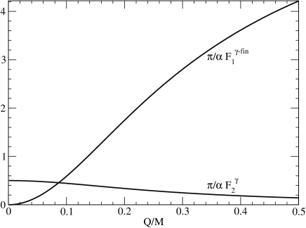
Figure 1: Photon-loop form factors $F_{1,2}^{\gamma}$ of the muon, where $F_{1}^{\gamma-{\rm fin}}$ refers to the infrared-finite part.

In this section, we discuss the photon-loop form factors of the muon and of the proton that appear in the expression for $H_{1}$, see Eq. (5). The photon-loop form factors of the muon are obtained from a standard QED calculation of the triangle diagram (and self-energy diagram which contributes through the muon wavefunction renormalization factor $Z_{2}$) and they explicitly read:

$$F_{1}^{\gamma} \!\!\!=\!\!\! {\alpha t\over 2\pi}\int_{4}^{\infty}\!dx{1\over x(xr-t)\sqrt{x^{2}-4x}}\bigg{\{}\big{[}2\xi_{\rm ir}+\ln r+\ln(x-4)\big{]}(x-2)+4-{3x\over 2}\bigg{\}}$$ (6)

$$\!\!\!=\!\!\! {\alpha\over\pi}\bigg{\{}(2\xi_{\rm ir}+\ln r)\bigg{(}{1\over 2}+{t-2r\over\sqrt{t^{2}-4rt}}\ln{\sqrt{4r-t}+\sqrt{-t}\over 2\sqrt{r}}\bigg{)}+{(2r-t)\over\sqrt{t^{2}-4rt}}\bigg{[}\ln^{2}{\sqrt{4r-t}+\sqrt{-t}\over 2\sqrt{r}}$$

$$+\bigg{(}{8r-3t\over 4r-2t}-\ln{4r-t\over r}\bigg{)}\ln{\sqrt{4r-t}+\sqrt{-t}\over 2\sqrt{r}}+{\rm Li}_{2}\bigg{(}{t-2r+\sqrt{t^{2}-4rt}\over 2r}\bigg{)}+{\pi^{2}\over 12}\bigg{]}-1\bigg{\}}\,,$$

$$F_{2}^{\gamma} = {2\alpha\over\pi}{r\over\sqrt{t^{2}-4rt}}\ln{\sqrt{4r-t}+\sqrt{-t}\over 2\sqrt{r}}\,.$$ (7)

The infrared divergence $\xi_{\rm ir}$ is defined as $\xi_{\rm ir}=\ln(M/m_{\gamma})$, with $m_{\gamma}$ an infinitesimal regulator photon mass. Moreover, Li${}_{2}(a)=a\int_{1}^{\infty}\!dx[x(x-a)]^{-1}\ln x$ denotes the conventional dilogarithmic function for $a<1$. One observes that the $F_{1,2}^{\gamma}$ are actually functions of the ratio $-t/r$ and the first version of $F_{1}^{\gamma}$ is a once-subtracted dispersion relation. Note that $F_{1}^{\gamma}(0)=0$ and $F_{2}^{\gamma}(0)=\alpha/2\pi=1.1614\!\cdot\!10^{-3}$ gives the leading correction to the muon anomalous magnetic moment. These form factors are shown (multiplied with $\pi/\alpha$) in Fig. 1, leaving out the regularization-dependent $\xi_{\rm ir}$ term for $F_{1}^{\gamma}$.

The photon-loop form factors of the proton are composed in a similar way of infrared-divergent and infrared-finite pieces:

$$G_{E,M}^{\gamma}={\alpha\over\pi}\xi_{\rm ir}\bigg{(}1+{2t-4\over\sqrt{t^{2}-4t}}\ln{\sqrt{4-t}+\sqrt{-t}\over 2}\bigg{)}G_{E,M}+G_{E,M}^{\gamma{\rm-fin}}+G_{E,M}^{\gamma\Delta}+G_{E,M}^{\gamma\Delta\Delta}\,,$$ (8)

where $G_{E,M}^{\gamma{\rm-fin}}$ denotes the infrared-finite part and $G_{E,M}^{\gamma\Delta}+G_{E,M}^{\gamma\Delta\Delta}$ arises from treating inelastic contributions through single and double $\Delta^{+}(1232)$ resonance excitation of the proton.

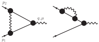
Figure 2: Photonic vertex and self-energy corrections with proton intermediate states.

The contributions to $G_{E,M}^{\gamma{\rm-fin}}$ from the triangle diagram in Fig. 2 can be calculated numerically as double-integrals ${\alpha\over\pi}\int_{0}^{\infty}\!dx\int_{-1}^{+1}\!dz\sqrt{1-z^{2}}\{[\dots]G_{E}(Q)+[\dots]G_{M}(Q)\}$ over cubic expressions in some given phenomenological form factors $G_{E,M}$. The proton form factors enter linearly in the external momentum transfer $Q$ and quadratically in the loop-momentum $xM$ inside the square brackets. The wave-function renormalization factor $Z_{2}$ from the self-energy diagram (see right part of Fig. 2) must also be taken into account in order to ensure that $G_{E}^{\gamma}(0)=0$. Using the representation of $Z_{2}$ in terms of an integral over the proton form factors as written in Eq. (5) of Ref. Kaiser:2016tbf , one gets $Z_{2}={\alpha\over\pi}\xi_{\rm ir}+Z_{2}^{\rm fin}$, where $Z_{2}^{\rm fin}$ depends weakly on the choice of proton form factors $G_{E,M}$.

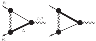
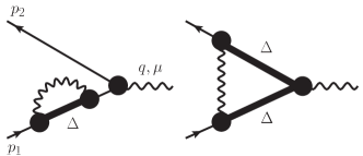
Figure 3: Photonic vertex and self-energy corrections with $\Delta^{+}(1232)$ intermediate states.

In this work we model inelastic contributions to the photon-loop form factors of the proton by single and double excitation of the $\Delta^{+}(1232)$ resonance, as shown in Fig. 3. As we will see later, this is appropriate here. More sophisticated approaches could also be entertained, see e.g. the review Arrington:2011dn , but we refrain from doing so here. The Lorentz-covariant description of the spin-$3/2$ $\Delta$-isobar requires a Rarita-Schwinger spinor $\Psi_{\alpha}$. We use a minimal gauge-invariant form of the $\Delta^{+}p\gamma$-vertex:

$${ie\kappa^{*}\over\sqrt{6}M}\big{(}g^{\mu\alpha}\gamma\!\cdot\!q-\gamma^{\mu}q^{\alpha}\big{)}\gamma_{5}\,G_{\Delta}(\sqrt{-q^{2}})\,,$$ (9)

in terms of the transition magnetic moment $\kappa^{*}\simeq 5.0$ and a phenomenological transition form factor

$$G_{\Delta}(Q)=\bigg{(}1+{Q^{2}\over\Lambda^{2}}\bigg{)}^{-2}\exp\bigg{(}-{Q^{2}\over 7\Lambda^{2}}\!\bigg{)}\,,$$ (10)

with dipole mass $\Lambda=843\,$MeV, as extracted from pion electroproduction in the $\Delta$-resonance region Albrecht:1971rv ; Galster:1972rh ; Burkert:1992yk . Here, $q$ denotes the space-like four-momentum carried by the virtual photon, so that $Q=\sqrt{-q^{2}}$. A commonly used form of the Rarita-Schwinger propagator (from index $\beta$ to index $\alpha$) reads:

$${i\over 3}\,{\gamma\!\cdot\!p+M_{\Delta}\over M_{\Delta}^{2}-p^{2}}\bigg{(}3g_{\alpha\beta}-\gamma_{\alpha}\gamma_{\beta}-{2p_{\alpha}p_{\beta}\over M_{\Delta}^{2}}+{p_{\alpha}\gamma_{\beta}-\gamma_{\alpha}p_{\beta}\over M_{\Delta}}\bigg{)}\,,$$ (11)

with $p$ the four-momentum of the propagating $\Delta$-isobar. The left two diagrams in Fig. 3 provide equal contributions to $G_{E,M}^{\gamma\Delta}$, respectively, and the condition $G_{E}^{\gamma\Delta}(0)=0$ follows immediately from the magnetic coupling vertex in Eq. (9). In order to evaluate the right diagram in Fig. 3, the $\Delta^{+}\Delta^{+}\gamma$-vertex is needed. It is naturally obtained by gauging the kinetic term of the free Rarita-Schwinger Lagrangian Benmerrouche:1989uc as:

$$ie\big{(}-\gamma^{\mu}g_{\alpha\beta}+\gamma_{\alpha}g_{\beta}^{\mu}+\gamma_{\beta}g_{\alpha}^{\mu}-\gamma_{\alpha}\gamma^{\mu}\gamma_{\beta}\big{)}\,$$ (12)

with $\beta$ the incoming and $\alpha$ the outgoing (Rarita-Schwinger) index. Further, we multiply this electric vertex with a dipole form factor times a (squared) exponential function as in Eq. (10). The third diagram in Fig. 3 contributes as $Z_{2}^{(\Delta)}G_{E,M}$, with the wavefunction renormalization factor $Z_{2}^{(\Delta)}$ written in Eq. (16) of Ref. Kaiser:2016tbf . It is worth to mention that only the combination of both right diagrams ensures the condition $G_{E}^{\gamma\Delta\Delta}(0)=0$ for the photon-loop induced electric form factor. The various contributions to the photon-loop proton form factors multiplied with $\pi/\alpha$ are shown in Fig. 4, for two choices of proton form factors, namely the well-known (simple) dipole form and the most recent parametrization based on dispersion theory, that describes essentially all data in the time-like and in the space-like regions Lin:2021xrc . We note that there are cancellations between the single- and the double-$\Delta$ contributions to both form factors, and that only the $\Delta$ contribution to the magnetic form factor is sizeable (on the scale of $\alpha/\pi=2.323\!\cdot\!10^{-3}$). Although the curve for $G_{E}^{\gamma-{\rm fin}}$ shown in Fig. 4 appears to drop linearly for small $Q$, the underlying analytical expression is manifestly even under $Q\to-Q$, and this is true for any form factor.

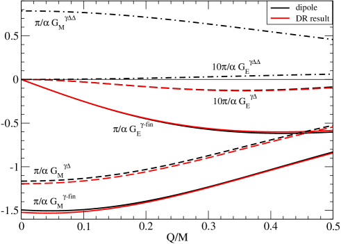
Figure 4: Various contributions to the electric and magnetic photon-loop form factors of the proton. The black lines represent results obtained by using the dipole parametrization and the red lines show the calculations based on the form factors from Ref. Lin:2021xrc .

IV Two-photon exchange box diagrams

We now consider the two-photon exchange correction incorporated in the $H_{2}$ term. For a point-like proton with $G_{E}=G_{M}=1$ the ratio $H_{2}/H_{0}$ can be inferred from the calculation in Sec. 3 of Ref. Kaiser:2010zz as:

$${H_{2}\over H_{0}}=-{2t\over A^{\prime}\otimes A^{\prime}}{\rm Re}({\rm III}^{\prime}\otimes A^{\prime}+{\rm IV}^{\prime}\otimes A^{\prime})\,,$$ (13)

where the change of sign is necessary, because there the case of equally charged leptons of different masses has been considered. The pertinent one-photon exchange term is $A^{\prime}\otimes A^{\prime}=2(s-1-r)^{2}+2st+t^{2}$ and ${\rm III}^{\prime}\otimes A^{\prime}$ is written in Eq. (31) of ref.Kaiser:2010zz , while ${\rm IV}^{\prime}\otimes A^{\prime}=-{\rm III}^{\prime}\otimes A^{\prime}|_{s\to u}$

For a structureless proton the ratio $H_{2}/H_{0}$ (setting $\xi_{\rm ir}=0$) at the AMBER kinematics ($E_{1}=100\,$GeV or $s\simeq 214$) is found to be rather small, starting from zero at $Q=0$ and increasing to about $0.016\%$ at $Q=M/2=469\,$MeV, see Fig. 5. This small value results from a strong cancellation between the planar and crossed $2\gamma$-exchange box graph, namely $7.743\%-7.727\%$. In the limit $Q\to 0$, where the cancelation becomes exact, the contributions from the planar and crossed box graph behave each as $\xi_{\rm ir}+\ln(Q/M)$ times an $(r,s)$-dependent factor of opposite sign. As also shown in Fig. 5, this cancellation is even more pronounced for the physical proton. For the nucleon intermediate state, we use the Feynman graph formalism of Ref. Lorenz:2014yda and the $\Delta$ intermediate state is evaluated using the dispersion relation approach of Refs. Blunden:2017nby ; Tomalak:2014sva . The ratio $H_{2}/H_{0}$ does not exceed the value $0.003\%$ for the low momentum transfers considered here.

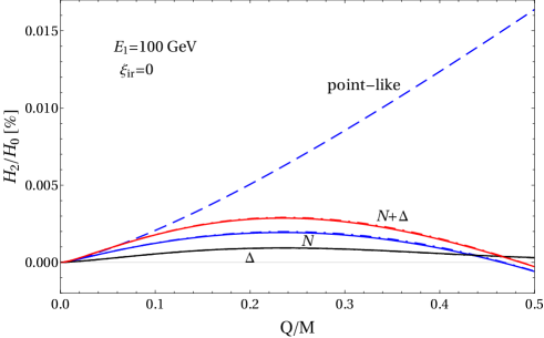
Figure 5: The ratio $H_{2}/H_{0}$ for a point-like proton (dashed line) and for the physical proton (lines labelled “$N+\Delta$”). The elastic contribution and the inelastic contribution (modelled by single $\Delta$-isobar excitation) are shown separately by the lines labelled “$N$” and “$\Delta$”. Solid lines refer to the use of the form factors from Ref. Lin:2021xrc and dot-dashed lines are based on dipole form factors.

V Soft photon radiation

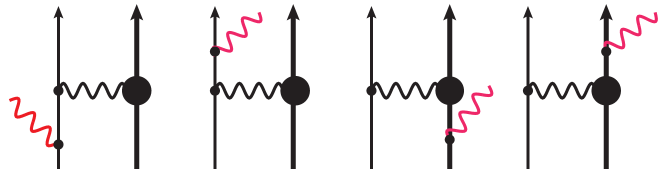
Figure 6: Diagrams representing the four amplitudes for soft photon radiation. Thin and solid lines denote muons and protons, respectively, while the wiggly lines denote photons. The corresponding (point-like and structureful) vertices are depicted by small and large filled circles.

Without the inclusion of the soft photon radiation the treatment of radiative corrections to $\mu^{-}p\to\mu^{-}p$ is incomplete or even meaningless. When working at higher order in the electromagnetic coupling $e$, the muon and proton can radiate a real photon with four-momentum $\ell$ and polarization vector $\epsilon$ in the initial or final state, as shown in Fig. 6. The corresponding soft amplitude reads:

$$e\bigg{(}{\epsilon\!\cdot\!k_{1}\over\ell\!\cdot\!k_{1}}-{\epsilon\!\cdot\!k_{2}\over\ell\!\cdot\!k_{2}}-{\epsilon\!\cdot\!p_{1}\over\ell\!\cdot\!p_{1}}+{\epsilon\!\cdot\!p_{2}\over\ell\!\cdot\!p_{2}}\bigg{)}\,,$$ (14)

where the soft momentum $\ell$ is neglected in the numerator, and the accompanying $\mu^{-}p\to\mu^{-}p$ process is kept in the limit $\ell=0$. Note that the signs in Eq. (14) indicate the charge of the radiating particle and whether this emission happens in the initial or the final state. The soft amplitude gets squared and summed over the two transversal polarizations by employing $\sum_{pol}\epsilon^{\mu}\epsilon^{\nu}=-g^{\mu\nu}$, which leads to:

$$4\pi\alpha\bigg{\{}-{m_{\mu}^{2}\over(\ell\!\cdot\!k_{1})^{2}}-{m_{\mu}^{2}\over(\ell\!\cdot\!k_{2})^{2}}-{M^{2}\over(\ell\!\cdot\!p_{1})^{2}}-{M^{2}\over(\ell\!\cdot\!p_{2})^{2}}$$

$$+{2k_{1}\!\cdot\!k_{2}\over\ell\!\cdot\!k_{1}\,\ell\!\cdot\!k_{2}}+{2p_{1}\!\cdot\!p_{2}\over\ell\!\cdot\!p_{1}\,\ell\!\cdot\!p_{2}}+{2k_{1}\!\cdot\!p_{1}\over\ell\!\cdot\!k_{1}\,\ell\!\cdot\!p_{1}}+{2k_{2}\!\cdot\!p_{2}\over\ell\!\cdot\!k_{2}\,\ell\!\cdot\!p_{2}}-{2k_{1}\!\cdot\!p_{2}\over\ell\!\cdot\!k_{1}\,\ell\!\cdot\!p_{2}}-{2k_{2}\!\cdot\!p_{1}\over\ell\!\cdot\!k_{2}\,\ell\!\cdot\!p_{1}}\bigg{\}}\,.$$ (15)

In any experiment with finite energy resolution, the emission of additional soft photons with $|\vec{\ell}\,|<\lambda$ is undetectable and thus gets subsumed in the cross section for the elastic scattering process. The integrals of the ten terms in Eq. (15) over a (small) momentum sphere $|\vec{\ell}\,|<\lambda$ are solved with the help of the following (infrared-regularized) master integral:

$$\int_{0}^{\lambda}\!\!d\ell{\ell^{2}\over 2\sqrt{m_{\gamma}^{2}+\ell^{2}}}\int_{-1}^{+1}\!\!dz{-1\over\big{(}E\sqrt{m_{\gamma}^{2}+\ell^{2}}-p\ell z\big{)}^{2}}={1\over E^{2}-p^{2}}\bigg{[}\ln{m_{\gamma}\over 2\lambda}+{E\over 2p}\ln{E+p\over E-p}\bigg{]}\,.$$ (16)

It applies directly to the first four terms in Eq. (15) with squares in the denominator, whereas for the six terms with products in the denominator one makes use of the Feynman parametrization: $(AB)^{-1}=\int_{0}^{1}\!dx[Ax+B(1\!-\!x)]^{-2}$. Putting all pieces together, the correction factor from soft photon radiation is given by the sum $\delta_{\rm soft}=\delta_{\rm soft}^{\rm(uni)}+\delta_{\rm soft}^{\rm(cm)}$, where the universal part reads:

$$\delta_{\rm soft}^{\rm(uni)} \!\!\!\!=\!\!\!\! {4\alpha\over\pi}\Big{(}\ln{M\over 2\lambda}-\xi_{\rm ir}\Big{)}\bigg{\{}1+{t-2r\over\sqrt{t^{2}-4rt}}\ln{\sqrt{4r-t}+\sqrt{-t}\over 2\sqrt{r}}+{t-2\over\sqrt{t^{2}-4t}}\ln{\sqrt{4-t}+\sqrt{-t}\over 2}$$

$$+{2(1+r-s)\over\sqrt{s-\rho_{+}}\sqrt{s-\rho_{-}}}\ln{\sqrt{s-\rho_{+}}+\sqrt{s-\rho_{-}}\over 2r^{1/4}}+{2(1+r-u)\over\sqrt{\rho_{+}-u}\sqrt{\rho_{-}-u}}\ln{\sqrt{\rho_{+}-u}+\sqrt{\rho_{-}-u}\over 2r^{1/4}}\bigg{\}},$$

with $\rho_{\pm}=1+r\pm 2\sqrt{r}$. It cancels exactly the infrared divergences proportional to $\xi_{\rm ir}$ from the virtual photon-loops and the remainder depends logarithmically on an infrared cut-off $\lambda$ for undetected soft photon radiation. Note that the last two terms cancel the infrared divergences from the two-photon exchange box diagrams. For these the antisymmetry under $s\leftrightarrow u$ is manifest by setting $\sqrt{u-\rho_{\pm}}=i\sqrt{\rho_{\pm}-u}$, $\sqrt{\rho_{\pm}-s}=i\sqrt{s-\rho_{\pm}}$ and taking eventually the real part of a logarithm. In the limit $r\to 0$ the sum of these two terms simplifies drastically to $\ln(1-u)-\ln(s-1)$. For $\mu^{+}p\to\mu^{+}p$ the last two terms in Eq. (LABEL:eq:softuni) change sign, keeping the role of $s$ and $u$.

The other part of $\delta_{\rm soft}$ is specific for assuming in the center-of-mass frame a small momentum sphere $|\vec{\ell}\,|<\lambda$ for undetected soft bremsstrahlung:

$$\delta_{\rm soft}^{\rm(cm)} \!\!\!\!=\!\!\!\! {\alpha\over\pi}\Bigg{\{}{2\over\sqrt{P}}\bigg{[}(s-1+r)\ln{s-1+r+\sqrt{P}\over 2\sqrt{sr}}+(s+1-r)\ln{s+1-r+\sqrt{P}\over 2\sqrt{s}}\,\bigg{]}$$ (18)

$$+\int_{0}^{1/2}\!\!\!dx\Bigg{[}{(t-2r)(s-1+r)\over[r-tx(1-x)]\sqrt{R_{t}}}\ln{s-1+r+\sqrt{R_{t}}\over s-1+r-\sqrt{R_{t}}}+{(t-2)(s+1-r)\over[1-tx(1-x)]\sqrt{R_{t}}}\ln{s+1-r+\sqrt{R_{t}}\over s+1-r-\sqrt{R_{t}}}\,\Bigg{]}$$

$$+\int_{0}^{1}\!\!dx\Bigg{[}{(1+r-s)[s+(1-r)(1-2x)]\over(1-2x)[sx(1-x)+(1-2x)(1-x-rx)]\sqrt{P}}\ln{s+(1-2x)(1-r+\sqrt{P})\over s+(1-2x)(1-r-\sqrt{P})}$$

$$\qquad\qquad+{(1+r-u)[s+(1-r)(1-2x)]\over[1+(r-1)x-ux(1-x)]\sqrt{R_{u}}}\ln{s+(1-r)(1-2x)+\sqrt{R_{u}}\over s+(1-r)(1-2x)-\sqrt{R_{u}}}\,\Bigg{]}\Bigg{\}}\,,$$

introducing the auxiliary polynomials $R_{t}=P+4stx(1-x)$ and $R_{u}=P+4x(1-x)[su-(1-r)^{2}]$, with $P=s^{2}-2s(1+r)+(1-r)^{2}$. Although possible, we refrain from solving the Feynman-parameter integrals in Eq. (18) which lead to overly complicated expressions involving squared logarithms and dilogarithms (see e.g. Eqs.(4.10)-(4.12) in Ref. Maximon:2000hm ). For $\mu^{+}p\to\mu^{+}p$ the last term $\int_{0}^{1}\!dx\dots$ changes sign, keeping the role of $s$ and $u$.

VI Results and discussion

We can now put the pieces together and discuss the radiative corrections to muon-proton scattering. First, it is interesting to see how much the radiative corrections to $\mu^{-}p\to\mu^{-}p$ scattering (at a beam energy of $E_{1}=100\,$GeV) are affected by the underlying proton structure. For that purpose we make comparisons with a structureless proton, corresponding to $G_{E,M}=1$. Returning to Eq. (2), one recognizes that the radiative corrections (i.e. changes of cross section ratios) from vacuum polarization and soft photon bremstrahlung are the same for a structureful and structureless proton. Concerning the ratio $H_{1}/H_{0}$, one finds that this feature still holds for the muonic part written in the first line in Eq. (5). To high accuracy this ratio is equal to $2F_{1}^{\gamma}$, because the other muon form factor $F_{2}^{\gamma}$ is suppressed by a factor of the muon mass squared, and it enters with a further suppression factor $t$. Interestingly, the situation is different for the vertex corrections at the proton, described by $G_{E,M}^{\gamma}$ in the second line of Eq. (5). As shown in the left panel of Fig. 7, for a structureless proton and one finds that this part of the ratio $H_{1}/H_{0}$ grows from zero to $1.33\cdot 10^{-4}$ in the momentum transfer region $0<Q<M/2$. If these vertex corrections, specified by $G_{E,M}^{\gamma-{\rm fin}}$, are evaluated with phenomenological form factors, the corresponding radiative correction $H_{1}/H_{0}$ is negative and reaches more significant values of about $-0.4\%$. Further effects from inelastic contributions (modelled here by $\Delta^{+}(1232)$-resonance excitations) turn out to be of magnitude $10^{-4}$ and are thus not relevant in view of the experimental accuracy, see the right panel of Fig. 7.

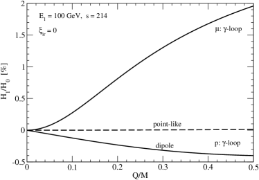
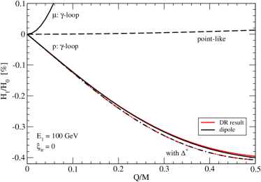
Figure 7: Ratio $H_{1}/H_{0}$ due to electromagnetic vertex corrections separated into parts from the muon and the proton. Left panel: Corrections from the photon-loop around the muon, the point-like proton and the composite proton using dipole form factors. Right panel: Zoom in on the proton contribution using dipole form factors as well as the most recent form factors from dispersion theory Lin:2021xrc . The solid and dot-dashed lines refer to the elastic and elastic plus inelastic contribution.

In Fig. 8 we show the radiative corrections from all discussed sources (of order $\alpha/\pi$) for the planned AMBER experiment with a muon beam energy of $E_{1}=100\,$GeV and an assumed infrared cutoff of $\lambda=20\,$MeV, corresponding to an energy resolution that limits the detection of photons with an energy below $20\,$MeV. We set $\xi_{\rm ir}=0$ in order to have all individual contributions independent of the regulator mass $m_{\gamma}$. At small momentum transfers $Q/M\lesssim 0.06$, vacuum polarization is the most dominant effect, because it is driven by the electron mass scale. After that, the soft-photon radiation takes over, with a sizeable contribution (of $2\%$) from the photon-loop form factor $2F_{1}^{\gamma-{\rm fin}}$, involving the muon mass scale, at the upper end of the momentum transfers considered here. The negative photon-loop form factor contribution from the proton stays below $0.4\%$ in magnitude, and the two-photon exchange correction of maximal size $0.3\cdot 10^{-4}$ can essentially be neglected.

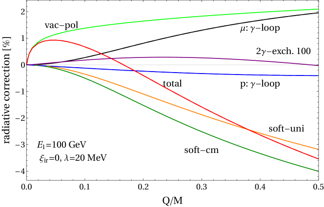
Figure 8: Radiative corrections for the AMBER kinematics with $E_{1}=100\,$GeV. The individual radiative corrections from vacuum polarization, the virtual photon-loops and soft bremsstrahlung are shown together with their sum, see the solid line labelled “total”.

As a variation we show in Fig. 9 the radiative corrections for a smaller muon beam energy of $E_{1}=50\,$GeV (as it is also planned by AMBER) and the same infrared cutoff of $\lambda=20\,$MeV. In comparison to the case with $E_{1}=100\,$GeV, one observes an increase of the two-photon exchange correction and some slight changes in the soft photon components, but the overall pattern is nearly the same.

VII Summary and outlook

In this work we have systematically calculated the radiative corrections of order $\alpha/\pi$ to elastic muon-proton scattering. These corrections consist of vacuum polarization, soft photon radiation, photon-loop form factors of the muon and of the proton, and two-photon exchange corrections. The first three components turn out to be universal in the sense that the structure of the proton (as encoded in the electric and magnetic form factors $G_{E,M}$) drops out in the respective ratios to the Born cross section. The photon-loop induced vertex corrections at the proton give rise to additional form factors $G_{E,M}^{\gamma}\sim\alpha/\pi$, whose infrared finite pieces can be calculated with sufficient accuracy. The elastic contribution to $G_{E,M}^{\gamma}$ from the proton intermediate state is almost independent of the input form factors into the pertinent triangle diagram, while inelastic contributions (modelled here by excitation of the low-lying $\Delta(1232)$-resonance) play numerically no role for the relevant ratio $H_{1}/H_{0}$. The same is even more true for the two-photon exchange, whose relative effect measured by the ratio $H_{2}/H_{0}$ stays well below $10^{-4}$ in the small momentum transfer region $Q<400\,$MeV. Therefore, the aspects of proton structure that enter the virtual radiative corrections do not limit the precision of extracting the form factors $G_{E,M}$, and finally the proton radius $r_{p}$, accurately from elastic muon-proton scattering

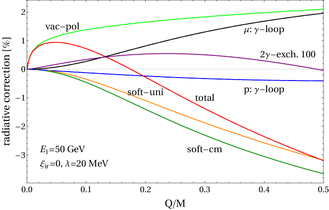
Figure 9: Radiative corrections for the AMBER kinematics with $E_{1}=50\,$GeV. Same notation as in Fig. 8.

With the complete radiative corrections of the size of a few percent and aiming for permille accuracy, a prominent role is played by the soft photon radiation. The treatment of undetected soft photon bremsstahlung in this work in terms of a small momentum sphere $|\vec{\ell}\,|<\lambda$ in the center-of-mass frame corresponds to an idealized experiment. In a real experiment this region in phase space has a more complicated structure with smooth edges due to varying detector acceptances and other effects. By computing the fivefold differential cross section $d^{5}\sigma/(d\Omega_{\mu}d\Omega_{\gamma}d\omega_{\gamma})$ for the process $\mu^{\mp}p\to\mu^{\mp}p\gamma$ at tree-level, and integrating it over the experimentally “blind regions” (of course, now with exclusion of the small momentum sphere $|\vec{\ell}\,|<\lambda$) the treatment of undetected soft and hard photon bremsstahlung can be tailored to the specific experimental conditions. At the same time this fivefold differential cross section can be used for experimental verification of its spectral and angular distributions in regions where additional photons are detectable. Work along these lines in collaboration with members of the AMBER collaboration is in progress.

References

- (1) S. Bifani, S. Descotes-Genon, A. Romero Vidal and M. H. Schune, J. Phys. G 46, no.2, 023001 (2019) [arXiv:1809.06229 [hep-ex]].
- (2) E. J. Downie [MUSE], EPJ Web Conf. 73, 07005 (2014).
- (3) B. Adams et al. [arXiv:1808.00848 [hep-ex]].
- (4) R. Pohl, R. Gilman, G. A. Miller and K. Pachucki, Ann. Rev. Nucl. Part. Sci. 63, 175-204 (2013) [arXiv:1301.0905 [physics.atom-ph]].
- (5) Y. H. Lin, H. W. Hammer and U.-G. Meißner, Phys. Rev. Lett. 128, no.5, 052002 (2022) [arXiv:2109.12961 [hep-ph]].
- (6) Y. H. Lin, H. W. Hammer and U.-G. Meißner, Eur. Phys. J. A 57, no.8, 255 (2021) [arXiv:2106.06357 [hep-ph]].
- (7) R. Pohl et al., Nature 466, 213-216 (2010).
- (8) H. Fleurbaey et al., Phys. Rev. Lett. 120, 183001 (2018) [arXiv:1801.08816 [physics.atom-ph]].
- (9) N. Bezginov, T. Valdez, M. Horbatsch, A. Marsman, A. C. Vutha and E. A. Hessels, Science 365, 1007 (2019).
- (10) A. Grinin et al., Science 370, 1061 (2020).
- (11) A. D. Brandt, S. F. Cooper, C. Rasor, Z. Burkley, D. C. Yost and A. Matveev, Phys. Rev. Lett. 128, no.2, 023001 (2022) [arXiv:2111.08554 [physics.atom-ph]].
- (12) W. Xiong et al., Nature 575, 147 (2019).
- (13) A. Gasparian et al. [PRad], [arXiv:2009.10510 [nucl-ex]].
- (14) A. Denig, J. Univ. Sci. Tech. China 46, no.7, 608-616 (2016).
- (15) N. Kaiser, J. Phys. G 37, 115005 (2010).
- (16) N. Kaiser, J. Phys. G 44, no.5, 055003 (2017) [arXiv:1610.05132 [nucl-th]].
- (17) O. Tomalak and M. Vanderhaeghen, Eur. Phys. J. C 76, no.3, 125 (2016) [arXiv:1512.09113 [hep-ph]].
- (18) O. Tomalak and M. Vanderhaeghen, Eur. Phys. J. C 78, no.6, 514 (2018) [arXiv:1803.05349 [hep-ph]].
- (19) C. Peset, A. Pineda and O. Tomalak, Prog. Part. Nucl. Phys. 121, 103901 (2021) [arXiv:2106.00695 [hep-ph]].
- (20) S. Actis et al. [Working Group on Radiative Corrections and Monte Carlo Generators for Low Energies], Eur. Phys. J. C 66, 585-686 (2010) [arXiv:0912.0749 [hep-ph]].
- (21) J. Arrington, P. G. Blunden and W. Melnitchouk, Prog. Part. Nucl. Phys. 66, 782-833 (2011) [arXiv:1105.0951 [nucl-th]].
- (22) W. Albrecht et al. Nucl. Phys. B 27, 615-620 (1971) [erratum: Nucl. Phys. B 30, 642-642 (1971)].
- (23) S. Galster, G. Hartwig, H. Klein, J. Moritz, K. H. Schmidt, W. Schmidt-Parzefall, D. Wegener and J. Bleckwenn, Phys. Rev. D 5, 519-527 (1972).
- (24) V. Burkert and Z. J. Li, Phys. Rev. D 47, 46-50 (1993).
- (25) M. Benmerrouche, R. M. Davidson and N. C. Mukhopadhyay, Phys. Rev. C 39, 2339-2348 (1989).
- (26) I. T. Lorenz, U.-G. Meißner, H. W. Hammer and Y. B. Dong, Phys. Rev. D 91, no.1, 014023 (2015) [arXiv:1411.1704 [hep-ph]].
- (27) P. G. Blunden and W. Melnitchouk, Phys. Rev. C 95 (2017) no.6, 065209 [arXiv:1703.06181 [nucl-th]].
- (28) O. Tomalak and M. Vanderhaeghen, Eur. Phys. J. A 51, no.2, 24 (2015) [arXiv:1408.5330 [hep-ph]].
- (29) L. C. Maximon and J. A. Tjon, Phys. Rev. C 62, 054320 (2000) [arXiv:nucl-th/0002058 [nucl-th]].