Exploring interpolating momentum schemes

Abstract

We compute the renormalisation factors of the quark mass and wave function using IMOM (Interpolating MOMenta) schemes. The framework is the Rome-Southampton non-renormalisation method, but the momentum transfer in the quark bilinears is not restricted to zero or to the symmetric point. We study the scale dependence, infrared contamination and lattice artefacts for different values of this momentum transfer and for two different kinds of projectors. For the numerical simulations, we use data generated by the RBC-UKQCD collaborations, with $N_{f}=2+1$ flavours of Domain-Wall fermions, and inverse lattice spacing of $1.79$ and $2.38$ GeV.

1 Kinematics

In the framework of the Rome-Southampton method [1], one imposes a set of renormalisation conditions on composite operator Green’s functions computed non-perturbatively on the lattice. We consider here a generic flavour non-singlet quark bilinear $O_{\Gamma}=\bar{\psi}_{i}\Gamma\psi_{j}$, where $i\neq j$ and $\Gamma$ is a Dirac matrix. We suppress the flavour indices $i$ and $j$ for simplicity. Traditionally the momentum transfer is chosen is to be either zero or such that $p_{1}^{2}-p_{2}^{2}=(p_{1}-p_{2})^{2}$, where $p_{1}$ and $p_{2}$ are the incoming and outgoing momenta, respectively (see Fig. 1).

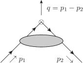
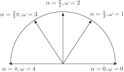
Figure 1: Left: a quark bilinear with incoming momentum $p_{1}$, outgoing momentum $p_{2}$ and momentum transfer $q=p_{1}-p_{2}$. Right: relationship between $\omega$ and the angle $\alpha$ between the incoming and outgoing momenta.

The former is known to lead to exceptional kinematics and therefore potentially large unwanted infrared contributions; the latter is referred to as the symmetric point and defines a so-called RI/SMOM scheme [2, 3]. The main purpose of the RI/SMOM kinematics is to suppress the unwanted low-energy contributions. Here we want to generalise this choice of kinematics. As usual, the renormalisation scale is called $\mu$, but we define an additional parameter $\omega$ such that

$$(p_{1}-p_{2})^{2} = \omega\mu^{2}\;,$$ (1.1)

$$\mu^{2} = p_{1}^{2}=p_{2}^{2}\;.$$ (1.2)

It follows that $\omega=0$ corresponds to zero-momentum transfer and $\omega=1$ corresponds to the RI/SMOM kinematics. Although it makes sense to fix $\omega$ to either of these values in order to be left with only one scale in the game, in general the parameter $\omega$ can take any value between $0$ and $4$. One can define an angle $\alpha$ between $p_{1}$ and $p_{2}$ and we find that $\omega=2(1-\cos\alpha)$, as illustrated in Fig. 1. It is clear that the extreme values of $\omega$ where $p_{1}$ and $p_{2}$ are parallel or anti-parallel can lead to collinear singularities. Letting $\omega$ vary as a free parameter defines the RI/IMOM schemes (we will now drop the “RI” to ease the notations). The interested reader can find more details in [4].

2 Definitions

2.1 Z-factors

We study $Z_{m}$ and $Z_{q}$, the renormalisation factors of the quark mass and wave function, respectively. The are defined in the chiral limit ($m$ represents the quark mass) through

$$Z_{q}^{(X)}(\mu,\omega) = Z_{V}\lim_{m\to 0}\left[\Lambda_{V}^{(X)}\right]_{\text{IMOM}}\;,$$ (2.3)

$$Z_{m}^{(X)}(\mu,\omega) = \frac{1}{Z_{V}}\lim_{m\to 0}\left[\frac{\Lambda_{S}}{\Lambda_{V}^{(X)}}\right]_{\text{IMOM}}\;.$$ (2.4)

On the right-hand-side of Eqs. (2.3) and (2.4), $\Lambda_{S,P}$ represent the amputated and projected vertex functions computed on Landau-gauge fixed configurations, at finite quark mass $m=Z_{m}m_{bare}$ (we take all quark masses to be same for simplicity). The values of $Z_{V}$ are known from previous work [5]. The choice of projector is denoted by $X\in(\gamma_{\mu},q\!\!\!/)$, more explicitly:

$$\Lambda_{S} = \frac{1}{12}\text{Tr}[\Pi_{S}]\;,$$ (2.5)

$$\Lambda_{V}^{(\gamma_{\mu})} = \frac{1}{48}\text{Tr}[\gamma_{\mu}\Pi_{V^{\mu}}]\;,$$ (2.6)

$$\Lambda_{V}^{(\not{q})} = \frac{q^{\mu}}{12q^{2}}\text{Tr}[\not{q}\Pi_{V^{\mu}}\,]\;,$$ (2.7)

where $\Pi_{\Gamma},\Gamma=S,{V^{\mu}}$ represents the amputated vertex function:

$$\Pi_{\Gamma}=\langle G^{-1}(-p_{2})\rangle V_{\Gamma}(p_{2},p_{1})\langle G^{-1}(p_{1})\rangle\;,$$ (2.8)

and

$$V_{\Gamma}(p_{2},p_{1}) = \langle\psi(p_{2})O_{\Gamma}\bar{\psi}(p_{1})\rangle\;,$$ (2.9)

$$= \sum_{x}\langle G_{x}(-p_{2})\Gamma G_{x}(p_{1})\rangle\;,$$ (2.10)

$$G(p) = \sum_{x}G_{x}(p)\;.$$ (2.11)

Finally, within our conventions, $G_{x}(p)$ represents an incoming quark propagator with momentum $p$, where the Fourier transform is computed at space-time point $x$, explicitly:

$$G_{x}(p)=\sum_{y}D^{-1}(x,y)e^{ip.(y-x)}.$$ (2.12)

In order to assess some systematic errors, we also implement the vertex function for $\Lambda_{A}$ and $\Lambda_{P}$. They are defined exactly in the same way, with $V\longrightarrow A$ and $S\longrightarrow P$ in the previous equations

2.2 Running

We compute the non-perturbative scale evolution of $Z_{y},y\in(m,q)$, we define $\Sigma_{m}$ as:

$$\Sigma^{(X)}_{y}(a,\mu,\mu_{0},\omega,\omega_{0})=\lim_{m\rightarrow 0}\frac{Z^{(X)}_{y}(a,\mu,\omega)}{Z^{(X)}_{y}(a,\mu_{0},\omega_{0})}\;,$$ (2.13)

where as above $X$ can be either $\gamma_{\mu}$ or $\not{q}$. We take the continuum limit :

$$\sigma^{(X)}_{y}(\mu,\mu_{0},\omega,\omega_{0})=\lim_{a^{2}\rightarrow 0}\Sigma^{(X)}_{y}(a,\mu,\mu_{0},\omega,\omega_{0})\;.$$ (2.14)

We also compute this running in perturbation theory at Next-to-Next-to-Leading Order (NNLO). We note that for $Z_{m}$, the corresponding anomalous dimensions have been recently computed in [6] and [7] at N³LO in the case $\omega=1$. In $\overline{\text{MS}}$, they can be found in [8], together with the one of the quark wave function for the $q\!\!\!/$-projector.

3 Results

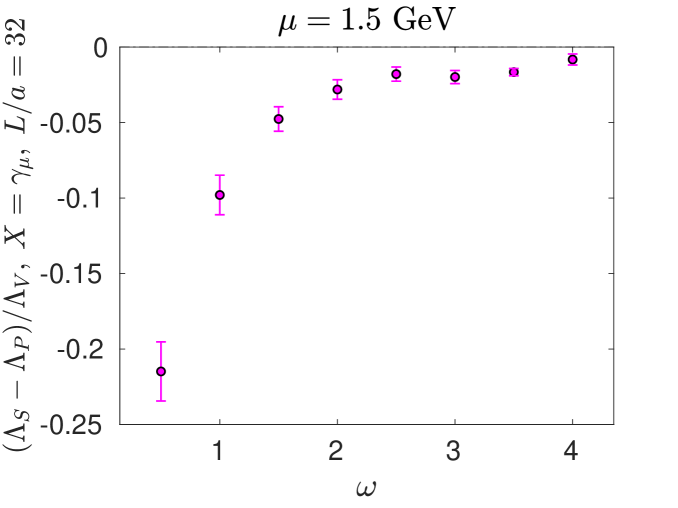
Figure 2: As a measure of chiral symmetry breaking effects we show $(\Lambda_{S}-\Lambda_{P})/\Lambda_{V}$ for the ${\gamma_{\mu}}$-projector, as a function of $\omega$, for a fixed value of $\mu$. The unwanted low energy contributions decrease quickly as $\omega$ increases.

As it is often the case for a NPR study, the choice of the lattice discretisation is of crucial importance. The good chiral-flavour properties of the Domain-Wall fermions are essential to disentangle physical infrared contributions from artefacts due to the choice of fermionic action. In absence of chiral symmetry breaking, we should find $\Lambda_{S}=\Lambda_{P}$. In Fig. 2, we show $(\Lambda_{S}-\Lambda_{P})/\Lambda_{V}$ as a function of $\omega$, for $\mu=1.5$ GeV (we divide by $\Lambda_{V}$ to cancel the quark wave function renormalisation factor). We find that this quantity is much smaller for $\omega\geq 2$ than for $\omega=1$: $\sim 0.03$ vs. $\sim 0.10$ . This could be important for four-quark operators such as $(S-P)\times(S-P)$ and $(S-P)\times(S+P)$ which can also mix due to chiral symmetry breaking effects.

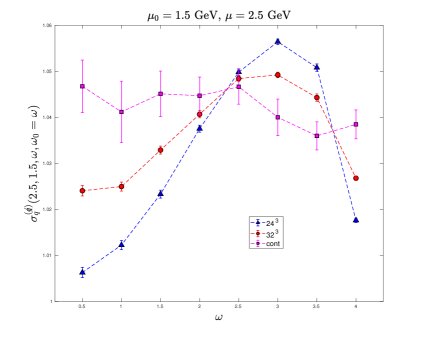
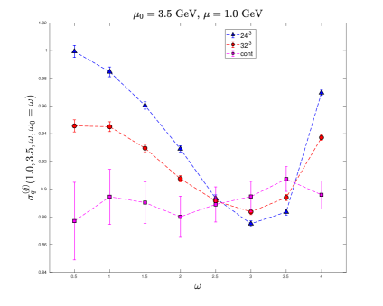
Figure 3: Example of continuum extrapolations for $\sigma_{q}^{(q\!\!\!/)}(\mu,\mu_{0},\omega,\omega_{0})$.

In Fig.3 we show the non-perturbative scale evolution for $Z_{q}^{(q\!\!\!/)}$ at finite lattice spacing and in the continuum, for different values of $\omega=\omega_{0}$. We expect this quantity to be $\omega$-independent due to the vector Ward-Takahashi identity. Although after continuum extrapolation this quantity is indeed $\omega$-independent (to a good approximation), this is clearly not the case at finite lattice spacing. Using this quantity as a measure of the discretisation effects, Fig.3 suggests that the region $\omega\sim 2.0-2.5$ is less affected by lattice artefacts (for this quantity).

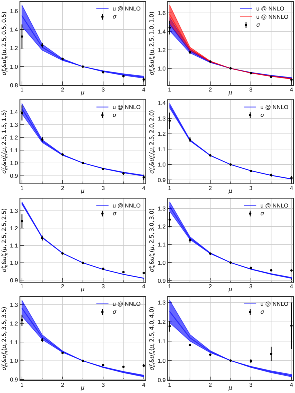
Figure 4: Comparison of the non-perturbative and perturbative running for $Z_{m}^{(\gamma_{\mu})}$. Note that for $\omega=1$ the perturbative running is known at N³LO.

We show the running of the quark mass in Fig. 4 for the $\gamma_{\mu}$-scheme: both the non-perturbative scale evolution $\sigma^{(\gamma_{\mu})}_{m}(\mu,\mu_{0},\omega,\omega_{0})$ and the perturbative prediction $u^{(\gamma_{\mu})}_{m}(\mu,\mu_{0},\omega,\omega_{0})$. We fix $\omega=\omega_{0}=0.5,1.0,1.5,\ldots,4.0$ and let $\mu$ vary between 1 and 4 GeV. We find a good agreement for intermediate values of $\mu$ and $\omega$, where both perturbation theory and lattice artefacts are expected to be under control. There is also a good agreement for small values of $\mu$ (within our statistical and systematic uncertainties) where we would have expected non-perturbative effects to be more visible. We also find that out of the two projectors, perturbation theory and lattice results agree best in the $\gamma_{\mu}$-scheme. On the other hand, the lattice artefacts for large values of $\mu$ and $\omega$ become relevant for $q^{2}\gtrsim 25\mathrm{GeV}^{2}$. This becomes particularly visible for large values of $\omega=4$, where perturbation theory also becomes less reliable.

The only significant (relative) discrepancy we found is for $Z_{q}^{(q\!\!\!/)}$, the quark wave function in the $q\!\!\!/$-scheme. However, this quantity should be $\omega$-independent (up to lattice artefacts) and has no $\mu$-dependence at leading order (in the Landau gauge). We show our results in Tables 1 and 2. In this case the perturbative prediction is known at N³LO. As we can see from these tables, the series converges very poorly in the sense that the relative difference decreases very slowly as we increase the order of the expansion. The difference between the non-perturbative result and the N³LO prediction, namely $\sim 1.0195-1.0113\sim 0.0082$, could then be explained by higher corrections. On the other hand, for $X=\gamma_{\mu}$, we find a much better convergence of the perturbative expansion and a good agreement between the perturbative and non-perturbative running after conversion to $\overline{\text{MS}}$.

Scheme	LO	NLO	NNLO	NNNLO	NP
$\overline{\text{MS}}$	1.0	1.0048	1.0062	1.0064
$\overline{\text{MS}}\leftarrow\gamma_{\mu}$	1.0	1.0069	1.0078	N.A.
$\overline{\text{MS}}\leftarrow q\!\!\!/$	1.0	1.0195	1.0175	1.0146
$\gamma_{\mu}$	1.0	1.0017	1.0020	N.A	1.0037(20)
$q\!\!\!/$	1.0	1.0048	1.0081	1.0113	1.0195(25)

Table 1: Running between 2 and 2.5 GeV for the quark wave function in $\overline{\text{MS}}$ and in the SMOM schemes $\gamma_{\mu}$($\omega=1$) and $q\!\!\!/$. In this case the running is known at NNNLO.

Scheme	NLO-LO	NNLO-NLO	NNNLO-NNLO
$\overline{\text{MS}}$	0.0048	0.0013	0.0003
$\gamma_{\mu}$	0.0017	0.0003
$q\!\!\!/$	0.0048	0.0033	0.0032

Table 2: Study of the convergence of the perturbative series for running of the quark wave function between 2 and 2.5 GeV in $\overline{\text{MS}}$, SMOM-$\gamma_{\mu}$ and $q\!\!\!/$.

4 Conclusions and outlook

We have implemented several IMOM schemes defined via two different projectors and determined the renormalisation factors and non-perturbative scale evolution functions of the quark mass and wave function. We find that the non-pertubative and perturbative results agree very well as long as we stay from the corner of the $\omega,\mu$ plane, with one exception, namely $Z_{q}^{(q\!\!\!/)}$. There, we argued that the reason for this relatively bad agreement is the poor convergence of the perturbative expansion. We have shown some cases where $\omega\sim 2.0-2.5$ lead to substantially reduced infrared contamination and better control over the discretisation effects, compared to standard SMOM kinematics.

We used two lattice spacings in this proof of concept study, clearly adding a finer lattice could potentially allow us to probe the Rome-Southampton window even further. It will also be interesting to extend this study to the case of four-quark operators where the infrared contaminations due to chiral symmetry breaking are significantly more sizeable. The hope is that increasing the value of $\omega$ will reduce these contaminations (compared to $\omega=1$) as it does for the bilinears.

5 Acknowledgements

This work was supported by the Consolidated Grant ST/T000988/1 and the work of JAG by a DFG Mercator Fellowship. The quark propagators were computed on the DiRAC Blue Gene Q Shared Petaflop system at the University of Edinburgh, operated by the Edinburgh Parallel Computing Centre on behalf of the STFC DiRAC HPC Facility (www.dirac.ac.uk). This equipment was funded by BIS National E-infrastructure capital grant ST/K000411/1, STFC capital grant ST/H008845/1, and STFC DiRAC Operations grants ST/K005804/1 and ST/K005790/1. DiRAC is part of the National E-Infrastructure.

We warmly thank our colleagues of the RBC and UKQCD collaborations. We are particularly indebted to Peter Boyle, Andreas Jüttner, J Tobias Tsang for many interesting discussions. We also thank Peter Boyle for his help with the UKQCD hadron software. We wish to thank Holger Perlt for his early contribution in this area. N.G. thanks his collaborators from the California Lattice (CalLat) collaboration and in particular those working on NPR: David Brantley, Henry Monge-Camacho, Amy Nicholson and André Walker-Loud.

- [1] G. Martinelli, C. Pittori, C. T. Sachrajda, M. Testa, and A. Vladikas, “A General method for nonperturbative renormalization of lattice operators,” Nucl. Phys. B445 (1995) 81–108, arXiv:hep-lat/9411010 [hep-lat].
- [2] Y. Aoki et al., “Non-perturbative renormalization of quark bilinear operators and B(K) using domain wall fermions,” Phys. Rev. D 78 (2008) 054510, arXiv:0712.1061 [hep-lat].
- [3] C. Sturm, Y. Aoki, N. H. Christ, T. Izubuchi, C. T. C. Sachrajda, and A. Soni, “Renormalization of quark bilinear operators in a momentum-subtraction scheme with a nonexceptional subtraction point,” Phys. Rev. D80 (2009) 014501, arXiv:0901.2599 [hep-ph].
- [4] N. Garron, C. Cahill, M. Gorbahn, J. Gracey, and P. Rakow, “Non-perturbative renormalisation with interpolating momentum schemes,” arXiv:2112.11140 [hep-lat].
- [5] RBC, UKQCD Collaboration, Y. Aoki et al., “Continuum Limit Physics from 2+1 Flavor Domain Wall QCD,” Phys. Rev. D 83 (2011) 074508, arXiv:1011.0892 [hep-lat].
- [6] A. Bednyakov and A. Pikelner, “Quark masses: N3LO bridge from to scheme,” Phys. Rev. D 101 (May, 2020) 091501. https://link.aps.org/doi/10.1103/PhysRevD.101.091501.
- [7] B. A. Kniehl and O. L. Veretin, “Bilinear quark operators in the RI/SMOM scheme at three loops,” Physics Letters B 804 (2020) 135398. http://www.sciencedirect.com/science/article/pii/S0370269320302021.
- [8] K. Chetyrkin and A. Rétey, “Renormalization and running of quark mass and field in the regularization invariant and MS-bar schemes at three loops and four loops,” Nucl. Phys. B 583 (2000) 3–34, arXiv:hep-ph/9910332.