Temporal Logic Guided Motion Primitives for Complex Manipulation Tasks with User Preferences

Abstract

Dynamic movement primitives (DMPs) are a flexible trajectory learning scheme widely used in motion generation of robotic systems. However, existing DMP-based methods mainly focus on simple go-to-goal tasks. Motivated to handle tasks beyond point-to-point motion planning, this work presents temporal logic guided optimization of motion primitives, namely $\textrm{P{I}}^{\textrm{BB-TL}}$ algorithm, for complex manipulation tasks with user preferences. In particular, weighted truncated linear temporal logic (wTLTL) is incorporated in the $\textrm{P{I}}^{\textrm{BB-TL}}$ algorithm, which not only enables the encoding of complex tasks that involve a sequence of logically organized action plans with user preferences, but also provides a convenient and efficient means to design the cost function. The black-box optimization is then adapted to identify optimal shape parameters of DMPs to enable motion planning of robotic systems. The effectiveness of the $\textrm{P{I}}^{\textrm{BB-TL}}$ algorithm is demonstrated via simulation and experiment.

I INTRODUCTION

By operating beyond structured environments, robots are moving towards applications in complex and unstructured environments, including offices, hospitals, homes [1]. These applications often require robots to be able to autonomously learn, plan, and execute a variety of challenging manipulations. As an enabling technique, dynamic movement primitives (DMPs) have emerged as a flexible trajectory learning scheme [2, 3, 4] for manipulators and mobile robots, such as biped walking of humanoid robots [5], collaborative manipulation of clothes [6], bimanual tasks [7]. While it is powerful, conventional DMPs are mainly limited to simple go-to-goal tasks. Another challenge that receives little attention in prior DMP-based approaches is the problem of capturing user preferences during motion and trajectory generation. Therefore, this work is particularly motivated to improve DMP-based motion generation skills for robotic systems to perform manipulations that consist of a sequence of logically organized actions with user preferences.

Related works: DMPs are encoded as a combination of simple linear dynamical systems with nonlinear components to acquire smooth movements of arbitrary shape. One common objective is to obtain the optimal parameters of nonlinear components. As discussed in [8], the trajectory generated by DMPs has good scaling properties with respect to the initial/end positions, the parameter linearity, the rescaling robustness, and the continuity. For these reasons, DMPs have been widely used with policy search reinforcement learning to identify a best policy (i.e., the optimal DMP parameters). Example policy search methods include gradient based approaches [9], expectation maximization based approaches [10], and information-theoretic approaches [11]. The policy improvement with path integrals algorithm $\textrm{P{I}}^{\textrm{2}}$ was derived from the first principles of stochastic optimal control [12, 13]. Different with gradient-based reinforcement learning algorithms, the $\textrm{P{I}}^{\textrm{2}}$ algorithm avoids the curse of dimensionality and gradient estimation by using parameterized policies with probability-weighted averaging. However, the motion primitive parameters for each dimension must be optimized individually when using $\textrm{P{I}}^{\textrm{2}}$ algorithm, which increases the computational complexity and reduces the parameter convergence rate. A stochastic optimization algorithm, namely Policy Improvement with Black-Box Optimization $\textrm{P{I}}^{\textrm{BB}}$, was then developed in [14]. As a special case of $\textrm{P{I}}^{\textrm{2}}$, $\textrm{P{I}}^{\textrm{BB}}$ uses the same method for exploration and parameter updating, but differs in using black-box optimization rather than reinforcement learning for policy improvement. Since $\textrm{P{I}}^{\textrm{BB}}$ is based on covariance matrix adaptation through weighted averaging, it can optimize the parameters of motion primitives with multiple dimensions simultaneously for improved efficiency and convergence rate. Other representative works that exploit DMP for motion generation include [12, 7, 15]. However, limited to the form of the expect cost function, neither $\textrm{P{I}}^{\textrm{BB}}$ nor $\textrm{P{I}}^{\textrm{2}}$ can handle parameter optimization of motion primitives for manipulation tasks with complex logic and temporal constraints.

Temporal logic, as a formal language, is capable of describing a wide range of complex tasks in a succinct and human-interpretable form, and thus has been increasingly used in the motion planning of robotic systems [16, 17, 18, 19, 20, 21]. Signal temporal logic (STL) is defined over continuous signals and its quantitative semantics, known as robustness, can measure the degree of satisfaction or violation of the desired task specification [22]. To maximize the robustness of STL, the synthesis problem is often cast as optimization problems and then solved using heuristics, mixed-integer programming or gradient methods [23, 24, 25, 26, 27]. However, STL formulas specify subtasks with explicit time bounds, while many manipulation tasks only require the subtasks to be performed in a desired sequence (e.g., open the fridge door, take the milk out, and close the fridge door). Manually assigning time bounds for subtasks might lead to the failure of finding desired policy due to unexpected environmental events. Other possible formal languages, such as BLTL [28] and LT$\textrm{L}_{f}$ [29], either require time bounds similar to STL or does not come with quantitative semantics. In contrast to the aforementioned methods, truncated linear temporal logic (TLTL) is a predicate temporal logic without time bounds, which is defined over finite-time trajectories of robot’s states and provides a unifying and interpretable way to specify tasks [30]. The quantitative semantics of TLTL, also referred to as robustness, can be used to design interpretable reward or cost for motion planning of robotic systems. In [31], TLTL was successfully used to specify a robotic cooking task. Despite its recent success, TLTL is mainly used for high-level motion planning and few effort has been devoted to extending TLTL with general trajectory generation approaches, such as DMP based methods.

Contributions: In this work, we consider motion generation for a robotic system to perform logically and temporally structured manipulations with user preferences. Since conventional DMP based approaches (e.g., $\textrm{P{I}}^{\textrm{2}}$ or $\textrm{P{I}}^{\textrm{BB}}$) suffer from handcrafted cost function and are mainly used for simple point-to-point tasks, the first contribution is to develop the $\textrm{P{I}}^{\textrm{BB-TL}}$ algorithm by extending the state-of-the-art motion generation $\textrm{P{I}}^{\textrm{BB}}$ algorithm with TLTL, so that it is able to learn optimal shape parameters of motion primitives for tasks with logic and temporal constraints. Compared with most existing works, the use of TLTL not only enables the encoding of complex tasks that involve a sequence of logically organized action plans, but also provides a convenient and effective means to design the cost function. Close to our work, LTL specifications was also incorporated in the learning of DMPs in [32]. However, the loss function designed in [32] is limited in evaluating whether or not a given LTL specification is satisfied and the log-sum-exponential approximation is over-approximated. In contrast, the weighted TLTL robustness in this work is sound that can not only qualitatively evaluate the satisfaction of LTL specifications, but also quantitively determine its satisfaction degree. Specifically, the cost function is designed based on the TLTL robustness and the smooth approximations in $\textrm{P{I}}^{\textrm{BB}}$ algorithm to optimize the shape parameters of DMPs, ensuring that the generated trajectory of DMPs satisfies complex tasks specified by TLTL constraints. Another contribution is to take into account user preferences in motion generation. Inspired by [26], we further extend TLTL to weighted TLTL (wTLTL) to capture sub-task with different importance or priorities. Incorporating DMPs with wTLTL ensures that the generated trajectory satisfies the given manipulation task with user specified preference. The effectiveness of $\textrm{P{I}}^{\textrm{BB-TL}}$ is demonstrated via simulation and experimental results.

II PRELIMINARIES

In this work, since DMPs and weighted TLTL form the basic building blocks of $\textrm{P{I}}^{\textrm{BB-TL}}$ algorithm, they are briefly introduced in this section.

II-A Dynamic Movement Primitives

Dynamic movement primitives are a flexible representation of robot trajectories [2], which can be expressed as

$$\frac{1}{\tau}\dot{z}_{t} =\alpha_{z}\left(\beta_{z}\left(g-y_{t}\right)-z_{t}\right)+f_{t},$$ (1a)

$$\frac{1}{\tau}\dot{y}_{t} =z_{t},$$ (1b)

$$f_{t} =\varsigma_{t}^{T}\mathbf{\mathbf{\theta}},$$ (1c)

$$\frac{1}{\tau}\dot{s}_{t} =-\alpha_{s}s_{t},$$ (1d)

where $y_{t}\in\mathbb{R}$ and $\dot{y}_{t}\in\mathbb{R}$ represent the position and velocity, respectively, $z_{t}\in\mathbb{R}$ and $s_{t}\in\mathbb{R}$ are internal states, $\alpha_{z}$, $\beta_{z}$, $\tau$ and $\alpha_{s}$ are positive scale factors, $\mathbf{\theta\in\mathbb{R}}^{L}$ is the parameter vector, and $g\in\mathbb{R}$ is the goal position. The nonlinear function $f_{t}$ allows the generation of arbitrary complex movements, which consists of basis functions $\varsigma_{t}\in\mathbb{R}^{L}$ represented by a piecewise linear function approximator with weighted Gaussian kernels $\varpi\in\mathbb{R}^{L}$ as

$$\left[\varsigma_{t}\right]_{i} =\frac{\varpi_{i}\left(s_{t}\right)\cdot s_{t}}{\sum_{l=1}^{L}\varpi_{l}\left(s_{t}\right)}\left(g-x_{0}\right),$$ (2)

$$\varpi_{i} =\exp\left(-\frac{1}{2\sigma_{i}}\left(s_{t}-c_{i}\right)^{2}\right),$$ (3)

where $\left[\varsigma_{t}\right]_{i}$ denotes the $i$th entry of $\varsigma_{t}$, and $\sigma_{i}$ and $c_{i}$ represent the variance and mean, respectively. The core idea behind DMPs is to perturb the term of $\alpha_{z}\left(\beta_{z}\left(g-y_{t}\right)-z_{t}\right)$ by a nonlinear $\varsigma_{t}^{T}\mathbf{\mathbf{\theta}}$ to acquire smooth movements of arbitrary shape. Although only a 1-D system is represented in (1), multi-dimensional DMPs can be represented by coupling several dynamical systems using shared phase variable $s_{t}$, where each dimension has its own goal $g$ and shape parameters $\theta$. Reinforcement learning or black-box optimizations can then be used to obtain the optimal shape parameters $\theta$.

II-B Weighted Truncated Linear Temporal Logic

Truncated linear temporal logic was introduced in [30], which is able to incorporate domain knowledge and various constraints to describe complex robotic tasks. In [26], weighted signal temporal logic was developed to model user preferences. Inspired by the works of [26] and [30], we extend traditional TLTL to weighted TLTL (wTLTL) in this work to specify complex robotic missions with weights modeling relative importance and priority among temporal logic constraints (e.g., user preferences over sub-tasks).

The syntax of wTLTL is defined as

$$\varphi:= \top\mid f\left(y_{t}\right)<c\mid\lnot\phi\mid\land^{w}\phi_{i}\mid\lor^{w}\psi_{i}\mid$$ (4)

$$\lozenge\phi\mid\Square\phi\mid\phi\mathcal{U}\psi\mid\phi\mathcal{T}\psi\mid\phi\Rightarrow\psi,$$

where $\top$ is the boolean constant true, $f\left(y_{t}\right)<c$ is a predicate where $f\colon\mathbb{R^{\mathit{n}}\rightarrow\mathbb{R}}$ maps a system state $y_{t}$ to a constant, $\lnot$ (negation), $\lor$ (disjunction) and $\land$ (conjunction) are standard Boolean operators, $\lozenge$ (eventually), $\boxempty$ (always), $\mathcal{U}$ (until), $\mathcal{T}$ (then), and $\Rightarrow$ (implication) are temporal operators.

Given $N$ conjunctions and disjunctions, the positive weight vector is denoted by $w\in\mathbb{R}_{>0}^{N}$, where the $i$th entry $w_{i}$ associated with conjunction or disjunction indicates the corresponding relative importance of obligatory specifications or priorities of alternatives. Importance allows the trade-off of all specifications that need to be satisfied (i.e., conjunctions), while priorities allows the trade-off of the acceptance of alternative specifications (i.e., disjunctions). A higher value of $w_{i}$ corresponds to a higher importance or priority. In the following sections, when the weight vector of a Boolean operator ($\lor$ or $\land$) is a unit vector, i.e. $w_{i}=1,$ $\forall i\in\left\{1,\ldots,N\right\}$, we omit the $w$ in the wTLTL formula. Note that the traditional TLTL in [30] can be considered as a special case of wTLTL where all $w$ are unit vectors.

The semantics of wTLTL formulas is defined over finite trajectories of system states (e.g., a trajectory generated by DMP). Let $y_{t\vcentcolon t+k}$ denote a sequence of states from $y_{t}$ to $y_{t+k}$. Denote by $y_{t\vcentcolon t+k}\vDash\phi$ if the trajectory $y_{t\vcentcolon t+k}$ satisfies a wTLTL formula $\phi$. More expressions can be achieved by combing temporal and Boolean operators. For instance, $y_{t\vcentcolon t+k}\vDash\Square\phi$ indicates that $\phi$ is satisfied for every subtrajectory $y_{t^{{}^{\prime}}\vcentcolon t+k}$, $\forall t^{{}^{\prime}}\in\left[t,t+k\right)$, $y_{t\vcentcolon t+k}\vDash\lozenge\phi$ indicates that $\phi$ is satisfied for at least one subtrajectory $y_{t^{{}^{\prime}}\vcentcolon t+k}$ for some $t^{{}^{\prime}}\in\left[t,t+k\right)$, and $y_{t\vcentcolon t+k}\vDash\phi\mathcal{T}\psi$ indicates that $\phi$ is satisfied at least once before $\psi$ is satisfied between $t$ and $t+k$.

The wTLTL has both qualitative and quantitative semantics. The qualitative semantics indicates whether or not a trajectory satisfies a specification, while the quantitative semantics (also referred to as the robustness) quantifies the degree of satisfaction of a specification.

Definition 1 (wTLTL Robustness).

Given a specification $\varphi$ and a trajectory $y_{t\vcentcolon t+k}$, the wTLTL robustness is defined as

$$\rho^{w}\left(y_{t\vcentcolon t+k},\top\right) =\rho_{max}^{w},$$

$$\rho^{w}\left(y_{t\vcentcolon t+k},f\left(y_{t}\right)<c\right) =c-f\left(y_{t}\right),$$

$$\rho^{w}\left(y_{t\vcentcolon t+k},\lnot\phi\right) =-\rho^{w}\left(y_{t\vcentcolon t+k},\phi\right),$$

$$\rho^{w}\left(y_{t\vcentcolon t+k},\land^{w}\phi_{i}\right) =\otimes^{\land}\left(w,\left[\rho\left(y_{t\vcentcolon t+k},\phi_{1}\right),\ldots,\right.\right.$$

$$\left.\left.\rho\left(y_{t\vcentcolon t+k},\phi_{N}\right)\right]\right),$$

$$\rho^{w}\left(y_{t\vcentcolon t+k},\lor^{w}\psi_{i}\right) =\oplus^{\lor}\left(w,\left[\rho\left(y_{t\vcentcolon t+k},\psi_{1}\right),\ldots,\right.\right.$$

$$\left.\left.\rho\left(y_{t\vcentcolon t+k},\psi_{N}\right)\right]\right),$$

where $\rho_{max}^{w}\in\mathbb{R}$ represents the maximum robustness value and $\rho\left(y_{t\vcentcolon t+k},\phi_{i}\right)$, $i=1,\ldots,N$, are standard robustness of TLTL as defined in [30]. The aggregation functions $\otimes^{\land}$ and $\oplus^{\lor}$ are associated with conjunctions and disjunctions, respectively, which satisfy $\min\left(\mathbf{x}\right)\cdot\otimes^{\land}\left(w,\mathbf{x}\right)>0$ and $\max\left(\mathbf{x}\right)\cdot\oplus^{\lor}\left(w,\mathbf{x}\right)>0$, $\forall\mathbf{x}\in\mathbb{R}^{N}$ and $\mathbf{x}\neq 0$, and are defined as

$$\otimes^{\land}\left(w,\mathbf{x}\right) =\underset{i=1:N}{\min}\left\{\left(\left(\frac{1}{2}-\bar{w_{i}}\right)\operatorname{Sign}\left(x_{i}\right)+\frac{1}{2}\right)\cdot x_{i}\right\},$$ (5)

$$\oplus^{\lor}\left(w,\mathbf{x}\right) =-\otimes^{\land}\left(w,-\mathbf{x}\right),$$

where $\bar{w_{i}}=\frac{w_{i}}{\sum_{j=1}^{N}w_{j}}$ is the normalized weight [26]. The definition of robustness for temporal operators ($\lozenge$, $\boxempty$, $\mathcal{U}$, $\mathcal{T}$, and $\Rightarrow$) is the same as the standard robustness of TLTL as defined in [30].

The wTLTL robustness in Def. 1 is sound in the sense that a strictly positive robustness $\rho^{w}$ indicates satisfaction of the formula $\varphi$, and a strictly negative robustness $\rho^{w}$ indicates violation of $\varphi$. That is, $\rho^{w}\left(y_{t\vcentcolon t+k},\varphi\right)>0$ implies $y_{t\vcentcolon t+k}\vDash\varphi$, and $\rho^{w}\left(y_{t\vcentcolon t+k},\varphi\right)<0$ implies $y_{t\vcentcolon t+k}\nvDash\varphi$. Following similar analysis in Theorem 2 of [26], it is trivial to show that the wTLTL robustness is sound. Due to its soundness property, $\rho^{w}$ will be exploited in the subsequent development to facilitate the design of cost functions in $\textrm{P{I}}^{\textrm{BB-TL}}$ algorithm to enable complex task manipulation with specified user preferences.

II-C Smooth Approximations

In literature, various approaches can be employed to approximate min and max. For instance, the max and min can be approximated by

$$\tilde{\min}\left(\left[a_{1},a_{2}\ldots,a_{m}\right]^{T}\right)=-\frac{1}{k_{1}}\log\left(\stackrel{{\scriptstyle[}}{{i}}=1]{m}{\sum}e^{-k_{1}a_{i}}\right),$$ (6)

$$\tilde{\max}\left(\left[a_{1},a_{2}\ldots,a_{m}\right]^{T}\right)=\frac{\sum_{i=1}^{m}a_{i}e^{k_{2}a_{i}}}{\sum_{i=1}^{m}e^{k_{2}a_{i}}},$$ (7)

where $k_{1},k_{2}>0$ are adjustable parameters [33]. It is shown in [33] that (6) and (7) are under-approximation of the true minimum and maximum, i.e., it is always true that $\tilde{\min}\left(\mathbf{a}\right)\leq\min\left(\mathbf{a}\right)$ and $\tilde{\max}\left(\mathbf{a}\right)\leq\max\left(\mathbf{a}\right)$.

III Problem Formulation

Consider a robotic system whose motion is represented by DMPs in (1) with known initial position $y_{0}$ and goal position $g$, and unknown shape parameters $\theta$. Let $y_{0:t}$ denote a finite robot trajectory starting form $y_{0}$. The complex manipulation to be performed by the robot is specified by a wTLTL formula $\varphi$ and its predicates are interpreted over the trajectory $y_{0:t}$. The goal of this work is to identify an optimal shape parameter vector of DMPs $\theta^{\ast}=\underset{\theta}{\textrm{argmin}}J,$ where $J$ is a cost function to be designed, such that the incurred robot motion satisfies (1) and the formula $\varphi$, i.e., $y_{0:t}\left(y_{0},g,\theta^{\ast}\right)\vDash\varphi.$

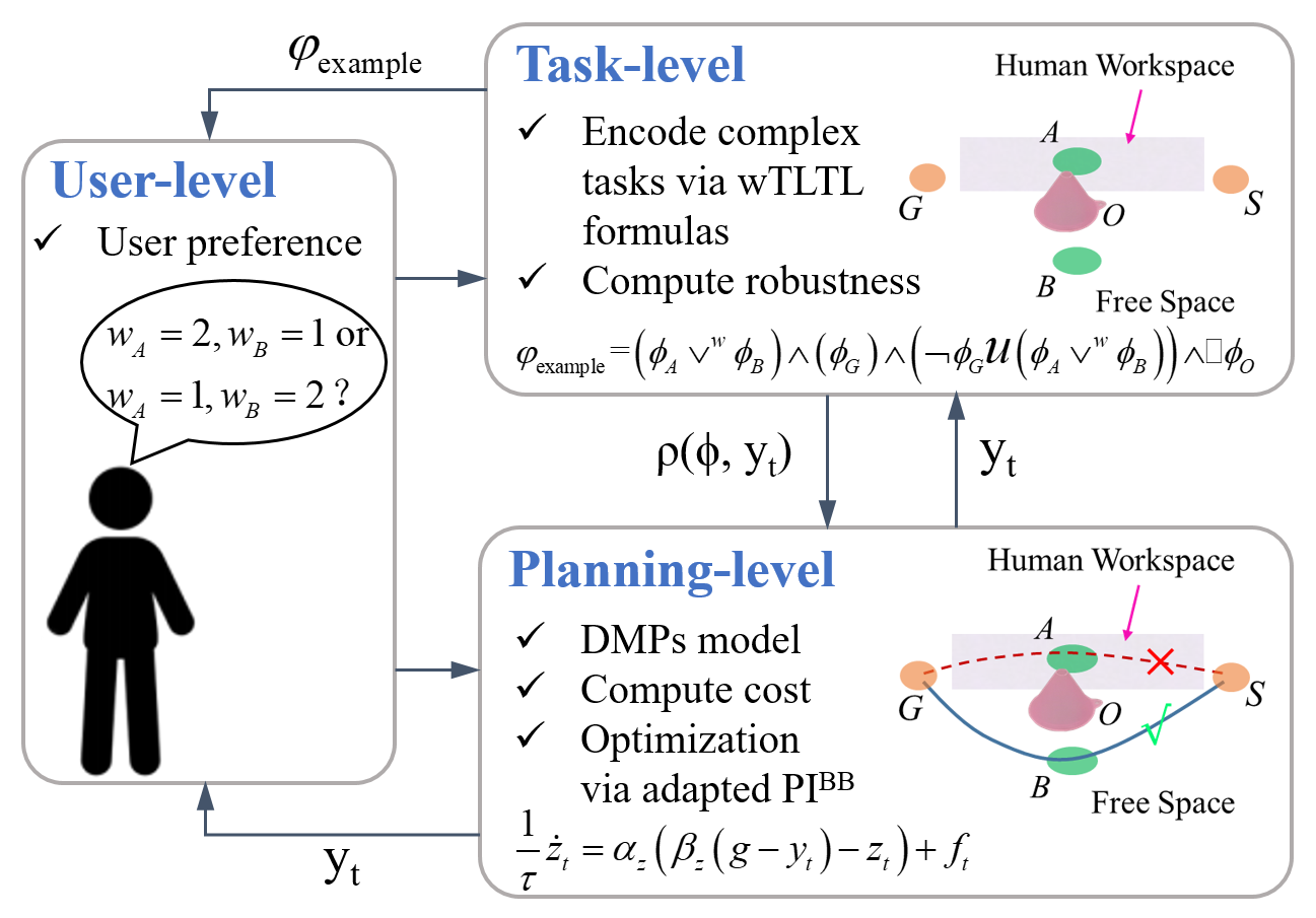
Figure 1: The architecture of $\textrm{P{I}}^{\textrm{BB-TL}}$ for complex manipulation tasks with user preferences. In the task-level, the wTLTL specification encodes the complex manipulation task described in Example 1 and its robustness indicates how well the task is performed. In the planning-level, satisfactory trajectories are generated by optimizing the shape parameters of DMPs via adapted $\textrm{P{I}}^{\textrm{BB}}$ algorithm. User preferences are incorporated in both task and planning levels to indicate the relative importance of subtasks or priorities of alternatives.

To address this motion planning problem, the $\textrm{P{I}}^{\textrm{BB-TL}}$ algorithm is developed. The core idea of $\textrm{P{I}}^{\textrm{BB-TL}}$ is to incorporate DMPs and wTLTL to enable complex manipulations, where wTLTL provides interpretable task specifications to instruct the robot what to do in the task-level, while DMPs are used to generate robot trajectories to instruct the robot how to do in the planning-level. User preferences are further incorporated via wTLTL and the cost function into the task and planning level, respectively, to bias the generated robotic trajectory towards user preferences. The architecture of $\textrm{P{I}}^{\textrm{BB-TL}}$ algorithm is illustrated in Fig. 1.

To elaborate the $\textrm{P{I}}^{\textrm{BB-TL}}$ algorithm, a running example is used throughout this work.

Example 1.

Consider a task that requires the end effector of a manipulator to transport chemical reagent from the initial position $S$ to the reagent rack $G$ in Fig. 2. The manipulator is tasked to visit region $A$ (in human workspace) or $B$ (in free space) before reaching $G$, and do not visit $G$ until $A$ or $B$ is visited, and always avoid obstacle $\mathit{O}$. Such a task can be encoded by a wTLTL formula $\varphi_{example}=\left(\phi_{A}\lor^{w}\phi_{B}\right)\land\phi_{G}\land\left(\lnot\phi_{G}\mathscr{\mathcal{U}}\left(\phi_{A}\lor^{w}\phi_{B}\right)\right)\land\oblong\varphi_{O},$ where $\phi_{A}$, $\phi_{B},$ $\phi_{G}$, $\phi_{O}$ are predicates corresponding to region $\mathit{A}$, $\mathit{B}$, $G$ and $\mathit{O}$, respectively. It is worth pointing out that, for such a complex task $\varphi_{example}$, conventional DMP-based approaches [3, 12] are no longer applicable. There are two main challenges to perform $\varphi_{example}.$ The first challenge is how conventional DMP can be extended to learn optimal shape parameters of motion primitives for complex tasks at a time. Another challenge is how the optimal shape parameters in DMP can be learned while considering user preferences. For instance, suppose there are two feasible plans, i.e., the dashed and solid lines in Fig. 2. Even the path via $A$ to the goal $G$ is shorter, the path via $B$ is more favorable since it avoids human workspace to reduce the potential collision of chemical reagent with human operator. Such a preference should be encoded in the motion planning strategy.

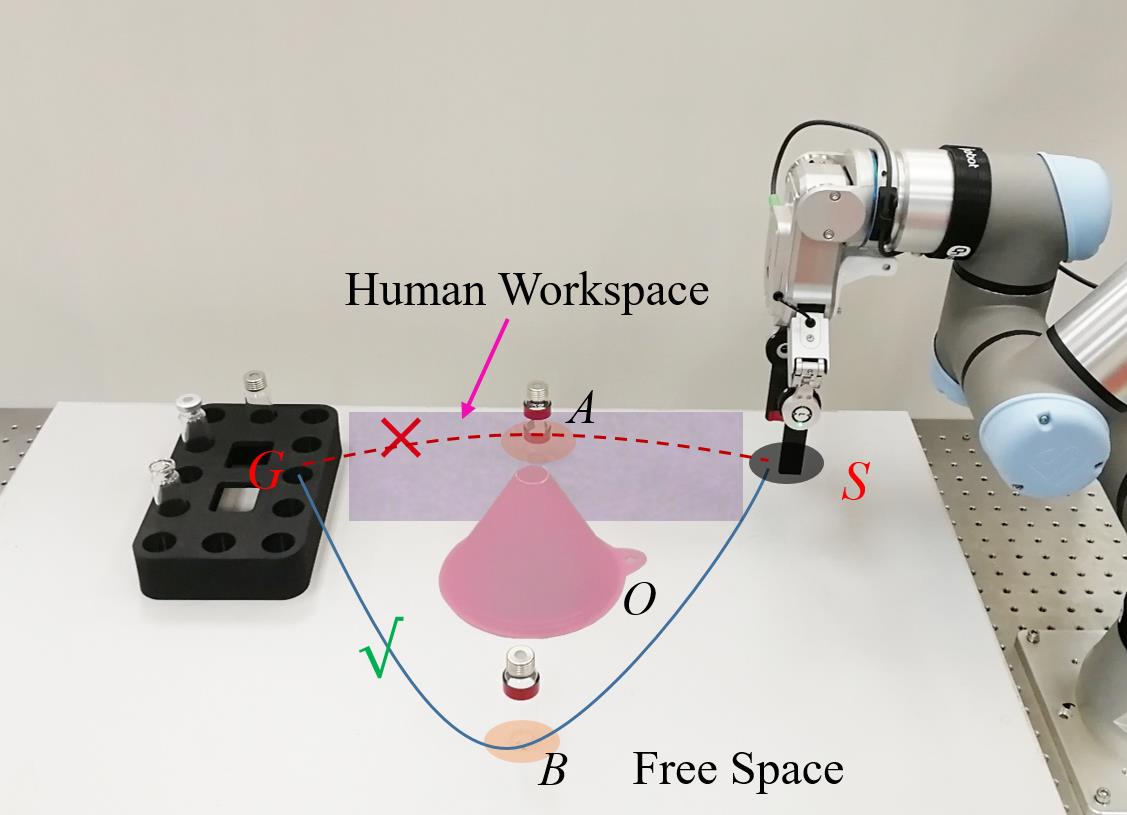
Figure 2: A complex manipulation task with user preference, where $S$ represents the initial position, $G$ represents the goal position, $O$ represents the obstacles. Human workspace is indicated by the shaded area.

IV Cost Function Design and Policy Improvement

This section first presents the cost function design in Sec. IV-A, which exploits wTLTL robustness to guide motion planning for complex tasks. Section IV-B then presents how the black-box optimization algorithm can be adapted to solve the synthesis problem.

IV-A TLTL Robustness Guided Cost Function Design

Due to the soundness property of $\rho^{w}\left(y_{0:t},\varphi\right)$, the goal is to design a cost function $J$ such that minimizing $J$ is equivalent to maximizing the satisfaction degree of the wTLTL specification $\varphi$. Optimization methods can then be employed to identify the optimal shape parameters $\theta^{*}$ that minimize the cost function $J$. However, the traditional robustness only considers satisfaction of a TLTL formula at the most extreme sub-formulas, hindering the optimization to find feasible solutions. To address this issue, inspired by [26, 33], we refine wTLTL robustness by accumulating and averaging the robustness over all sub-formulas.

Definition 2 (Smoothed wTLTL Robustness).

Given a specification $\varphi$ and a state trajectory $y_{t:t+k}$, the smoothed wTLTL robustness $\widetilde{\rho}$ is defined as follows:

$$\widetilde{\rho}\left(y_{t\vcentcolon t+k},\top\right) =\widetilde{\rho}_{max}^{w},$$

$$\widetilde{\rho}\left(y_{t\vcentcolon t+k},f\left(y_{t}\right)<c\right) =c-f\left(y_{t}\right),$$

$$\widetilde{\rho}\left(y_{t\vcentcolon t+k},\lnot\phi\right) =-\widetilde{\rho}\left(y_{t\vcentcolon t+k},\phi\right),$$

$${\color[rgb]{0,0,0}{\color[rgb]{1,0,0}{\color[rgb]{0,0,1}{\color[rgb]{0,0,0}\widetilde{\rho}\left(y_{t\vcentcolon t+k},\Phi\land\Psi\right)}}}} {\color[rgb]{0,0,0}{\color[rgb]{1,0,0}{\color[rgb]{0,0,1}{\color[rgb]{0,0,0}=\tilde{\min}\left(\rho^{w}\left(y_{t\vcentcolon t+k},\Phi\right),\rho^{w}\left(y_{t\vcentcolon t+k},\Psi\right)\right),}}}}$$

$${\color[rgb]{0,0,1}{\color[rgb]{1,0,0}{\color[rgb]{0,0,1}{\color[rgb]{0,0,0}\widetilde{\rho}\left(y_{t\vcentcolon t+k},\Phi\lor\Psi\right)}}}} {\color[rgb]{0,0,1}{\color[rgb]{1,0,0}{\color[rgb]{0,0,1}{\color[rgb]{0,0,0}=\tilde{\max}\left(\rho^{w}\left(y_{t\vcentcolon t+k},\Phi\right),\rho^{w}\left(y_{t\vcentcolon t+k},\Psi\right)\right),}}}}$$

$$\widetilde{\rho}\left(y_{t\vcentcolon t+k},\Square\phi\right) =\underset{t^{{}^{\prime}}\in\left[t,t+k\right)}{\tilde{\min}}\left(\rho^{w}\left(y_{t\vcentcolon t+k},\phi\right)\right),$$ (8)

$$\widetilde{\rho}\left(y_{t\vcentcolon t+k},\lozenge\phi\right) =\underset{t^{{}^{\prime}}\in\left[t,t+k\right)}{\tilde{\max}}\left(\rho^{w}\left(y_{t\vcentcolon t+k},\phi\right)\right),$$

$${\color[rgb]{1,0,0}{\color[rgb]{0,0,1}{\color[rgb]{0,0,0}\widetilde{\rho}\left(y_{t\vcentcolon t+k},\phi\mathcal{U}\psi\right)}}} {\color[rgb]{1,0,0}{\color[rgb]{0,0,1}{\color[rgb]{0,0,0}=\underset{t^{{}^{\prime}}\in\left[t,t+k\right)}{\tilde{\max}}\left(\tilde{\min}\left(\rho^{w}\left(y_{t^{{}^{\prime}}\vcentcolon t+k},\psi\right)\right),\right.}}}$$

$${\color[rgb]{0,0,1}{\color[rgb]{1,0,0}{\color[rgb]{0,0,1}{\color[rgb]{0,0,0}\left.\underset{t^{{}^{\prime\prime}}\in\left[t,t^{{}^{\prime}}\right)}{\tilde{\textrm{min}}}\left(\rho^{w}\left(y_{t^{{}^{\prime\prime}}\vcentcolon t^{{}^{\prime}}},\psi\right)\right)\right),}}}}$$

$$\widetilde{\rho}\left(y_{t\vcentcolon t+k},\phi\mathcal{T}\psi\right) =\underset{t^{{}^{\prime}}\in\left[t,t+k\right)}{\tilde{\max}}\left(\tilde{\min}\left(\rho^{w}\left(y_{t^{{}^{\prime}}\vcentcolon t+k},\psi\right)\right),\right.$$

$$\left.\underset{t^{{}^{\prime\prime}}\in\left[t,t^{{}^{\prime}}\right)}{\tilde{\max}}\left(\rho^{w}\left(y_{t^{{}^{\prime\prime}}\vcentcolon t^{{}^{\prime}}},\psi\right)\right)\right),$$

$${\color[rgb]{1,0,0}{\color[rgb]{0,0,1}{\color[rgb]{0,0,0}\widetilde{\rho}\left(y_{t\vcentcolon t+k},\phi\mathcal{\Rightarrow}\psi\right)}}} {\color[rgb]{1,0,0}{\color[rgb]{0,0,1}{\color[rgb]{0,0,0}=\tilde{\max}\left(-\rho^{w}\left(y_{t\vcentcolon t+k},\phi\right),\rho^{w}\left(y_{t\vcentcolon t+k},\psi\right)\right).}}}$$

where $\Phi=\land^{w}\phi_{i}$ and $\Psi=\lor^{w}\psi_{i}$.

In Def. 2, $\tilde{\min}$ and $\tilde{\max}$ are smoothed version of the conventional $\min$ and $\max$ operators which are calculated by (6) and (7) as discussed in Section II-C.

Theorem 1.

Given a wTLTL specification $\varphi$ and a state trajectory $y_{t:t+k}$, for any pre-defined error bound $\epsilon>0$, there exist $\overline{k}_{1}$ and $\overline{k}_{2}$ such that $0\leq\rho^{w}\left(y_{t:t+k},\varphi\right)-\widetilde{\rho}\left(y_{t:t+k},\varphi\right)\leq\epsilon$ for all $k_{1}\geq\bar{k}_{1}$, $k_{2}\geq\bar{k}_{2}$, where $k_{1}$ and $k_{2}$ are tuning parameters defined in (6) and (7).

The proof of Theorem 1 is omitted, since it is a trivial extension of Theorem 2 in [33]. Theorem 1 indicates that the smoothed wTLTL robustness $\widetilde{\rho}$ is an under-approximation of $\rho^{w}$, and thus it provides a sufficient condition for the satisfaction check of wTLTL specification $\varphi$. That is, if $\widetilde{\rho}\left(y_{t:t+k},\varphi\right)>0$, it is always true that $\rho^{w}\left(y_{t:t+k},\varphi\right)>0$, which implies $y_{t:t+k}\vDash\varphi$. Theorem 1 also indicates that the smoothed wTLTL robustness $\widetilde{\rho}$ gradually approaches the true robustness $\mathit{\rho}$ as $k_{1}$ and $k_{2}$ increase, which means that the approximation will not hide any potential solutions if $k_{1}$ and $k_{2}$ are sufficiently large.

By Theorem 1, we design the cost function $J$ as

$$J\left(\widetilde{\rho}\left(y_{0:t},\varphi\right)\right)=\left\{\begin{array}[]{cc}-\widetilde{\rho}\left(y_{0:t},\varphi\right),&\text{ if }\widetilde{\rho}\left(y_{0:t},\varphi\right)<0,\\ 0,&\text{otherwise,}\end{array}\right.$$ (9)

which indicates that minimizing the cost function (i.e., $J\left(\widetilde{\rho}\left(y_{0:t},\varphi\right)\right)\rightarrow 0$) can lead to $\widetilde{\rho}\left(y_{0:t},\varphi\right)\geq 0$, resulting in that $y_{0:t}\vDash\varphi$ due to the soundness property of wTLTL robustness.

Based on (9), the problem considered in Sec. III can then be formally formulated as

$$\theta^{\ast} =\underset{\theta}{\textrm{argmin}}J\left(\widetilde{\rho}\left(y_{0:t},\varphi\right)\right),$$ (10)

s.t. $$\;(\ref{eq:DMP})\text{ are satisfied},$$

where the constraint $y_{0:t}\left(y_{0},g,\theta^{\ast}\right)\vDash\varphi$ is implicitly encoded in the the cost function $J$ via the smoothed wTLTL robustness. Note that the goal of (10) is to identify a satisfactory trajectory, rather than an optimal trajectory with largest robustness, with respect to logical and temporal specifications and user preferences. Ongoing research is to leverage the wTLTL robustness in the design of the cost function to facilitate the identification of the optimal trajectory.

IV-B TLTL Guided Black-Box Optimization

After designing the optimization problem in (10), the next step is to identify the optimal shape parameters $\theta^{*}$ with respect to $J$. Two widely used approaches to perform this optimization are reinforcement learning (RL) and black-box optimization (BBO). As discussed in [1] and [34], $\textrm{P{I}}^{\textrm{2}}$ is a RL algorithm which uses reward information during exploratory policy executions, while $\textrm{P{I}}^{\textrm{BB}}$, a variant of $\textrm{P{I}}^{\textrm{2}}$ with constant exploration and without temporal averaging, is a BBO algorithm that uses the total reward during execution, which enables that the utility function can be treated as a black box. Despite the lack of theoretical guarantees, strong empirical evidence shows that $\textrm{P{I}}^{\textrm{BB}}$ has equal or superior performance than $\textrm{P{I}}^{\textrm{2}}$ in terms of convergence speed and robustness of policy improvement. In addition, as a special case of covariance matrix adaptation evolutionary strategy, $\textrm{P{I}}^{\textrm{BB}}$ is a global optimization method[34, 35].

Algorithm 1 wTLTL Guided $\textrm{P{I}}^{\textrm{BB-TL}}$ Algorithm for DMPs

1:procedure Input: (the initial shape parameter $\theta^{init}$; the wTLTL specification $\varphi$; the exploration levels $\lambda^{init}$, $\lambda^{min}$, and $\lambda^{max}$; the sample size $M$; the eliteness parameter $h$) Output: the optimal shape parameters $\theta^{*}$ Initialization: set $\theta=\theta^{init}$ , $\Sigma=\lambda^{init}I$

2:    while cost $J\left(\widetilde{\rho}\left(y_{0:t},\varphi\right)\right)$ not converged do

3:       Exploration: sample parameters and compute costs

4:       for  each $m\in M$  do

5:          $\theta_{m}\sim\mathcal{N}\left(\theta,\Sigma\right)$

6:          Generate a trajectory $y_{0:t}^{m}$ based on current $\theta_{m}$ according to (1)

7:          Compute the $\widetilde{\rho}\left(y_{0:t}^{m},\varphi\right)$ according to Def. 1 and Def. 2

8:          Compute the cost $J_{m}$ according to (9)

9:       end for

10:       $J^{min}=\textrm{min}\left\{J_{m}\right\}_{m=1}^{M}$

11:       $J^{max}=\textrm{max}\left\{J_{m}\right\}_{m=1}^{M}$

12:       Evaluation: compute weight for each sample

13:       for  each $m\in M$  do

14:          $P_{m}=\frac{exp\left(-h\frac{J_{m}-J^{min}}{J^{max}-J^{min}}\right)}{\sum_{l=1}^{M}exp\left(-h\frac{J_{l}-J^{min}}{J^{max}-J^{min}}\right)}$

15:       end for

16:       Update: weighted averaging over $M$ samples

17:       $\Sigma\leftarrow\sum_{m=1}^{M}\left[P_{m}\left(\theta_{m}-\theta\right)\left(\theta_{m}-\theta\right)^{T}\right]$

18:       $\Sigma^{new}\leftarrow\textrm{boundcovar}\left(\Sigma,\lambda^{min},\lambda^{max}\right)$

19:       $\theta^{new}\leftarrow\stackrel{{\scriptstyle[}}{{m}}=1]{M}{\sum}\left[P_{m}\theta_{m}\right]$

20:    end while

21:end procedure

Motivated by the discussion above, this section presents how the stochastic optimization algorithm $\textrm{P{I}}^{\textrm{BB}}$ can be adapted in our $\textrm{P{I}}^{\textrm{BB-TL}}$ to solve the optimization problem in (10). Specifically, the $\textrm{P{I}}^{\textrm{BB-TL}}$ algorithm is outlined in Alg. 1, and the shape parameters are updated following the subsequent steps:

1. Initialization (line 1): Set the mean and covariance $\left\langle\theta,\Sigma\right\rangle$ to $\left\langle\theta^{init},\lambda^{init}I\right\rangle$, where $I$ is an identity matrix with appropriate dimension.

2. Exploration (line 3-9): Sample $M$ parameter vectors $\theta_{m}$, $m=1,\ldots M$, from $\mathcal{N}\left(\theta,\Sigma\right)$ according to $\left\{\theta_{m}=\theta+\epsilon_{m}\right\}_{m=1}^{M}$, where $\epsilon_{m}$ is sampled from a zero-mean Gaussian distribution with variance $\Sigma$. Compute the cost $J_{m}=J\left(\widetilde{\rho}\left(y_{0:t},\varphi\right)\right)$ of each sample.

3. Evaluation (line 10-15): Compute the weight $P\in\mathbb{R}^{M}$ for the $M$ samples, where the $m$th entry $P_{m}\in\left[0,1\right]$ and $\sum_{m=1}^{M}P_{m}=1$. Specifically, using the normalized exponentiation function, $P_{m}$ is computed as

   $$\begin{array}[]{c}P_{m}=\frac{\exp\left(-h\frac{J_{m}-J^{min}}{J^{max}-J^{min}}\right)}{\sum_{r=1}^{M}\exp\left(-h\frac{J_{r}-J^{min}}{J^{max}-J^{min}}\right)},\end{array}$$ (11)

   where $J^{min}=\textrm{min}\left\{J_{m}\right\}_{m=1}^{M}$, $J^{max}=\textrm{max}\left\{J_{m}\right\}_{m=1}^{M}$, and $h$ is the eliteness parameter. If a large $h$ is used, only a few samples will contribute to the weighted averaging. If $h=0$, no learning would occur since all given samples have equal weight independent of the cost. In general, low-cost samples have higher weights, and vice versa.

4. Update (line 16-19): Update the parameters $\left\langle\theta,\Sigma\right\rangle$ to $\left\langle\theta^{new},\Sigma^{new}\right\rangle$ with weighted averaging according to

   $$\Sigma^{new}\leftarrow\textrm{boundcovar}\left(\Sigma,\lambda^{min},\lambda^{max}\right)$$ (12)

   and

   $$\theta^{new}=\stackrel{{\scriptstyle[}}{{m}}=1]{M}{\sum}\left[P_{m}\theta_{m}\right],$$ (13)

   where

   $$\Sigma=\stackrel{{\scriptstyle[}}{{m}}=1]{M}{\sum}\left[P_{m}\left(\theta_{m}-\theta\right)\left(\theta_{m}-\theta\right)^{T}\right]$$ (14)

   and $\textrm{boundcovar}\left(\Sigma,\lambda^{min},\lambda^{max}\right)$ is a function that restricts the eigenvalues $\lambda$ of the covariance matrix $\Sigma$ within $\left[\lambda^{min},\lambda^{max}\right]$, i.e., if $\lambda<\lambda^{min}$, then $\lambda=\lambda^{min}$; if $\lambda>\lambda^{max}$, then $\lambda=\lambda^{max}$. The low-cost samples contribute more to the update since they have higher weights, leading to that $\theta$ moves towards its optimum $\theta^{\ast}$.

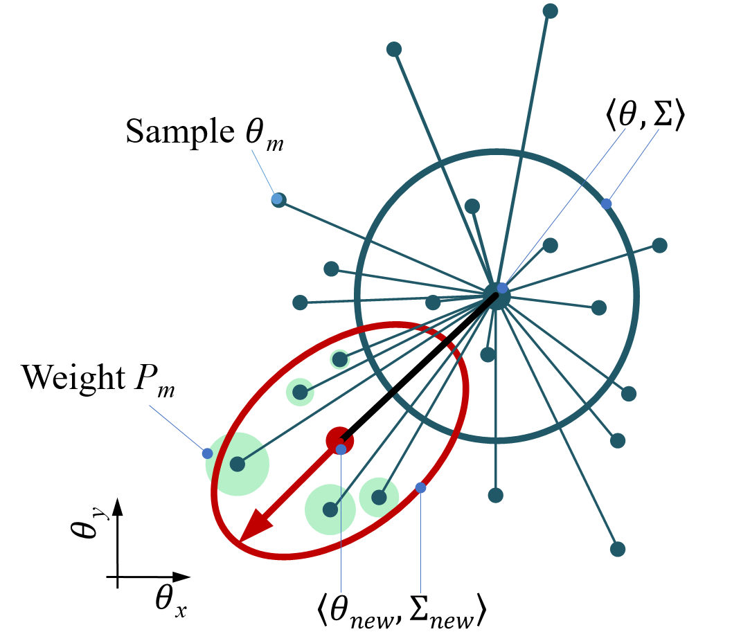
Figure 3: Visualization of one parameter update using $\textrm{P{I}}^{\textrm{BB-TL}}$ in a 2-D search space. Sampling $M$ parameter vectors when the current parameter $\theta$ has not converged to the optimum $\theta^{*}$. The samples closer to $\theta^{*}$ have larger weights (visualized as green circles) than those further away from $\theta^{*}$. Since the new parameters are weighted, the mean $\theta$ moves in the direction towards the high-weight and low-cost samples during the update, so that $\mathit{\theta}$ moves closer to $\theta^{*}$.

The visualization of one parameter update using $\textrm{P{I}}^{\textrm{BB-TL}}$ in a 2-D search space is shown in Fig. 3. We sample $M$ parameter vectors when the current parameter $\theta$ has not converged to the optimum $\theta^{*}$. The samples closer to $\theta^{*}$ have larger weights (visualized as green circles) than those further away from $\theta^{*}$. Since the new parameters are weighted, the mean $\theta$ moves in the direction towards the high-weight and low-cost samples during the update, so that $\mathit{\theta}$ moves closer to $\theta^{*}$. The same idea applies to the covariance matrix. When the parameters update, its maximum eigenvalue $\mathit{\lambda}$ of the covariance matrix increases, which results in an elongated covariance matrix such that the eigenvector points towards the direction of $\theta^{*}$ (visualized as an arrow). Following the steps above until $J_{m}\rightarrow 0$, the optimal $\theta^{\ast}$ can be obtained, which in turn yields a trajectory $y_{0:t}$ that satisfies the wTLTL specifications $\varphi$. Given that the sample size is $M$ and the number of updates required for cost convergence is $\varLambda$, the computational complexity of $\textrm{P{I}}^{\textrm{BB-TL}}$ is $O(\varLambda M)$ according to Alg. 1.

V Case Studies

In this section, the developed temporal logic guided $\textrm{P{I}}^{\textrm{BB-TL}}$ algorithm is implemented in Python 3.5 on Ubuntu 16.04. To validate the effectiveness of our approach, we first carry out two simulations on a Mac with 3.40 GHz Intel Xeon E-2224 CPU and 16 GB RAM, and then validate this approach in a real-world case using Universal Robot UR5e.

V-A Simulation Results

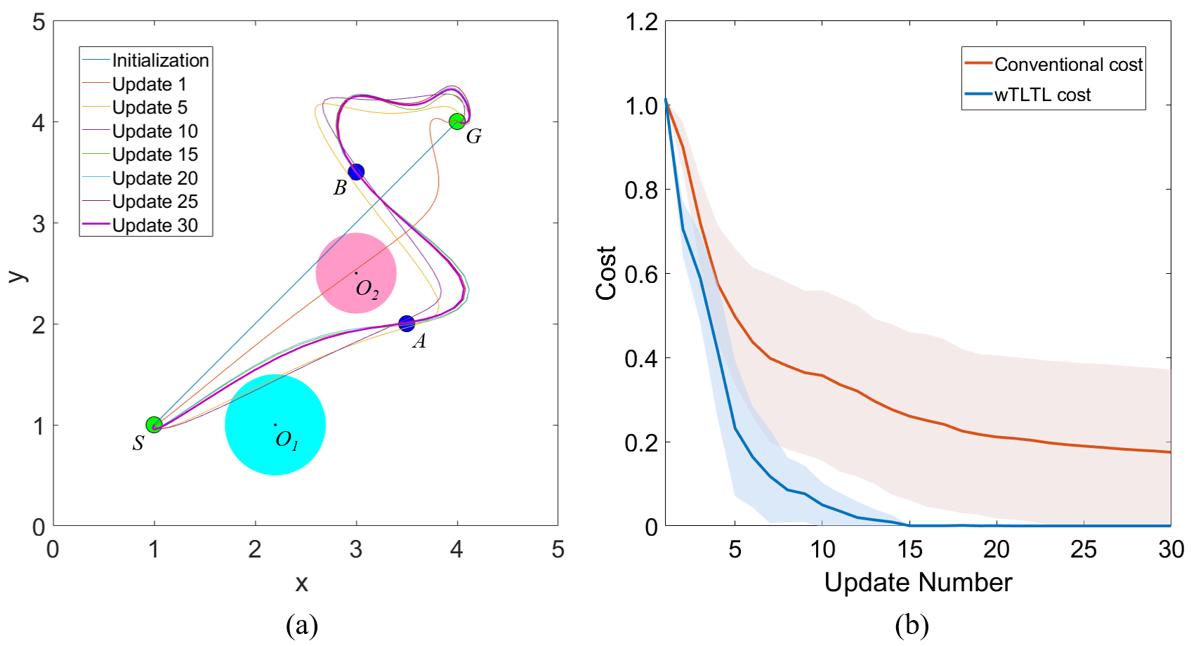
Figure 4: (a) The evolution of generated trajectories using $\textrm{P{I}}^{\textrm{BB-TL}}$ algorithm in Case 1 for a sequential goal reaching task with obstacle avoidance. (b) Learning curves of the wTLTL guided cost and the conventional cost trained with $\textrm{P{I}}^{\textrm{BB}}$ in Case 1, respectively. The solid line shows the mean of the cost and the shaded area represents the corresponding standard deviation of 20 training results.

Consider a 2-D system whose motion is described by the DMPs in (1). The developed wTLTL guided $\textrm{P{I}}^{\textrm{BB-TL}}$ algorithm is implemented to optimize the shape parameters $\theta$ of DMPs. The parameters of $\textrm{P{I}}^{\textrm{BB-TL}}$ are set as follows. The initial shape parameters vector $\theta^{init}$ is a zero vector. The initial, minimum, and maximum exploration are set to $\lambda^{init}=0.05$, $\lambda^{min}=0.05$, $\lambda^{max}=None$, respectively. The number of trials per update is set to $\Gamma=20$, the number of basis functions for 1-D DMP $\kappa=10$, the eliteness parameter is set to $h=10$.

Case 1: In this case, to show the capability of generating trajectories for complex manipulations, the conventional cost function from [12] is treated as a baseline and compared with the developed wTLTL guided cost function. Specifically, we consider a sequential goal reaching task, in which, as shown in Fig. 4, the robot is required to go from $S$ to $G$, and sequentially visit $A$ and $B$ while avoiding obstacles $O_{1}$ and $O_{2}$. Such a complex task can be formulated using wTLTL specification as

$$\varphi_{case1}=\left(\phi_{A}\mathcal{T}\phi_{B}\right)\land\left(\lnot\phi_{B}\mathcal{U}\phi_{A}\right)\land\oblong\varphi_{O},$$ (15)

where $\varphi_{O}=\wedge_{i=1,2}d_{O_{i}}>r_{O_{i}}$ with $d_{O_{i}}$ representing the Euclidean distance between the robot and the obstacle $O_{i}$ and $r_{O_{i}}$ representing the radius of obstacle $O_{i}$. In English, $\varphi_{case1}$ means “visit $A$ then $B$, do not visit $B$ until $A$ is visited, and always avoid the obstacles $O_{1}$ and $O_{2}$”.

Since conventional cost function cannot deal with user preferences, to be a fair comparison, the user preferences in wTLTL guided cost function are not considered in this case, i.e., we set all weights $w_{i}=1,$ $\forall i\in\left\{1,\ldots,N\right\}$ in implementation. The smoothed wTLTL robustness and cost function of $\textrm{P{I}}^{\textrm{BB-TL}}$ can be obtained by following (8) and (9), respectively. Following the design in [12], the conventional cost function is adapted to the particular task $\varphi_{case1}$ as

$$\bar{J}=-c_{1}J_{O}+c_{2}J_{G}$$ (16)

where $c_{1},c_{2}\in\mathbb{R}^{+}$ are relative weights, i.e. $c_{1}=0.6$, $c_{2}=0.5$. In (16), $J_{O}=\sum_{i=1,2}(d_{O_{i}}-r_{O_{i}})$ where $d_{O_{i}}-r_{O_{i}}=0$ if $d_{O_{i}}>r_{O_{i}}$, and $J_{G}=d_{A}+d_{B}$ where $d_{A}$ and $d_{B}$ are the Euclidean distance between the robot and the region $A$ and $B$, respectively.

The average learning time for the shape parameters $\theta\in\mathit{\mathbb{R}^{\textrm{10}}}$ of DMPs with respect to the conventional cost function and the wTLTL guided cost function are $7.89$s and $6.94$s, respectively. Fig. 4 (a) shows the generated trajectories after updates using $\textrm{P{I}}^{\textrm{BB-TL}}$, which indicates $\varphi_{case1}$ is successfully completed. The evolution of the costs are shown in Fig. 4 (b), which indicates that the wTLTL guided cost function outperforms the conventional cost function in the sense that the cost converges faster.

Figure 5: Simulated trajectories of $\varphi_{case2}$ with $w_{A}=2,w_{B}=1$ in (a) and $w_{A}=1,w_{B}=2$ in (b).

Case 2: To show the capability of handling user preferences in $\textrm{P{I}}^{\textrm{BB-TL}}$, we consider a similar case in [26]. This case considers a task that requires the robot to visit region $A$ or $B$, then visit region $G$, and do not visit $G$ until either $A$ or $B$ is visited, while always avoiding obstacle $O$, as shown in in Fig. 5. Such a task can be written in wTLTL formula as

$$\varphi_{case2}=\left(\phi_{A}\lor^{w}\phi_{B}\right)\land\phi_{G}\land\left(\lnot\phi_{G}\mathscr{\mathcal{U}}\left(\phi_{A}\lor^{w}\phi_{B}\right)\right)\land\oblong\varphi_{O},$$ (17)

where $\varphi_{O}=d_{O}>r_{O}$, $d_{O}$ is the Euclidean distance between the trajectory and obstacle $O$, $r_{O}$ is the radius of obstacle $O_{i}$.

The task $\varphi_{case2}$ indicates that the goal $G$ can be reached by a path that traverses either region $A$ or $B$. To reflect the user preferences, $w_{A}$ and $w_{B}$ are used to indicate the weights about which path is more preferred, i.e., region $A$ is preferred if $w_{A}>w_{B}$ and region $B$ is preferred otherwise. The weights are normalized by $\bar{w_{i}}=\frac{w_{i}}{\sum_{j=1}^{N}w_{j}}$. The wTLTL robustness and the cost function are then obtained following the methods in Section IV, and then optimized using $\textrm{P{I}}^{\textrm{BB-TL}}$. The generated trajectories are shown in Fig. 5 (a) and (b), and the learning times are $7.97\textrm{s}$ and $8.04\textrm{s}$, respectively. It is clear from Fig. 5 that user preferences can be incorporated in trajectory generation, i.e., regions with higher priority (importance) are likely to be visited if higher disjunction (conjunction) aggregator weights are assigned accordingly.

V-B Experimental Results

Figure 6: Snapshots of a manipulation task with complex logic and temporal constraints. The end effector of UR5e transports chemical reagent from $S$ to the reagent rack $\mathit{G}$ via region $B$ with user preference.

To evaluate practical performance, the developed $\textrm{P{I}}^{\textrm{BB-TL}}$ is validated on a physical UR5e robot in a 3D workspace, which includes 2D trajectory planning and following and 3D grasp/release actions. The 2D trajectory is generated offline using $\textrm{P{I}}^{\textrm{BB-TL}}$ with user preferences and temporal logic constraints, while the grasp/release actions are performed in the 3D workspace following embedded library functions. The experimental layout is shown in Example 1 and the task to be performed by the manipulator is the same as $\varphi_{case2}$ in (17). Following Section IV, the wTLTL robustness and the cost function with user preference can be obtained. By setting a larger weight, a trajectory that passes region $\mathit{B}$ can be trained via Alg. 1 offline. Such a path reflects the user’s preference on safety, i.e., prefer to avoid human workspace when carrying chemical reagent, but with the cost of traveling a longer path to reach the goal $G$. Fig. 6 shows the snapshots of the motion of the end effector of the UR5e manipulator, which indicates that the end effector first goes to region $\mathit{B}$ from $\mathit{S}$ to grasp the chemical reagent with user preference and then transports it to the reagent rack $\mathit{G}$ while avoiding obstacle $\mathit{O}$. The experiment video is provided.

V-C Discussions

As indicated by the simulation results, the wTLTL guided cost function outperforms the conventional cost function, mainly due to the incorporation of temporal logic in the design of DMPs. Since the sequential goal reaching task can also be solved by the $\textrm{P{I}}^{\textrm{2}}$SEQ algorithm in [12], the performance of $\textrm{P{I}}^{\textrm{2}}$SEQ and $\textrm{P{I}}^{\textrm{BB-TL}}$ are compared. Table I shows, under the same conditions, the number of DMPs and the number of optimization parameters required in Case 1, Case 2 and UR5e experiment for $\textrm{P{I}}^{\textrm{2}}$SEQ and $\textrm{P{I}}^{\textrm{BB-TL}}$, respectively. Given a $n$-goal-reaching task in a $\eta$-D space with $\kappa$ basis functions, $\eta n$ DMPs with $\eta n\kappa$ weight parameters need to be trained using $\textrm{P{I}}^{\textrm{2}}$SEQ while only $\eta$ DMPs with $\eta\kappa$ weight parameters are needed using $\textrm{P{I}}^{\textrm{BB-TL}}$ to generate a satisfactory trajectory. Therefore, $\textrm{P{I}}^{\textrm{BB-TL}}$ is more efficient in the sense that less parameters need to be trained. In addition, due to the resemblance to human natural language, the employment of temporal logic significantly increases the interpretability of the cost function in DMPs. That is, complex tasks can be conveniently formulated in temporal logic specifications and then encoded in the cost function of DMPs to facilitate the generation of satisfactory trajectories. Such an advantage is not available in the conventional DMP-based methods. Moreover, by using wTLTL, our approach can further incorporate user preferences in the trajectory generation, which has less been considered in many existing DMP-based methods. It is worth mentioning that, as a special case of covariance matrix adaptation evolutionary strategy, $\textrm{P{I}}^{\textrm{BB-TL}}$ is a global optimization method [34, 35] while $\textrm{P{I}}^{\textrm{2}}$SEQ is a gradient-based method and may converge to a local optimum.

TABLE I: Comparison of the number of DMPs and the number of optimization parameters using $\textrm{P{I}}^{\textrm{2}}$SEQ and $\textrm{P{I}}^{\textrm{BB-TL}}$

	Number of DMPs			Number of Parameters
	Case 1	Case 2	UR5e	Case 1	Case 2	UR5e
$\textrm{P{I}}^{\textrm{2}}$SEQ	6	4	4	60	40	40
$\textrm{P{I}}^{\textrm{BB-TL}}$	2	2	2	20	20	20

VI Conclusion

A temporal logic guided $\textrm{P{I}}^{\textrm{BB-TL}}$ algorithm is developed in this work to generate desired motions for complex manipulation tasks with user preferences. The integration of wTLTL not only enables the encoding of complex tasks that involve a sequence of logically organized action plans with user preferences, but also provides a convenient and efficient means to design the cost function. The black-box optimization is adapted to identify optimal shape parameters of DMPs to enable motion planning of robotic systems. Simulation and experiment demonstrate its success in handling complex manipulations; however, current research mainly focus on motion generation in static environments. Ongoing research will consider online adaptive optimization and reactive temporal logic planning to extend $\textrm{P{I}}^{\textrm{BB-TL}}$ to dynamic workspace with mobile obstacles and time-varying missions.

References

- [1] K. Chatzilygeroudis, V. Vassiliades, F. Stulp, S. Calinon, and J.-B. Mouret, “A survey on policy search algorithms for learning robot controllers in a handful of trials,” IEEE Trans. Robot., vol. 36, no. 2, pp. 328–347, 2020.
- [2] S. Schaal, “Dynamic movement primitives-a framework for motor control in humans and humanoid robotics,” in Adaptive motion of animals and machines. Springer, 2006, pp. 261–280.
- [3] C. L. Bottasso, D. Leonello, and B. Savini, “Path planning for autonomous vehicles by trajectory smoothing using motion primitives,” IEEE Trans. Control Syst. Technol., vol. 16, no. 6, pp. 1152–1168, 2008.
- [4] S. Dutta, L. Behera, and S. Nahavandi, “Skill learning from human demonstrations using dynamical regressive models for multitask applications,” IEEE Trans. Syst., Man, Cybern., Syst., 2018.
- [5] M. Raković, B. Borovac, M. Nikolić, and S. Savić, “Realization of biped walking in unstructured environment using motion primitives,” IEEE Trans. Robot., vol. 30, no. 6, pp. 1318–1332, 2014.
- [6] A. Colomé and C. Torras, “Dimensionality reduction for dynamic movement primitives and application to bimanual manipulation of clothes,” IEEE Trans. Robot., vol. 34, no. 3, pp. 602–615, 2018.
- [7] A. Gams, B. Nemec, A. J. Ijspeert, and A. Ude, “Coupling movement primitives: Interaction with the environment and bimanual tasks,” IEEE Trans. Robot., vol. 30, no. 4, pp. 816–830, 2014.
- [8] A. J. Ijspeert, J. Nakanishi, H. Hoffmann, P. Pastor, and S. Schaal, “Dynamical movement primitives: learning attractor models for motor behaviors,” Neural Comput, vol. 25, no. 2, pp. 328–373, 2013.
- [9] J. Peters and S. Schaal, “Reinforcement learning of motor skills with policy gradients,” J. Neural Netw., vol. 21, no. 4, pp. 682–697, 2008.
- [10] ——, “Policy gradient methods for robotics,” in Proc. IEEE/RSJ Int. Conf. Intell. Robots. IEEE, 2006, pp. 2219–2225.
- [11] C. Daniel, G. Neumann, O. Kroemer, J. Peters et al., “Hierarchical relative entropy policy search,” J. Mach. Learn. Res., vol. 17, pp. 1–50, 2016.
- [12] F. Stulp, E. A. Theodorou, and S. Schaal, “Reinforcement learning with sequences of motion primitives for robust manipulation,” IEEE Trans Robot, vol. 28, no. 6, pp. 1360–1370, 2012.
- [13] E. Theodorou, J. Buchli, and S. Schaal, “A generalized path integral control approach to reinforcement learning,” J. Mach. Learn. Res., vol. 11, pp. 3137–3181, 2010.
- [14] F. Stulp and P.-Y. Oudeyer, “Proximodistal exploration in motor learning as an emergent property of optimization,” Dev. Sci., vol. 21, no. 4, p. e12638, 2018.
- [15] S. Calinon, “A tutorial on task-parameterized movement learning and retrieval,” Intelligent service robotics, vol. 9, no. 1, pp. 1–29, 2016.
- [16] C. Baier and J.-P. Katoen, Principles of model checking. MIT press, 2008.
- [17] M. Kloetzer and C. Mahulea, “LTL-based planning in environments with probabilistic observations,” IEEE Trans. Autom. Sci. Eng., vol. 12, no. 4, pp. 1407–1420, 2015.
- [18] M. Cai, H. Peng, Z. Li, and Z. Kan, “Learning-based probabilistic LTL motion planning with environment and motion uncertainties,” IEEE Trans. Autom. Control, vol. 66, no. 5, pp. 2386–2392, 2020.
- [19] M. Cai, S. Xiao, B. Li, Z. Li, and Z. Kan, “Reinforcement learning based temporal logic control with maximum probabilistic satisfaction,” in Proc. Int. Conf. Robot. Autom. Xi’an, China: IEEE, 2021, pp. 806–812.
- [20] M. Cai, M. Hasanbeig, S. Xiao, A. Abate, and Z. Kan, “Modular deep reinforcement learning for continuous motion planning with temporal logic,” IEEE Robot. Autom. Lett., vol. 6, no. 4, pp. 7973–7980, 2021.
- [21] A. K. Bozkurt, Y. Wang, M. M. Zavlanos, and M. Pajic, “Control synthesis from linear temporal logic specifications using model-free reinforcement learning,” in Int. Conf. Robot. Autom., 2020, pp. 10 349–10 355.
- [22] O. Maler and D. Nickovic, “Monitoring temporal properties of continuous signals,” in Proc. Formal Techn. Model. Anal. Timed Fault Tolerant Syst. Springer, 2004, pp. 152–166.
- [23] S. Saha and A. A. Julius, “An milp approach for real-time optimal controller synthesis with metric temporal logic specifications,” in Proc. IEEE Amer. Control Conf., 2016, pp. 1105–1110.
- [24] V. Raman, A. Donzé, M. Maasoumy, R. M. Murray, A. Sangiovanni-Vincentelli, and S. A. Seshia, “Model predictive control with signal temporal logic specifications,” in Proc. IEEE Conf. Decis. Control, 2014, pp. 81–87.
- [25] C. Belta and S. Sadraddini, “Formal methods for control synthesis: An optimization perspective,” Annu. Rev. Control Robot. Auton. Syst.,, vol. 2, pp. 115–140, 2019.
- [26] N. Mehdipour, C. I. Vasile, and C. Belta, “Specifying user preferences using weighted signal temporal logic,” IEEE Control Syst. Lett., vol. 5, no. 6, pp. 2006–2011, 2021.
- [27] A. G. Puranic, J. V. Deshmukh, and S. Nikolaidis, “Learning from demonstrations using signal temporal logic in stochastic and continuous domains,” IEEE Robot. Autom. Lett., vol. 6, no. 4, pp. 6250–6257, 2021.
- [28] T. Latvala, A. Biere, K. Heljanko, and T. Junttila, “Simple bounded ltl model checking,” in Int. Conf. Form. Method. Computer-Aided Des. Springer, 2004, pp. 186–200.
- [29] G. De Giacomo and M. Y. Vardi, “Linear temporal logic and linear dynamic logic on finite traces,” in Proc. Int. Jt. Conf. Artif. Intell. Association for Computing Machinery, 2013, pp. 854–860.
- [30] X. Li, C.-I. Vasile, and C. Belta, “Reinforcement learning with temporal logic rewards,” in IEEE Int. Conf. Intell. Robot. Syst., 2017, pp. 3834–3839.
- [31] X. Li, Z. Serlin, G. Yang, and C. Belta, “A formal methods approach to interpretable reinforcement learning for robotic planning,” Sci. Robot., vol. 4, no. 37, 2019.
- [32] C. Innes and R. Ramamoorthy, “Elaborating on learned demonstrations with temporal logic specifications,” in Robot.: Sci. Syst., 2020.
- [33] Y. Gilpin, V. Kurtz, and H. Lin, “A smooth robustness measure of signal temporal logic for symbolic control,” IEEE Control Syst. Lett., vol. 5, no. 1, pp. 241–246, 2020.
- [34] F. Stulp and O. Sigaud, “Policy improvement methods: Between black-box optimization and episodic reinforcement learning,” 2012.
- [35] N. Hansen and A. Ostermeier, “Completely derandomized self-adaptation in evolution strategies,” Evolutionary computation, vol. 9, no. 2, pp. 159–195, 2001.