Cartesian Tree Subsequence Matching

Abstract

Park et al. [TCS 2020] observed that the similarity between two (numerical) strings can be captured by the Cartesian trees: The Cartesian tree of a string is a binary tree recursively constructed by picking up the smallest value of the string as the root of the tree. Two strings of equal length are said to Cartesian-tree match if their Cartesian trees are isomorphic. Park et al. [TCS 2020] introduced the following Cartesian tree substring matching (CTMStr) problem: Given a text string $T$ of length $n$ and a pattern string of length $m$, find every consecutive substring $S=T[i..j]$ of a text string $T$ such that $S$ and $P$ Cartesian-tree match. They showed how to solve this problem in $\tilde{O}(n+m)$ time. In this paper, we introduce the Cartesian tree subsequence matching (CTMSeq) problem, that asks to find every minimal substring $S=T[i..j]$ of $T$ such that $S$ contains a subsequence $S^{\prime}$ which Cartesian-tree matches $P$. We prove that the CTMSeq problem can be solved efficiently, in $O(mnp(n))$ time, where $p(n)$ denotes the update/query time for dynamic predecessor queries. By using a suitable dynamic predecessor data structure, we obtain $O(mn\log\log n)$-time and $O(n\log m)$-space solution for CTMSeq. This contrasts CTMSeq with closely related order-preserving subsequence matching (OPMSeq) which was shown to be NP-hard by Bose et al. [IPL 1998].

1 Introduction

A time series is a sequence of events which can be represented by symbols or numbers in many cases. An episode is a collection of events which occur in a short time period. The episode matching problem asks to find every minimal substring $S=T[i..j]$ of a text $T$ such that a pattern $P$ is a (non-consecutive) subsequence of $S$. Let $n$ and $m$ be the lengths of the text $T$ and the pattern $P$, respectively. There exists a naïve $O(mn)$-time $O(1)$-space algorithm for episode matching, which scans the text back and forth. In 1997, Das et al. [7] presented a weakly subquadratic $O(mn/\log m)$-time $O(m)$-space algorithm for episode matching. Very recently, Bille et al. [3] showed that even a simpler version of episode matching, which computes the shortest substring containing $P$ as a subsequence, cannot be solved in strongly subquadratic $O((mn)^{1-\epsilon})$ time for any constant $\epsilon>0$, unless the Strong Exponential Time Hypothesis (SETH) fails.

In some applications, such as analysis of time series data of stock prices, one is often more interested in finding patterns of price fluctuations rather than the exact prices. The order preserving matching (OPM) model [16] is motivated for such purposes, where the task is to find consecutive substring $S$ of a numeric text string $T$ such that the relative orders of values in $S$ are the same as that of a query numeric pattern string $P$. The order preserving substring matching problem (OPMStr) can be solved in $\tilde{O}(n+m)$ time [16, 17, 5, 6]. On the other hand, the order preserving subsequence matching problem (OPMSeq) is known to be NP-hard [4]. Another known model of pattern matching, called parameterized matching (PM), is able to capture structures of strings, namely, two strings are said to parameterized match if one string can be obtained by applying a character bijection to the other string [1]. Again, the parameterized substring matching problem (PMStr) can be solved in $\tilde{O}(n+m)$ time (see [1, 2, 14, 8, 19] and references therein), but the parameterized subsequence matching (PMSeq) is NP-hard [15]. We remark that both order preserving matching and parameterized matching belong to a general framework of pattern matching called the substring-consistent equivalence relation (SCER) [18]. Let $\approx$ denote a string equivalence relation, and suppose that $X\approx Y$ holds for two strings $X$ and $Y$ of equal length $n$. We say that $\approx$ is an SCER if $X[i..j]\approx Y[i..j]$ hold for any $1\leq i\leq j\leq n$.

Cartesian tree matching (CTM), proposed by Park et al. [20], is a new class of SCER that is also motivated for numeric string processing. The Cartesian tree $\mathit{CT}(T)$ of a string $T$ is a binary tree such that the root of $\mathit{CT}(T)$ is $i$ if $i$ is the leftmost occurrence of the smallest value in $T$, the left child of the root $T[i]$ is $\mathit{CT}(T[1..i-1])$, and the right child of the root $T[i]$ is $\mathit{CT}(T[i+1..n])$. We say that two strings Cartesian-tree match if the Cartesian trees of the two strings are isomorphic as ordered trees [13], i.e., preserving both the parent and sibling orders. Observe that CTM is similar to OPM. For instance, strings $(\mathtt{7},\mathtt{2},\mathtt{3},\mathtt{1},\mathtt{5})$ and $(\mathtt{9},\mathtt{2},\mathtt{4},\mathtt{1},\mathtt{6})$ both Cartesian-tree match and order-preserving match. It is easy to observe that if two strings order-preserving match, then they also Cartesian-tree match, but the opposite is not true in general. Thus CTM allows for more relaxed pattern matching than OPM. Indeed, the constraints for OPM that impose the relative order of all positions in the pattern can be too strict for some applications [20]. For example, two strings $(\mathtt{7},\mathtt{2},\mathtt{3},\mathtt{1},\mathtt{5})$ and $(\mathtt{6},\mathtt{2},\mathtt{4},\mathtt{1},\mathtt{9})$ both having a w-like shape do not order-preserving match. On the other hand, their similarity can be captured with CTM, since $(\mathtt{7},\mathtt{2},\mathtt{3},\mathtt{1},\mathtt{5})$ and $(\mathtt{6},\mathtt{2},\mathtt{4},\mathtt{1},\mathtt{9})$ Cartesian-tree match. This lead to the study of the Cartesian tree substring matching (CTMStr) problem, which asks to find every substring $S$ of $T$ such that $S$ and $P$ Cartesian-tree match. The CTMStr problem can be solved efficiently, in $\tilde{O}(n+m)$ time [20, 21].

On the other hand, since real-world numeric sequences contain errors and indeterminate values, patterns of interest may not always appear consecutively in the target data. Therefore numeric sequence pattern matching scheme, which allows for skipping some data and matching to non-consecutive subsequences, is desirable. However, such pattern matching is not supported by the CTMStr algorithms. Given the aforementioned background, this paper introduces Cartesian tree subsequence matching (CTMSeq), and further shows that this problem can be solved efficiently. Namely, we can find, in time polynomial in $n$ and $m$, every minimal substring $S=T[i..j]$ of a text $T$ such that there exists a subsequence $S^{\prime}$ of $S$ where $\mathit{CT}(S^{\prime})$ and $\mathit{CT}(P)$ are isomorphic. We remark that this is the CTM version of episode matching, which is also the first polynomial-time subsequence matching under SCER (except for exact matching, which is episode matching).

The contribution of this paper is the following:

• We first present a simple algorithm for solving CTMSeq in $O(mn^{2})$ time and $O(mn)$ space based on dynamic programming (Section 3, Algorithm 1).

• We present a faster $O(mn\log\log n)$-time $O(mn)$-space algorithm for solving CTMSeq (Section 4, Algorithm 2). To achieve this speed-up, we exploit useful properties of our method that permits us to improve the $O(n^{2})$-time part of Algorithm 1 with $O(n)$ predecessor queries.

• We present space-efficient versions of the above algorithms that require only $O(n\log m)$ space, which are based on the idea from the heavy-path decomposition (Section 5).

Technically speaking, our algorithms are related to the work by Gawrychowski et al. [10], who considered the problem of deciding whether two indeterminate strings of equal length $n$ match under SCER. They showed that the CTM version of the problem can be solved in $O(n\log^{2}n)$ time with $O(n\log n)$ space when the number $r$ of uncertain characters in the strings is constant, using predecessor queries. They also proved that the OPM and PM versions of the problem are NP-hard for $r=2$. NP-hardness for the OPM version in the case of $r=3$ was previously shown in [12]. Our results on CTMSeq can be seen as yet another example that differentiates between CTM and OPM in terms of the time complexity class.

2 Preliminaries

2.1 Basic Notations and Assumptions

For any positive integers $i,j$ with $1\leq i\leq j$, we define a set $[i]=\{\kern 0.0pt1,\dots,i\kern 0.0pt\}$ of integers and a discrete interval $[i,j]=\{\kern 0.50003pti,i+1,\ldots,j\kern 0.50003pt\}$. Let $\Sigma=\{1,\ldots,\sigma\}$ be an integer alphabet of size $\sigma$. An element of $\Sigma$ is called a character. A sequence of characters is called a string. The length of string $S$ is denoted by $|S|$. The empty string $\varepsilon$ is the string of length $0$. For a string $S=(S[1],S[2],\ldots,S[|S|])$, $S[i]$ denotes the $i$-th character of $S$ for each $i$ with $1\leq i\leq|S|$. For each $i,j$ with $1\leq i\leq j\leq|S|$, $S[i..j]$ denotes the substring of $S$ starting from $i$ and ending at $j$. For convenience, let $S[i..j]=\varepsilon$ for $i>j$. We write $\min(S):=\min\{S[i]\mid i\in[n]\}$ for the minimum value contained in the string $S$. In this paper, all characters in the string $S$ assume to be different from each other without loss of generality [16] . Under the assumption, we denote by $\mathsf{minidx}(S):=i$ the unique index satisfying the condition $S[i]=\min(S)$. For any $0\leq m\leq n$, let $\mathcal{I}^{n}_{m}$ be the set consisting of all subscript sequence $I=(i_{1},\ldots,i_{m})\in[n]^{m}$ in ascending order satisfying $1\leq i_{1}<\cdots<i_{m}\leq n$. Clearly, $|\mathcal{I}^{n}_{m}|=\binom{n}{m}$ holds. For a subscript sequence $I=(i_{1},\ldots,i_{m})\in\mathcal{I}^{n}_{m}$, we denote by $S_{I}:=(S[i_{1}],\ldots,S[i_{m}])$ the subsequence of $S$ corresponding to $I$. Intuitively, a subsequence of $S$ is a string obtained by removing zero or more characters from $S$ and concatenating the remaining characters without changing the order. For a subscript sequence $I=(i_{1},\ldots,i_{m})\in\mathcal{I}^{n}_{m}$ and its elements $i_{s},i_{t}\in I$ with $i_{s}\leq i_{t}$, $I[i_{s}:i_{t}]$ denotes the substring of $I$ that starts with $i_{s}$ and ends with $i_{t}$. In this paper, we assume the standard word RAM model of word size $w=\Omega(\log n)$. Also we assume that $\sigma\leq 2^{w}$, i.e., any character in $\Sigma$ fits within a single word.

2.2 Cartesian Tree

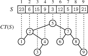
Figure 1: Illustration for Cartesian tree $\mathit{CT}(S)$ of $S=(\texttt{23},\texttt{6},\texttt{15},\texttt{9},\texttt{3},\texttt{12},\texttt{5},\texttt{19},\texttt{21})$. Since the minimum value among $S$ is $S[5]$, node $v=5$ is the root of $\mathit{CT}(S)$, $\mathit{CT}(S[1..4])$ is the left subtree of $v$, and $\mathit{CT}(S[6..9])$ is the right subtree of $v$. Then, $v.\mathrm{L}=2$, $v.\mathrm{R}=7$, $S_{v}=S[1..9]=S$, $S_{v.\mathrm{L}}=S[1..4]$, and $S_{v.\mathrm{R}}=S[6..9]$.

The Cartesian tree of string $S$, denoted by $\mathit{CT}(S)$, is the ordered binary tree recursively defined as follows: If $S=\varepsilon$, then $\mathit{CT}(S)$ is empty, and otherwise, $\mathit{CT}(S)$ is the tree rooted at $v$ such that the left subtree of $v$ is $CT(S[1..v-1])$, and the right subtree of $v$ is $CT(S[v+1..|S|])$, where $v=\mathsf{minidx}(S)$. For a node $v$, we denote by $v.\mathrm{L}$ the left child of $v$ if such a child exists and let $v.\mathrm{L}=\mathit{nil}$ otherwise. Similarly, we use the notation $v.\mathrm{R}$ for the right child of $v$. $CT(S)_{v}$ denotes the subtree of $CT(S)$ rooted at $v$. We say that two Cartesian trees $CT(S)$ and $CT(S^{\prime})$ are isomorphic as ordered trees [13], denoted $CT(S)=CT(S^{\prime})$.

There is an interplay between a sequence and its Cartesian tree as follows: We note that the indices of $S$ identify the nodes of $CT(S)$, and vice versa. For any node $v$ of $CT(S)$, we define the substring $S_{v}$ of $S$ recursively as follows:

1. If $v$ is the root of $CT(S)$, then $S_{v}=S=S[1..|S|]$.

2. If $v$ is a node with substring $S_{v}=S[\ell..r]$, then $S[v]$ is the minimum value in $S[\ell..r]$, $S_{v.\mathrm{L}}=S[\ell..v-1]$, and $S_{v.\mathrm{R}}=S[v+1..r]$.

An example of a Cartesian tree is shown in Figure 1.

2.3 Cartesian Tree Subsequence Matching

Let $T$ be a text string of length $n$ and $P$ be a pattern string of length $m\leq n$. We say that a pattern $P$ matches text $T$, denoted by $P\sqsubseteq T$, if there exists a subscript sequence $I=(i_{1},\ldots,i_{m})\in\mathcal{I}^{n}_{m}$ of $T$ such that $CT(T_{I})=CT(P)$ holds. Then, we refer to the subscript sequence $I$ as a trace.

A possible choice of the notion of occurrences of a pattern $P$ in $T$ is to employ the traces of $P$ as occurrences. However, it is not adequate since there can be exactly $\binom{n}{m}$ traces  for a text and a pattern of lengths $n$ and $m$. Instead, we employ minimal occurrence intervals as occurrences defined as follows.

Definition 1 (minimal occurrence interval).

For a text $T[1..n]$ and $P[1..m]$, an interval $[\ell,r]\subseteq[n]$ is said to be an occurrence interval for pattern $P$ over text $T$ if $P\sqsubseteq T[\ell..r]$ holds. It is said to be minimal if there is no occurrence interval $[\ell^{\prime},r^{\prime}]$ for $P$ over $T$ such that $[\ell^{\prime},r^{\prime}]\subsetneq[\ell,r]$.

Example 1.

Let text $T=(\mathtt{11},\mathtt{3},\mathtt{8},\mathtt{6},\mathtt{16},\mathtt{19},\mathtt{5},\mathtt{15},\mathtt{21},\mathtt{24})$ and pattern $P=(\mathtt{9},\mathtt{2},\mathtt{17},\mathtt{4},\mathtt{13})$. The occurrence interval $[3,9]$ for $P$ over $T$ is minimal since $I=(3,4,6,8,9)$ is a trace with $\mathit{CT}(T_{I})=\mathit{CT}(P)$, and there is no other occurrence interval $[\ell,r]\subsetneq[3,9]$ for $P$ over $T$. The interval $[1,8]$ is an occurrence interval, however, it is not minimal since there is another (minimal) occurrence interval $[1,5]\subsetneq[1,8]$ for $P$ over $T$. Overall, all minimal occurrence intervals for $P$ over $T$ are $[1,5]$ and $[3,9]$.

From the definition, there are $O(n^{2})$ occurrence intervals for $P$ over $T$, while there are $O(n)$ minimal occurrence intervals. If we have the set of all minimal occurrence intervals, we can easily enumerate all occurrence intervals in constant time per occurrence interval. Thus, we focus on minimal occurrences in this paper. Now, the main problem of this paper is formalized as follows:

Definition 2 (Cartesian Tree Subsequence Matching (CTMSeq)).

Given two strings $T[1..n]$ and $P[1..m]$, find all minimal occurrence intervals for $P$ over $T$.

We can easily see that CTMSeq can be solved in $O(m\binom{n}{m})$ time by simply enumerating all possible subscript sequences. However, its time complexities are too large to apply to real-world data sets. Hence, our goal here is to devise efficient algorithms running in polynomial time.

In the rest of this paper, we fix text $T$ of arbitrary length $n$ and pattern $P$ of arbitrary length $m$ with $0<m\leq n$.

3 $O(mn^{2})$-time Dynamic Programming Algorithm

This section describes an algorithm based on dynamic programming which runs in time $O(mn^{2})$. We later improve the running time to $O(mn\log\log n)$ in Section 4.

3.1 A Simple Algorithm

By dynamic programming approach, we can obtain a simple algorithm for CTMSeq with $O(mn^{3})$ time and $O(mn^{2})$ space complexities as follows. It recursively decides if the substring $P_{v}$ matches in $T[\ell..r]$ for all indices $v$ of $P$ and all intervals $[\ell..r]$ in $T$ from shorter to larger. These complexities mainly come from that it iterates the loop for $O(n^{2})$ possible intervals in $T$. In the following section, we devise more efficient algorithms in time and space complexities by introducing the notion of minimal fixed-intervals.

3.2 Minimal Fixed-interval

To solve CTMSeq without iterating for all possible intervals, we focus on fixing the corresponding locations between node $v$ of $CT(P)$ and index $i$ of $T$. For a node $v\in[m]$ and index $i\in[n]$, we refer to a pair $(v,i)$ as a $pivot$. Then, we define the minimal interval fixed with pivot $(v,i)$, called the minimal fixed-interval.

Definition 3 ((minimal) fixed-interval).

For pivot $(v,i)\in[m]\times[n]$, interval $[\ell,r]\subseteq[n]$ is called a fixed-interval with the pivot $(v,i)$ if there exists a trace $I=(i_{1},\ldots,i_{|P_{v}|})\in\mathcal{I}^{n}_{|P_{v}|}$ satisfying the following conditions (i)–(iv): (i) $i$ is an element of $I$, (ii) $[i_{1},i_{|P_{v}|}]\subseteq[\ell,r]$ (iii) $CT(T_{I})=CT(P_{v})$ holds, and (iv) $T[i]=\min(T_{I})$ holds. Furthermore, a fixed-interval $[\ell,r]$ with the pivot $(v,i)$ is said to be minimal if there is no fixed-interval $[\ell^{\prime},r^{\prime}]\subsetneq[\ell,r]$ with the pivot $(v,i)$

We show examples of (minimal) fixed-intervals on Figure 2.

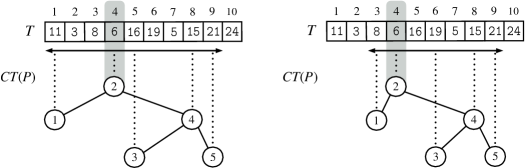
Figure 2: Illustration for fixed-intervals for the pivot $(v,i)$, where $T=(\mathtt{11}$, 3, 8, 6, 16, 19, 5, 15, 21, $\texttt{24})$, $P=(\mathtt{9}$, 2, 17, 4, $\texttt{13})$, and $(v,i)=(2,4)$. In the left figure, for the trace $I=(1,$ 4, $5$, $8$, $9)$ indicated by dotted lines, the interval $[1,9]$ is a fixed-interval with the pivot $(v,i)$. In the right figure, $[3,9]$ is a minimal fixed-interval with the pivot $(v,i)$ since there is no fixed-interval $[\ell,r]\subsetneq[3,9]$ with the pivot $(v,i)$.

Here, we give an essential lemma concerning minimal fixed-intervals.

Lemma 1.

For any pivot $(v,i)\in[m]\times[n]$, there exists at most one minimal fixed-interval with $(v,i)$.

Proof.

Assume that there are two minimal fixed-intervals with the pivot $(v,i)$. Let $[\ell,r]$ and $[\ell^{\prime},r^{\prime}]$ be two such distinct intervals. Without loss of generality, assume $\ell\leq\ell^{\prime}$. Then, by the minimalities of $[\ell,r]$ and $[\ell^{\prime},r^{\prime}]$, $\ell<\ell^{\prime}$ and $r<r^{\prime}$ must hold. From Definition 3, there exist $I=(\ell,\ldots,i,\ldots,r)$ and $I^{\prime}=(\ell^{\prime},\ldots,i,\ldots,r^{\prime})$ such that $\mathit{CT}(T_{I})=\mathit{CT}(T_{I^{\prime}})=\mathit{CT}(P_{v})$ and $T[i]=\min(T_{I})=\min(T_{I^{\prime}})$. Since $\mathit{CT}(T_{I})=\mathit{CT}(T_{I^{\prime}})$ and $T[i]=\min(T_{I})=\min(T_{I^{\prime}})$, the right subtree of $i$ in $\mathit{CT}(T_{I})$ is the same as that of $\mathit{CT}(T_{I^{\prime}})$. Namely, $\mathit{CT}(T_{I[i+1:r]})=\mathit{CT}(T_{I^{\prime}[i+1:r^{\prime}]})$ holds. Thus, we have $\mathit{CT}(T_{I^{\prime\prime}})=\mathit{CT}(P_{v})$ where $I^{\prime\prime}$ is the subscript sequence of length $|I|$ that is the concatenation of $I[\ell^{\prime}:i]$ and $I^{\prime}[i+1:r]$. Also, $i\in I^{\prime\prime}$ and $T[i]=\min(T_{I^{\prime\prime}})$ hold, and hence, $[\ell^{\prime},r]$ is a fixed-interval with the pivot $(v,i)$. This contradicts that $[\ell^{\prime},r^{\prime}]$ is a minimal fixed-interval. ∎

For convenience, we define the minimal fixed-interval with the pivot $(v,i)$ as $[-\infty,\infty]$ if there is no fixed-interval with the pivot $(v,i)$. We denote by $\mathsf{mfi}(v,i)$ the minimal fixed-interval with the pivot $(v,i)$. Let $\mathcal{M}=\{\mathsf{mfi}(\mathsf{minidx}(P),i)\mid i\in[n]\}$ be the set of all the minimal fixed-intervals for the root of $\mathit{CT}(P)$. By the definitions of minimal occurrence intervals and minimal fixed-intervals, the next corollary holds:

Corollary 1.

For any minimal occurrence interval $[\ell,r]$ for $P$ over $T$, $[\ell,r]\in\mathcal{M}$ holds. Contrary, for any interval $[\ell,r]\in\mathcal{M}$, if there is no interval $[\ell^{\prime},r^{\prime}]\subsetneq[\ell,r]$ such that $[\ell^{\prime},r^{\prime}]\in\mathcal{M}$, $[\ell,r]$ is a minimal occurrence interval for $P$ over $T$.

Note that not every intervals $[\ell,r]\in\mathcal{M}$ is a minimal occurrence interval for $P$ over $T$. We show an example of a interval $[\ell,r]\in\mathcal{M}$ such that $[\ell,r]$ is not a solution of CTMSeq in Figure 3.

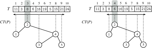
Figure 3: Illustration for two minimal fixed-intervals, where $T$ and $P$ are the same as in Figure 2. From the figure, $\mathsf{mfi}(2,3)=[1,9]$ and $\mathsf{mfi}(2,4)=[3,9]$ hold. Note that $\mathsf{mfi}(2,3)=[1,9]$ is not a solution of CTMSeq since $\mathsf{mfi}(2,4)\subsetneq\mathsf{mfi}(2,3)$ holds.

3.3 The Algorithm

From Corollary 1, once we compute the set $\mathcal{M}$ of intervals, we can obtain the solution of CTMSeq by removing non-minimal intervals from $\mathcal{M}$. Since every interval in $\mathcal{M}$ except $[-\infty,\infty]$ is a sub-interval of $[1,n]$, we can sort them in $O(n)$ time by using bucket sort, and thus, can also remove non-minimal intervals.

Thus, in what follows, we discuss how to efficiently compute $\mathcal{M}$, i.e., $\mathsf{mfi}(\mathsf{minidx}(P),i)$ for all $i\in[n]$. Now, we define two functions $L(v,i)=\ell$ and $R(v,i)=r$ for each node $v\in[m]$ in $\mathit{CT}(P)$ and each index $i\in[n]$, where $[\ell,r]=\mathsf{mfi}(v,i)$. Then, our task is, to compute $L(\mathsf{minidx}(P),i)$ and $R(\mathsf{minidx}(P),i)$ for all $i\in[n]$. Regarding the two functions, we show the following lemma (see also Figure 4 for illustration):

Lemma 2.

For any pivot $(v,i)\in[m]\times[n]$, the following recurrence relations hold:

$$L(v,i)=\left\{\begin{array}[]{ll}-\infty&\text{\rm{if}~{}}\mathsf{mfi}(v,i)=[-\infty,\infty],\\ i&\text{\rm{if}}\ \mathsf{mfi}(v,i)\neq[-\infty,\infty]\\ &\quad\text{\rm{and} }v.\mathrm{L}=\mathit{nil},\\ \displaystyle\max_{\begin{subarray}{c}1\leq j\leq i-1\end{subarray}}{\{L(v.\mathrm{L},j)\mid T[i]<T[j],R(v.\mathrm{L},j)<i\}}&\text{\rm{otherwise}}.\end{array}\right.$$

$$R(v,i)=\left\{\begin{array}[]{ll}\infty&\text{\rm{if}~{}}\mathsf{mfi}(v,i)=[-\infty,\infty],\\ i&\text{\rm{if}}\ \mathsf{mfi}(v,i)\neq[-\infty,\infty]\\ &\quad\text{\rm{and} }v.\mathrm{R}=\mathit{nil},\\ \displaystyle\min_{\begin{subarray}{c}i+1\leq j\leq n\end{subarray}}\{R(v.\mathrm{R},j)\mid T[i]<T[j],i<L(v.\mathrm{R},j)\}&\text{\rm{otherwise}}.\end{array}\right.$$

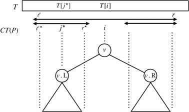
Figure 4: Illustration for intuitive understanding of recurrence relations in Lemma 2. The minimal fixed-interval $[\ell,r]$ with the pivot $(v,i)$ can be obtained from $\mathsf{mfi}(v.\mathrm{L},j)$ and $\mathsf{mfi}(v.\mathrm{R},k)$ by choosing $j$ and $k$ appropriately. As for the left subtree of $v$, the candidates for such $j$ must satisfy the conditions that the right-end of $\mathsf{mfi}(v.\mathrm{L},j)$ does not exceed $i-1$ and $T[j]>T[i]$. To minimize the width of fixed-intervals with $(v,i)$, we choose $j^{\star}$ that maximizes the left-end of $\mathsf{mfi}(v.\mathrm{L},j^{\star})$ while satisfying the above conditions. Also, symmetric arguments can be applied to the right subtree of $v$.

Proof.

We prove the validity of the first equation for $L(v,i)$. The second one can be proven by symmetric arguments. The first two cases are clearly correct by the definition of minimal fixed-intervals. We focus on the third case, when $\mathsf{mfi}(v,i)\neq[-\infty,\infty]$ and $v.\mathrm{L}\neq\mathit{nil}$.

Let $[\ell,r]=\mathsf{mfi}(v,i)$. By Definition 3, there exists $I=(\ell,\ldots,i,\ldots,r)$ such that $CT(T_{I})=CT(P_{v})$ and $T[i]=\min(T_{I})$. We notice that $\mathit{CT}(P_{v.\mathrm{L}})=\mathit{CT}(T_{I[\ell:\mathit{pre}_{i}]})$ holds where $\mathit{pre}_{i}$ is the subscript preceding $i$ in $I$. Thus, there exists $k$ such that $\ell\leq k\leq i-1$, $T[i]<T[k]$, $R(v.\mathrm{L},k)<i$, and $L(v.\mathrm{L},k)\geq\ell$. Now, let $j^{\star}:=\operatorname*{arg\,max}_{1\leq j\leq i-1}\{L(v.\mathrm{L},j)\mid T[i]<T[j],R(v.\mathrm{L},j)<i\}$ and $[\ell^{\star},r^{\star}]:=\mathsf{mfi}({v.\mathrm{L}},j^{\star})$. Then, $\ell^{\star}=L(v.\mathrm{L},j^{\star})\geq L(v.\mathrm{L},k)\geq\ell$ holds.

For the sake of contradiction, we assume $\ell<\ell^{\star}$. By Definition 3, there exists $I^{\star}=(\ell^{\star},\ldots,j^{\star},\ldots,r^{\star})$ such that $CT(T_{I^{\star}})=CT(P_{v.\mathrm{L}})$ and $T[j^{\star}]=\min(T_{I^{\star}})$. Also, by the definition of $j^{\star}$, $T[i]<T[j^{\star}]$ and $r^{\star}<i$ hold. Let $I^{\prime}$ be the concatenation of $I^{\star}$ and $I[i:r]$. Note that $I^{\prime}\in\mathcal{I}^{n}_{m}$ since $r^{\star}<i$. From the above discussions, $\mathit{CT}(T_{I^{\prime}})=\mathit{CT}(P_{v})$ holds since $\mathit{CT}(T_{I^{\star}})=\mathit{CT}(P_{v.\mathrm{L}})$ and $\min(T_{I^{\star}})=T[j^{\star}]>T[i]$. Also, $i\in I^{\prime}$ and $T[i]=\min(T_{I^{\prime}})$ clearly hold. Then, by Definition 3, $[\ell^{\star},r]\subsetneq[\ell,r]$ is a fixed-interval with $(v,i)$, however, this contradicts the minimality of $[\ell,r]=\mathsf{mfi}(v,i)$. Therefore, $\ell=\ell^{\star}$ holds. Namely, $L(v,i)=L(v.\mathrm{L},j^{\star})=\max_{1\leq j\leq i-1}\{L(v.\mathrm{L},j)\mid T[i]<T[j],R(v.\mathrm{L},j)<i\}$ holds. ∎

Algorithm 1 is a pseudo code of our algorithm to solve CTMSeq using dynamic programming based on Lemma 2.

Algorithm 1 Algorithm for solving CTMSeq using dynamic programming

1:procedure cartesian-tree-subsequence-match($T[1..n],P[1..m]$)

2:     $L[v][i]\leftarrow-\infty$ for all $v\in[m]$ and $i\in[n]$

3:     $R[v][i]\leftarrow\infty$ for all $v\in[m]$ and $i\in[n]$

4:     $C\leftarrow\mathit{CT}(P)$

5:     for each $v\in[m]$ in a bottom-up manner in $C$ do

6:         call UPDATE-LEFT-MAX($v,T,L,R$)

7:         call UPDATE-RIGHT-MIN($v,T,L,R$)      

8:     enumerate all minimal occurrence intervals for $P$ over $T$ by using $L$ and $R$.

9:function update-left-max($v,T,L,R$)

10:     if $v.\mathrm{L}=\mathit{nil}$ then

11:         $L[v][i]\leftarrow i$ for all $i\in[n]$

12:         return      

13:     for $i\leftarrow 1$ to $n$ do

14:         for $j\leftarrow 1$ to $i-1$ do

15:              if $T[i]<T[j]$ and $R[v.\mathrm{L}][j]<i$ then

16:                  $L[v][i]\leftarrow\displaystyle\max(L[v][i],L[v.\mathrm{L}][j])$                             

17:function update-right-min($v,T,L,R$)

18:     if $v.\mathrm{R}=\mathit{nil}$ then

19:         $R[v][i]\leftarrow i$ for all $i\in[n]$

20:         return      

21:     for $i\leftarrow 1$ to $n$ do

22:         for $j\leftarrow i+1$ to $n$ do

23:              if $T[i]<T[j]$ and $i<L[v.\mathrm{R}][j]$ then

24:                  $R[v][i]\leftarrow\displaystyle\min(R[v][i],R[v.\mathrm{R}][j])$                             

Correctness of Algorithm 1.

Algorithm 1 computes tables $L[v][i]=L(v,i)$ and $R[v][i]=R(v,i)$ for all pivot $(v,i)\in[m]\times[n]$ in a bottom-up manner in $\mathit{CT}(P)$ (see Line $5$). Since the recursion formulae of Lemma 2 hold for every node, Algorithm 1 correctly computes all the minimal fixed-intervals, and thus, all the minimal occurrence intervals for pattern $P$ over text $T$.

Time and Space Complexities of Algorithm 1.

At Line $4$, we build the Cartesian tree $C$ of a given pattern $P$. There is a linear-time algorithm to build a Cartesian tree [9], which takes $O(m)$ time here. In Lines 5–7, we call functions UPDATE-LEFT-MAX and UPDATE-RIGHT-MIN $m$ times since $C$ has $m$ nodes. It is clear that the functions UPDATE-LEFT-MAX and UPDATE-RIGHT-MIN run in $O(n^{2})$ time for each call. Thus, the total running time of Algorithm 1 is $O(mn^{2})$. Also, the space complexity of Algorithm 1 is $O(mn)$, which is dominated by the size of tables $L$ and $R$.

To summarize, we obtain the following theorem:

Theorem 1.

The CTMSeq problem can be solved in $O(mn^{2})$ time using $O(mn)$ space.

With a few modifications, we can reconstruct a trace $I=(\ell,\ldots,r)\in\mathcal{I}^{n}_{m}$ satisfying $CT(T_{I})=CT(P)$ for each minimal occurrence interval $[\ell,r]$. Precisely, when we compute the minimal fixed-interval with each pivot $(v,i)$, we simultaneously compute and store which index will correspond to the root of the left subtree of $v$ fixed at $i$. We do the same for the right subtree. Using the additional information, we can reconstruct a desired subscript sequence by tracing back from the root of $\mathit{CT}(P)$. The next corollary follows from the above discussion:

Corollary 2.

Once we compute $L(v,i)$ and $R(v,i)$ extended with the information of tracing back for all pivots $(v,i)\in[m]\times[n]$, we can find a trace $I=(\ell,\ldots,r)$ satisfying $CT(T_{I})=CT(P)$ for each minimal occurrence interval $[\ell,r]$ for $P$ over $T$ in $O(m)$ time using $O(mn)$ space.

4 Reducing Time to $O(mn\log\log n)$ with Predecessor Dictionaries

This section describes how to improve the time complexity of Algorithm 1 to $O(mn\log\log n)$. In Algorithm 1, functions UPDATE-LEFT-MAX and UPDATE-RIGHT-MIN require $O(n^{2})$ time for each call, which is a bottle-neck of Algorithm 1. By devising the update order of tables $L(v,i)$ and $R(v,i)$ and using a predecessor dictionary, we improve the running time of the above two functions to $O(n\log\log n)$.

4.1 Main Idea for Reducing Time

For any pivot $(v,i)\in[m]\times[n]$, let $\mathit{LFI}(v,i)=\{[L(v.\mathrm{L},j),R(v.\mathrm{L},j)]\mid 1\leq j\leq n,T[i]<T[j]\}$ be a set of intervals which are candidates for a component of the minimal fixed-interval with $(v,i)$. By Lemma 2, $L(v,i)=\max(\{\ell\mid[\ell,r]\in\mathit{LFI}(v,i),r<i\}\cup\{-\infty\})$ holds if $v.\mathrm{L}\neq\mathit{nil}$. Then, the next observations follow by the definitions:

• $\mathit{LFI}(v,i_{1})\subseteq\mathit{LFI}(v,i_{2})$ holds for any $i_{1},i_{2}$ with $T[i_{1}]>T[i_{2}]$.

• If there are intervals $[\ell_{1},r_{1}],[\ell_{2},r_{2}]\in\mathit{LFI}(v,i)$ such that $\ell_{2}=\ell_{1}\leq r_{1}<r_{2}$, then we can always choose $\ell_{1}$ as $L(v,i)$.

• If there are intervals $[\ell_{1},r_{1}],[\ell_{2},r_{2}]\in\mathit{LFI}(v,i)$ such that $\ell_{2}<\ell_{1}\leq r_{1}\leq r_{2}$, then $\ell_{2}$ is never chosen as $L(v,i)$.

The intuitive explanation of the third observation is shown in Figure 5.

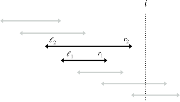
Figure 5: Illustration for the third observation for $\mathit{LFI}(v,i)$. The double-headed arrows represent the intervals in $\mathit{LFI}(v,i)$. The two intervals $[\ell_{1},r_{1}]$ and $[\ell_{2},r_{2}]$ are in $\mathit{LFI}(v,i)$ and $[\ell_{1},r_{1}]\subsetneq[\ell_{2},r_{2}]$ holds. It is clear that $\ell_{2}$ is never chosen as $L(v,i)$ for any $i\in[n]$.

From the third observation, we define a subset $\mathit{LFI}^{\prime}(v,i)$ of $\mathit{LFI}(v,i)$, whose conditions are sufficient to our purpose: Let $\mathit{LFI}^{\prime}(v,i)$ be the set of all intervals that are minimal within $\mathit{LFI}(v,i)$. Namely, $\mathit{LFI}^{\prime}(v,i)=\{[\ell,r]\in\mathit{LFI}(v,i)\mid$ there is no other interval $[\ell^{\prime},r^{\prime}]\in\mathit{LFI}(v,i)$ such that $[\ell^{\prime},r^{\prime}]\subsetneq[\ell,r]\}$. By the third observation,

$$L(v,i)=\max(\{\ell\mid[\ell,r]\in\mathit{LFI}^{\prime}(v,i),r<i\}\cup\{-\infty\})$$ (1)

holds if $v.\mathrm{L}\neq\mathit{nil}$.

The main idea of our algorithm is to maintain a set $\mathcal{S}_{v}$ of intervals so that it satisfies the invariant $\mathcal{S}_{v}=\mathit{LFI}^{\prime}(v,i)$. To maintain $\mathcal{S}_{v}$ efficiently, we utilize a data structure called predecessor dictionary for $\mathcal{S}_{v}$ supporting the following operations:

• $\texttt{insert}(\mathcal{S}_{v},\ell,r)$: insert interval $[\ell,r]$ into $\mathcal{S}_{v}$,

• $\texttt{delete}(\mathcal{S}_{v},\ell,r)$: delete interval $[\ell,r]$ from $\mathcal{S}_{v}$,

• $\texttt{pred}(\mathcal{S}_{v},x)$: return the interval $[\ell,r]\in\mathcal{S}_{v}$ on which $r$ is the largest among those satisfying $r<x$ (if it does not exist return $\mathit{nil}$), and

• $\texttt{succ}(\mathcal{S}_{v},x)$: return the interval $[\ell,r]\in\mathcal{S}_{v}$ on which $r$ is the smallest among those satisfying $x<r$ (if it does not exist return $\mathit{nil}$).

To implement a predecessor dictionary for $\mathcal{S}_{v}$, we use a famous data structure called van Emde Boas tree [22] that performs the operations as mentioned above in $O(\log\log n)$ time each. In general, the space usage of van Emde Boas tree is $O(U)$, where $U$ is the maximum of the integers to store. However, $U=n$ holds in our problem setting, and hence, the space complexity is $O(n)$.

4.2 Faster Algorithm

Algorithm 2 shows a function UPDATE-LEFT-MAX that computes $L(v,i)$ for all $i\in[n]$ based on the above idea. This function can be used to replace the function of the same name in Algorithm 1. The implementation of function UPDATE-RIGHT-MIN is symmetric.

Algorithm 2 Faster algorithm for UPDATE-LEFT-MAX using van Emde Boas tree

1:function UPDATE-LEFT-MAX($v,T,L,R$)

2:     if $v.\mathrm{L}=\mathit{nil}$ then

3:         $L[v][i]\leftarrow i$ for all $i\in[n]$

4:         return      

5:     $\mathcal{S}_{v}\leftarrow\emptyset$.

6:     for each $i\in[n]$ in the descending order of its value $T[i]$ do

7:         $[\ell,r]\leftarrow\texttt{pred}(\mathcal{S}_{v},i)$

8:         if $[\ell,r]=\mathit{nil}$ then

9:              $L[v][i]\leftarrow-\infty$

10:              continue          

11:         $L[v][i]\leftarrow\ell$

12:         $\ell_{\mathit{new}}\leftarrow L[v.\mathrm{L}][i]$, $r_{\mathit{new}}\leftarrow R[v.\mathrm{L}][i]$

13:         loop$\triangleright$ delete all intervals that become non-minimal

14:              $[\ell_{s},r_{s}]\leftarrow\texttt{succ}(\mathcal{S}_{v},r_{\mathit{new}}-1)$

15:              if $[\ell_{s},r_{s}]=nil$ or $[\ell_{\mathit{new}},r_{\mathit{new}}]\not\subseteq[\ell_{s},r_{s}]$ then

16:                  break               

17:              $\texttt{delete}(\mathcal{S}_{v},\ell_{s},r_{s})$          

18:         $[\ell_{p},r_{p}]\leftarrow\texttt{pred}(\mathcal{S}_{v},r_{\mathit{new}}+1)$

19:         if $[\ell_{p},r_{p}]=\mathit{nil}$ or $[\ell_{p},r_{p}]\not\subseteq[\ell_{\mathit{new}},r_{\mathit{new}}]$ then $\triangleright$ insert new interval if it is minimal

20:              $\texttt{insert}(\mathcal{S}_{v},\ell_{\mathit{new}},r_{\mathit{new}})$               

Correctness of Algorithm 2.

Remark that $v$ is fixed in Algorithm 2. Let $(i_{1},\ldots,i_{n})$ be the permutation of $[n]$ that is sorted in the order in which they are picked up by the for-loop at Line 6. We assume that the invariant $\mathcal{S}_{v}=\mathit{LFI}^{\prime}(v,i_{j})$ holds at the beginning of the $j$-th step of the for-loop. The value of $L[v][i_{j}]$ is determined at either Line 3, 9, or 11. By Lemma 2, $L[v][i_{j}]=L(v,i_{j})$ holds if the value determined at Line 3 or 9. By the invariant $\mathcal{S}_{v}=\mathit{LFI}^{\prime}(v,i_{j})$ and Equation 1, $L[v][i_{j}]=L(v,i_{j})$ also holds if the value determined at Line 11. Thus, $L(v,i_{j})$ is computed correctly.

Next, let us consider the invariant for $\mathcal{S}_{v}$. At Line 12, we set $[\ell_{\mathit{new}},r_{\mathit{new}}]$ the minimal fixed-interval with $(v.\mathrm{L},i_{j})$. In the internal loop at Lines 13–17, we delete all intervals $[\ell_{s},r_{s}]$ from $\mathcal{S}_{v}$ such that $[\ell_{s},r_{s}]$ becomes non-minimal within $\mathcal{S}_{v}\cup\{[\ell_{\mathit{new}},r_{\mathit{new}}]\}$. To do so, we repeatedly query $\texttt{succ}(\mathcal{S}_{v},r_{\mathit{new}}-1)$ and check whether the obtained interval includes $[\ell_{\mathit{new}},r_{\mathit{new}}]$. Finally, at the last two lines, we insert the new interval $[\ell_{\mathit{new}},r_{\mathit{new}}]$ if it does not include any other interval in $\mathcal{S}_{v}$. Then, any intervals in $\mathcal{S}_{v}$ are not nested each other, and thus, the invariant $\mathcal{S}_{v}=\mathit{LFI}^{\prime}(v,i_{j+1})$ holds at the end of the $j$-th step.

Time and Space Complexities of Algorithm 2.

We analyze the number of calls for each operation on a predecessor dictionary. Firstly, since insert is called only at Line $20$, it is called at most $n$ times throughout Algorithm 2. Similarly, pred at Line 7 and Line 18 is also called $O(n)$ times. From Line $13$ to Line $17$, succ and delete are called in the internal loop. The number of calls for delete is at most that of insert, and hence, delete is called at most $n$ times, and succ as well. Thus, throughout Algorithm 2, the total number of calls for all queries is $O(n)$. Therefore, the running time of Algorithm 2 is $O(n\log\log n)$. Also, the space complexity of Algorithm 2 is $O(n)$.

To summarize this section, we obtain the following lemma:

Lemma 3.

Algorithm 2 computes function UPDATE-LEFT-MAX in $O(n\log\log n)$ time using $O(n)$ space.

5 Reducing Space to $O(n\log m)$

This section describes how to reduce the space complexity of our algorithm to $O(n\log m)$. Having the tables $L[v][i]$ and $R[v][i]$ for all pivot $(v,i)\in[m]\times[n]$ requires $\Theta(mn)$ space. By Lemma 2, to compute the table values for node $v\in\mathit{CT}(P)$, we only need the table values for $v.\mathrm{L}$ and $v.\mathrm{R}$. Thus, we can discard the remaining values no longer referenced. However, even if we discard such unnecessary ones, the space complexity will not be improved in the worst case if we fix the order in which subtree is visited first: Let us assume that the left subtree is always visited first, and consider pattern

$$P=(k+1,1,\ldots,k+i,i,\ldots,2k,k,2k+1)$$ (2)

of length $m=2k+1$. It can be seen that every non-leaf node in $\mathit{CT}(P)$ has exactly two children, and the left child is a leaf (see also Figure 6 for a concrete example). Thus, when we process the node $v$ numbered with $2k$, we need to store at least $k+1$ tables since all tables for $k+1$ leaves have been created and not been discarded yet, and it yields $\Theta(mn)$ space.

Figure 6: Illustration for a worst case example of $CT(P)$ which causes the space complexity to be $\Theta(mn)$, where $P=(\mathtt{5},\mathtt{1},\mathtt{6},\mathtt{2},\mathtt{7},\mathtt{3},\mathtt{8},\mathtt{4},\mathtt{9})$. To compute the values of $L(v,i)$ and $R(v,i)$ for $v=8$, we only need the values of $L(u,i)$ and $R(u,i)$ for node $u\in\{7,9\}$. However, we have not finished computing $L(u,i)$ and $R(u,i)$ for node $u\in\{2,4,6\}$ yet, so we have to remember all of the values of $L(u,i)$ and $R(u,i)$ for node $u\in\{1,3,5,7,9\}$ simultaneously.

To avoid such a case, we add a new rule for which subtree is visited first; when we perform a depth-first traversal, we visit the larger subtree first if the current node $v$ has two children. Specifically, we visit the left subtree first if $|CT(P)_{v.\mathrm{L}}|>|CT(P)_{v.\mathrm{R}}|$, and visit the right subtree first otherwise, where the cardinality of a tree means the number of nodes in the tree. Clearly, the correctness of the modified algorithm relies on the original one (i.e., Algorithm 1) since the only difference is the rule that decides the order to visit.

In the following, we show that the rule makes the space complexity $O(n\log m)$. We utilize a technique called heavy-path decomposition [11] (a.k.a. heavy-light decomposition). For each internal node $v\in[m]$ in $\mathit{CT}(P)$, we choose one of $v$’s children with the larger subtree size and mark it as heavy, and we mark the other one as light if it exists. Exceptionally, we mark the root of $\mathit{CT}(P)$ as heavy. Then, it is known that the number of light nodes on any root-to-leaf path is $O(\log m)$ [11].

Now, we prove that the algorithm requires $O(n\log m)$ space at any step. Suppose we are now on node $u\in[m]$. Let $\mathsf{p}_{u}$ be the path from the root to $u$ in $\mathit{CT}(P)$. Note that each node $v$ on $\mathsf{p}_{u}$ is marked as either heavy or light. For each light node $v_{\ell}$ on $\mathsf{p}_{u}$, we have not discarded arrays $L$ and $R$ of size $O(n)$ associated with the sibling of $v_{\ell}$ to process the parent of $v_{\ell}$ in a later step. For each heavy node $v_{h}$ on $\mathsf{p}_{u}$, we do not have to remember any array since we recurse on $v_{h}$ first, and hence we require only $O(1)$ space for $v_{h}$. Since there are at most $O(\log m)$ light nodes on $\mathsf{p}_{u}$, the algorithm requires $O(n\log m)$ space at any step.

By combining these discussion with Theorem 1 and Lemma 3, we obtain our main theorem:

Theorem 2.

The CTMSeq problem can be solved in $O(mn\log\log n)$ time using $O(n\log m)$ space.

Note that the same method as for Corollary 2 can not be applied to the algorithm in this section since most tables are discarded to save space.

6 Preliminary Experiments

This section aims to investigate the behavior of each algorithm using artificial data. In the first experiment we use randomly generated strings to see how the algorithms would behave on average (Table 1). In the second experiment, we use the worst-case instance presented in Section 5 to check the worst-case behavior of the proposed algorithms (Table 2).

We conducted experiments on mac OS Mojava 10.14.6 with Intel(R) Core(TM) i5-7360U CPU @ 2.30GHz. For each test, we use a single thread and limit the maximum run time by 60 minutes. All programs are implemented using C++ language compiled with Apple LLVM version 10.0.1 (clang-1001.0.46.4) with -O3 optimization option. We compared the running time and memory usage of our four proposed algorithms below by varying the length $n$ of text and the length $m$ of pattern:

• basic: $O(mn^{2})$-time and $O(mn)$-space algorithm (Algorithm 1) explained in Section 3,

• basic-HL: $O(mn^{2})$-time and $O(n\log m)$-space algorithm obtained by applying the idea of memory reduction in Section 5 to basic.

• vEB: $O(mn\log\log n)$-time and $O(mn)$-space algorithm obtained by combining Algorithm 1 in Section 3 with Algorithm 2 in Section 4, and

• vEB-HL: $O(mn\log\log n)$-time and $O(n\log m)$-space algorithm obtained by applying the idea of memory reduction in Section 5 to vEB.

Tables 1 and 2 show the comparison of the performance among four algorithms above. NA indicates that the measurement was terminated when the execution time exceeded 60 minutes. Common to both Table 1 and Table 2, we use a text $T$ of length $n$ that is a randomly chosen permutation of $(1,2,\ldots,n)$, and thus, $T$ is a length-$n$ string over the alphabet $\{1,2,\ldots,n\}$. In Table 1, we use a pattern $P$ that is a randomly chosen subsequence of $T$, and thus, $P$ is also a length-$m$ string over the alphabet $\{1,2,\ldots,n\}$. In Table 2, we use the pattern $P=(k+1,1,\ldots,k+i,i,\ldots,2k,k)$ of length $m=2k$ in Equation 2 (see also Figure 6), which requires $\Theta(mn)$ space when the idea of memory reduction in Section 5 is not applied.

Table 1: Comparison of four algorithms for solving CTMSeq with randomly generated texts and patterns. The unit of time is second, and the unit of space is KB.

		basic		basic-HL		vEB		vEB-HL
$n$	$m$	time	space	time	space	time	space	time	space
$5000$	$50$	2.03	1980	0.09	3148	0.03	2496	0.03	2124
$5000$	$500$	19.20	2788	19.86	2168	0.37	3272	0.37	2596
$5000$	$1000$	40.62	2932	40.34	2236	0.73	3520	0.73	2604
$5000$	$2500$	96.27	3124	96.23	2368	1.84	3532	1.84	2816
$10000$	$50$	7.77	2128	7.74	1804	0.07	2504	0.07	2188
$10000$	$1000$	159.82	2740	159.70	1960	1.38	3128	1.38	2352
$10000$	$2000$	321.07	2920	323.09	2068	3.08	3312	3.09	2452
$10000$	$5000$	841.85	3252	835.29	2212	7.22	3644	7.23	2592
$50000$	$50$	206.49	4976	211.24	3836	0.39	6076	0.40	4920
$50000$	$5000$	NA	NA	NA	NA	39.98	13040	39.70	6576
$50000$	$10000$	NA	NA	NA	NA	79.42	12684	80.20	7044
$50000$	$25000$	NA	NA	NA	NA	199.14	13900	197.71	7340

Table 2: Comparison of four algorithms for solving CTMSeq with randomly generated texts and intentionally generated patterns of form $P=(k+1,1,\ldots,k+i,i,\ldots,2k,k)$ in Equation 2. The unit of time is second, and the unit of space is KB.

		basic		basic-HL		vEB		vEB-HL
$n$	$m$	time	space	time	space	time	space	time	space
$5000$	$50$	1.85	2572	1.86	1940	0.03	2920	0.03	2208
$5000$	$500$	18.01	11712	18.03	1912	0.23	12064	0.23	2372
$5000$	$1000$	37.65	21804	37.94	2028	0.41	22236	0.40	2516
$5000$	$2500$	92.58	52036	89.04	2220	0.96	52720	0.94	2960
$10000$	$50$	7.39	3444	7.45	1644	0.07	3748	0.07	2032
$10000$	$1000$	150.70	41632	153.18	1732	0.80	42192	0.79	2304
$10000$	$2000$	301.57	81856	303.77	1852	1.49	82584	1.46	2600
$10000$	$5000$	754.85	202408	759.71	2244	3.58	203656	3.49	3512
$50000$	$50$	186.05	12024	186.63	3048	0.37	13116	0.37	4140
$50000$	$5000$	NA	NA	NA	NA	18.36	650768	17.82	5616
$50000$	$10000$	NA	NA	NA	NA	35.42	963068	34.25	7112
$50000$	$25000$	NA	NA	NA	NA	87.28	998056	83.94	11600

Table 1 shows that the running time of vEB is faster than that of basic for all test cases, and the same result can be seen for vEB-HL and basic-HL. Comparing the memory usage of vEB with that of basic, it can be seen that the vEB uses more memory than basic, since the memory usage of the van Emde Boas tree is constant times larger than that of a basic array. The same is true for vEB-HL and basic-HL. The only difference between basic (vEB) and basic-HL (vEB-HL) is the search order of the tree traversal, so they have little difference in the running time for all test cases. Comparing these algorithms in terms of memory usage, it can be seen that the basic-HL (vEB-HL) uses less memory than basic (vEB), but the difference is not as pronounced as the theoretical difference in the space complexity. This is because $P$ is generated at random, so there is not much bias in the size of the subtrees.

On the other hand, the results in Table 2 show that basic-HL and vEB-HL are significantly more memory efficient than basic and vEB in the case where $m$ is large. This is consistent with the theoretical difference in the amount of the space complexity.

We also conducted the additional experiments with other algorithms:

• BST: $O(mn\log n)$-time and $O(mn)$-space algorithm using the binary search tree instead of van Emde Boas tree in Section 4, and

• BST-HL: $O(mn\log n)$-time and $O(mn)$-space algorithm obtained by applying the idea of memory reduction in Section 5 to BST.

vEB outperformed BST in both time and space for all test cases, and so do vEB-HL and BST-HL, which we feel is of independent interest. The details of the results are shown in Appendix A.

7 Conclusions

This paper introduced the Cartesian tree subsequence matching (CTMSeq) problem: Given a text $T$ of length $n$ and a pattern $P$ of length $m$, find every minimal substring $S$ of $T$ such that $S$ contains a subsequence $S^{\prime}$ which Cartesian-tree matches $P$. This is the Cartesian-tree version of the episode matching [7]. We first presented a basic dynamic programming algorithm running in $O(mn^{2})$ time, and then proposed a faster $O(mn\log\log n)$-time solution to the problem. We showed how these algorithms can be performed with $O(n\log m)$ space. Our experiments showed that our $O(mn\log\log n)$-time solution can be fast in practice.

An intriguing open problem is to show a non-trivial (conditional) lower bound for the CTMSeq problem. The episode matching (under the exact matching criterion) has $O((mn)^{1-\epsilon})$-time conditional lower bound under SETH [3]. Although a solution to the CTMSeq problem that is significantly faster than $O(mn)$ seems unlikely, we have not found such a (conditional) lower bound yet. We remark that the episode matching problem is not readily reducible to the CTMSeq problem, since CTMSeq allows for more relaxed pattern matching and the reported intervals can be shorter than those found by episode matching.

Acknowledgments

This work was supported by JSPS KAKENHI Grant Numbers JP20J11983 (TM), 20H00595 (HA), JST PRESTO Grant Number JPMJPR1922 (SI), and JST CREST Grant Number JPMJCR18K3 (HA).

The authors thank the anonymous referees for drawing our attention to reference [10].

Appendix A Additional Table

Table 3: Comparison of six algorithms with additional two algorithms for solving CTMSeq with randomly generated texts and patterns. The unit of time is second, and the unit of space is KB.

		basic		basic-HL		BST		BST-HL		vEB		vEB-HL
$n$	$m$	time	space	time	space	time	space	time	space	time	space	time	space
$5000$	$50$	2.03	1980	2.03	2020	0.09	3284	0.09	3148	0.03	2496	0.03	2124
$5000$	$500$	19.20	2788	19.86	2168	0.85	3896	0.83	3240	0.37	3272	0.37	2596
$5000$	$1000$	40.62	2932	40.34	2236	1.68	4084	1.67	3348	0.73	3520	0.73	2604
$5000$	$2500$	96.27	3124	96.23	2368	4.21	4396	4.18	3480	1.84	3532	1.84	2816
$10000$	$50$	7.77	2128	7.74	1804	0.20	4076	0.19	3360	0.07	2504	0.07	2188
$10000$	$1000$	159.82	2740	159.70	1960	3.70	4724	3.64	3940	1.38	3128	1.38	2352
$10000$	$2000$	321.07	2920	323.09	2068	8.25	4912	8.22	4048	3.08	3312	3.09	2452
$10000$	$5000$	841.85	3252	835.29	2212	20.25	5232	19.69	4196	7.22	3644	7.23	2592
$50000$	$50$	206.49	4976	211.24	3836	1.46	10204	1.45	10004	0.39	6076	0.40	4920
$50000$	$5000$	NA	NA	NA	NA	141.22	17276	136.76	10868	39.98	13040	39.70	6576
$50000$	$10000$	NA	NA	NA	NA	271.18	16920	272.29	11440	79.42	12684	80.20	7044
$50000$	$25000$	NA	NA	NA	NA	691.63	18144	689.80	11780	199.14	13900	197.71	7340

References

- [1] Brenda S. Baker. A theory of parameterized pattern matching: algorithms and applications. In S. Rao Kosaraju, David S. Johnson, and Alok Aggarwal, editors, Proceedings of the Twenty-Fifth Annual ACM Symposium on Theory of Computing, May 16-18, 1993, San Diego, CA, USA, pages 71–80. ACM, 1993. doi:10.1145/167088.167115.
- [2] Brenda S. Baker. Parameterized pattern matching: Algorithms and applications. J. Comput. Syst. Sci., 52(1):28–42, 1996. doi:10.1006/jcss.1996.0003.
- [3] Philip Bille, Inge Li Gørtz, Shay Mozes, Teresa Anna Steiner, and Oren Weimann. A conditional lower bound for episode matching. CoRR, abs/2108.08613, 2021.
- [4] Prosenjit Bose, Jonathan F. Buss, and Anna Lubiw. Pattern matching for permutations. Inf. Process. Lett., 65(5):277–283, 1998. doi:10.1016/S0020-0190(97)00209-3.
- [5] Sukhyeun Cho, Joong Chae Na, Kunsoo Park, and Jeong Seop Sim. A fast algorithm for order-preserving pattern matching. Inf. Process. Lett., 115(2):397–402, 2015. doi:10.1016/j.ipl.2014.10.018.
- [6] Maxime Crochemore, Costas S. Iliopoulos, Tomasz Kociumaka, Marcin Kubica, Alessio Langiu, Solon P. Pissis, Jakub Radoszewski, Wojciech Rytter, and Tomasz Walen. Order-preserving indexing. Theor. Comput. Sci., 638:122–135, 2016. doi:10.1016/j.tcs.2015.06.050.
- [7] Gautam Das, Rudolf Fleischer, Leszek Gasieniec, Dimitrios Gunopulos, and Juha Kärkkäinen. Episode matching. In Alberto Apostolico and Jotun Hein, editors, Combinatorial Pattern Matching, 8th Annual Symposium, CPM 97, Aarhus, Denmark, June 30 - July 2, 1997, Proceedings, volume 1264 of Lecture Notes in Computer Science, pages 12–27. Springer, 1997. doi:10.1007/3-540-63220-4\_46.
- [8] Noriki Fujisato, Yuto Nakashima, Shunsuke Inenaga, Hideo Bannai, and Masayuki Takeda. The parameterized suffix tray. In Tiziana Calamoneri and Federico Corò, editors, Algorithms and Complexity - 12th International Conference, CIAC 2021, Virtual Event, May 10-12, 2021, Proceedings, volume 12701 of Lecture Notes in Computer Science, pages 258–270. Springer, 2021. doi:10.1007/978-3-030-75242-2\_18.
- [9] Harold N. Gabow, Jon Louis Bentley, and Robert Endre Tarjan. Scaling and related techniques for geometry problems. In Richard A. DeMillo, editor, Proceedings of the 16th Annual ACM Symposium on Theory of Computing, April 30 - May 2, 1984, Washington, DC, USA, pages 135–143. ACM, 1984. doi:10.1145/800057.808675.
- [10] Pawel Gawrychowski, Samah Ghazawi, and Gad M. Landau. On indeterminate strings matching. In Proc. 31st Annual Symposium on Combinatorial Pattern Matching (CPM 2020), volume 161 of LIPIcs, pages 14:1–14:14, 2020.
- [11] Dov Harel and Robert Endre Tarjan. Fast algorithms for finding nearest common ancestors. SIAM J. Comput., 13(2):338–355, 1984. doi:10.1137/0213024.
- [12] Rui Henriques, Alexandre P. Francisco, Luís M. S. Russo, and Hideo Bannai. Order-preserving pattern matching indeterminate strings. In Annual Symposium on Combinatorial Pattern Matching (CPM 2018), volume 105 of LIPIcs, pages 2:1–2:15, 2018.
- [13] Christoph M. Hoffmann and Michael J. O’Donnell. Pattern matching in trees. J. ACM, 29(1):68–95, 1982. doi:10.1145/322290.322295.
- [14] Ramana M. Idury and Alejandro A. Schäffer. Multiple matching of parametrized patterns. Theor. Comput. Sci., 154(2):203–224, 1996. doi:10.1016/0304-3975(94)00270-3.
- [15] Orgad Keller, Tsvi Kopelowitz, and Moshe Lewenstein. On the longest common parameterized subsequence. Theor. Comput. Sci., 410(51):5347–5353, 2009. doi:10.1016/j.tcs.2009.09.011.
- [16] Jinil Kim, Peter Eades, Rudolf Fleischer, Seok-Hee Hong, Costas S. Iliopoulos, Kunsoo Park, Simon J. Puglisi, and Takeshi Tokuyama. Order-preserving matching. Theor. Comput. Sci., 525:68–79, 2014. doi:10.1016/j.tcs.2013.10.006.
- [17] Marcin Kubica, Tomasz Kulczynski, Jakub Radoszewski, Wojciech Rytter, and Tomasz Walen. A linear time algorithm for consecutive permutation pattern matching. Inf. Process. Lett., 113(12):430–433, 2013. doi:10.1016/j.ipl.2013.03.015.
- [18] Yoshiaki Matsuoka, Takahiro Aoki, Shunsuke Inenaga, Hideo Bannai, and Masayuki Takeda. Generalized pattern matching and periodicity under substring consistent equivalence relations. Theor. Comput. Sci., 656:225–233, 2016. doi:10.1016/j.tcs.2016.02.017.
- [19] Juan Mendivelso, Sharma V. Thankachan, and Yoan J. Pinzón. A brief history of parameterized matching problems. Discret. Appl. Math., 274:103–115, 2020. doi:10.1016/j.dam.2018.07.017.
- [20] Sung Gwan Park, Magsarjav Bataa, Amihood Amir, Gad M. Landau, and Kunsoo Park. Finding patterns and periods in Cartesian tree matching. Theor. Comput. Sci., 845:181–197, 2020. doi:10.1016/j.tcs.2020.09.014.
- [21] Siwoo Song, Geonmo Gu, Cheol Ryu, Simone Faro, Thierry Lecroq, and Kunsoo Park. Fast algorithms for single and multiple pattern Cartesian tree matching. Theor. Comput. Sci., 849:47–63, 2021. doi:10.1016/j.tcs.2020.10.009.
- [22] Peter van Emde Boas. Preserving order in a forest in less than logarithmic time and linear space. Inf. Process. Lett., 6(3):80–82, 1977. doi:10.1016/0020-0190(77)90031-X.