Prospects for extra Higgs boson search via $pp\to H,A\to\tau\mu,\tau\tau$
at the High Luminosity Large Hadron Collider

Abstract

We extend heavy Higgs searches at the Large Hadron Collider for $H\to\tau\mu$ by CMS, and $H\to\tau\tau$ by ATLAS and CMS, to study discovery prospects of extra Higgs states in $pp\to H,A\to\tau\mu,\tau\tau$ with $e\mu+\not{E}_{T}$ and $j_{\tau}\mu+\not{E}_{T}$ final states, where $j_{\tau}=\pi\,,\rho\,,a_{1}$ and $\not{E}_{T}$ is missing transverse energy. In a general two Higgs doublet model without $Z_{2}$ symmetry, extra Yukawa couplings $\rho_{\tau\tau}$ and $\rho_{\tau\mu}$ can drive $H,A\to\tau\tau$ and $\tau\mu$ channels at hadron colliders, following gluon-gluon fusion production with extra $\rho_{tt}$ couplings. The light Higgs boson $h(125)$ is found to resemble closely the Standard Model Higgs boson; in the alignment limit of $\cos\gamma\to 0$ for $h$–$H$ mixing, flavor changing neutral Higgs couplings such as $h\to\tau\mu$ are naturally suppressed, but the couplings of the heavier $H$ is optimized by $\sin\gamma\to 1$. We define various signal regions for $H,A\to\tau\mu$ and $\tau\tau$ and evaluate physics backgrounds from dominant processes with realistic acceptance cuts and tagging efficiencies. Two different studies are presented. We first perform a parton level study without any hadronization and with minimal detector smearing. We then include hadronization using PYTHIA 8.2 and fast detector simulation using DELPHES to give event level simulation. Results for $\sqrt{s}=13$ TeV appear promising, which we extend further to $\sqrt{s}=14$ TeV for the High Luminosity LHC.

I Introduction

A 125 GeV scalar, $h$, was discovered in 2012 by ATLAS and CMS ATLAS_SMHiggs ; CMS_SMHiggs , which resembles the Higgs boson of the Standard Model (SM), marking the success of SM up to the electroweak scale. Despite the remarkable resemblance of $h$ with the SM Higgs, we are still unclear about the nature of electroweak symmetry breaking (EWSB), and whether the SM Higgs sector is complete remains a mystery. Many extensions of SM expand the Higgs sector by adding additional doublets Branco:2011iw like two Higgs doublet models (2HDM), minimal SUSY (MSSM), three Higgs doublet model (3HDM) Keus:2013hya .

In this article, we study one of the simpler extensions of SM, a.k.a. 2HDM, where we extend the SM Higgs sector by an additional Higgs doublet, with both doublets coupling to fermions. As a result, we have two Yukawa matrices that cannot be simultaneously diagonalized, and thus we have off-diagonal flavor violating terms. The off-diagonal Yukawa terms can generate tree level flavor-changing neutral Higgs (FCNH) interactions; this version is referred to as 2HDM-III Hou:1991un or general 2HDM (g2HDM). The FCNH interactions are usually avoided by introducing some ad hoc $Z_{2}$ symmetries to enforce the Glashow-Weinberg natural flavor conservation (NFC) condition Glashow:1976nt , giving rise to 2HDM Type I, II, X, and Y versions Branco:2011iw . However, we do not enforce $Z_{2}$ symmetries but let nature provide us with its true flavor.

Recently, the Fermilab Muon g-2 experiment Muong-2:2021ojo confirmed the previous result of the BNL Muon g-2 experiment. Their combined result is,

$$a_{\mu}(\rm Exp)=116592061(41)\times 10^{-11}(0.35\,\rm ppm),$$ (1)

which deviates from the community consensus SM expectation Aoyama:2020ynm , $a_{\mu}(\rm SM)=116591810(43)\times 10^{-11}(0.37\,\rm ppm)$, by 4.2$\sigma$. The muon $g-2$ anomaly can be explained in g2HDM by flavor violating $\rho_{\tau\mu}$ couplings, as discussed in Refs. Wang:2021fkn ; Hou:2021sfl ; Athron:2021jyv . The lepton flavor violating (LFV) $\rho_{\tau\mu}$ and $\rho_{\mu\tau}$ couplings can drive $h\to\tau\mu$, which can be of concern as the limit CMS:htamu

$$\mathcal{B}(h\to\tau\mu)<0.15\,\%,$$ (2)

is rather stringent. However, one can overcome the strong bounds with the help of Alignment Hou:2017hiw . Under alignment the properties of $h$ closely resembles that of SM Higgs, which requires the mixing angle between the two CP-even scalars $h$, $H$ to approach zero, $\cos\gamma\to 0$, with the $h\tau\mu$ coupling $\propto\rho_{\tau\mu}\cos\gamma$.

In g2HDM, the exotic scalar $H$ benefit from alignment with $\sin\gamma\to 1$, and there is no suppression for $H\to\tau\mu$ or $A\to\tau\mu$ LFV processes. This property was exploited in Ref. Hou:2019grj ; Arganda:2019gnv , where a detailed collider search was performed. Subsequently, CMS published CMS:2019pex a detailed search for $H\to\tau\mu$ for $m_{H}\in[200,\,900]$ GeV with 35.9 fb^-1 data. No excess was found, placing strong limits on the $gg\to H\to\tau\mu$ cross section, but CMS has yet to update with full Run 2 data. The $\rho_{\tau\mu}$, $\rho_{\mu\tau}$ couplings along with $\rho_{tt}$ also contribute to $\tau\to\mu\gamma$ via two-loop Bjorken-Weinberg (or Barr-Zee) mechanism, which dominates over the one-loop mechanism, provided that $\rho_{tt}\sim\mathcal{O}(\lambda_{t})$ Chang:1993kw ; Hou:2020tgl . The one-loop effect would be suppressed if one takes Hou:2020itz $\rho_{\tau\tau}=\rho_{\tau\mu}=\rho_{\mu\tau}=\lambda_{\tau}\sim\mathcal{O}(0.01)$. We further extend our work from Ref. Hou:2019grj by respecting the current limits on $gg\to H\to\tau\mu$ cross-sections and $\mathcal{B}(\tau\to\mu\gamma)$.

The extra $\tau$ Yukawa coupling $\rho_{\tau\tau}$ with alignment is the main driver for the $gg\to H,A\to\tau\tau$ process. In addition, $\rho_{\tau\tau}$ can carry a complex phase, which can contribute to $\tau$ electric dipole moment Hou:2021zqq , or reveal itself in the CP structure of the $h\tau\tau$ coupling. The complex phase of the $h\tau\tau$ coupling is extensively searched by ATLAS ATLAS:2020evk and CMS CMS:2021sdq . In addition, CMS CMS:HTATA and ATLAS ATLAS:HTATA have also searched for the heavy exotic scalars decaying to $\tau\tau$ in the 200–2500 GeV mass range. This motivates us to study the collider prospects for $H,A\to\tau\tau$ and provide predictions for HL-LHC.

This article is organized as follows. We first briefly review g2HDM in Sec. II, and derive in Sec. III the constraints from the experiments on important couplings relevant to our collider study. Sec. IV discusses the prospects of $pp\to H,A\to\tau\mu+X$, while Sec. V is reserved for $pp\to H,A\to\tau\tau+X$. We present the discovery potential of both $\tau\mu$ and $\tau\tau$ in Sec. VI and conclude in Sec. VII.

II The general two Higgs doublet model

In g2HDM, one can write the Higgs potential in the Higgs basis, namely Hou:2017hiw ; Davidson:2005cw

$$V(\Phi,\Phi^{{}^{\prime}}) = \mu_{11}^{2}|\Phi|^{2}+\mu_{22}^{2}|\Phi^{\prime}|^{2}-(\mu_{12}^{2}\Phi^{\dagger}\Phi^{\prime}+h.c)+\frac{1}{2}\eta_{1}|\Phi|^{4}+\frac{1}{2}\eta_{2}|\Phi^{\prime}|^{4}$$ (3)

$$+ \eta_{3}|\Phi|^{2}|\Phi^{\prime}|^{2}+\eta_{4}|\Phi^{\dagger}\Phi^{\prime}|^{2}+\left[\Bigl{(}\frac{1}{2}\eta_{5}\Phi^{\dagger}\Phi^{\prime}+\eta_{6}|\Phi|^{2}+\eta_{7}|\Phi^{\prime}|^{2}\Bigr{)}\Phi^{\dagger}\Phi^{\prime}+h.c.\right],$$

where EWSB arises from $\Phi$ while $\langle\Phi^{\prime}\rangle=0$ (hence $\mu_{22}^{2}>0$). In Eq. (3), $\eta_{i}$s are the quartic couplings and taken as real, as we assume the Higgs potential is CP-invariant. After EWSB, one can find Hou:2017hiw from Eq. (3) the mass eigenstates $h$, $H$, $A$ and $H^{+}$, as well as $h$-$H$ mixing, where we define the mixing angle as $\gamma$. In the alignment limit, $\cos\gamma\to 0$.

The Yukawa couplings of the Higgs bosons to quarks are given as Davidson:2005cw ; Chen:2013qta ,

$$-\frac{1}{\sqrt{2}}\sum_{f=u,d} \bar{f}_{i}\left[(\lambda_{i}^{f}\delta_{ij}s_{\gamma}+\rho^{f}_{ij}c_{\gamma})h-(\lambda_{i}^{f}\delta_{ij}c_{\gamma}-\rho^{f}_{ij}s_{\gamma})H-i\,\mathrm{sgn}(\mathcal{Q}_{f})\rho^{f}_{ij}A\right]Rf_{j}$$ (4)

$$-\bar{u}_{i}\bigl{[}(V\rho^{d})_{ij}R-(\rho^{u\dagger}V)_{ij}L\bigr{]}d_{j}H^{+}+{\rm h.c.},$$

where $\lambda_{i}^{f}=\sqrt{2}m_{f}/v$ is the SM Yukawa coupling, $\rho^{f}$ is the extra Yukawa matrix and $c_{\gamma}(s_{\gamma})\equiv\cos\gamma(\sin\gamma)$. An analogous equation holds for charged leptons, but with $V$ set to unity because of the rather degenerate neutrinos. As discussed in the Introduction, $\rho^{f}$ can carry nonzero off-diagonal flavor violating terms. From Eq. (4), the extra Yukawa matrix $\rho^{f}$ is combined with $c_{\gamma}$ for $h$, hence the $hf\bar{f}$ coupling vanishes in the alignment limit of $c_{\gamma}\to 0$. As a result, all LFV processes such as $h\to\tau\mu$ as well as $t\to ch$ are highly suppressed in g2HDM. On the upside, $c_{\gamma}\to 0$ implies $s_{\gamma}\to 1$, and nonzero flavor violating couplings like $\rho_{tc}$,  $\rho_{\tau\mu}$ can drive our signal $gg\to H,A\to\tau\mu$ processes, or $gg\to H,A\to tc$ Altunkaynak:2015twa , even process like $cg\to tH,tA\to tt\bar{c}$ Kohda:2017fkn ; Gori:2017tvg , $cg\to tH,tA\to t\tau\mu$ and $cg\to bH^{+}\to bt\bar{b}$ Ghosh:2019exx , $bHW^{+}(\to b\tau\mu W^{+},btcW^{+}$ Hou:2021sfl ). We hence see that, even in the alignment limit, g2HDM can provide a rich phenomenology at the LHC.

The $\rho_{\tau\tau}$ coupling in the alignment limit is one of the drivers for our second signal process, $pp\to H,A\to\tau\tau$. In addition, with complex $\rho_{\tau\tau}$, the $h\tau\tau$ coupling can become complex hence CP violating, with the phase Hou:2021zqq ,

$${\tan\phi_{h\tau\tau}=\frac{c_{\gamma}\,{\rm Im}\,\rho_{\tau\tau}}{c_{\gamma}\,{\rm Re}\,\rho_{\tau\tau}+s_{\gamma}\,\lambda_{\tau}}.}$$ (5)

In this article, we do not explore the complexity of $\rho_{\tau\tau}$ and $\rho_{\tau\mu}$ but keep them real for simplicity. Furthermore, unlike Ref. Hou:2021sfl , we follow the “normal” or conservative guesstimate Hou:2020itz of the associated extra Yukawa couplings,

$$\rho_{\tau\tau}=\rho_{\tau\mu}=\mathcal{O}(\lambda_{\tau}),\quad\ \rho_{tt}=\mathcal{O}(\lambda_{t}).$$ (6)

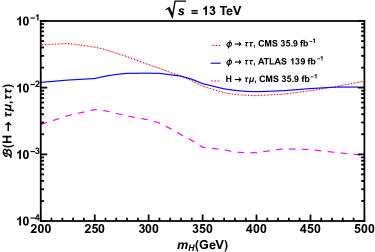
Figure 1: Limits from CMS and ATLAS on $\mathcal{B}(H\to\tau\mu,\tau\tau)$ under the assumption of SM-like (exotic) $H$ production.

III Constraints on relevant parameters

The important parameters governing $pp\to H,A\to\tau\mu+X$ and $pp\to H,A\to\tau\tau+X$ are $\rho_{\tau\mu}$, $\rho_{\tau\tau}$, $\rho_{tt}$, $c_{\gamma}$. Finite $\rho_{tc}$ can drive $H,A\to t\bar{c}+\bar{t}c$ Altunkaynak:2015twa and dilute $H,A\to\tau\mu,\tau\tau$. Note that $\rho_{ct}$ suffers strict constraints from $B_{s}$–$\bar{B}_{s}$ mixing as it enters the process via top-loop Crivellin:2013wna , while $\rho_{tc}c_{\gamma}$ is bound by direct searches by CMS and ATLAS for $t\to ch$ decay. Recently, CMS CMS:2021hug puts the most stringent bound on $\mathcal{B}(t\to ch)<7.3\times 10^{-4}$ at 95% C.L. with $h\to\gamma\gamma$ (this has been recently surpassed by ATLAS ATLAS:2023ujo , though at comparable sensitivity). Note that the bound depends on $c_{\gamma}$, and in the alignment limit ($c_{\gamma}\to 0$) the bound vanishes. An interesting point about the $t\to ch\to c\gamma\gamma$ channel is that both $\rho_{tc}$ through $tch$ and $\rho_{tt}$ via $h\gamma\gamma$ enters the decay chain. However, in this article we do not explore the implications of the CMS $t\to ch$ study on the interplay between $\rho_{tt}$ and $\rho_{tc}$ couplings, since both effects vanish with alignment. Following a simple scaling of Aaboud:2018oqm ; Jain:2019ebq ; Gutierrez:2020eby ,

$$\lambda_{tch}\equiv\rho_{tc}\rm c_{\gamma}=1.92\times\sqrt{\mathcal{B}(t\to ch)}.$$ (7)

we get $\rho_{tc}<$ 0.52 and 5.2 for $c_{\gamma}$ =0.1, and 0.01, respectively.

The $\rho_{tt}$ coupling is responsible for the production of the exotic scalars by gluon-gluon fusion via top-loop, and it is constrained by $B$ physics, especially $B_{q}$–$\bar{B}_{q}$ mixing and $b\to s\gamma$, as well as direct searches for $gg\to\bar{t}H^{+}b\to\bar{t}t\bar{b}b+{\rm h.c.}$ CMS:2020imj ; ATLAS:2021upq . We find that Hou:2019grj $B$ physics puts stronger bounds than direct searches. So we fix (Eq. (7) of Ref. Hou:2019grj )

$$\rho_{tt}=0.2\times\left(\frac{m_{H^{+}}}{150\;{\rm GeV}}\right)\,.$$ (8)

In Fig. 1 we present the limits on $\mathcal{B}(H\to\tau\mu)$ and $\mathcal{B}(H\to\tau\tau)$ assuming SM-Like production for simplicity. We do not enforce this assumption in the rest of the article. An interesting result emerges: we find that CMS $H\to\tau\mu$ is much more stringent than the ATLAS $H\to\tau\tau$. For the case of $pp\to H\to\tau\mu+X$, the exotic Higgs mass is reconstructed with the invariant mass, $M_{\tau\mu}$, using collinear approximation in tau decays that allows CMS to put a more stringent limit than $pp\to\phi\to\tau\tau+X$, in which they applied the less precise cluster transverse mass. For $pp\to H\to\tau\tau+X$ with 330 GeV $\lesssim m_{H}\lesssim$ 470 GeV, the CMS limit appears mildly better than ATLAS. However, it is probably within uncertainty.

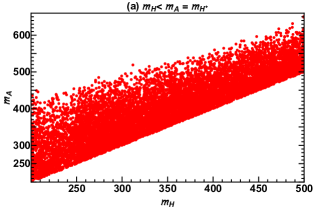
Figure 2: Scan of allowed points in $m_{A}$-$m_{H}$ plane for Cases A and B (see text for more details).

In this article, for simplicity we set all off-diagonal $\rho_{ij}=0$ except $\rho_{\tau\mu}$, and all diagonal $\rho_{ii}\sim\lambda_{i}$ except $\rho_{tt}$ and $\rho_{\tau\tau}$. The limits on the extra $\tau$ Yukawa couplings $\rho_{\tau\mu}$ and $\rho_{\tau\tau}$ depend on the choice of mass and mass differences for $A$, $H$ and $H^{+}$. We shall consider four different scenarios,

$${\rm Case\ A1}: \ m_{H}<m_{A}=m_{H^{+}},\;\rm c_{\gamma}=0.01,$$

$${\rm Case\ A2}: \ m_{H}<m_{A}=m_{H^{+}},\;\rm c_{\gamma}=0.1,$$

$${\rm Case\ B1}: \ m_{A}<m_{H}=m_{H^{+}},\;\rm c_{\gamma}=0.01,$$

$${\rm Case\ B2}: \ m_{A}<m_{H}=m_{H^{+}},\;\rm c_{\gamma}=0.1.$$ (9)

ATLAS ATLAS:2019nkf ; ATLAS:2021vrm and CMS CMS:2018uag have placed limits on $c_{\gamma}=\cos(\beta-\alpha)$ for 4 types of Yukawa interactions in two Higgs doublet models where extra Yukawa couplings are absent: Type I ($|c_{\gamma}|<0.3$), Types II, Lepton-Specific, and Flipped ($|c_{\gamma}|<0.1$). With extra Yukawa coupling matrices, however, it would be harder to constrain $c_{\gamma}$. But the fact that $h(125)$ so resembles the SM Higgs boson — alignment, for simplicity, we choose $c_{\gamma}=0.1$ and $0.01$ in Eq. (9) as benchmarks for the alignment limit.

We consider the mass difference $|m_{H}-m_{A}|=$ 150 GeV. A higher mass difference of around 150 GeV may run into various constraints. To show allowed parameter space, we perform a random scan by setting $m_{h}=125.1$ GeV, $\eta_{2}\in[0,5]$ and $\eta_{7}\in[-5,5]$, and for the lighter $H$ case scan $m_{H}\in[200,500]$ GeV and $m_{A}\in[200,700]$ GeV. The scan result is given in Fig. 2(a), and vice versa for the lighter $A$ case in Fig. 2(b). All the points in Fig. 2 satisfy (see e.g. Ref. Hou:2021sfl ) vacuum stability, perturbativity, unitarity and $T$-parameter constraints.

We see from Fig. 2 that the allowed $|m_{H}-m_{A}|$ difference decreases as we increase the mass of $H$ or $A$. We select $m_{H}=[200,500]$ GeV for Cases A1 and A2, and $m_{A}=[200,500]$ GeV for Cases B1 and B2, using some random points from scan that satisfy the mass-difference to get an estimate of $\lambda_{Hhh}$ Hou:2019qqi , i.e the trilinear-Higgs coupling for $H\to hh$. In Fig. 3 we present the branching fractions for different decay modes of $H$ and $A$ for all four cases of Eq. (9). Note that $\rm c_{\gamma}$ does not affect any fermionic decay width of $A$, although $\Gamma(A\to Zh)\propto|\rm c_{\gamma}|^{2}$.

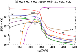
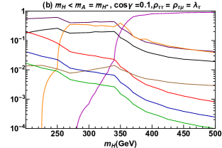
Figure 3: Branching fractions for (a), (b) $H$ decays, and (c), (d) $A$ decays.

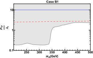
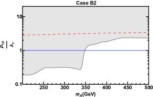
Figure 4: Limits on $\rho_{\tau\mu}$ from $H\to\tau\mu$ (gray-shaded), $h\to\tau\mu$ (blue-solid) and $\mathcal{B}(\tau\to\mu\gamma)$ (red-dashed).

Using the branching fractions from Fig. 3, we estimate the limits on $\rho_{\tau\mu}$ ($\rho_{\tau\mu}=\rho_{\mu\tau}$) from CMS, and find it to be more stringent than from Belle, where $\rho_{\tau\mu}$ and $\rho_{\mu\tau}$ also receive constraints from flavor physics, the most relevant one from $\tau\to\mu\gamma$. Belle recently measured Belle:2021ysv $\mathcal{B}(\tau\to\mu\gamma)<4.2\times 10^{-9}$ at 90 % C.L., improving slightly over the BaBar limit of $\mathcal{B}(\tau\to\mu\gamma)<4.4\times 10^{-9}$ BaBar:2009hkt at 90% C.L. The branching fraction of $\tau\to\mu\gamma$ is Omura:2015xcg ,

$$\mathcal{B}(\tau\to\mu\gamma)=\frac{48\pi^{3}\alpha}{G_{F}^{2}}(|A_{L}|^{2}+|A_{R}|^{2})\mathcal{B}(\tau\to\mu\nu_{\tau}\bar{\nu}_{\mu}),$$ (10)

where $\mathcal{B}(\tau\to\mu\nu_{\tau}\bar{\nu}_{\mu})=17.39\%$ ParticleDataGroup:2020ssz , and $A_{L(R)}$ are the amplitudes based on different chiral structures coming from one- and two-loop diagrams. We include one-loop effects from all $A$, $H$ and $H^{+}$, and likewise for Barr-Zee type two-loop contributions. Bounds on $\rho_{\tau\mu}$ from Belle is given in Fig. 4 red (dashed) for all four cases. We find the Belle bound from $\tau\to\mu\gamma$ is weaker than the CMS bound from $H\to\tau\mu$, and for all cases $\rho_{\tau\mu}$ can be lower than $\lambda_{\tau}$ below 2$m_{t}$ threshold; the bounds for lighter $A$ are even more stringent than lighter $H$ due to higher production cross section for the same values of mass. The $\mathcal{B}(\tau\to\mu\gamma)$ bounds show little mass dependence, largely because of our $\rho_{tt}$ from Eq. (8), increasing $\rho_{tt}$ compensates the suppression from heavier scalar mass of the two-loop diagram. We keep $\rho_{\tau\tau}=\lambda_{\tau}\sim 0.01$.

For $\rm c_{\gamma}\neq 0$, slightly away from the alignment limit, $pp\to h\to\tau\tau$ also puts constraints on $\rho_{\tau\tau}$ along with $pp\to H\to\tau\tau$ direct search by ATLAS and CMS. From Fig. 1, we select min(CMS, ATLAS) and use the $\rho_{tt}$ ansatz of Eq. (8) to estimate the bounds on $\rho_{\tau\tau}$ for the four cases of Eq. (9). Our results are presented in Fig. 5, where we keep $\rho_{\tau\mu}=\lambda_{\tau}$.

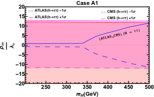
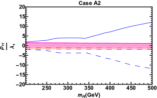
Figure 5: Limits on $\rho_{\tau\tau}$ from CMS CMS:2017zyp (salmon region) and ATLAS ATLAS:2018ynr (pink region) measurements of $\mathcal{B}(h\to\tau\tau)$ to within one standard deviation. Also shown are the bounds from CMS CMS:HTATA and ATLAS ATLAS:HTATA searches for $pp\to H\to\tau\tau+X$ (blue lines).

The $\rho_{\tau\mu}$ and $\rho_{\tau\tau}$ bounds are correlated, but since neither $\tau\mu$ nor $\tau\tau$ are the dominant decay mode, a closer look at the limits of Figs. 4 and 5, we find that they do not deviate much above $\mathcal{O}(\lambda_{\tau})$. We have checked that increasing one does not significantly affect the limits on the other from CMS and ATLAS searches. For $\tau\to\mu\gamma$, $\rho_{\tau\tau}$ only comes at one-loop level which is chiral-suppressed, hence Belle limits on $\rho_{\tau\mu}$ have no effect. We present the production cross sections for $pp\to H,A\to\tau\mu$ and $pp\to H,A\to\tau\tau$ in Figs. 6(a) and 6(b), respectively, using the $\rho_{tt}$ ansatz of Eq. (8) and branching fractions from Fig. 3.

IV Collider prospects for $H,A\to\tau\mu$

In this section we demonstrate our approach towards searching for the $H,A\to\tau\mu$ channel at LHC. For $\tau$ decay, we include $\tau\to e\nu_{e}\nu_{\tau}$ and $\tau\to j_{\tau}\nu_{\tau}$ decay modes, where $j_{\tau}=\pi,\rho,a_{1}$. We divide our collider study into two parts, (a) fully leptonic channel, $pp\to H,A\to\tau\mu\to e\mu+\not{E}_{T}+X$, and (b) semileptonic channel, $pp\to H,A\to\tau\mu\to j_{\tau}\mu+\not{E}_{T}+X$. We consider all four cases of Eq. (9). For simplicity we keep $\rho_{\tau\mu}=\rho_{\tau\tau}=\lambda_{\tau}$, but for estimating statistical significance, we follow the limits derived in previous section.

Analysis procedure and event generation. Two types of collider studies are performed: (a) parton level (PL) without hadronization or detector effects; (b) event level (EL) with hadronization using PYTHIA 8.2 pythia8 and detector effects simulated by DELPHES 3.5 delphes . For the parton level analysis, we use our code for phase-space integration using the VEGAS algorithm vegas . For the signal, we use analytic expressions from Kao:1993du to calculate $gg\to H,A$ production at tree level, then use HIGLU higlu to estimate higher-order corrections. We use CT14LO Dulat:2015mca parton distribution functions to calculate leading order (LO) processes.

For the backgrounds, we use MadGraph5 Alwall:2011uj and HELAS Hagiwara:2008jb libraries to extract matrix elements for all possible Feynman diagrams at LO and scale them using $K$-factors. We apply minimal smearing of lepton and jet momenta following ATLAS atlas_res and CMS CMS:2016lmd specifications. For simplicity, we keep the smearing for $e$ and $\mu$ the same:

$$\frac{\Delta E}{E}=\frac{0.6}{\sqrt{E(\rm GeV)}}\oplus 0.03\ (\rm jets),\quad\frac{\Delta E}{E}=\frac{0.25}{\sqrt{E(\rm GeV)}}\oplus 0.01\ (\rm leptons).$$ (11)

We use collinear approximation coll_app for $\tau$ decay at the parton level.

Figure 6: Production cross sections for (a) $pp\to H,A\to\tau\mu+X$, and (b) $\tau\tau+X$ for $\sqrt{s}$ = 13 TeV. The CMS2019 limits on $\tau\mu$ cross section and min(CMS,ATLAS) limits on $\tau\tau$ are also shown.

For the event level analysis, we first generate parton level events with Madgraph, then pass it to PYTHIA 8.2 and then DELPHES 3.5. We use the anti-$k_{T}$ algorithm antikt for jet clustering and keep all parameters at default values, as described in the DELPHES card for the CMS detector. The decays of $\tau$ leptons are modeled using TAUOLA Jadach:1990mz .

Fully leptonic channel and backgrounds. With $\tau\to e\nu_{e}\nu_{\tau}$, our signal is $pp\to H,A\to\tau\mu\to e\mu+\not{E}_{T}+X$. So in the final state we have two opposite sign, different flavor leptons along with missing transverse energy. Important backgrounds come from $W^{+}W^{-}$, $t\bar{t}$, $tW^{\pm}$ and $Z,\gamma^{*}\to\tau\tau$. We use TOP++ to estimate the $K$-factor for $t\bar{t}$ background toppp , and MCFM 8.0 mcfm to estimate the NLO corrections to remaining backgrounds. Since $\mu$ comes directly from Higgs decay, it is quite energetic, so we select events with $p_{T}(\mu)>$ 60 GeV and $|\eta(\mu)|<$ 2.4. For electron, we select events with $p_{T}(e)>$ 10 GeV, $|\eta(e)|<$ 2.4. In addition, we veto all events with extra jets and require $\not{E}_{T}>$ 20 GeV.

Variables	Leptonic	Semileptonic
$p_{T}(e)$	$>$ 10 GeV	NA
$p_{T}(\mu)$	$>$ 60 GeV	$>$ 60 GeV
$p_{T}(j_{\tau})$	NA	$>$ 30 GeV
$|\eta(e)|$	$<$ 2.4	NA
$|\eta(\mu)|$	$<$ 2.4	$<$ 2.4
$\not{E}_{T}$	$>$ 20 GeV	$>$ 20 GeV
$M_{T}(e,\not{E}_{T})$	$<$ 100 GeV	NA
$M_{T}(\mu,\not{E}_{T})$	$>$ 100 GeV	$>$ 100 GeV
$M_{T}(j_{\tau},\not{E}_{T})$	NA	$<$ 105 GeV
$|M_{\tau\mu}-m_{H}|$	$<0.2\,m_{H}$	$<0.2\,m_{H}$
$|\Delta\phi(e,\not{E}_{T})|$	$<$ 1.0	NA
$\Delta R(j_{\tau},\mu)$	NA	$>$ 0.4
$N_{j}$	NA	0 (PL)

Table 1: Cuts applied for leptonic and semileptonic channels in $H,A\to\tau\mu$ study.

For selected events, we reconstruct the transverse mass Barger:1987nn of a lepton ($\ell$) and missing transverse energy ($\not{E}_{T}$), $M_{T}(\ell,\not{E}_{T}),\ell=e$ or $\mu$, with

$$M^{2}_{T}(\ell,\not{E}_{T})=(p_{T}(\ell)+\not{E}_{T})^{2}-(\vec{p}_{T}(\ell)+\vec{\not{E}}_{T})^{2},$$ (12)

where $p_{T}(\ell)$ is the transverse momentum of electron or muon, while $M_{\tau\mu}$ is the reconstructed invariant mass of $\tau$ and $\mu$ with a pronounced peak near $m_{\phi},\phi=H$ or $A$, using collinear approximation Hagiwara:1989fn . In the collinear approximation, the $\tau$ coming from $H,A$ decay is highly boosted, hence we assume that its decay products are also boosted in the same direction. Under the collinear approximation, we can write,

$$p_{\rm vis}=x\,p_{\tau}\,,\quad{\rm and}\quad p_{\rm\nu}=(1-x)\,p_{\tau},$$ (13)

where $p_{vis}$ is the four-momentum of the visible particle(s) from $\tau$ decay, $p_{\rm\nu}$ is the total four momentum of all neutrinos from $\tau$ decay, and $x$ is the fraction of $\tau$ momentum carried by $p_{\rm vis}$. We know the four-momentum of the visible particles and $\not{E}_{T}$ coming from the $\nu$’s. After some algebra, we find

$$x=\frac{p_{T}(\rm vis)}{\sqrt{(p_{x}({\rm vis})+\not{E}_{x})^{2}+(p_{y}(\rm vis)+\not{E}_{y})^{2}}}\,.$$ (14)

Note that this assumption will only give reasonable results if the $\tau$ lepton is the only source of missing transverse energy, and that it is highly boosted. We select events that satisfy $M_{T}(e,\not{E}_{T})<$ 100 GeV and $M_{T}(\mu,\not{E}_{T})>$ 100 GeV CMS:2019pex .

Parton Level  ($pp\to H,A\to\tau\mu$)
Backgrounds/$m_{H}$	200 GeV	250 GeV	300 GeV	350 GeV	400 GeV	450 GeV	500 GeV
$W^{+}W^{-}$	9.73 fb	11.6 fb	11.0 fb	9.6 fb	7.8 fb	6.4 fb	5.1 fb
$Z,\gamma\to\tau\tau$	6.36 fb	4.2 fb	2.7 fb	1.8 fb	1.2 fb	0.8 fb	0.6 fb
$tW^{\pm}$	3.1 fb	4.2 fb	4.0 fb	3.7 fb	2.9 fb	2.4 fb	1.9 fb
$t\bar{t}$	3.1 fb	3.7 fb	3.3 fb	2.7 fb	2.3 fb	1.8 fb	1.4 fb
Total	22.3 fb	23.7 fb	21.1 fb	17.8 fb	14.5 fb	11.4 fb	9.0 fb
Event Level ($pp\to H,A\to\tau\mu$)
$W^{+}W^{-}$	4.87 fb	5.8 fb	5.4 fb	4.5 fb	3.4 fb	2.9 fb	2.5 fb
$Z,\gamma\to\tau\tau$	2.94 fb	1.9 fb	1.3 fb	0.7 fb	0.3 fb	0.2 fb	0.1 fb
$tW^{\pm}$	1.18 fb	1.7 fb	1.8 fb	1.5 fb	1.3 fb	1.0 fb	0.8 fb
$t\bar{t}$	0.83 fb	1    fb	0.9 fb	0.7 fb	0.6 fb	0.5 fb	0.4 fb
Total	9.82 fb	10.4 fb	9.3 fb	7.5 fb	5.9 fb	4.4 fb	3.7 fb

Table 2: Background cross sections for $e\mu$ final state at parton and event levels.

Figure 7: Cross sections after all cuts at parton (a, c), and event (b, d) levels for $pp\to H,A\to\tau\mu$. Upper (lower) panels are for the (semi-)leptonic channel.

We define a moving mass window of $|M_{\tau\mu}-m_{H,A}|<0.2\times m_{H,A}$ to estimate the irreducible background from SM processes for a particular $m_{H}$. All the cuts discussed here are summarized in Table 1. Cross sections of all backgrounds for PL and EL are presented in Table 2. The signal cross sections are given in Figs. 7(a) and (b). It is important to note that two b-veto plays a vital role in suppressing $t\bar{t}$ background. In the CMS CMS:2019pex study, their $t\bar{t}$ enriched control region requires at least 1-jet to be tagged as a b-jet. We have checked that when we select events that contain at least 1 b-jet the $t\bar{t}$ becomes the most dominant background almost 20 times the contribution from $W^{+}W^{-}$.

Semileptonic channel and backgrounds. When $\tau$ decays hadronically to $j_{\tau}$, the signal becomes $pp\to H,A\to\tau\mu\to j_{\tau}\mu+\not{E}_{T}+X$, giving us a final state with one jet tagged as a $\tau$-jet, one $\mu$ and missing transverse energy. Important backgrounds come from $W^{\pm}j$, $t\bar{t}$, $W^{+}W^{-}$, $Z,\gamma^{*}\to\tau\tau$ and $tW^{\pm}$. Event selection is similar to the leptonic channel. Following CMS CMS:2019pex , we require $p_{T}(j_{\tau})>$ 30 GeV and $|\eta(j_{\tau})|<2.5$, with muon selection the same as before. We again reconstruct the transverse masses $M_{T}(\mu,\not{E}_{T})$ and $M_{T}(j_{\tau},\not{E}_{T})$, then the collinear mass $M_{\tau\mu}$ using Eqs. (13) and (14) to reconstruct $\tau$ four momentum. Cuts on the reconstructed transverse masses are taken from CMS CMS:2019pex and summarized in Table 1. Background cross sections after all cuts in Table 1 are applied for different Higgs masses are given in Table 3. The signal cross sections as a function of Higgs mass are given in Figure 7(c) and 7(d). We scale the parton level signal cross section and $Z,\,\gamma^{*}\to\tau\tau$ with $\epsilon_{j_{\tau}}$ = 0.7 Friis:2011zz , and the mistag rates at 1/35 for 1-prong and 1/240 for 3-prong $\tau$ decays ATLAS:2019uhp .

Parton Level  ($pp\to H,A\to\tau\mu$)
Backgrounds/$m_{H}$	200 GeV	250 GeV	300 GeV	350 GeV	400 GeV	450 GeV	500 GeV
$W^{\pm}j$	210.42 fb	192.7 fb	143.9 fb	98.6 fb	66.4 fb	45.2 fb	31.3 fb
$t\bar{t}$	9.49 fb	13.5 fb	12.9 fb	10.4 fb	7.8 fb	5.6 fb	4.1 fb
$W^{+}W^{-}$	3.22 fb	3.5 fb	2.9 fb	2.2 fb	1.7 fb	1.2 fb	0.9 fb
$tW^{\pm}$	1.63 fb	2.2 fb	2.2 fb	1.9 fb	1.4 fb	1.1 fb	0.9 fb
$Z,\gamma\to\tau\tau$	4.14 fb	2.1 fb	2.0 fb	1.6 fb	1.2 fb	0.9 fb	0.7 fb
Total	228.9 fb	214.0 fb	163.9 fb	114.6 fb	78.5 fb	54.0 fb	37.8 fb

Table 3: Background cross sections for $j_{\tau}\mu$ final state after cuts at PL.

Variables	Leptonic	Semi-leptonic
$p_{T}(e)$	$>$ 13 GeV	NA.
$p_{T}(\mu)$	$>$ 10 GeV	$>$ 30 GeV
$p_{T}(j_{\tau})$	NA	$>$ 25 GeV
$|\eta(e)|$	$<$ 2.5	NA
$|\eta(\mu)|$	$<$ 2.4	$<$ 2.5
$|\eta(j_{\tau})|$	NA	$<$ 2.3
$\not{E}_{T}$	$>$ 20 GeV	$>$ 20 GeV
$M_{T}(\mu,\not{E}_{T})$	$<$ 50 GeV	$<$ 50 GeV
$M_{T}(e,\mu,\not{E}_{T})$	$(0.4\,m_{H},0.95\,m_{H})$	NA
$M_{T}(j_{\tau},\mu,E_{T})$	NA	$(0.4\,m_{H},0.95\,m_{H})$
$\Delta R(e,\mu)$	(3,4.5)	NA
$\Delta R(\tau_{j},\mu)$	NA	$>$ 2.4
$N_{j}$	NA	0

Table 4: Cuts for $H,A\to\tau\tau$.

V Collider prospects for $H,A\to\tau\tau$

The $H,A\to\tau\tau$ process is more challenging than $H,A\to\tau\mu$ to probe at LHC because mass reconstruction is poorer. The tau pairs from $gg\to H,A\to\tau\tau$ are back to back. It is difficult to determine the invariant mass of tau pairs ($M_{\tau\tau}$). Thus we rely on the transverse mass with visible particles and missing transverse energy from tau decays. Furthermore, for $\rho_{\tau\tau}=\rho_{\tau\mu}=\lambda_{\tau}$, the $H,A\to\tau\tau$ final state has half the event rate compared to $H,A\to\tau^{+}\mu^{-}+\tau^{-}\mu^{+}$. Although there is no flavor violation, we consider the same final state as $\tau\tau\to e\mu+\not{E}_{T},\ j_{\tau}\mu+\not{E}_{T}$.

Contribution of $\tau\mu$ in $\tau\tau$. With the same final state, obviously $H,A\to\tau\mu$ can contribute to $H,A\to\tau\tau$. However, we find that $M_{T}(\mu,\not{E}_{T})$ is a powerful variable in separating the $\tau\tau$ signal from $\tau\mu$. This is because $M_{T}(\mu,\not{E}_{T})>$ 100 GeV for $\tau\mu$, while $M_{T}(\mu,\not{E}_{T})<50$ GeV for $\tau\tau$, as $\mu$ from the former comes from Higgs decay whereas for $\tau\tau$ it comes from $\tau$ decay.

For $H,A\to\tau\tau$, both leptons (fully leptonic) and $j_{\tau}$ + lepton (semileptonic) come from $\tau$ decay, which give 4 and 3 neutrinos, respectively, in the final state. This makes the collinear approximation weaker for mass reconstruction. So we rely on cluster transverse mass of two visibly decaying $\tau$’s and $\not{E}_{T}$ ($M_{T}(\tau_{\rm vis1},\tau_{\rm vis2},\not{E}_{T})$), which is given as Barger:1987nn ,

$$M_{T}^{2}(\tau_{\rm vis1},\tau_{\rm vis2},\not{E}_{T})= \left(\sqrt{|\vec{p}_{T}(\tau_{\rm vis1},\tau_{\rm vis2})|^{2}+M^{2}(\tau_{\rm vis1},\tau_{\rm vis2})}+\not{E}_{T}\right)^{2}$$

$$\ \ \ -\left(\vec{p}_{T}(\tau_{\rm vis1},\tau_{\rm vis2})+\vec{\not{E}}_{T}\right)^{2},$$ (15)

with $M(\tau_{\rm vis1},\,\tau_{\rm vis2})$ and $\vec{p}_{T}(\tau_{\rm vis1},\,\tau_{\rm vis2})$ the invariant mass and net transverse momentum of the two visible $\tau$ decays, respectively.

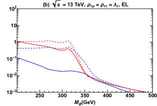
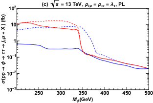
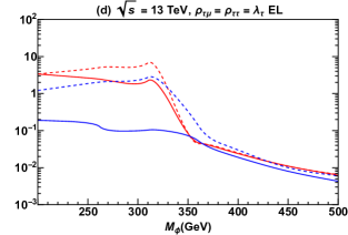
Figure 8: Cross sections for $pp\to H,A\to\tau\tau$ for both leptonic (a, b) and semileptonic (c, d) final states after applying all cuts at parton (a, c) and event (b, d) levels.

Following ATLAS ATLAS:HTATA , our selection rules for $e\mu$ and $j_{\tau}\mu$ final states are given in Table 4. The cross section for the signal at both EL and PL for leptonic and semileptonic channels is presented in Figure 8. The background cross sections are given in Table 5 after all cuts at both EL and PL for leptonic channel, and in Table 6 only at PL for semileptonic channel.

Parton Level ($pp\to H,A\to\tau\tau$)
Backgrounds/$m_{H}$	200 GeV	250 GeV	300 GeV	350 GeV	400 GeV	450 GeV	500 GeV
$Z,\gamma\to\tau\tau$	195.0 fb	38.6 fb	23.1 fb	15.3 fb	10.5 fb	7.6 fb	5.6 fb
$W^{+}W^{-}$	41.2 fb	52.5 fb	53.3 fb	48.3 fb	40.7 fb	32.9 fb	26.1 fb
$t\bar{t}$	3.60 fb	4.5 fb	4.8 fb	4.7 fb	4.3 fb	3.9 fb	3.4 fb
$tW^{\pm}$	2.66 fb	6.0 fb	6.6 fb	6.6 fb	6.2 fb	5.6 fb	5.0 fb
Total	243.5 fb	101.6 fb	87.8 fb	74.8 fb	61.8 fb	50 fb	40.0 fb
Event Level ($pp\to H,A\to\tau\tau$)
$Z,\gamma\to\tau\tau$	71.7 fb	14.2 fb	9.3 fb	6.6 fb	4.6 fb	3.4 fb	2.6 fb
$W^{+}W^{-}$	11.8 fb	15.0 fb	15.9 fb	14.9 fb	13.2 fb	11.1 fb	9.1 fb
$t\bar{t}$	1.9 fb	2.4 fb	2.8 fb	3.1 fb	3.1 fb	3.0 fb	2.7 fb
$tW^{\pm}$	0.9 fb	2.1 fb	2.6 fb	2.7 fb	2.6 fb	2.4 fb	2.1 fb
Total	86.3 fb	33.7 fb	30.5 fb	27.3 fb	23.4 fb	19.9 fb	16.5 fb

Table 5: Background cross sections for $e\mu$ final state after cuts at PL and EL in $\tau\tau$ channel.

Parton Level ($pp\to H,A\to\tau\tau$)
Backgrounds/$m_{H}$	200 GeV	250 GeV	300 GeV	350 GeV	400 GeV	450 GeV	500 GeV
$W^{\pm}j$	2790.9 fb	3463.7 fb	3515.4 fb	3215.5 fb	2794.3 fb	2365 fb	1976.1 fb
$Z,\gamma\to\tau\tau$	97.9 fb	118.7 fb	101.1 fb	81.2 fb	63.6 fb	49.6 fb	38.8 fb
$t\bar{t}$	44.8 fb	78.3 fb	99.9 fb	113.2 fb	112.2 fb	106.6 fb	96.3 fb
$tW^{\pm}$	8.1 fb	12.9 fb	16.6 fb	18.6 fb	19.2 fb	18.8 fb	17.6 fb
$W^{+}W^{-}$	6.6 fb	8.4 fb	8.7 fb	8.3 fb	7.6 fb	6.8 fb	6.1 fb
Total	2948.3 fb	3681.1 fb	3740.2 fb	3435.3 fb	2997.0 fb	2547.5 fb	2133.7 fb

Table 6: Background cross sections for $j_{\tau}\mu$ final state after cuts at PL in $\tau\tau$ channel.

VI Statistical Significance of the Signal

We now estimate the discovery potential of all channels we have discussed. We have kept $\rho_{\tau\mu}=\rho_{\tau\tau}=\lambda_{\tau}$ in Figs. 7 and 8 for simplicity. In this section, however, we consider the constraints on $\rho_{\tau\mu}$ and $\rho_{\tau\tau}$ as discussed in Figs. 4 and 5. We scale our signal cross section for $\tau\mu$ channel using the most strict limit for each case. For the $\tau\tau$ channel, especially with $h\to\tau\tau$ constraint coming into play, we use $\rho_{\tau\tau}<0$ limits to enhance the signal estimates for Cases A1 and A2, as $\lambda_{H\tau\tau}\simeq\lambda_{\tau}\rm c_{\gamma}-\rho_{\tau\tau}\rm s_{\gamma}$. For Cases B1 and B2, $A\to\tau\tau$ limits are more stringent for $m_{A}<2m_{t}$, and beyond which we choose the magenta dashed (CMS +1$\sigma$) of Fig. 5 to stay within experimental constraints.

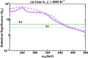
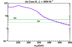
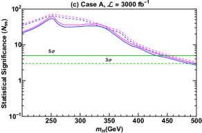
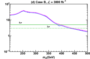
Figure 9: Statistical significance $N_{SS}$ for $pp\to H,A\to\tau\mu$ at PL, where (a), (b) are for the fully leptonic channel, and (c), (d) for the semileptonic channel. Both $\sqrt{s}$ = 13 (blue) and 14 TeV (magenta) are given, where solid (dashed) lines are for $\cos\gamma$ = 0.01 (0.1). The left panels (a, c) are for $m_{H}<m_{A}=m_{H^{+}}$, and (b, d) for $m_{A}<m_{H}=m_{H^{+}}$. We have used $\rho_{\tau\mu}=\rho_{\mu\tau}=$ limits, derived in Section III, i.e. Fig. 4.

To estimate significance, we assume Gaussian distribution, and denote $N_{S}$ as the number of signal events, and $N_{B}$ for background events (combining all background processes). The statistical significance $N_{SS}$ is evaluated with Cowan:2010js

$$N_{SS}=\sqrt{2(N_{B}+N_{S})\rm\ln(1+\frac{N_{S}}{N_{B}})-2N_{S}}\,.$$ (16)

For a large number of background events ($N_{B}\gg N_{S}$), it simplifies to become the well known discovery significance

$$N_{SS}=\frac{N_{S}}{\sqrt{N_{B}}}\,.$$ (17)

We estimate the statistical significance for each signal point using Eq. (16) at the parton level for $H,A\to\tau\mu$ and $H,A\to\tau\tau$, for both fully leptonic and semileptonic channels. We present our estimates for $N_{SS}$ at PL for $H,A\to\tau\mu$ and $H,A\to\tau\tau$, respectively, in Figs. 9 and 10 for $\sqrt{s}=$ 13 and 14 TeV at $\mathcal{L}=3\,\rm ab^{-1}$. In both figures, we give $N_{SS}$ for the purely leptonic channel in (a) and (b), and for semileptonic channels in (c) and (d).

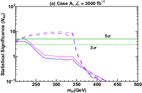
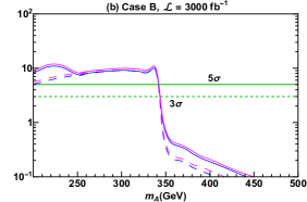
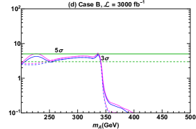
Figure 10: Same as Fig. 9 for $pp\to H,A\to\tau\tau$ at PL.

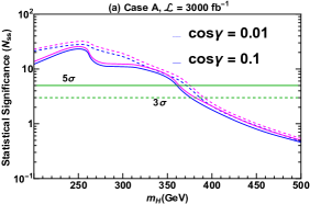
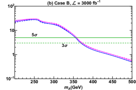
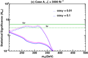
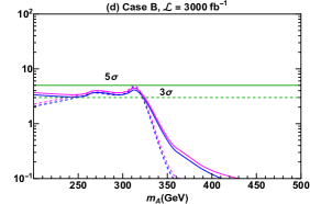
Figure 11: Statistical significance $N_{SS}$ at the event level for $pp\to H,A\to\tau\mu\to e\mu+\not{E}_{T}+X$ (top row) and $pp\to H,A\to\tau\tau\to emu+\not{E}_{T}+X$ (bottom row). Both $\sqrt{s}$ = 13 (blue) and 14 TeV (magenta) are presented, where solid (dashed) lines are for $\cos\gamma$ = 0.01 (0.1). The left panels (a, c) are for $m_{H}<m_{A}=m_{H^{+}}$, and (b, d) for $m_{A}<m_{H}=m_{H^{+}}$. We have chosen $\rho_{\tau\mu}=\rho_{\mu\tau}=$ limits, derived in Section III, i.e. Fig. 4.

We only present $N_{SS}$ for purely leptonic channel at EL for simplicity, which is given in Fig. 11 for $\tau\mu$ in (a) and (b), and for $\tau\tau$ in (c) and (d).

VII Discussion and Conclusion

Extra $\tau$ couplings $\rho_{\tau\tau}$ and $\rho_{\tau\mu}$ can act as good probes for exotic $H$, $A$ scalars below the $t\bar{t}$ threshold at HL-LHC. We have illustrated the prospects of discovering either $H$ or $A$ in $\tau\mu$ and $\tau\tau$ final states. We studied the constraint on relevant couplings from various searches and estimated the statistical significance at the HL-LHC with $3\,\rm ab^{-1}$ for $\sqrt{s}=13$, and 14 TeV.

From our study, we offer the following comments.

• CMS $H\to\tau\mu$ with $35.9\,\rm fb^{-1}$ data puts stronger bound on $\rho_{\tau\mu}$ than the latest Belle limit on $\tau\to\mu\gamma$, which is limited to the mass range considered in this study. Intuitively, if $H$ or $A$ approach $\mathcal{O}(\rm TeV)$, we expect Belle to do better. Limits from $h\to\tau\mu$ depends on $c_{\gamma}$, strengthening as $c_{\gamma}$ increases from 0.01 to 0.1.

• Constraints on $pp\to H\to\tau\tau$ from ATLAS and CMS follow an interesting trend: ATLAS is better for $m_{H}<330$ GeV, but after which CMS and ATLAS are comparable. This again tells the amazing sensitivity of CMS, as the data used is only a quarter that of ATLAS. Constraints from $pp\to h\to\tau\tau$ become important for $c_{\gamma}=0.1$.

• If $A$ is lighter, like in Cases B1 and B2, we find that the limits on $\rho_{\tau\mu}$ are the most stringent below $2m_{t}$, but becomes even weaker than Cases A1 and A2 ($H$ lighter) beyond $2m_{t}$. This is mainly due to $\Gamma(A\to t\bar{t})>\Gamma(H\to t\bar{t})$ with same mass. For all cases, the limits from CMS is better than $\rho_{\tau\mu}=\lambda_{\tau}$ at and below $2m_{t}$ threshold.

• From our PL study of $pp\to H,A\to\tau\mu$, we offer some insight:

  • Once we apply the $\rho_{\tau\mu}$ constraints, Cases B1 and B2 become almost identical.

  • For Cases A1 and A2, lower value of $c_{\gamma}$ does provide better significance, but above $2m_{t}$ they become pretty close to each other.

  • We see a slight bump for Case A2 around $2m_{t}$, which is again a reflection of the limits that we see in Fig. 4 as well as the rise in $pp\to H$ cross section at $t\bar{t}$ threshold.

  • We find that below 400 GeV, $H$ or $A$ can be discovered by HL-LHC with just a single channel. Above 400 GeV, significance can be improved by combining leptonic and semileptonic channels.

• The $pp\to H,A\to\tau\tau$ channel is much more challenging, owing to poor mass reconstruction for $pp\to H,A\to\tau\tau$ and lower branching fraction than $\tau\mu$ with $\rho_{\tau\tau}\simeq\rho_{\tau\mu}$. We draw the following remarks at the parton level:

  • Just like Cases B1 and B2 for $\tau\mu$, the statistical significance overlaps. We see an upward bump at the $t\bar{t}$ threshold, mainly due to the rise in production cross section. Beyond $2m_{t}$, the sharp rise of $t\bar{t}$ kills the $\tau\tau$ channel.

  • For Cases A1 and A2, $c_{\gamma}$ dependence is clearly visible, and we prefer lower $c_{\gamma}$ for better significance.

  • The semileptonic channel has a lower significance due to high QCD background compared to the much cleaner leptonic channel.

  • HL-LHC can still discover this channel up to $t\bar{t}$ threshold, beyond that, we need much smarter classification techniques.

  • Unlike $\tau\mu$ where we see less steep a fall in statistical significance, for $\tau\tau$ there is a sharp drop in significance after $2m_{t}$. This is mainly due to the limits on $\rho_{\tau\tau}$, which stay almost the same for nearly the entire mass range for all four cases.

• At the event level, the statistical significance follows a similar trend as PL for the $e\mu$ channel as discussed. However, we see a drop in significance due to detector resolution and hadronization effects. But we can still discover the $\tau\mu$ channel below $2m_{t}$, and hopefully, by combining with the semileptonic channel, the discovery range can be further extended. However, $\tau\tau$ remains challenging.

As discussed in Sec. III, we have set $\rho_{tc}=0$. A nonzero $\rho_{tc}$ can further dilute both signals. In Ref. Hou:2019grj , we showed that $\rho_{tc}\sim 0.5$ can dominate the branching fraction even beyond the $t\bar{t}$ threshold. However, we will need a very detailed study on overall impact of $\rho_{tc}\neq 0$, because it would relax the constraints from $H\to\tau\mu$ on $\rho_{\tau\mu}$ and from $H,A\to\tau\tau$ on $\rho_{\tau\tau}$. As discussed in Ref. Hou:2021xiq , for the mass range considered here, $\rho_{tc}\sim 0.5$ might be too high and a more reasonable value would be $\rho_{tc}\sim 0.1$. But in that study, all $\rho_{ij}$s except $\rho_{tc}$ are set to zero, and $c_{\gamma}=0$ was taken.

Another big motivation to study $\rho_{\tau\tau}$ and $\rho_{\tau\mu}$ is driven by electroweak baryogenesis (EWBG). As discussed in Ref. Guo:2016ixx ; Ge:2020mcl , complex extra $\tau$ couplings can also drive EWBG and explain matter-antimatter asymmetry of the Universe, although it has been questioned Cline:2021dkf whether light fermions can actually achieve this. The $h,H,A\to\tau\tau$ processes are also considered as good channels to study CP violation CMS:2021sdq ; Antusch:2020ngh , a necessary condition for EWBG. On the other side, there is EWBG driven by $\rho_{tt}$ and $\rho_{tc}$ Fuyuto:2017ewj , but it is unclear which way to go. Nonzero $\rho_{tc}$ and $\rho_{\tau\mu}$ opens up some exciting new channels, such as $cg\to tH,tA\to t\tau\mu$, $cg\to bH^{+}\to bHW^{+}\to bW^{+}\tau\mu$ Hou:2019grj , hence providing a rich phenomenology for LHC.

In this article, we find that beyond $2m_{t}$ it is quite challenging to probe either $H,A\to\tau\mu$ or $H,A\to\tau\tau$. However, we have to keep in mind that we have not considered all $\tau$-lepton decay modes, so by combining all channels of $\tau$ decay and performing more sophisticated machine learning classifications, the combined channels may hold promising future for discovering $H$ and $A$ at the HL-LHC, or even future FCC-hh or SppC colliders.

Although we have not focused on the case in this article, let us end with a positive note by connecting $pp\to H,\,A\to\tau\mu$ search with the recent confirmation of the muon $g-2$ anomaly. In g2HDM, the muon $g-2$ anomaly can be accounted for by sizable $\rho_{\tau\mu}\rho_{\mu\tau}$ and relatively low mass $H$ or $A$. If one takes the muon $g-2$ anomaly seriously, it may well mean that CMS $pp\to H,\,A\to\tau\mu$ search might draw a hint of a signal below the $2m_{t}$ threshold with full Run 2 data.

Acknowledgements: WSH and RJ are supported by MOST 110-2639-M-002-002-ASP of Taiwan, with WSH in addition by NTU 111L104019 and 111L894801. CK is supported by the University of Oklahoma.

References

- (1) G. Aad et al. [ATLAS], Phys. Lett. B 716, 1 (2012) [arXiv:1207.7214 [hep-ex]].
- (2) S. Chatrchyan et al. [CMS], Phys. Lett. B 716, 30 (2012) [arXiv:1207.7235 [hep-ex]].
- (3) G.C. Branco, P.M. Ferreira, L. Lavoura, M.N. Rebelo, M. Sher and J.P. Silva, Phys. Rept. 516, 1 (2012) [arXiv:1106.0034 [hep-ph]].
- (4) V. Keus, S.F. King and S. Moretti, JHEP 01, 052 (2014) [arXiv:1310.8253 [hep-ph]].
- (5) W.-S. Hou, Phys. Lett. B 296, 179 (1992).
- (6) S.L. Glashow and S. Weinberg, Phys. Rev. D 15, 1958 (1977).
- (7) B. Abi et al. [Muon g-2], Phys. Rev. Lett. 126, 141801 (2021) [arXiv:2104.03281 [hep-ex]].
- (8) T. Aoyama, N. Asmussen, M. Benayoun, J. Bijnens, T. Blum, M. Bruno et al., Phys. Rept. 887, 1 (2020) [arXiv:2006.04822 [hep-ph]].
- (9) H.-X. Wang, L. Wang and Y. Zhang, Eur. Phys. J. C 81, 1007 (2021) [arXiv:2104.03242 [hep-ph]].
- (10) W.-S. Hou, R. Jain, C. Kao, G. Kumar and T. Modak, Phys. Rev. D 104, 075036 (2021) [arXiv:2105.11315 [hep-ph]].
- (11) P. Athron, C. Balazs, T.E. Gonzalo, D. Jacob, F. Mahmoudi and C. Sierra, JHEP 01, 037 (2022) [arXiv:2111.10464 [hep-ph]].
- (12) A.M. Sirunyan et al. [CMS], Phys. Rev. D 104, 032013 (2021) [arXiv:2105.03007 [hep-ex]].
- (13) W.-S. Hou and M. Kikuchi, EPL 123, 11001 (2018) [arXiv:1706.07694 [hep-ph]].
- (14) W.-S. Hou, R. Jain, C. Kao, M. Kohda, B. McCoy and A. Soni, Phys. Lett. B 795, 371 (2019) [arXiv:1901.10498 [hep-ph]].
- (15) E. Arganda, X. Marcano, N. I. Mileo, R.A. Morales and A. Szynkman, Eur. Phys. J. C 79 (2019), 738 [arXiv:1906.08282 [hep-ph]].
- (16) A.M. Sirunyan et al. [CMS], JHEP 03, 103 (2020) [arXiv:1911.10267 [hep-ex]].
- (17) D. Chang, W.-S. Hou and W.-Y. Keung, Phys. Rev. D 48, 217 (1993) [arXiv:hep-ph/9302267 [hep-ph]].
- (18) W.-S. Hou and G. Kumar, Phys. Rev. D 101, 095017 (2020) [arXiv:2003.03827 [hep-ph]].
- (19) W.-S. Hou and G. Kumar, Phys. Rev. D 102, 115017 (2020) [arXiv:2008.08469 [hep-ph]].
- (20) W.-S. Hou, G. Kumar and S. Teunissen, [arXiv:2109.08936 [hep-ph]].
- (21) G. Aad et al. [ATLAS], Phys. Lett. B 805, 135426 (2020) [arXiv:2002.05315 [hep-ex]].
- (22) A. Tumasyan et al. [CMS], arXiv:2110.04836 [hep-ex].
- (23) A.M. Sirunyan et al. [CMS], JHEP 09, 007 (2018) [arXiv:1803.06553 [hep-ex]].
- (24) G. Aad et al. [ATLAS], Phys. Rev. Lett. 125, 051801 (2020) [arXiv:2002.12223 [hep-ex]].
- (25) S. Davidson and H.E. Haber, Phys. Rev. D 72, 035004 (2005) [erratum: Phys. Rev. D 72, 099902 (2005)] [arXiv:hep-ph/0504050 [hep-ph]].
- (26) K.-F. Chen, W.-S. Hou, C. Kao and M. Kohda, Phys. Lett. B 725, 378 (2013) [arXiv:1304.8037 [hep-ph]].
- (27) B. Altunkaynak, W.-S. Hou, C. Kao, M. Kohda and B. McCoy, Phys. Lett. B 751, 135 (2015) [arXiv:1506.00651 [hep-ph]].
- (28) M. Kohda, T. Modak and W.-S. Hou, Phys. Lett. B 776, 379 (2018) [arXiv:1710.07260 [hep-ph]].
- (29) S. Gori, C. Grojean, A. Juste and A. Paul, JHEP 01, 108 (2018) [arXiv:1710.03752 [hep-ph]].
- (30) D.K. Ghosh, W.-S. Hou and T. Modak, Phys. Rev. Lett. 125, 221801 (2020) [arXiv:1912.10613 [hep-ph]].
- (31) A. Crivellin, A. Kokulu and C. Greub, Phys. Rev. D 87, 094031 (2013) [arXiv:1303.5877 [hep-ph]].
- (32) A. Tumasyan et al. [CMS], Phys. Rev. Lett. 129, 032001 (2022) [arXiv:2111.02219 [hep-ex]].
- (33) G. Aad et al. [ATLAS], [arXiv:2309.12817 [hep-ex]].
- (34) M. Aaboud et al. [ATLAS], JHEP 05, 123 (2019) [arXiv:1812.11568 [hep-ex]].
- (35) R. Jain and C. Kao, Phys. Rev. D 99 (2019), 055036 [arXiv:1901.00157 [hep-ph]].
- (36) P. Gutierrez, R. Jain and C. Kao, Phys. Rev. D 103 (2021), 115020 [arXiv:2012.09209 [hep-ph]].
- (37) A.M. Sirunyan et al. [CMS], JHEP 07, 126 (2020) [arXiv:2001.07763 [hep-ex]].
- (38) G. Aad et al. [ATLAS], JHEP 06, 145 (2021) [arXiv:2102.10076 [hep-ex]].
- (39) G. Aad et al. [ATLAS], Phys. Rev. D 101 (2020) 012002 [arXiv:1909.02845 [hep-ex]].
- (40) [ATLAS], ATLAS-CONF-2021-053.
- (41) A.M. Sirunyan et al. [CMS], Eur. Phys. J. C 79 (2019) 421 [arXiv:1809.10733 [hep-ex]].
- (42) W.-S. Hou, M. Kohda and T. Modak, Phys. Rev. D 99, 055046 (2019) [arXiv:1901.00105 [hep-ph]].
- (43) A. Abdesselam et al. [Belle], JHEP 10, 19 (2021) [arXiv:2103.12994 [hep-ex]].
- (44) B. Aubert et al. [BaBar], Phys. Rev. Lett. 104, 021802 (2010) [arXiv:0908.2381 [hep-ex]].
- (45) Y. Omura, E. Senaha and K. Tobe, Phys. Rev. D 94, 055019 (2016) [arXiv:1511.08880 [hep-ph]].
- (46) P.A. Zyla et al. [Particle Data Group], PTEP 2020, 083C01 (2020).
- (47) T. Sjöstrand et al. Comput. Phys. Commun. 191, 159 (2015) [arXiv:1410.3012 [hep-ph]].
- (48) J. de Favereau et al. [DELPHES 3], JHEP 02, 057 (2014) [arXiv:1307.6346 [hep-ex]].
- (49) G.P. Lepage, J. Comput. Phys. 27, 192 (1978).
- (50) C. Kao, Phys. Lett. B 328, 420 (1994) [arXiv:hep-ph/9310206 [hep-ph]].
- (51) M. Spira, arXiv:hep-ph/9510347 [hep-ph].
- (52) S. Dulat et al. Phys. Rev. D 93, 033006 (2016) [arXiv:1506.07443 [hep-ph]].
- (53) J. Alwall, M. Herquet, F. Maltoni, O. Mattelaer and T. Stelzer, JHEP 06, 128 (2011) [arXiv:1106.0522 [hep-ph]].
- (54) K. Hagiwara, J. Kanzaki, Q. Li and K. Mawatari, Eur. Phys. J. C 56, 435 (2008) [arXiv:0805.2554 [hep-ph]].
- (55) [ATLAS], ATLAS-PHYS-PUB-2013-004.
- (56) V. Khachatryan et al. [CMS], JINST 12, P02014 (2017) [arXiv:1607.03663 [hep-ex]].
- (57) A.M. Sirunyan et al. [CMS], Phys. Lett. B 779 (2018), 283 [arXiv:1708.00373 [hep-ex]].
- (58) M. Aaboud et al. [ATLAS], Phys. Rev. D 99 (2019), 072001 [arXiv:1811.08856 [hep-ex]].
- (59) R.K. Ellis, I. Hinchliffe, M. Soldate and J.J. Van der Bij, Nucl. Phys. B 297, 221 (1988).
- (60) M. Cacciari, G.P. Salam and G. Soyez, JHEP 04, 063 (2008) [arXiv:0802.1189 [hep-ph]].
- (61) S. Jadach, J.H. Kühn and Z. Wa̧s, Comput. Phys. Commun. 64, 275-299 (1990).
- (62) M. Czakon and A. Mitov, Comput. Phys. Commun. 185, 2930 (2014) [arXiv:1112.5675 [hep-ph]].
- (63) R. Boughezal, J.M. Campbell, R.K. Ellis, C. Focke, W. Giele, X. Liu, F. Petriello and C. Williams, Eur. Phys. J. C 77, 7 (2017) [arXiv:1605.08011 [hep-ph]].
- (64) V.D. Barger and R.J.N. Phillips, Collider Physics (1987), ISBN 978-0-201-14945-6.
- (65) K. Hagiwara, A.D. Martin and D. Zeppenfeld, Phys. Lett. B 235, 198 (1990).
- (66) E.K. Friis [CMS], Nucl. Phys. B Proc. Suppl. 218, 256 (2011).
- (67) [ATLAS], ATL-PHYS-PUB-2019-033.
- (68) G. Cowan, K. Cranmer, E. Gross and O. Vitells, Eur. Phys. J. C 71, 1554 (2011) [erratum: Eur. Phys. J. C 73, 2501 (2013)].
- (69) W.-S. Hou and T. Modak, Phys. Rev. D 103, 075015 (2021) [arXiv:2103.13082 [hep-ph]].
- (70) H.-K. Guo, Y.-Y. Li, T. Liu, M. Ramsey-Musolf and J. Shu, Phys. Rev. D 96, 115034 (2017) [arXiv:1609.09849 [hep-ph]].
- (71) S.-F. Ge, G. Li, P. Pasquini and M.J. Ramsey-Musolf, Phys. Rev. D 103, 095027 (2021) [arXiv:2012.13922 [hep-ph]].
- (72) J.M. Cline and B. Laurent, Phys. Rev. D 104, 083507 (2021) [arXiv:2108.04249 [hep-ph]].
- (73) S. Antusch, O. Fischer, A. Hammad and C. Scherb, JHEP 03, 200 (2021) [arXiv:2011.10388 [hep-ph]].
- (74) K. Fuyuto, W.-S. Hou and E. Senaha, Phys. Lett. B 776, 402 (2018) [arXiv:1705.05034 [hep-ph]].