Null bootstrap for non-Hermitian Hamiltonians

Abstract

A stable physical system has an energy spectrum that is bounded from below. For quantum systems, the dangerous states of unboundedly low energies should decouple and become null. We propose the principle of nullness and apply it to the bootstrap study of Hermitian and non-Hermitian anharmonic oscillators.

I Introduction

The bootstrap is an ambitious program that attempts to classify and solve physics by basic principles and consistency relations of observables. The governing role of basic principles can be viewed as a reduction at the conceptual level, instead of the usual model-building level. On the other hand, the emphasis on the consistency of all observables, rather than a construction based on some smallest building blocks, is closer to the spirit of emergence.

The first concrete bootstrap program came from early investigations of the strong nuclear force. In the 1960’s, Chew proposed the S-matrix bootstrap to determine the scattering amplitudes by unitarity and some subtle analyticity conditions. This is not a simple program due to the strong coupling nature and became dormant later. In the 1970’s, the bootstrap idea also appeared in the study of conformal field theory (CFT) Ferrara:1973yt ; Polyakov:1974gs . In two dimensions, the conformal bootstrap program has achieved considerable progress Belavin:1984vu ; DiFrancesco:1997nk . One of the most beautiful results is the complete classification of 2d minimal-model CFTs. They describe the critical behaviour of statistical physics models, such as the Ising, Yang-Lee and Potts models.

The conformal bootstrap in $d>2$ is more challenging and thus not many results had been obtained until the modern numerical approach was proposed in Rattazzi:2008pe . In this seminal work, the unitarity assumption and the crossing equation are formulated as inequalities, so one can rule out the inconsistent theory space. One of the impressive results is the most precise determination of the 3d Ising critical exponents ElShowk:2012ht ; El-Showk:2014dwa ; Kos:2014bka ; Kos:2016ysd . More recently, the positivity principle has also been applied to the studies of matrix models and quantum mechanical systems Anderson:2016rcw ; Lin:2020mme ; Han:2020bkb ; Han:2020 ; Kazakov:2021lel ; Berenstein:2021dyf ; Bhattacharya:2021btd ; Aikawa:2021eai ; Berenstein:2021loy ; Tchoumakov:2021mnh ; Aikawa:2021qbl ; Du:2021hfw ; Lawrence:2021msm ; Bai:2022yfv ; Nakayama:2022ahr .

In the 2d bootstrap studies, positivity does not play such a dominant role. In particular, since statistical physics models do not need to obey reflection positivity, they can be naturally related to non-unitary quantum systems. A notable example is the 2d bootstrap results of the Yang-Lee edge singularity Cardy:1985yy ; Cardy:1989fw . To study the non-positive systems in $d>2$, we are led to the following question:

Is there a bootstrap principle for non-positive systems?

II The principle of nullness

Let us start with the two-dimensional conformal field theories. They are among the most well-understood nonperturbative quantum systems at strong coupling. A particularly simple class of the 2d CFTs is the minimal models $\mathcal{M}(p,p^{\prime})$ DiFrancesco:1997nk . Furthermore, the discrete series of unitary CFTs corresponds to the minimal models with $|p-p^{\prime}|=1$ Friedan:1983xq . In unitary theories, the norm of a state is either positive or zero. Positivity can be viewed as a basic principle for bootstrapping these unitary systems.

Why does the unitarity condition lead to a subset of minimal models? Since the minimal models are characterized by the existence of many null states, our interpretation is: The would-be dangerous states are removed as they become null and orthogonal to the positive norm states. In this way, the resulting truncated space of states is compatible with the unitarity condition.

However, unitarity is not a necessary property of physical systems. A celebrated example is the non-unitary $i\phi^{3}$ theory describing the critical behaviour of the Yang-Lee edge singularity Fisher:1978pf . In 2d, the corresponding CFT is the minimal model $\mathcal{M}(5,2)$. There are many more examples of non-unitary physical systems, such as polymer and percolation physics. The non-unitary CFTs can be associated with statistical physics models that are not reflection positive. More generally, the positivity condition can be violated in analytically continued or complex systems.

Is there a principle for these equally important non-positive systems? The 2d minimal models clearly suggest a principle based on nullness, i.e. there exist many null states. In 2d, the principle of nullness is more general than the principle of positivity because the unitary models are a subset of minimal models when the central charge is less than one. In 3d, the phenomena of operator decoupling have also been noticed in the positive bootstrap studies of the Ising CFT ElShowk:2012ht ; El-Showk:2014dwa .

As concrete examples, we will consider some interacting quantum mechanical (QM) systems. As mentioned in the introduction, several Hermitian systems have been recently revisited using the positivity principle. In this work, we will use the null bootstrap to solve the anharmonic oscillator with a quartic term. To show its broader applicability, we will also consider a non-Hermitian Hamiltonian, which is closely related to the Yang-Lee edge singularity mentioned above.

For the harmonic oscillator, the null state conditions can be derived from a well-known fact: The vacuum state is annihilated by lowering operators. Should the null states present in more complicated problems? In an algebraic formulation of quantum mechanics, one can construct lowering operators that generate lower energy eigenstates from a given eigenstate. If the energy spectrum is unbounded from below due to these lowering operators, then the stability of the physical system is destroyed. In addition, one can extract an infinite amount of energies by repeatedly lowering the energy of the quantum system. Therefore, we need a termination mechanism for a physical space of quantum states. This can be naturally realized by null state conditions. If the lowering operators are associated with Lie algebra generators, the null state conditions reduce to the highest weight conditions in representation theory.

Roughly speaking, there are two types of null state conditions:

1. The first type is related to the model definitions, such as $\mathcal{O}(H-E)|\psi_{E}\rangle=0$ from the Schrödinger equation and “equations of motion” in field theory.

2. The second type removes the dangerous states in the spectra.

In this work, the first type will be called trivial as they follow directly from the definition of Hamiltonian. An unstable model may have unbounded spectra in all choices of state spaces, so the null state conditions of the first type also remove dangerous states and the division is not completely definite. The two types of null state conditions are unified into the principle of nullness.

III The null bootstrap for quantum mechanics

In the bootstrap approach, we study the relationships of physical observables and extract the predictions from some basic principles. For a QM system, we will assume that the Hamiltonian is diagonalizable and consider the expectation values associated with an energy eigenstate $|\psi_{E}\rangle$. By definition, they satisfy the consistency relations

$$\langle\psi_{E}|\mathcal{O}H|\psi_{E}\rangle=E\langle\psi_{E}|\mathcal{O}|\psi_{E}\rangle=\langle\psi_{E}|H\mathcal{O}|\psi_{E}\rangle\,,$$ (1)

where the Hamiltonian will be assumed to take the form $H=p^{2}+V(x)$. We assume that the position and momentum operators satisfy the canonical commutation relation $[x,p]=i\hbar$, where $\hbar=1$. The choice of a state corresponds to a representation of the operator algebra. The space of states is generated by the action of operators on $|\psi_{E}\rangle$. Below we will also use a shorthand notation for the expectation values associated with the energy eigenstate $\psi_{E}$

$$\langle\mathcal{O}\rangle_{E}=\langle\psi_{E}|\mathcal{O}|\psi_{E}\rangle\,.$$ (2)

The first equality in (1) can be easily derived from the Schrödinger equation $H|\psi_{E}\rangle=E|\psi_{E}\rangle$. To obtain the second equality of (1), we need to specify an inner product. A natural choice will depend on the properties of the Hamiltonian $H$. If $H$ is Hermitian, we will use the standard Hermitian inner product, i.e. $\langle\psi_{1}|\psi_{2}\rangle^{\mathcal{H}}=\int\mathrm{d}x\,[\psi_{1}(x)]^{\ast}\,\psi_{2}(x)$ in the position representation. For a non-Hermitian Hamiltonian with space–time reflection and matrix transposition symmetries, we will instead use the $\mathcal{P}\mathcal{T}$ inner product, i.e. $\langle\psi_{1}|\psi_{2}\rangle^{\mathcal{P}\mathcal{T}}=C\int\mathrm{d}x\,[\psi_{1}(-x)]^{\ast}\psi_{2}(x)$, where $C$ is a constant. In this way, we also have (1) and the orthogonality of eigenstates is preserved in the non-Hermitian case.

To make physical predictions using consistency relations, the bootstrap approach will follow some basic principles. For Hermitian systems, one can use the unitarity condition and the associated positivity constraints. For non-Hermitian systems, the norm of a state is allowed to be negative, then the principle of positivity can be violated. As proposed above, a more general principle is to impose the existence of many null states. They satisfy

$$\langle\mathcal{\psi}_{\text{test}}|\psi_{\text{null}}\rangle=\langle\mathcal{O}_{\text{test}}\,\mathcal{O}_{\text{null}}\rangle_{E}=0\,,$$ (3)

where the test and null states are generated by the action of operators $\mathcal{O}_{\text{test}},\mathcal{O}_{\text{null}}$ on the energy eigenstate $\psi_{E}$. For a given null state $|\psi_{\text{null}}\rangle=\mathcal{O}_{\text{null}}|\psi_{E}\rangle$, the inner product (3) should vanish for arbitrary test operator $\mathcal{O}_{\text{test}}$. We will not consider the dual version $\langle\psi_{\text{null}}|\mathcal{\psi}_{\text{test}}\rangle=0$, as it is not independent.

To show that the principle of nullness captures both positive and non-positive physics, we will apply it to some classic examples of Hermitian and non-Hermitian quantum systems in Sec. IV. Below we discuss the procedure of the null bootstrap in more detail.

III.1 Complete vs reduced procedure

In the complete procedure of the null bootstrap, one first determines the spectrum and then imposes the null state conditions on the dangerous eigenstates. In terms of expectation values, the spectrum $\{E_{k}\}$ is defined by the consistent rewriting of (1) into the Schrödinger-like form

$$\langle\mathcal{\psi}_{\text{test}}|(H-E_{k})|\psi_{k}\rangle=\langle\mathcal{O}_{\text{test}}(H-E_{k})L_{k}\rangle_{E}=0\,,$$ (4)

where the eigenstates are labelled by the abstract index $k$. Note that $\mathcal{O}_{\text{test}}$ is again arbitrary and the ladder operator $L_{k}$ connects different eigenstates, i.e. $L_{k}|\psi_{E}\rangle=|\psi_{k}\rangle$. Then we impose the null state conditions on the dangerous states with unboundedly low energies.

As an explicit example, let us consider the simple harmonic oscillator $H=p^{2}+x^{2}$. The rewriting of (1) into (4) leads to the spectrum $E_{k}=E+2k$ where $k$ is an integer. The lowering operators can be represented by $L_{-n}=(x+ip)^{n}$ with $n=1,2,\cdots$. Since a null state has zero norm and $\langle(x-ip)^{n}(x+ip)^{n}\rangle_{E}=\langle 1\rangle_{E}\prod_{k=0}^{n-1}(E-2k-1)$, the null state conditions on the dangerous states with unboundedly low energies imply $E_{n}=2n+1$ with $n=0,1,2,\cdots$. In this way, we solve the exact energy spectrum of the harmonic oscillator using the complete procedure of the null bootstrap.

We can also consider a reduced procedure. In general, the lowering operators are expected to be much more complicated than polynomials of finite degrees, so it is hard to determine the precise spectrum in the first step of the complete procedure. Nevertheless, it is possible to impose the existence of many null states without specifying the explicit expressions of the dangerous states. A crucial point is that certain superposition of many null states can be well approximated by simple polynomials. Therefore, we can carry out the search for null states using a simple ansatz in the $\eta$ minimization described below.

III.2 $\eta$ minimization

In the numerical implementation, we will consider truncated null state conditions

$$\langle\psi_{\text{test}}^{(L)}|\psi_{\text{null}}^{(K)}\rangle\approx 0\,,$$ (5)

where the candidate null states are truncated to order $K$ and the test states $\langle\psi_{\text{test}}|$ are truncated to order $L$

$$|\psi_{\text{null}}^{(K)}\rangle=\sum_{m=0}^{K}\sum_{n=0}^{K-m}a_{mn}\,x^{m}(ip)^{n}|\psi_{E}\rangle\,,$$ (6)

$$\langle\psi_{\text{test}}^{(L)}|=\sum_{m=0}^{L}\sum_{n=0}^{L-m}b_{mn}\,\langle\psi_{E}|x^{m}(ip)^{n}\,.$$ (7)

Here we assume that the Hamiltonian is expressed in terms of the position and momentum operators $x,p$, but it is straightforward to generalize (6), (7) to the case with more operators. The orders $K,L$ are associated with the polynomials in $x,p$ acting on the energy eigenstate $\psi_{E}$.

To have a nontrivial system of constraints, the number of independent constraints should be greater than that of independent parameters. Usually we are not able to solve all truncated null state conditions at the same time, so we write $\approx$ in (5). Now we introduce the $\eta$ function

$$\eta=\sqrt{\sum_{m=0}^{L}\sum_{n=0}^{L-m}\left|\frac{1}{m!n!}\frac{\partial\langle\psi_{\text{test}}^{(L)}|\psi_{\text{null}}^{(K)}\rangle}{\partial{b_{mn}}}\right|^{2}}\,,$$ (8)

which measures the violation of null constraints by summing the squares of different components. The null constraints of higher orders are suppressed by $(m!n!)^{-2}$. To avoid the trivial solution $a_{mn}=0$, we will impose the constraint $\sum_{m,n}a_{mn}=1$. For a given set of independent expectation values, the $\eta$ minimization can be carried out easily by linear least squares methods.

As a simple example, let us consider again the harmonic oscillator $H=p^{2}+x^{2}$. After solving (1), all the expectation values $\langle x^{m}p^{n}\rangle_{E}$ are functions of $E$. If we choose $K=1$ and $L\geq 1$, the minimization of the $\eta$ function has a unique zero at $E=1$ and the null state is given by $|\psi_{\text{null}}^{(1)}\rangle=(x+ip)|\psi_{E}\rangle$. For $K=2$ and $L\geq 2$, we find two zeros of $\eta_{\text{min}}$ and they are at $E=1,3$. One can see that the $\eta$ minimization leads to exact results in this simple example. In addition, a larger $K$ captures more excited states. For $K=2$, we impose an additional constraint $a_{00}=0$ to remove the trivial solution $\mathcal{O}^{\text{trivial}}_{\text{null}}=H-E$.

In general, an energy eigenstate can correspond to a nontrivial lowering operator, so it is much more complicated than finite degree polynomials. Can we still study the null state conditions using the polynomial ansatz? The crucial point mentioned earlier is that the null states form a high-dimensional subspace for physical solutions. In the $\eta$ minimization, we are allowed to consider a linear combination of all of them and the polynomial ansatz becomes a good approximation. The minimized $\eta$ function is particularly small around the physical solutions, so we can extract the precise predictions using the reduced procedure of the null bootstrap.

Below we apply the simple $\eta$ minimization to Hermitian and non-Hermitian anharmonic oscillators. We obtain high precision results despite severe truncations.

IV Application to anharmonic oscillators

In this section, we will study the Hamiltonian

$$H=p^{2}+V(x)$$ (9)

using the null bootstrap. We will consider two different potentials $V(x)$.

IV.1 $V(x)=x^{2}+gx^{4}$

Let us add a quartic term to the harmonic oscillator. The Hamiltonian becomes

$$H=p^{2}+x^{2}+gx^{4}\,,$$ (10)

where we will set $g=1$ in the concrete computation. This simple model can be viewed as the $0+1$ dimensional version of the $\phi^{4}$ quantum field theory and has long served as a testing problem for new field theory methods Bender:1969si .

Using the consistency relations (1), we can express $\langle x^{m}p^{n}\rangle_{E}$ in terms of $\{E,\langle x^{2}\rangle_{E},\langle 1\rangle_{E}\}$, where $m,n=0,1,2,\cdots$. The expectation value $\langle 1\rangle_{E}$ determines the normalization of the inner product and we will set $\langle 1\rangle_{E}=1$ for convenience. The null bootstrap is not sensitive to this normalization convention as long as $\langle 1\rangle_{E}\neq 0$. For instance, the results remain essentially the same even if we set $\langle 1\rangle_{E}=-1$.

In the null bootstrap, we minimize the $\eta$ function with $K=1,2,3,4$ and $L=K+2$. To remind the reader, the candidate null operator $\mathcal{O}_{\text{null}}$ is approximated by a degree-$K$ polynomial in $x,p$. The degree of the test operator $\mathcal{O}_{\text{test}}$ is given by $L$. As long as the system is over-constrained, we can remove some high order constraints and the results will be more precise, but we do not present them for the sake of simplicity. We can also consider more constraints by choosing a larger $L$. The results are qualitatively the same if $L$ is not significantly greater than $K$. In this way, we verify that the local minima are not coincidences and the null subspace is indeed of high dimensions.

In Fig. 1, we present the $K=2$ results of $\log_{10}\eta_{\text{min}}$ as a function of the two independent parameters, i.e. $E$ and $\langle x^{2}\rangle_{E}$. The two local minima correspond to the ground state and the first excited state. For a given $E$, the $\eta$ minimization with respect to $\langle x^{2}\rangle_{E}$ is quite straightforward, so we present the $\eta_{\text{min}}$ at different $E$ with $K=1,2,3$ in Fig. 2. As we increase $K$, more exited states are captured by the $\eta$ minimization. We further summarize the numerical predictions in Table 1 and 2. One can see that the errors in the $E$, $\langle x^{2}\rangle_{E}$ results decrease rapidly with $K$. Here the reference results are derived from the diagonalization of the Hamiltonian in a truncated basis of $60$ harmonic oscillator eigenstates. As in the case of the harmonic oscillator, we set $a_{00}=0$ at $K=4$ in order to avoid the trivial solution $\mathcal{O}^{\text{trivial}}_{\text{null}}=H-E$.

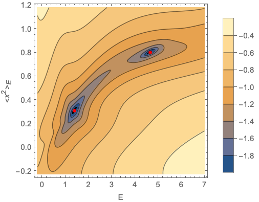
Figure 1: The $\eta_{\text{min}}$ landscape for the Hermitian Hamiltonian $H=p^{2}+x^{2}+x^{4}$ with $K=2,L=4$. The two local minima correspond to the ground state and the first excited state. We plot $\log_{10}\eta_{\text{min}}$ as a function of the energy $E$ and the expectation value $\langle x^{2}\rangle_{E}$. As a height function, $\eta_{\text{min}}$ increases rapidly outside of the presented region. We use black color to denote the region with $\eta_{\text{min}}<10^{-2}$. The exact solutions are indicated by the red points.

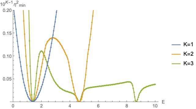
Figure 2: The minimized $\eta$ as a function of energy $E$ with the Hermitian Hamiltonian $H=p^{2}+x^{2}+x^{4}$ and $L=K+2$. The degrees of the polynomial approximations for null states are $K=1,2,3$. We carry out the minimization with respect to $\langle x^{2}\rangle$ as well. As we increase $K$, the minima give sharper predictions and capture more excited states. Here we change the weight in (8) to one.

$\Delta E_{n}^{(K)}$	$K=1$	$K=2$	$K=3$	$K=4$
$n=0$	$-1\times 10^{-3}$	$-2\times 10^{-3}$	$-4\times 10^{-10}$	$-7\times 10^{-12}$
$n=1$		$3\times 10^{-3}$	$-3\times 10^{-5}$	$2\times 10^{-11}$
$n=2$			$5\times 10^{-6}$	$6\times 10^{-7}$
$n=3$				$1\times 10^{-7}$

Table 1: The null bootstrap predictions for the low-lying energies of anharmonic oscillator with the Hermitian potential $V(x)=x^{2}+x^{4}$ and $L=K+2$. We present the first digit of the error $\Delta E^{(K)}_{n}=E^{(K)}_{n}-E^{\star}_{n}$. The reference energies $E_{0}^{\star}=1.39235164153029$, $E_{1}^{\star}=4.648812704212$, $E_{2}^{\star}=8.65504995776$ and $E_{3}^{\star}=13.1568038980$ are computed from diagonalizing the Hamiltonian with size $60\times 60$ in the basis of harmonic oscillator eigenfunctions.

$\Delta\langle x^{2}\rangle_{n}^{(K)}$	$K=1$	$K=2$	$K=3$	$K=4$
$n=0$	$-1\times 10^{-2}$	$-1\times 10^{-4}$	$2\times 10^{-9}$	$1\times 10^{-11}$
$n=1$		$1\times 10^{-3}$	$-1\times 10^{-6}$	$1\times 10^{-11}$
$n=2$			$-3\times 10^{-6}$	$6\times 10^{-8}$
$n=3$				$2\times 10^{-8}$

Table 2: The null bootstrap predictions for $\langle x^{2}\rangle_{n}$ with the Hermitian potential $V(x)=x^{2}+x^{4}$ and $L=K+2$. We present the first digit of the error $\Delta\langle x^{2}\rangle_{n}^{(K)}=\langle x^{2}\rangle^{(K)}_{n}-\langle x^{2}\rangle^{\star}_{n}$. The reference values $\langle x^{2}\rangle_{0}^{\star}=0.3058136507176$, $\langle x^{2}\rangle_{1}^{\star}=0.8012505955411$, $\langle x^{2}\rangle_{2}^{\star}=1.155440519200$ and $\langle x^{2}\rangle_{3}^{\star}=1.4675232154$ are computed using approximate wave functions from the diagonalization of the Hamiltonian with size $60\times 60$ in the harmonic oscillator basis.

Instead of rigorous bounds in the positive bootstrap, the null bootstrap gives an $\eta_{\text{min}}$ landscape. At the price of rigorousness, the null bootstrap results are more precise than those of the positive bootstrap. For instance, the size of the $E_{0}$ error bar from the rigorous island is $\delta E_{0}^{(K)}=\infty,3\times 10^{-2},1\times 10^{-4},5\times 10^{-10}$ with $K=1,2,3,4$. In the positive bootstrap, one asks if the positivity condition is violated and there is no smooth change in the answer. Then it requires some care to determine the boundaries of the positive regions, especially when an isolated region has a tiny size. In the null bootstrap, it is relatively easy to find the local minima thanks to the smooth $\eta_{\text{min}}$ landscape.

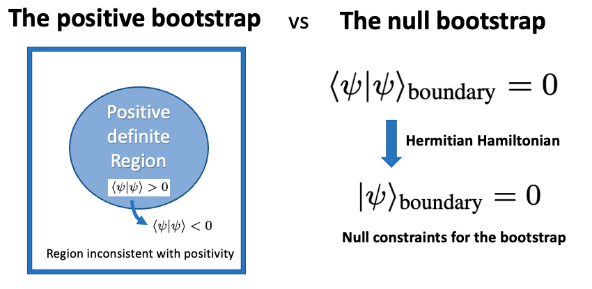
Figure 3: The relation between the positive and null bootstrap methods. For Hermitian Hamiltonians, the positive bootstrap results can be deduced by the null bootstrap method. Along a path in the parameter space, the norm of some state $|\psi\rangle$ changes sign after crossing the boundary of the positive region. The zero-norm states on the boundary should be null in the Hermitian theories, so the positive boundary can be studied directly by the null bootstrap.

Before moving to the non-Hermitian case, let us explain in Fig. 3 from a different perspective why the positive bootstrap results can be derived from the null bootstrap. In the positive bootstrap, one finds some regions satisfying the positive semidefinite condition. For some state, the norm will change sign after crossing a boundary, so it has zero norm precisely at the crossing point. In Hermitian systems, zero-norm states must be null, i.e. they should be orthogonal to the positive norm states. Therefore, we can directly search for the boundary of positive solutions using the null bootstrap. For the case of (10), we expect the positive islands shrink to points as $K$ goes to infinity, so they are captured by the local minima of the $\eta$ function.

IV.2 $V(x)=igx^{3}$

Since we propose that nullness is a more general principle than positivity, we should apply the null bootstrap to a non-positive system. Here we consider a simple non-Hermitian Hamiltonian

$$H=p^{2}+igx^{3}\,,$$ (11)

which is $\mathcal{PT}$ symmetric, i.e. invariant under the space–time reflection. We will set $g=1$ in the concrete computation.

In the textbooks of quantum mechanics, a standard axiom is that a fundamental Hamiltonian is Hermitian. The Hermiticity assumption ensures that the energy spectrum is real and the Hermitian norm is non-negative. Furthermore, the eigenfunctions are guaranteed to be orthogonal and complete.

For non-Hermitian Hamiltonians, the Hermitian norm does not need to have a definite sign , but Bessis and Zinn-Justin noticed that the Hamiltontian (11) may have a real energy spectrum. Their unpublished numerical study was motivated by the properties of the Yang-Lee edge singularities, whose critical behaviour is described by the $i\phi^{3}$ quantum field theory. It was later shown by Bender and Boettcher that the energy spectrum is real for a large class of non-Hermitian Hamiltonians with unbroken $\mathcal{PT}$ symmetry Bender:1998ke . Curiously, an imaginary cubic coupling constant also appeared in the study of Reggeon field theory Gribov:1967vfb .

When $g$ is small, the Hermitian case (10) can be viewed as a deformation of the harmonic oscillator, so it seems natural to find qualitatively similar results. By contrast, the non-Hermitian case (11) has no mass term and cannot be viewed as a deformed harmonic oscillator. Without knowing much about the lowering operators and spectra, it is a leap of faith to apply the null bootstrap to the non-Hermitian system (11). Surprisingly, the results of the $\eta$ minimization again exhibit a similar pattern.

$\Delta E_{n}^{(K)}$	$K=1$	$K=2$	$K=3$
$n=0$	$4\times 10^{-4}$	$-8\times 10^{-7}$	$1\times 10^{-11}$
$n=1$		$2\times 10^{-3}$	$-3\times 10^{-9}$
$n=2$			$-1\times 10^{-4}$

Table 3: The null bootstrap predictions for the low-lying energies of anharmonic oscillator with the non-Hermitian Hamiltonian $H=p^{2}+ix^{3}$ and $L=K+1$. The errors are defined as $\Delta E^{(K)}_{n}=E^{(K)}_{n}-E^{\star}_{n}$ and we present only the first digits. The reference energies $E_{0}^{\star}=1.156267072$, $E_{1}^{\star}=4.109228752$, $E_{2}^{\star}=7.562273854$ were obtained with the Runge-Kutta method in Bender:2007nj . A more precise value $E_{0}^{\star}=1.156267071988$ is computed by diagonalizing the Hamiltonian with size $60\times 60$.

$\Delta\langle x\rangle_{n}^{(K)}$	$K=1$	$K=2$	$K=3$
$n=0$	$-3\times 10^{-2}i$	$2\times 10^{-6}i$	$-2\times 10^{-11}i$
$n=1$		$-8\times 10^{-4}i$	$1\times 10^{-8}i$
$n=2$			$2\times 10^{-6}i$

Table 4: The null bootstrap predictions for $\langle x\rangle_{n}$ with the non-Hermitian potential $V(x)=ix^{3}$ and $L=K+1$. The errors are defined as $\Delta\langle x\rangle^{(K)}_{n}=\langle x\rangle^{(K)}_{n}-\langle x\rangle^{\star}_{n}$ and only the first digits are provided. The reference values $\langle x\rangle_{0}^{\star}=-0.590072533091i$, $\langle x\rangle_{1}^{\star}=-0.9820718380i$, $\langle x\rangle_{2}^{\star}=-1.20548075i$ were obtained by diagonalizing the Hamiltonian of size $60\times 60$.

After solving the consistency relations (1), we can express $\langle x^{m}p^{n}\rangle_{E}$ in terms of $\{E,\langle x\rangle_{E},\langle 1\rangle_{E}\}$. We again set $\langle 1\rangle_{E}=1$. However, this choice does not guarantee the non-negativity of the $\mathcal{PT}$ norm. As in the Hermitian example, the $\eta$ minimization for the non-Hermitian Hamiltonian (11) also captures more excited states as $K$ increases. In Table 3 and 4, we present the $\eta$ minimization results of the low-lying energy spectrum and the corresponding $\langle x\rangle=i\,\text{Im}\langle x\rangle$. Again, the precision increases rapidly with the cutoff parameter $K$. We set $a_{00}=0$ at $K=3$ to avoid the trivial solution $\mathcal{O}^{\text{trivial}}_{\text{null}}=H-E$.

Above, we successfully derived the real spectrum of the complex Hamiltonian (11) using the $\eta$ minimization. A curious question is: Are there $\eta$ minima with complex energies? It turns out that there indeed exist conjugate pairs of local minima with complex $E$ and complex $\langle x\rangle_{E}$. These minima persist as we increase $L-K$, so they should not be numerical coincidences. They might be related to other boundary conditions for the wave functions, but we do not fully understand the physical implications of these complex solutions.

V Ladder operators and matrix elements

In the previous section, we have derived the precise values of low-lying spectra $E_{n}$ and expectation values $\langle\psi_{E}|x^{m}p^{n}|\psi_{E}\rangle$ using the null bootstrap. Can we also compute the non-diagonal matrix elements? To address this question, let us remind the reader that we have introduced the ladder operators in Sec. III, which generate different energy eigenstates from a given one

$$|\psi_{E^{\prime}}\rangle=L_{E^{\prime}E}|\psi_{E}\rangle\,.$$ (12)

If one can determine the expressions of ladder operators, then the matrix elements are not independent parameters

$$\langle\psi_{E}|x^{m}p^{n}|\psi_{E^{\prime}}\rangle=\langle x^{m}p^{n}L_{E^{\prime}E}\rangle_{E}\,.$$ (13)

We will again approximate the ladder operators by finite degree polynomials

$$L^{(M)}_{E^{\prime}E}=\sum_{m=0}^{M}\sum_{n=0}^{M-m}c_{mn}\,x^{m}(ip)^{n}\,.$$ (14)

The coefficients $c_{mn}$ are determined by the $\eta$ minimization for the null constraints

$$\langle\psi_{\text{test}}^{(L)}|(H-E^{\prime})L^{(M)}_{E^{\prime}E}|\psi_{E}\rangle\approx 0\,,$$ (15)

which is an approximate version of the Schrödinger-like equation (4). We will choose a normalization such that the absolute norm of $|\psi_{E^{\prime}}\rangle$ is one and the signs of the lowest non-diagonal matrix elements are positive.

In Fig.5, we present some results of the quartic potential (10) based on the $K=4$ results. Naturally, the low-lying observables are more precise than the high-lying ones. For $M<K$, one can see that the results improve with the approximation order $M$. If $M>K$, the precision will decrease as the input parameters were derived from a truncation of order-$K$.

$\Delta\langle 0|x^{m}|n\rangle^{(M)}$	$m=1$	$m=2$	$m=3$	$m=4$
$n=1,M=1$	$4\times 10^{-6}$		$1\times 10^{-5}$
$n=2,M=2$		$3\times 10^{-7}$		$1\times 10^{-6}$
$n=1,M=3$	$1\times 10^{-11}$		$2\times 10^{-11}$

Table 5: The null bootstrap predictions for the low-lying matrix elements of anharmonic oscillator with the Hermitian potential $V(x)=x^{2}+x^{4}$. We use a shorthand notation $\langle 0|x^{m}|n\rangle=\langle\psi_{E_{0}}|x^{m}|\psi_{E_{n}}\rangle$. The differences are defined as $\Delta\langle 0|x^{m}|n\rangle^{(M)}=\langle 0|x^{m}|n\rangle^{(M)}-\langle 0|x^{m}|n\rangle^{\star}$. The reference values from the Hamiltonian diagonalization are $\langle 0|x^{1}|1\rangle^{\star}=0.552565959314$, $\langle 0|x^{3}|1\rangle^{\star}=0.456180404562$, $\langle 0|x^{2}|2\rangle^{\star}=0.406699817396$, $\langle 0|x^{4}|2\rangle^{\star}=0.62270464561$. Some matrix elements should vanish due to the unbroken parity symmetry of the energy eigenstates. Their numerical values are of order $10^{-11}$ or smaller, which are not presented here.

Since the parity symmetry of (10) is unbroken, the ladder operators have numerically small coefficients for the parity violating terms. For example, the numerical coefficients of $1,x^{2},p^{2},xp$ in $L_{E_{1},E_{0}}^{(M=3)}$ are of order $10^{-15}$. We do not present the results of $n=1,M=2$ in Table 5, because the precision is similar to the case of $n=1,M=1$. These parity constraints also explain the precision pattern of Table 1 and 2 as we increase $K$. For consistency, the parity-forbidden matrix elements indeed take negligible numerical values. In addition, we have also verified the approximate orthogonality of different eigenstates, i.e. $\langle 0|n\rangle^{(M)}\approx 0$ for $n>0$.

For the completeness of eigenfunctions, it is natural that the party of $|n\rangle$ is given by $(-1)^{n}$ as in the harmonic case. Then the level-$j$ ladder operator that connects $|n\rangle$ and $|n+j\rangle$ should consist of only parity-even (odd) monomials for even (odd) $j$. This also applies to the non-Hermitian case of $V(x)=igx^{3}$: The terms violating $\mathcal{PT}$-symmetry make negligible contributions to the ladder operators, as they should be composed of monomials with the same $\mathcal{PT}$ eigenvalues, up to a phase factor . By taking into account the global symmetry, the polynomial ansatz of (14) takes a more restricted form.

We can further study the algebraic properties of the ladder operators using their approximate expressions. Although $L^{(M)}_{EE^{\prime}}L^{(M)}_{E^{\prime}E}$ are finite degree polynomials with non-zero expectation values, we observe that

$$\langle\mathcal{O}^{(L)}_{\text{test}}\,[H,L^{(M)}_{EE^{\prime}}L^{(M)}_{E^{\prime}E}]\rangle_{E}\approx 0\,,$$ (16)

so these commutators are close to a linear combination of null operators. Note that $L^{(M)}_{EE^{\prime}}$ is not derived from the Hermitian conjugation of $L^{(M)}_{E^{\prime}E}$. The action of $L_{E^{\prime}E}$ and then $L_{EE^{\prime}}$ on $|\psi_{E}\rangle$ should leave it invariant up to some numerical factor. These product operators $L_{EE^{\prime}}L_{E^{\prime}E}$ can be interpreted as the interacting counterparts of the number operator of harmonic oscillator.

VI Discussion

In this work, we proposed the principle of nullness for bootstrapping quantum systems. The existence of many null state conditions can guarantee that the energy spectrum is bounded from below, so the quantum system is stable. As concrete examples, we use the $\eta$ minimization to obtain high precision results for both Hermitian and non-Hermitian anharmonic oscillators.

It would be interesting to apply the null bootstrap to quantum many body problems. Recently, the positive bootstrap has made some initial steps in this direction Han:2020 ; Lawrence:2021msm . Since we argue that the null bootstrap can deduce the positive bootstrap results, it should also furnish a new method for studying many important but challenging lattice models, ranging from high energy physics to condensed matter physics.

Previously, we constrained the Ising and Yang-Lee CFT data by imposing the operator decoupling in the intermediate spectrum of identical correlators Li:2017agi . In light of the results in this work, it would be interesting to consider a system of correlators such that their superposition gives rise to an external null state. This approach can be viewed as a $d>2$ generalization of the Virasoro null state constraints on correlators that lead to the Belavin-Polyakov-Zamolodchikov differential equations.

In the end, we list some questions that we find interesting:

• Can we interpret the large number of null state conditions as a kind of “integrability”? It would be interesting to further study the algebraic properties of the null and ladder operators. At the end of Sec. V, we presented some preliminary results concerning this question.

• Our bootstrap study is based on the operator-algebra formulation and we do not use the explicit expressions of the eigenfunctions. What are the algebraic counterparts of many important concepts in the wave function formulation, such as boundary conditions, Stokes sectors and WKB method?

• The non-Hermitian models can be extended to non-integer powers. Can we also study them from the bootstrap perspective? This will require the introduction of non-integer “power” to the operator algebra. This is closely related to the analyticity of the expectation values.

• Can a physical operator algebra has a bounded-from-below representation without resorting to some null state conditions? So the vacuum state is NOT annihilated by any lowering operators?

• Projection techniques play a significant role in both high energy physics and condensed matter physics, such as the GSO projection in superstring theories Gliozzi:1976qd and projective construction of quantum spin-liquid states Wen:2004ym . Can we view them as special cases of the nullness principle and make more general classifications?

- (1) S. Ferrara, A. F. Grillo and R. Gatto, “Tensor representations of conformal algebra and conformally covariant operator product expansion,” Annals Phys. 76, 161 (1973). doi:10.1016/0003-4916(73)90446-6
- (2) A. M. Polyakov, “Nonhamiltonian approach to conformal quantum field theory,” Zh. Eksp. Teor. Fiz. 66, 23 (1974) [Sov. Phys. JETP 39, 9 (1974)].
- (3) A. A. Belavin, A. M. Polyakov and A. B. Zamolodchikov, “Infinite Conformal Symmetry in Two-Dimensional Quantum Field Theory,” Nucl. Phys. B 241, 333 (1984). doi:10.1016/0550-3213(84)90052-X
- (4) P. Di Francesco, P. Mathieu and D. Senechal, “Conformal Field Theory,” doi:10.1007/978-1-4612-2256-9
- (5) R. Rattazzi, V. S. Rychkov, E. Tonni and A. Vichi, “Bounding scalar operator dimensions in 4D CFT,” JHEP 0812, 031 (2008) doi:10.1088/1126-6708/2008/12/031 [arXiv:0807.0004 [hep-th]].
- (6) S. El-Showk, M. F. Paulos, D. Poland, S. Rychkov, D. Simmons-Duffin and A. Vichi, “Solving the 3D Ising Model with the Conformal Bootstrap,” Phys. Rev. D 86, 025022 (2012) doi:10.1103/PhysRevD.86.025022 [arXiv:1203.6064 [hep-th]].
- (7) S. El-Showk, M. F. Paulos, D. Poland, S. Rychkov, D. Simmons-Duffin and A. Vichi, “Solving the 3d Ising Model with the Conformal Bootstrap II. c-Minimization and Precise Critical Exponents,” J. Stat. Phys. 157, 869 (2014) doi:10.1007/s10955-014-1042-7 [arXiv:1403.4545 [hep-th]].
- (8) F. Kos, D. Poland and D. Simmons-Duffin, “Bootstrapping Mixed Correlators in the 3D Ising Model,” JHEP 1411, 109 (2014) doi:10.1007/JHEP11(2014)109 [arXiv:1406.4858 [hep-th]].
- (9) F. Kos, D. Poland, D. Simmons-Duffin and A. Vichi, “Precision Islands in the Ising and Models,” JHEP 1608, 036 (2016) doi:10.1007/JHEP08(2016)036 [arXiv:1603.04436 [hep-th]].
- (10) P. D. Anderson and M. Kruczenski, “Loop Equations and bootstrap methods in the lattice,” Nucl. Phys. B 921, 702-726 (2017) doi:10.1016/j.nuclphysb.2017.06.009 [arXiv:1612.08140 [hep-th]].
- (11) H. W. Lin, “Bootstraps to strings: solving random matrix models with positivity,” JHEP 06, 090 (2020) doi:10.1007/JHEP06(2020)090 [arXiv:2002.08387 [hep-th]].
- (12) X. Han, S. A. Hartnoll and J. Kruthoff, “Bootstrapping Matrix Quantum Mechanics,” Phys. Rev. Lett. 125, no.4, 041601 (2020) doi:10.1103/PhysRevLett.125.041601 [arXiv:2004.10212 [hep-th]].
- (13) X. Han, “Quantum Many-body Bootstrap,” [arXiv:2006.06002[cond-mat]].
- (14) V. Kazakov and Z. Zheng, “Analytic and numerical bootstrap for one-matrix model and “unsolvable” two-matrix model,” JHEP 06 (2022), 030 doi:10.1007/JHEP06(2022)030 [arXiv:2108.04830 [hep-th]].
- (15) D. Berenstein and G. Hulsey, “Bootstrapping Simple QM Systems,” [arXiv:2108.08757 [hep-th]].
- (16) J. Bhattacharya, D. Das, S. K. Das, A. K. Jha and M. Kundu, “Numerical bootstrap in quantum mechanics,” Phys. Lett. B 823, 136785 (2021) doi:10.1016/j.physletb.2021.136785 [arXiv:2108.11416 [hep-th]].
- (17) Y. Aikawa, T. Morita and K. Yoshimura, “Application of bootstrap to a term,” Phys. Rev. D 105 (2022) no.8, 085017 doi:10.1103/PhysRevD.105.085017 [arXiv:2109.02701 [hep-th]].
- (18) D. Berenstein and G. Hulsey, “Bootstrapping more QM systems,” J. Phys. A 55 (2022) no.27, 275304 doi:10.1088/1751-8121/ac7118 [arXiv:2109.06251 [hep-th]].
- (19) S. Tchoumakov and S. Florens, “Bootstrapping Bloch bands,” J. Phys. A 55, no.1, 015203 (2022) doi:10.1088/1751-8121/ac3c82 [arXiv:2109.06600 [cond-mat.mes-hall]].
- (20) Y. Aikawa, T. Morita and K. Yoshimura, “Bootstrap method in harmonic oscillator,” Phys. Lett. B 833 (2022), 137305 doi:10.1016/j.physletb.2022.137305 [arXiv:2109.08033 [hep-th]].
- (21) B. n. Du, M. x. Huang and P. x. Zeng, “Bootstrapping Calabi–Yau quantum mechanics,” Commun. Theor. Phys. 74 (2022) no.9, 095801 doi:10.1088/1572-9494/ac679a [arXiv:2111.08442 [hep-th]].
- (22) S. Lawrence, “Bootstrapping Lattice Vacua,” [arXiv:2111.13007 [hep-lat]].
- (23) D. Bai, “Bootstrapping the deuteron,” [arXiv:2201.00551 [nucl-th]].
- (24) Y. Nakayama, “Bootstrapping microcanonical ensemble in classical system,” Mod. Phys. Lett. A 37 (2022) no.09, 2250054 doi:10.1142/S0217732322500547 [arXiv:2201.04316 [hep-th]].
- (25) J. L. Cardy, “Conformal Invariance and the Yang-lee Edge Singularity in Two-dimensions,” Phys. Rev. Lett. 54, 1354-1356 (1985) doi:10.1103/PhysRevLett.54.1354
- (26) J. L. Cardy and G. Mussardo, “S Matrix of the Yang-Lee Edge Singularity in Two-Dimensions,” Phys. Lett. B 225, 275-278 (1989) doi:10.1016/0370-2693(89)90818-6
- (27) D. Friedan, Z. a. Qiu and S. H. Shenker, “Conformal Invariance, Unitarity and Two-Dimensional Critical Exponents,” Phys. Rev. Lett. 52, 1575-1578 (1984) doi:10.1103/PhysRevLett.52.1575
- (28) M. E. Fisher, “Yang-Lee Edge Singularity and phi**3 Field Theory,” Phys. Rev. Lett. 40, 1610-1613 (1978) doi:10.1103/PhysRevLett.40.1610
- (29) W. Li, “New method for the conformal bootstrap with OPE truncations,” [arXiv:1711.09075 [hep-th]].
- (30) F. Gliozzi, “More constraining conformal bootstrap,” Phys. Rev. Lett. 111, 161602 (2013) doi:10.1103/PhysRevLett.111.161602 [arXiv:1307.3111 [hep-th]].
- (31) W. Li, “Ising model close to d=2,” Phys. Rev. D 105 (2022) no.9, L091902 doi:10.1103/PhysRevD.105.L091902 [arXiv:2107.13679 [hep-th]].
- (32) G. Kántor, V. Niarchos and C. Papageorgakis, “Solving Conformal Field Theories with Artificial Intelligence,” Phys. Rev. Lett. 128, no.4, 041601 (2022) doi:10.1103/PhysRevLett.128.041601 [arXiv:2108.08859 [hep-th]].
- (33) G. Kántor, V. Niarchos and C. Papageorgakis, “Conformal bootstrap with reinforcement learning,” Phys. Rev. D 105, no.2, 025018 (2022) doi:10.1103/PhysRevD.105.025018 [arXiv:2108.09330 [hep-th]].
- (34) C. M. Bender and T. T. Wu, “Anharmonic oscillator,” Phys. Rev. 184, 1231-1260 (1969) doi:10.1103/PhysRev.184.1231
- (35) M. Reehorst, S. Rychkov, D. Simmons-Duffin, B. Sirois, N. Su and B. van Rees, “Navigator Function for the Conformal Bootstrap,” SciPost Phys. 11, 072 (2021) doi:10.21468/SciPostPhys.11.3.072 [arXiv:2104.09518 [hep-th]].
- (36) C. M. Bender, D. C. Brody and H. F. Jones, “Complex extension of quantum mechanics,” Phys. Rev. Lett. 89, 270401 (2002) [erratum: Phys. Rev. Lett. 92, 119902 (2004)] doi:10.1103/PhysRevLett.89.270401 [arXiv:quant-ph/0208076 [quant-ph]].
- (37) S. Khan, Y. Agarwal, D. Tripathy and S. Jain, “Bootstrapping PT symmetric quantum mechanics,” Phys. Lett. B 834 (2022), 137445 doi:10.1016/j.physletb.2022.137445 [arXiv:2202.05351 [quant-ph]].
- (38) C. O. Nancarrow and Y. Xin, “Bootstrapping the gap in quantum spin systems,” [arXiv:2211.03819 [hep-th]].
- (39) C. M. Bender and S. Boettcher, “Real spectra in nonHermitian Hamiltonians having PT symmetry,” Phys. Rev. Lett. 80, 5243-5246 (1998) doi:10.1103/PhysRevLett.80.5243 [arXiv:physics/9712001 [physics]].
- (40) V. N. Gribov, “A REGGEON DIAGRAM TECHNIQUE,” Zh. Eksp. Teor. Fiz. 53, 654-672 (1967)
- (41) C. M. Bender, “Making sense of non-Hermitian Hamiltonians,” Rept. Prog. Phys. 70, 947 (2007) doi:10.1088/0034-4885/70/6/R03 [arXiv:hep-th/0703096 [hep-th]].
- (42) W. Li, “Inverse Bootstrapping Conformal Field Theories,” JHEP 01, 077 (2018) doi:10.1007/JHEP01(2018)077 [arXiv:1706.04054 [hep-th]].
- (43) P. Dorey and R. Tateo, “Anharmonic oscillators, the thermodynamic Bethe ansatz, and nonlinear integral equations,” J. Phys. A 32, L419-L425 (1999) doi:10.1088/0305-4470/32/38/102 [arXiv:hep-th/9812211 [hep-th]].
- (44) D. J. Binder and S. Rychkov, “Deligne Categories in Lattice Models and Quantum Field Theory, or Making Sense of Symmetry with Non-integer ,” JHEP 04, 117 (2020) doi:10.1007/JHEP04(2020)117 [arXiv:1911.07895 [hep-th]].
- (45) F. Gliozzi, J. Scherk and D. I. Olive, “Supersymmetry, Supergravity Theories and the Dual Spinor Model,” Nucl. Phys. B 122, 253-290 (1977) doi:10.1016/0550-3213(77)90206-1
- (46) X. G. Wen, “Quantum field theory of many-body systems: From the origin of sound to an origin of light and electrons,”