Log-based Anomaly Detection with Deep Learning:
How Far Are We?

Abstract.

Software-intensive systems produce logs for troubleshooting purposes. Recently, many deep learning models have been proposed to automatically detect system anomalies based on log data. These models typically claim very high detection accuracy. For example, most models report an F-measure greater than 0.9 on the commonly-used HDFS dataset. To achieve a profound understanding of how far we are from solving the problem of log-based anomaly detection, in this paper, we conduct an in-depth analysis of five state-of-the-art deep learning-based models for detecting system anomalies on four public log datasets. Our experiments focus on several aspects of model evaluation, including training data selection, data grouping, class distribution, data noise, and early detection ability. Our results point out that all these aspects have significant impact on the evaluation, and that all the studied models do not always work well. The problem of log-based anomaly detection has not been solved yet. Based on our findings, we also suggest possible future work.

1. Introduction

High availability and reliability are essential for large-scale software-intensive systems. As these systems provide various services to a large number of users, a small problem in the system could lead to user dissatisfaction and even significant financial loss. Anomaly detection is, therefore, important for the quality assurance of complex software-intensive systems.

Software-intensive systems often record runtime information by printing console logs. A large and complex system could produce a massive amount of logs, which can be used for troubleshooting purposes. For example, the cloud computing systems of Alibaba Inc. produce about 30-50 gigabytes (around 120-200 million lines) of tracing logs per hour (Mi et al., 2013). Log data is usually unstructured text messages, which can help engineers understand the system’s internal status and facilitate monitoring, administering, and troubleshooting of the system (He et al., 2020a). Log messages can be parsed into log events, which are templates (constant part) of the messages. Figure 1 shows an example of raw log messages and the corresponding log events obtained after parsing.

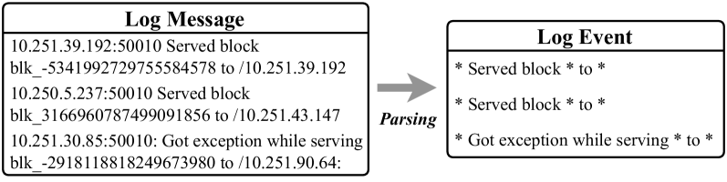
Figure 1. An example of log messages and log events

Over the years, many data-driven methods have been proposed to automatically detect system anomalies by analyzing log data (Breier and Branišová, 2015; Zhang et al., 2020; Du et al., 2017; Chen et al., 2004; Xu et al., 2009; Zhang et al., 2019; Lin et al., 2016). For example, He et al. (He et al., 2016) evaluated six popular machine learning (ML) algorithms for log-based anomaly detection. These ML-based methods share some limitations of inflexible features, inefficiency, and weak adaptability (Zhang et al., 2019). In order to address these issues, deep learning (DL) has been adopted and produced promising results. Du et al. (Du et al., 2017) proposed to use Long-Short Term Memory (LSTM) to model the sequential patterns of normal sessions, then identify anomalies as those violated the patterns. Meng et al. (Meng et al., 2019) trained an LSTM model to detect sequential and quantitative anomalies using log count vectors as inputs. They also proposed template2vec to consider the synonyms and antonyms of the words in log templates. Other studies (Zhang et al., 2019; Li et al., 2020) represent log templates as semantic vectors to handle the instability of log data. Generally, the existing DL-based log anomaly detection methods show promising results on commonly used datasets and claim their superiority over traditional ML-based approaches. For instance, DeepLog (Du et al., 2017) and LogAnomaly (Meng et al., 2019) all reported a very good performance on commonly-used HDFS and BGL datasets (with F-measure values greater than 0.9).

However, we notice that several important aspects are overlooked by the existing work. These aspects are associated with experimental datasets, evaluation metrics, and experimental settings. In this work, we would like to dive deep into the problem and answer: Are log-based anomaly detection methods with deep learning as good as they claimed? What are the major factors that could affect their performance?

To answer the above questions, we conduct a systematic evaluation of five representative deep learning models for log-based anomaly detection (including DeepLog (Du et al., 2017), LogAnomaly (Meng et al., 2019), PLELog (Yang et al., 2021), LogRobust (Zhang et al., 2019), and CNN (Lu et al., 2018)) on four datasets (including HDFS, BGL, Spirit, and Thunderbird), under controlled experimental settings. We first conduct an analysis of training data selection and grouping techniques. Then we explore the impact of different characteristics of datasets (including data noise and class distribution) on model performance. Finally, we analyze the ability of the models in the early detection of anomalies. Through extensive experiments, we obtain the following major findings about the current deep learning models for log-based anomaly detection:

• The training data selection strategies (random or chronological) have significant impact on the semi-supervised log-based anomaly detection models. Randomly selecting training data could cause the data leakage problem and unreasonably high detection accuracy.

• Different log data grouping methods have substantial influence on the performance of the models. Models tend to lose their accuracy when dealing with shorter log sequences.

• The effectiveness of the models is significantly affected by the highly imbalanced class distribution. Commonly-used metrics, including Precision, Recall, and F-measure, are not comprehensive enough for evaluating a log-based anomaly detection model with highly imbalanced data.

• A small amount of data noise, including mislabelled logs and log parsing errors can downgrade anomaly detection performance. Compared to semi-supervised methods, supervised models are more sensitive to mislabelled logs in the training data. Models capable of understanding the semantic meaning of log data could reduce the impact of log parsing errors.

• Different models have different abilities in the early detection of system anomalies. Some models can detect anomalies earlier than others.

In summary, the major contributions of this work are as follows:

• We conduct an extensive evaluation of five representative deep learning models for log-based anomaly detection.

• We conclude that the existing models are not evaluated comprehensively and do not generalize well in different experimental settings.

• Based on the evaluation results, we point out the advantages and disadvantages of existing models, and suggest future research work for log-based anomaly detection.

2. Log-based Anomaly Detection with Deep Learning

2.1. Representative Models

In recent years, many deep learning-based models have been proposed to analyze log data and detect anomalies (Breier and Branišová, 2015; Zhang et al., 2020; Du et al., 2017; Zhang et al., 2019; Nedelkoski et al., 2020; Yang et al., 2021; Li et al., 2020). Some of these models use supervised learning techniques (such as LogRobust (Zhang et al., 2019) and CNN (Lu et al., 2018)), while others employ semi-supervised approaches (such as DeepLog (Du et al., 2017), LogAnomaly (Meng et al., 2019)) or unsupervised approaches  (Farzad and Gulliver, 2020). Some recent representative models are as follows:

DeepLog. Du et al. (Du et al., 2017) proposed to utilize an LSTM model to learn the system’s normal executions by predicting the next log event given preceding events. It detects anomalies by determining whether or not an incoming log event violates the prediction results of the LSTM model. Their experimental results show that DeepLog can achieve an F-measure of 0.96 on the HDFS dataset.

LogAnomaly. Meng et al. (Meng et al., 2019) proposed LogAnomaly, which uses log count vectors as inputs to train an LSTM model. They also proposed template2vec, a synonyms and antonyms based method, to represent log templates as semantic vectors to match new log events with existing templates. Like DeepLog, a forecasting-based detection model is designed to predict the next log event, and if the examined log event violates the prediction results, it will be marked as an anomaly. LogAnomaly can achieve F-measures of 0.95 and 0.96 on HDFS and BGL datasets, respectively.

PLELog. Yang et al. (Yang et al., 2021) addressed the issue of insufficient labels via probabilistic label estimation and designed an attention-based GRU neural network to detect anomalies. The GRU-based detection model is built to classify log sequences into two classes, normal or abnormal. Their experimental results indicate that PLELog outperforms existing semi-supervised methods and achieves high performance on HDFS and BGL datasets (i.e., 0.96 and 0.98, respectively).

LogRobust. Zhang et al. (Zhang et al., 2019) incorporated a pre-trained Word2vec model, namely FastText (Joulin et al., 2016), and combined it with TF-IDF weights to learn the representation vectors of log templates. Then, these vectors were input to an Attention-based Bi-LSTM model to detect anomalies. The experimental results show that LogRobust can address the instability of log events and achieve F-measures of 0.99 on the original HDFS dataset and 0.89-0.96 on synthetic datasets.

CNN. Lu et al. (Lu et al., 2018) applied a Convolutional Neural Network (CNN) for log-based anomaly detection. Logs are grouped into sessions, then transformed into a trainable matrix. A CNN model is trained using this matrix as inputs to classify a log sequence into normal or abnormal. The CNN model can achieve an F-measure of 0.98 on the HDFS dataset.

In this study, we systematically evaluate the above five models. DeepLog and LogAnomaly adopt a forecasting-based approach (i.e., detecting anomalies by predicting the next log event given preceding log sequences), while PLELog, LogRobust, and CNN are classification-based models (i.e., detecting anomalies by classifying log sequences). Apart from these models, there are some other deep learning-based approaches. For example, Logsy (Nedelkoski et al., 2020) utilizes the Transformer network (Vaswani et al., 2017) to detect anomalies from log data. AutoEncoder has been employed in (Farzad and Gulliver, 2020) to detect log anomalies in an unsupervised manner along with Isolation Forest. SwissLog (Li et al., 2020) proposes to use a dictionary-based log parser and an Attention-based Bi-LSTM network to detect anomalies for diverse faults. As their source code is not publicly available, we do not experimentally evaluate these models in this study.

2.2. The Common Workflow

The common overall framework of DL models for log-based anomaly detection is shown in Figure 2. Generally, the framework consists of four steps: (1) log parsing, (2) log grouping, (3) log representation, (4) anomaly detection through DL models.

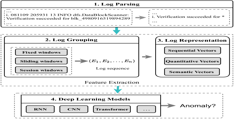
Figure 2. Log-based Anomaly Detection Workflow with Deep Learning: The Common Workflow

2.2.1. Log parsing

Logs are semi-structured texts, which contain various fields such as timestamp and severity. To favor downstream tasks, log parsing is applied to automatically convert each log message into a specific event template (constant part) associated with parameters (i.e., variable part). For example, the log template “Verification succeeded for $*$” can be extracted from the log message “Verification succeeded for blk_4980916519894289” in Figure 2. Here, “$*$” denotes the position of a parameter.

There are many log parsing techniques, based on frequent pattern mining (Nagappan and Vouk, 2010; Vaarandi and Pihelgas, 2015; Dai et al., 2020), clustering (Tang et al., 2011; Hamooni et al., 2016; Shima, 2016), and heuristics (He et al., 2017; Jiang et al., 2008; Makanju et al., 2009). The heuristics-based approaches make use of the characteristics of logs and have been found to perform better than other techniques in terms of accuracy and time efficiency (Zhu et al., 2019).

2.2.2. Log Grouping

The main purpose of this step is to separate logs into various groups, where each group represents a finite chunk of logs (He et al., 2016). These groups are called log sequences, from which features are extracted and fed into anomaly detection models. As introduced in (He et al., 2016), three types of windows are applied (see Figure 2) for log grouping, including: (1) Fixed window. Logs are grouped by fixed windows according to their occurrences. The occurrence is defined by the timestamp of log messages or by the order of its appearance in the dataset. Each window has a fixed size (i.e., window size), which means the time span or the number of logs. (2) Sliding window. Sliding windows consist of two attributes: window size and step size. The window size can be the time span or the number of logs in a log sequence, while the step size is the forwarding distance. (3) Session window. Different from fixed/sliding windows, session windows are based on the identifier of logs. Identifiers are used to group logs in the same execution path. For example, HDFS logs use block_id to record the execution path.

2.2.3. Log Representation

After log grouping, logs are represented in different formats required by DL models. Existing DL-based anomaly detection models convert logs into three main types: (1) sequential vectors, (2) quantitative vectors, and (3) semantic vectors. Sequential vectors reflect the order of log events in a window. For example, DeepLog (Du et al., 2017) assigns each log event with an index, then generates a sequential vector for each log window. Quantitative vectors are similar to log count vectors, which are used to hold the occurrence of each log event in a log window. LogAnomaly (Meng et al., 2019) leverages both sequential and quantitative vectors to detect anomalies. Different from them, semantic vectors are acquired from language models to represent the semantic meaning of log events. Each log window is converted into a set of semantic vectors for the detection models. For instance, LogRobust (Zhang et al., 2019) adopts a pre-trained FastText (Joulin et al., 2016) model to compute the semantic vectors of log events.

2.2.4. Deep Learning Models

After the log representation phase, the extracted features are fed to deep learning models for the anomaly detection task. A variety of DL techniques have been applied to log-based anomaly detection: 1) RNN. Recurrent Neural Networks (RNNs), including its variants Long Short-Term Memory (LSTM) (Hochreiter and Schmidhuber, 1997) and Gated Recurrent Units (GRUs) (Cho et al., 2014), are neural networks designed to handle the sequential inputs with arbitrary length. Bi-directional RNN is used to represent the sequential text in both directions (i.e., forward and backward). RNN and its variants have been applied in many studies on log-based anomaly detection. Specifically, DeepLog (Du et al., 2017) and LogAnomaly  (Meng et al., 2019) use LSTM to predict the next log event. LogRobust (Zhang et al., 2019) applies an Attention-based Bi-LSTM network to handle the instability of logs, while PLELog adopts GRUs to build a classification model. 2) CNN. A Convolutional Neural Network (CNN) uses convolution operation to extract meaningful local patterns of input. In  (Lu et al., 2018), a CNN model originally designed for sentence classification (Kim, 2014) is applied to log-based anomaly detection. 3) Transformer. The Transformer network has made significant progress in neural machine translation and related pretraining tasks in recent years. It has been applied in (Nedelkoski et al., 2020; Le and Zhang, 2021; Guo et al., 2021) for log-based anomaly detection.

3. Study Design

3.1. Motivation

Recent studies (Meng et al., 2019; Li et al., 2020) have shown that deep learning-based approaches can achieve high accuracy (e.g., F-Measure higher than 90%) on commonly used datasets (e.g., the HDFS dataset). These results seem to suggest that the problem of anomaly detection can be solved almost perfectly through deep learning. To explore the actual effectiveness of existing DL models for log-based anomaly detection ($models$ for short in the rest of the paper), we would like to evaluate the models from the following aspects associated with the common workflow of the models:

3.1.1. The selection of training data

The results of anomaly detection could be affected by the selection of training data. In some studies (such as DeepLog (Du et al., 2017), LogRobust (Zhang et al., 2019), PLELog (Yang et al., 2021), and CNN (Lu et al., 2018)), the training and test data are selected based on the timestamp of logs. We call it $chronological$ strategy. Other studies (Guo et al., 2021; Chen et al., 2021; Meng et al., 2019) apply fixed/sliding windows to group log events into log sequences, then shuffle all logs sequences before splitting them into training and testing sets. We call it $random$ strategy. The random strategy allows models to see more log events and achieve high accuracy (e.g., higher than 88% F-measure for all models (Chen et al., 2021)). However, this strategy may lead to the data leakage problem in the training phase. That is, it is possible that the training set contains parts of future data, and the testing set contains parts of past data, thus making it not suitable for real-world scenarios where we only use historical logs to build a detection model. The effectiveness of the models with different training data selection strategies (random or chronological) should be investigated.

3.1.2. The grouping of log data

The log data can be grouped into sequences by session, sliding, or fixed windows. Choosing a proper window size is challenging. For example, if the window size is small, the models face difficulty in capturing those anomalies that span multiple sequences. On the other hand, if the window size is large, log sequences might include multiple anomalies and confuse the detection scheme (Liu et al., 2021). In this work, we evaluate many window sizes, including the window sizes from 20 to 200 log messages as well as the window sizes of 0.5 hour and 1 hour, and also session window (He et al., 2016; Zhang et al., 2020).

3.1.3. The imbalanced class distribution

In literature, much research work (Zhang, 2008, 2009; Fenton and Ohlsson, 2000) has shown that in a large software system, the distribution of faults is skewed - that a small number of modules accounts for a large proportion of the faults. In our work, we find that the distribution of anomalies is also skewed. The anomalous log sequences usually account for the minority of the dataset, which can be only from 0.5% to 15% of a dataset, as shown in Section 3.3. The highly imbalanced data imposes challenges for anomaly detection. In general, it is difficult for a machine learning technique to identify a small number of anomalies from a large amount of logs. The imbalance between normal and abnormal classes could cause the model to perform poorly.

The highly imbalanced class distribution also has implications for evaluation metrics. The performance of log-based anomaly detection models is usually measured by Precision, Recall, and F-Measure  (Du et al., 2017; Zhang et al., 2019; Guo et al., 2021; Meng et al., 2019; He et al., 2016). However, previous studies (Zhang and Zhang, 2007) pointed out that prediction results may not always be satisfactory in the presence of imbalanced data distribution. In this work, we would like to explore if the commonly-used metrics can effectively evaluate the effectiveness of a log-based anomaly detection model under the scenario of imbalanced class distribution.

3.1.4. The quality of data

For the evaluation of log-based anomaly detection models, labeled data is required. The commonly-used public datasets (such as HDFS and BGL) are manually inspected and labeled by engineers. Data noise (false positives/negatives) may be introduced during the manual labeling process. Although the data noises only occupy a small portion of logs, they could downgrade the performance of existing models. The noise can be from the errors in the preprocessing phase (i.e., log parsing). The logging statements could also frequently change during software evolution, resulting in new log events that were not seen in the training phase (Zhang et al., 2019; Meng et al., 2019). Zhang et al. (Zhang et al., 2019) found that 30.3% of logs are changed in the latest version based on their empirical study on Microsoft online service systems. Le et al. (Le and Zhang, 2021) found that log parsing errors can lead to many incorrect log events, thus downgrading anomaly detection performance. Therefore, we would like to investigate the effectiveness of the models with different degrees of data noise.

3.1.5. Early detection ability

System anomalies can affect the normal operations of upper-layer software applications and significantly affect users’ experience. If no actions are taken, more severe problems or even service interruptions may occur. Therefore, it is important that the anomalies are captured earlier, so that more mitigation actions could be taken. An effective anomaly detection model should be able to identify the early signals of system anomalies, detect the anomalies as early as possible, and meanwhile achieve high detection accuracy. This is especially essential for the online detection scenario, where anomalies are detected on the fly.

Because of the above concerns, we argue that the capabilities of deep learning-based techniques for anomaly detection should be re-evaluated. In this work, we design experiments to measure the impact of these factors on five representative DL models for log-based anomaly detection.

3.2. Evaluated Models

In this study, we evaluate the five representative models described in Section 2.1, namely DeepLog, LogAnomaly, PLELog, LogRobust, and CNN. These models have their source code publicly available, and we can confirm the correctness of source codes by reproducing results presented in their original paper. Specifically, we adopt the public implementations (wuy, 2021; don, 2021) of DeepLog and LogAnomaly. For LogAnomaly, the template2vec model is trained with domain-specific antonyms and synonyms adding by operators. Since this information is unavailable, we use a pre-trained FastText word2vec mode (Joulin et al., 2016) to compute the semantic vectors of log templates. The template vector is calculated as the weighted average of the vectors of the template’s words. For LogRobust, we adopt the implementation provided by its authors and convert it into a PyTorch-based implementation. For PLELog, we leverage its public implementation (ple, 2021). For models whose hyperparameter settings are reported in their paper, we use the same hyperparameter values. Otherwise, we tune their hyperparameters empirically.

3.3. Datasets

To evaluate the studied models for log-based anomaly detection, we select four public datasets (log, 2021a; He et al., 2020b), namely HDFS, BGL, Thunderbird, and Spirit. The details of each dataset are as follows:

• HDFS (Hadoop Distributed File System) dataset is produced from more than 200 Amazon EC2 nodes. In total, the HDFS dataset consists of 11,175,629 log messages. These log messages form different log windows according to their block_id, reflecting a program execution in the HDFS system. There are 16,838 blocks of logs (2.93%) in this dataset indicating system anomalies.

• BGL (Blue Gene/L) dataset is a supercomputing system log dataset collected by Lawrence Livermore National Labs (LLNL) (Oliner and Stearley, 2007). The dataset contains 4,747,963 log messages. Each message in the BGL dataset was manually labelled as either normal or anomalous. There are 348,460 log messages (7.34%) that were labelled as anomalous.

• Spirit dataset is an aggregation of system log data from the Spirit supercomputing system at Sandia National Labs (Oliner and Stearley, 2007). There are more than 172 million log messages labeled as anomalous on the Spirit dataset. In this paper, we use a small set containing the first 5 million log lines of the original Spirit dataset, which contains 764,500 abnormal log messages (15.29%).

• Thunderbird dataset is an open dataset of logs collected from a Thunderbird supercomputer at Sandia National Labs (SNL) (Oliner and Stearley, 2007). The log data contains normal and abnormal messages which are manually identified. Thunderbird is a large dataset of more than 200 million log messages. We leverage 10 million continuous log lines for computation-time purposes, which contain 4,934 abnormal log messages (0.49%).

Table 1 summarizes the statistics of datasets used in our experiments.

Table 1. The statistics of datasets used in the experiments

Dataset	# Log Events	Grouping	# Log sequences	# Avg. seq. length	Training Data		Testing Data
					# Log sequences	# Anomaly	# Log sequences	# Anomaly
HDFS	48	session (random)	575,061	19.4	460,048	13,521 (2.9%)	115,013	3,317 (2.9%)
BGL	1,847	1 hour (random)	3,606	1,307.1	2,884	536 (18.6%)	722	129 (17.9%)
		1 hour (chron.)	3,606	1,307.1	2,625	496 (18.9%)	981	171 (17.4%)
		100 logs (chron.)	47,135	100	37,708	4,009 (10.6%)	9,427	817 (8.7%)
		session (random)	69,252	68.1	55,401	25,066 (45.2%)	13,851	6,309 (45.5%)
Spirit	2,880	1 hour (random)	1,173	4,262.6	1,001	882 (88.11%)	172	71 (41.28%)
		1 hour (chron.)	1,173	4,279.0	938	760 (81.02%)	235	192 (81.7%)
		100 logs (chron.)	50,000	100	40,000	19,384 (48.5%)	10,000	346 (3.5%)
Thunderbird	4,992	1 hour (random)	209	47,651.5	167	42 (25.1%)	42	6 (14.29%)
		1 hour (chron.)	209	47,651.5	169	40 (23.7%)	40	8 (20.0%)
		100 logs (chron.)	99,593	100	79,674	816 (1.0%)	19,919	27 (0.1%)
Note: chron. denotes the chronological strategy.

3.4. Research Questions

The goal of this study is to analyze the performance of the representative deep learning models for log-based anomaly detection models. We design the following research questions in accordance with the evaluation aspects described in Section 3.1.

RQ1: How do the existing approaches perform with different training data selection strategies? We want to evaluate whether or not the studied models are able to achieve good accuracy with different training data selection strategies. To this end, we conduct experiments with two different strategies for training data selection: (1) Random selection: For each dataset, we first sort logs by timestamps, and then apply the fixed window grouping technique to generate log sequences. Next, these log sequences are shuffled, and split into training/testing sets with the ratio of 80:20. (2) Chronological selection: For each dataset, we utilize the first 80% of raw logs (that appear in chronological order) for training and the remaining 20% for testing. Next, we apply the fixed window grouping technique to generate log sequences. We do not shuffle the generated log sequences in this strategy. Therefore, we can guarantee that only historical logs are used in the training phase, and there are no future logs used in this phase.

In this RQ, we experiment on the BGL, Thunderbird, and Spirit datasets. The window size for fixed window grouping is set to 1 hour. As the HDFS dataset does not contain timestamp information, the chronological selection cannot be applied to HDFS, and thus it is not used in this RQ.

RQ2: How do the existing models perform with different data grouping methods? To evaluate the impact of different data grouping methods on the performance of anomaly detection models, we choose the following three data grouping methods, including: (1) fixed-window grouping with the window size of 1 hour (as used in RQ1) and 0.5 hour, (2) fixed-window grouping with the window size varying from 20 to 200 log messages, and (3) session window grouping. For the first case, we use BGL, Spirit, and Thunderbird datasets. For the case of session windows, we use block_id and node_id to group logs on HDFS and BGL datasets, respectively.

RQ3: Can the existing approaches work with different class distributions? As shown in Section 3.3, our subject datasets represent highly imbalanced class distributions with anomaly ratios that can be only 0.1% (i.e., on the Thunderbird dataset). To perform a more systematic evaluation, we simulate different imbalanced scenarios by randomly removing the normal/abnormal log sequences from the subject datasets. For a real-world production system, the number of anomalies is much less than the number of normal events (Lin et al., 2018; Zhang, 2008, 2009). Therefore, we vary the imbalance ratio from 0.1% to 15%, which indicates the percentage of anomalies in the dataset. In this way, we create six synthetic datasets with the imbalance ratio of 0.1%, 0.5%, 1%, 5%, 10%, and 15%.

RQ4: Can existing approaches work with different degrees of data noise? To evaluate the impact of mislabelled logs on the performance of the studied models, we randomly add some anomalies (from 1% to 10%) into the training data for semi-supervised methods. For supervised methods, we randomly change the label of a specific portion (from 1% to 10%) to simulate the mislabelled logs. In this way, we create five synthetic datasets with the mislabelled proportion of 1%, 2%, 5%, 8%, and 10%. Moreover, to measure the impact of noises from log parsing errors, we experiment with four commonly used log parsers, including Drain (He et al., 2017), Spell (Du and Li, 2016), AEL (Jiang et al., 2008), and IPLoM (Makanju et al., 2009).

RQ5: How early can the existing models detect anomalies in online detection? As described in Section 3.1.5, a model should not only detect anomalies precisely but also should be able to detect anomalies as early as possible so that more mitigation actions could be taken. Therefore, in this RQ, we evaluate the studied models on four datasets to investigate their ability in early detection of anomalies. To this end, we record the number of examined log messages before each model raises an anomaly alert for a log sequence, in the online detection setting.

3.5. Experimental Setup

In our experiments, we preprocess the log data and conduct DL-based anomaly detection as follows:

(1) Log Parsing. To extract log templates from log data, we use the log parser Drain (He et al., 2017) with the default parameter settings (log, 2021b). The log data is denoted by $L=\{l_{1},l_{2},...,l_{i},...,l_{N_{L}}\}$ and contains $N_{L}$ entries (i.e., lines) of log messages. Each log message $l_{i}$ is parsed into a log template $E(l_{i})$, which is denoted $e_{i}$ for short.

(2) Log Grouping. We apply session window to group logs in the HDFS dataset using block_id. Each session is labeled using ground truth. For other datasets (BGL, Spirit, and Thunderbird), we use the fixed window strategy to group log data into $N_{S}$ chunks (i.e., log sequences), denoted as $S=\{s_{1},s_{2},...,s_{u},...,s_{N_{S}}\}$, where $s_{u}=\{e_{i},e_{i+1},...,e_{j}\}$ is a set of log templates. According to the ground truth (labeled by domain engineers), a log sequence is abnormal if it contains an anomalous log message according to the ground truth (labeled by domain engineers). $F$ denotes the size of each log sequence. In this study, we vary the value of $F$ from 20, 100, 200 log messages, to 0.5 and 1 hour depending on each research question.

(3) Log Representation. Log sequences are now converted into numerical vectors, which can be input to a DL model. DeepLog transforms log sequences into sequential vectors by assigning each log event with an index. LogAnomaly leverages both sequential vectors and quantitative vectors to train the model. The occurrence of each log event is counted and forms the quantitative vectors, which represent the system execution behaviors (Meng et al., 2019). PLELog extracts the semantic vectors of log templates by using a pre-trained Glove model (Pennington et al., 2014). Similarly, LogRobust and CNN also convert log sequences into semantic vectors using a pre-trained word2vec model. We adopt the pre-trained FastText (Joulin et al., 2016) model to compute the semantic vectors for LogRobust and CNN.

(4) Deep Learning Model. In this step, depending on the method, a DL model is trained using the corresponding feature vectors generated from the previous phase. DeepLog and LogAnomaly have two LSTM layers with 128 neurons. LogRobust contains a two-layer Bi-LSTM with 128 neurons and an attention layer. PLELog utilizes a one-layer GRU network. CNN has three Convolutional layers with different filters and a max-pooling layer for feature extraction.

To avoid bias from randomness, we perform each experiment five times and report the average results. We conduct our experiments on a Windows Server 2012 R2 with Intel Xeon E5-2609 CPU, 128GB RAM, and an NVIDIA Tesla K40c.

3.6. Evaluation Metrics

To measure the effectiveness of models in anomaly detection, we use the Precision, Recall, Specificity, and F1-Score metrics, which are defined as follows:

• Precision: the percentage of correctly detected abnormal log sequences amongst all detected abnormal log sequences by the model. $Prec=\frac{TP}{TP+FP}$.

• Recall: the percentage of log sequences that are correctly identified as anomalies over all real anomalies. $Rec=\frac{TP}{TP+FN}$.

• Specificity: the percentage of log sequences that are correctly identified as normal over all real normal sequences.
  $Spec=\frac{TN}{TN+FP}$.

• F-Measure: the harmonic mean of Precision and Recall.
  $F1=\frac{2*Prec*Rec}{Prec+Rec}$.

TP (True Positive) is the number of abnormal log sequences the are correctly detected by the model. FP (False Positive) is the number of normal log sequences that are wrongly identified as anomalies. FN (False Negative) is the number of abnormal log sequences that are not detected by the model.

4. Results and Findings

4.1. RQ1: Performance with different training data selection strategies?

For RQ1, we apply fixed window grouping with the size of 1 hour to generate log sequences on BGL, Spirit, and Thunderbird datasets (see Table 1). The training data is selected by random or chronological selection. The experimental results are shown in Table 2.

We find that, for semi-supervised models (i.e., LogAnomaly, DeepLog, and PLELog), the results with random selection are much better than those with chronological selection. For example, DeepLog achieves an F-measure of 0.927 with the random selection of training data on the BGL dataset. When training and testing sets are separated by the time order (i.e., chronological selection), the F-measure drops to 0.426. The reason is that with random selection, the models can see future log events in the training phase (i.e., data leakage), therefore they can make more accurate predictions. Besides, DeepLog and LogAnomaly train the models using the index of log events (i.e., sequential and quantitative vectors) and ignore the semantic meaning of logs during the training phase. DeepLog marks any new log events as anomalies and produces many false alarms. LogAnomaly can simply match some unseen log events with those appearing in the training phase, but it is not adequate compared to those models that are trained through the semantic understanding of logs.

The supervised models (i.e., LogRobust and CNN) perform much better than the semi-supervised models on both strategies since the models are trained with a large amount of normal and abnormal data. For example, these two models achieve around 0.94 F-measure on the Thunderbird dataset with the chronological setting, while others perform poorly. Another reason for these results is the advantages of semantic vectors used by these models, which can identify the semantically similar log events and also distinguish different log events (Zhang et al., 2019). Still, we can see that in general the results with random selection are better than those with chronological selection.

Our experimental results confirm that models perform better with random selection. The data leakage problem is a reason for the good performance of some DL-based log anomaly detection models (e.g., LogAnomaly (Meng et al., 2019), which uses the random strategy in their evaluation). Due to this problem, we suggest that chronological selection should be applied to evaluate the effectiveness of the models in real-world scenarios. Hence, for other RQs, we will apply the chronological selection to group log messages.

Table 2. Comparison of model performance with random selection and chronological selection of training data

Model	BGL (random/chronological selection)				Spirit (random/chronological selection)				Thunderbird (random/chronological selection)
	Prec	Rec	Spec	F1	Prec	Rec	Spec	F1	Prec	Rec	Spec	F1
DeepLog	0.952/0.270	0.903/0.988	0.990/0.437	0.927/0.426	0.867/0.438	1.0/1.0	0.386/0.090	0.929/0.609	0.232/0.200	1.0/1.0	0.007/0	0.369/0.333
LogAnomaly	0.961/0.313	0.903/0.798	0.992/0.551	0.931/0.483	0.882/0.438	1.0/1.0	0.456/0.090	0.937/0.609	0.234/0.229	1.0/1.0	0.014/0.156	0.371/0.371
PLELog	0.963/0.702	0.935/0.791	0.992/0.899	0.949/0.744	0.956/0.931	0.974/0.767	0.818/0.690	0.965/0.841	0.584/0.250	0.344/1.0	0.729/0.250	0.414/0.400
LogRobust	0.972/0.994	0.984/0.942	0.995/0.999	0.981/0.967	0.994/0.985	0.978/0.915	0.979/0.990	0.986/0.949	0.803/0.900	0.921/1.0	0.931/0.969	0.941/0.947
CNN	0.994/0.871	0.963/0.947	0.999/0.970	0.978/0.908	1.0/0.986	1.0/1.0	1.0/0.990	1.0/0.993	1.0/0.889	0.875/1.0	1.0/0.969	0.933/0.941

4.2. RQ2: How do the existing models perform with different data grouping methods?

In RQ1, we use the fixed window size of 1-hour logs. In this RQ, we train the models on three datasets using chronological selection with fixed window grouping of various sizes (i.e., 20 log messages, 100 log messages, 200 log messages, and 0.5-hour logs). Table 3 shows the results.

Table 3. Results of models with fixed-window grouping of different sizes

Model		BGL				Spirit				Thunderbird
		20l	100l	200l	0.5h	20l	100l	200l	0.5h	20l	100l	200l	0.5h
DeepLog	P	0.128	0.166	0.192	0.209	0.504	0.500	0.175	0.291	0.004	0.017	0.005	0.162
	R	0.995	0.988	0.987	0.984	0.776	0.861	0.985	1.0	0.938	0.963	1.0	1.0
	S	0.539	0.53	0.528	0.481	0.986	0.969	0.747	0.068	0.899	0.922	0.005	0.088
	F1	0.227	0.285	0.322	0.345	0.611	0.633	0.298	0.450	0.008	0.033	0.010	0.279
LogAnomaly	P	0.136	0.176	0.203	0.276	0.498	0.508	0.198	0.330	0.004	0.025	0	0.154
	P	0.970	0.985	0.985	0.973	0.773	0.870	0.981	1.0	0.938	0.963	1.0	1.0
	S	0.581	0.562	0.559	0.643	0.986	0.970	0.783	0.225	0.891	0.950	0.005	0.029
	F1	0.239	0.299	0.336	0.430	0.606	0.642	0.330	0.496	0.008	0.050	0.009	0.267
PLELog	P	0.592	0.595	0.862	0.760	0.375	0.371	0.141	0.516	0.429	0.826	0.692	1.0
	R	0.882	0.880	0.844	0.785	0.286	0.824	0.552	0.663	0.688	0.704	0.360	0.500
	S	0.958	0.968	0.985	0.965	0.991	0.950	0.816	0.763	1.0	1.0	1.0	1.0
	F1	0.708	0.710	0.853	0.772	0.325	0.511	0.225	0.581	0.528	0.760	0.474	0.667
LogRobust	P	0.616	0.696	0.684	0.819	0.947	0.943	0.751	0.989	0.377	0.318	0.289	0.458
	R	0.969	0.968	0.963	0.946	0.979	0.954	0.965	0.989	0.876	1.0	0.960	0.917
	S	0.959	0.960	0.949	0.971	0.999	0.998	0.982	0.996	0.999	0.997	0.994	0.809
	F1	0.753	0.810	0.800	0.878	0.963	0.947	0.845	0.989	0.531	0.482	0.444	0.611
CNN	P	0.634	0.698	0.744	0.837	0.954	0.959	0.961	0.989	0.907	0.900	0.720	1.0
	R	0.969	0.965	0.965	0.935	0.966	0.948	0.950	0.989	0.813	0.670	0.720	0.667
	S	0.962	0.96	0.949	0.974	0.999	0.999	0.998	0.996	1.0	1.0	0.999	1.0
	F1	0.767	0.810	0.840	0.883	0.960	0.953	0.955	0.989	0.857	0.766	0.720	0.800
20l: 20 logs, 100l: 100 logs, 200l: 200 logs, 0.5h: 0.5-hour logs.

The results show that different window sizes lead to different performance of detection models. We can observe that, on the BGL dataset, compared to the results of 1-hour-logs setting in Table 2, the performance of the models mostly drops. For example, on the BGL dataset, the decrease of F1 measure ranges from 4.84% (PLELog) to 50.31% (LogAnomaly) when the 100-log-messages setting is used. On the Spirit dataset, DeepLog and LogAnomaly achieve the best results when using the window size of 100 log messages, while others perform the best with 0.5-hour-logs setting. Similar results can be found on the Thunderbird dataset, where the detection performance is different across different window sizes.

We next evaluate the performance of models on session window grouping. Logs can be grouped based on the identifiers (i.e., node_id and block_id for BGL and HDFS datasets, respectively) to represent the execution path of a task. We perform anomaly detection after each session ends (Zhang et al., 2020, 2019). We do not evaluate this RQ on other datasets (i.e., Spirit and Thunderbird) because they do not have the identifier information, such as block_id, in their log messages. Table 4 shows the results.

Table 4. Results of models with session grouping on BGL and HDFS datasets

Model	BGL				HDFS
	Prec	Rec	Spec	F1	Prec	Rec	Spec	F1
DeepLog	0.997	1.0	0.997	0.998	0.835	0.994	0.994	0.908
LogAnomaly	0.997	1.0	0.998	0.999	0.886	0.893	0.961	0.966
PLELog	0.995	0.992	0.996	0.994	0.893	0.979	0.996	0.934
LogRobust	1.0	1.0	1.0	1.0	0.961	1.0	0.989	0.980
CNN	1.0	1.0	1.0	1.0	0.966	1.0	0.991	0.982

It is obvious that the results using session windows on the BGL dataset are better than those using fixed windows. Moreover, compared to the results on the BGL dataset in Table 2, we can find that the performance is improved using the session window. The reason could be that the log events in an execution path exhibit many relations (Zhang et al., 2020; Lou et al., 2010), which can be captured and utilized for anomaly detection. On the HDFS dataset, all models also achieve good performance (all F-measure values are higher than 0.9).

4.3. RQ3: How do the existing approaches perform with different class distributions?

Table 2 shows the results on the subject datasets, which have different ratios of anomalies. For example, we can see that, on the Spirit dataset, DeepLog and Log-Anomaly achieve high Precision, Recall, and F-measure (all higher than 0.86) with random selection. However, the Specificity results are low (less than 0.5), which reveal that the models actually perform poorly: they classify a lot of normal logs as anomalies in this scenario, causing many false alarms. This also happens on the Thunderbird dataset when DeepLog and LogAnomaly mark mostly all of the normal logs as anomalies (Specificity $\approx$ 0). In this RQ, to perform a more systematic evaluation, we simulate different imbalanced scenarios with the percentage of anomalies increased from 0.1% to 15%. We use the results on HDFS and BGL datasets to explain our findings, as shown in Table 5.

From Table 5, we find that when the percentage of anomalies increases, the performance of the models is better, which is indicated by the increase of all four metrics. For example, the scores of LogRobust on BGL dataset are improved by 63.8%, 10.1%, 2.6%, and 38.4% in Precision, Recall, Specificity, and F-measure, respectively. The result shows that it is more difficult to detect anomalies when the dataset is highly imbalanced.

Table 5. Results with different class distributions

Model		HDFS						BGL
		0.1%	0.5%	1%	5%	10%	15%	0.1%	0.5%	1%	5%	10%	15%
DeepLog	P	0.942	0.562	0.638	0.879	0.941	0.962	0.124	0.156	0.184	0.237	0.276	0.278
	R	0.485	0.894	0.995	0.997	0.994	0.994	0.987	0.969	0.991	1.000	0.988	0.959
	S	1.000	0.997	0.994	0.993	0.994	0.994	0.424	0.424	0.417	0.407	0.435	0.440
	F1	0.640	0.690	0.777	0.935	0.967	0.978	0.221	0.268	0.311	0.383	0.431	0.432
LogAnomaly	P	0.975	0.656	0.732	0.896	0.950	0.972	0.146	0.183	0.213	0.274	0.321	0.338
	R	0.485	0.905	0.946	0.993	0.994	0.993	0.987	0.979	0.957	0.961	0.971	0.924
	S	1.000	0.998	0.996	0.994	0.995	0.995	0.523	0.521	0.530	0.534	0.552	0.593
	F1	0.647	0.760	0.825	0.942	0.971	0.983	0.255	0.308	0.348	0.427	0.482	0.495
PLELog	P	0.947	0.910	0.934	0.972	0.974	0.974	0.583	0.564	0.617	0.765	0.786	0.895
	R	0.972	0.690	0.794	0.956	1.000	1.000	0.691	0.587	0.706	0.872	0.883	0.817
	S	1.000	0.999	0.999	0.999	0.996	0.996	0.915	0.950	0.919	0.942	0.946	0.987
	F1	0.786	0.785	0.859	0.964	0.987	0.987	0.632	0.576	0.659	0.815	0.832	0.855
LogRobust	P	0.519	0.673	0.794	0.926	0.945	0.964	0.500	0.506	0.632	0.787	0.851	0.819
	R	0.507	0.646	0.999	1.000	1.000	1.000	0.840	0.856	0.896	0.941	0.959	0.924
	S	0.999	0.998	0.997	0.996	0.994	0.994	0.930	0.908	0.969	0.953	0.963	0.954
	F1	0.513	0.659	0.885	0.962	0.972	0.982	0.627	0.636	0.741	0.857	0.902	0.868
CNN	P	0.945	0.675	0.793	0.920	0.953	0.967	0.911	0.974	0.901	0.818	0.860	0.865
	R	0.388	0.879	0.947	1.000	0.999	0.999	0.680	0.784	0.791	0.922	0.930	0.901
	S	1.000	0.998	0.997	0.996	0.995	0.995	0.994	0.998	0.988	0.963	0.967	0.968
	F1	0.550	0.763	0.863	0.959	0.976	0.983	0.779	0.869	0.843	0.868	0.894	0.883

Previous studies on software defect prediction models show that prediction results may not always be satisfactory in the presence of imbalanced data distribution (Zhang and Zhang, 2007). Basically, a high probability of detection (i.e., true-positive rate) and a low probability of false alarm (i.e., false-positive rate) do not necessarily lead to high precision due to the imbalanced class distributions. Our results confirm that finding. As a consequence, the commonly used evaluation metrics (Precision, Recall, and F-measure) are not capable of evaluating models in some imbalanced data scenarios and may lead to imprecise evaluation. Therefore, we propose to used an additional metric, Specificity, to evaluate log-based anomaly detection models more comprehensively. Specificity (Yerushalmy, 1947; Sokolova et al., 2006), which is the percentage of log sequences that are correctly identified normal over all real normal sequences, can measure the probability of false alarms. High Specificity means that models can perform with a low false-positive (false alarms) rate.

4.4. RQ4: Can existing methods work with different degrees of data noise?

4.4.1. The impact of mislabelled logs

We evaluate the studied models with different degrees of mislabelled logs. In this experiment, we inject a specific portion of mislabelled logs into the training data while the testing sets remain the same. Specifically, for semi-supervised methods, which only use normal logs for training, we put back some anomalies to the training sets. For supervised methods, we change the label of some anomalies in the training sets to normal. We experiment on all four datasets and find that the performance of models can greatly decrease if training data contains mislabelled samples. We show the results on HDFS and BGL datasets in Figure 3 to demonstrate our finding.

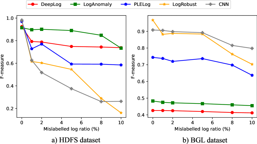
Figure 3. Results with different ratios of mislabelled logs

We can find that, on the HDFS dataset, even with just 1% of mislabelled logs, the F-measures of the studied models decline significantly. For example, LogRobust and CNN drop 37.2% and 36.2% with only 1% of noise, respectively. When the noise ratio reaches 10%, the F-measures of LogRobust and CNN drop to only 0.161 and 0.263. The results confirm that even with the advantage of semantic understanding, these DL models can lose their performance with only a small proportion of mislabelled logs. It is also true for PLELog, which leverages the semantic meaning of logs as well. Another reason for this remarkable reduction is that there are many duplicate log sequences in the HDFS dataset, thus, labeling any duplicate normal sequences as anomalies could have a large impact. Interestingly, the F-measure of LogAnomaly only drops slightly with 1% of mislabelled logs (from 0.915 to 0.897). When the mislabelled ratio is 5% and 10%, LogAnomaly can achieve better F-measures compared to other models. The reason is that LogAnomaly uses quantitative vectors to extract quantitative relationships holding in logs along with sequential vectors, thus, allowing the model to predict the possibilities of the next event more precisely.

4.4.2. The impact of log parsing errors

We also evaluate the impact of data noise introduced by log parsing errors. Log parsing errors can lead to extra log events and wrong log templates (Le and Zhang, 2021). We experiment with four commonly-used log parsers, namely Drain (He et al., 2017), Spell (Du and Li, 2016), AEL (Jiang et al., 2008), and IPLoM (Makanju et al., 2009) on all four datasets. We find that the performance of models is highly influenced by log parsers. To demonstrate our findings, we show the performance of models with different log parsers on BGL and Spirit datasets in Table 6.

Table 6. Results with different log parsers

Model		BGL				Spirit
		Drain	Spell	AEL	IPLoM	Drain	Spell	AEL	IPLoM
DeepLog	P	0.270	0.271	0.271	0.273	0.438	0.602	0.413	0.607
	R	0.988	0.988	0.988	0.988	1.0	1.0	1.0	1.0
	S	0.437	0.44	0.438	0.443	0.099	0.535	0	0.545
	F1	0.426	0.426	0.425	0.427	0.609	0.751	0.584	0.755
LogAnomaly	P	0.313	0.339	0.539	0.548	0.438	0.612	0.413	0.607
	R	0.798	0.977	0.965	0.971	1.0	1.0	1.0	1.0
	S	0.551	0.599	0.826	0.831	0.099	0.554	0	0.545
	F1	0.483	0.504	0.692	0.700	0.609	0.759	0.584	0.755
PLELog	P	0.702	0.560	0.661	0.655	0.931	0.859	0.863	0.500
	R	0.791	0.404	0.854	0.433	0.767	0.859	0.887	0.662
	S	0.899	0.938	0.907	0.952	0.690	0.901	0.901	0.535
	F1	0.744	0.476	0.744	0.521	0.841	0.859	0.875	0.570
LogRobust	P	0.994	0.849	0.844	0.726	0.985	0.947	0.986	0.973
	R	0.942	0.988	0.982	0.977	0.915	1.0	1.0	1.0
	S	0.999	0.963	0.962	0.922	0.990	0.960	0.990	0.980
	F1	0.967	0.914	0.908	0.833	0.949	0.973	0.993	0.986
CNN	P	0.871	0.994	0.942	0.937	0.986	0.959	0.986	0.986
	R	0.947	0.965	0.947	0.959	1.0	1.0	1.0	1.0
	S	0.97	0.999	0.988	0.986	0.990	0.970	0.990	0.990
	F1	0.908	0.979	0.945	0.948	0.993	0.979	0.993	0.993

We can observe that the performance of studied models varies a lot with different log parsers. For example, DeepLog achieves an F-measure of 0.755 and a Specificity of 0.545 with the IPLoM (Makanju et al., 2009) parser on Spirit dataset. When experimenting with Drain (He et al., 2017), these values drop to 0.609 and 0.099, respectively, although Drain is one of the most accurate log parsers according to a recent benchmark study (Zhu et al., 2019). The results also show that LogRobust and CNN can handle log parsing noise better than other models. This is probably because of their use of semantic vectors. Moreover, we find that different log parsing errors have distinctive impact on the detection models. The results on BGL and Spirit datasets show that DeepLog and LogAnomaly perform better with Spell (Du and Li, 2016) and IPLoM (Makanju et al., 2009) than with Drain. This is because Drain often produces many extra log events that hinder the performance of DeepLog and LogAnomaly (which use forecasting methods to predict the next log event). In contrast, other models can better handle extra log events but may fail when log parsers produce errors due to semantic misunderstanding (Le and Zhang, 2021).

4.5. RQ5: How early can the existing models detect anomalies in online detection?

To answer RQ5, we evaluate the five studied models using a fixed-window grouping of different sizes (from 20 logs to 1-hour logs). We record the number of examined log messages before each model can detect an anomaly in an online detection mode (i.e., detecting anomalies on the fly). Figure 4 uses the results with 100-logs and 0.5-hour-logs settings to explain our findings.

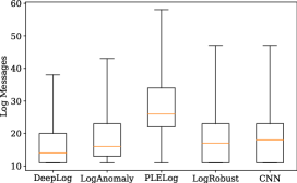
(a) Data grouping with 100 logs

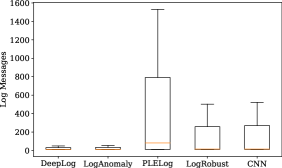
(b) Data grouping with 0.5-hour logs

Figure 4. The number of examined log messages before each model can detect an anomaly

We find that DeepLog can detect anomalies the earliest, with an average of 14.3 and 90.6 log messages with 100-logs and 0.5-hour-logs setting, respectively. LogAnomaly, which is also based on predicting the next log events, detects anomaly a bit later since it requires to capture both sequential and quantitative relationships in order to mark a log sequence as abnormal. In contrast, the use of semantic vectors could make other models, including LogRobust, CNN, and PLELog, detect anomalies much later, as shown in Figure  4. These classification-based models require to capture features of anonymous behavior to detect anomalies, thus tend to raise alarms closer to the time the anomaly happens. Figure 5 shows a case study on an anomalous log sequence (with the size of 100 logs) on BGL dataset. Five models are applied to identify whether the log sequence is abnormal or not. We find that DeepLog raises an alarm after examining 11 logs, followed by LogAnomaly, LogRobust, and CNN, while PLELog is the last model that raises an alarm (after 64 log messages arrived).

As efficiency is critical in online anomaly detection, we also evaluate the studied models by recording the time spent on both the training and testing phases. On BGL dataset, DeepLog spends 19.2 and 0.6 minutes on training and testing. LogRobust and CNN, which use higher-dimension inputs and more complex networks, consume 31.7 and 28.3 minutes on training and testing, respectively. In the testing phase, LogRobust and CNN only take 0.3 minutes. LogAnomaly, which uses two LSTM networks to learn sequential and quantitative features, spends 56.7 and 1.6 minutes on training and testing. PLELog, which contains a clustering module and a GRU module, is the most time-consuming model. Specifically, PLELog spends 36.6 minutes and 69.1 minutes to train the clustering and GRU models, respectively. In the testing phase, PLELog consumes 10.8 minutes to process the BGL dataset. The results show that PLELog may be inappropriate for online detection due to its incapability of early detection and heavy time cost.

Figure 5. Timeline for detecting an anomaly in the BGL dataset

5. Discussion

5.1. The Advantages and Disadvantages of the Studied Methods

Based on our findings, we can conclude that all the studied models do not always work as well as they claimed in their papers. Different scenarios have different impacts on the performance of anomaly detection models. We point out the advantages and disadvantages of each model as follows, which are also summarized in Table 7.

DeepLog. The main advantage of DeepLog is that it does not require any abnormal logs to build a detection model using sequential vectors, thus reducing the effort for model construction. It can also detect anomalies earlier than other models. However, due to this characteristic, DeepLog performs poorly on more complex datasets with a large number of log events (see Section 4.1). Besides, DeepLog is greatly impacted by the log parsing errors since it only leverages the index of log templates and ignores the semantic meaning of log templates (see Section 4.4.2).

LogAnomaly. LogAnomaly uses sequential and quantitative vectors to train a detection model, which can help reduce the impact of data noise caused by mislabelled logs. Like DeepLog, LogAnomaly can detect anomalies early and deal with a large amount of data since it only trains with normal logs. The main benefit of LogAnomaly is in the phase of matching similar log templates using semantic vectors. This feature allows LogAnomaly to improve the accuracy by matching new log templates with an existing one in the training logs instead of marking them as anomalies as DeepLog does. However, like DeepLog, LogAnomaly trains the model using the index of log event (sequential and quantitative vectors) and cannot learn the semantic meaning of log templates, so it is highly affected by the log parsing errors (see Section 4.4.2). Moreover, LogAnomaly cannot perform well on large datasets with a numerous log events (see Section 4.1 and 4.2).

PLELog. The main advantage of PLELog is that it can learn knowledge about historical anomalies via probabilistic label estimation. PLELog adopts a clustering method (i.e., HDBSCAN (McInnes et al., 2017)) to probabilistically estimate the labels of unlabeled log sequences. This approach allows PLELog to work with only normal logs. Besides, the use of semantic vectors and attention-based GRU network makes PLELog perform more effectively. However, PLELog is time-consuming since it requires time to train the clustering model (see Section 4.5). Moreover, PLELog cannot cope well with the noise in training data (see Section 4.4.1), and it does not perform well on the early detection task.

LogRobust. LogRobust leverages semantic vectors of log templates together with an attention-based Bi-LSTM model. LogRobust can work well with the noise from log parsing errors by utilizing the attention-based Bi-LSTM model, which has the ability to capture the contextual information of log sequences. However, as the main characteristic of supervised models, LogRobust requires both normal and abnormal data in the training phase, which would cost much manual labeling effort. Another drawback of LogRobust is that it can be greatly affected by the noise from mislabelled logs (see Section 4.4.1).

CNN. The Convolutional Neural Network can mine more relationships in log context by leveraging multiple filters. The convolution operation allows CNN to capture not only the correlation between log templates but also the correlation inside the semantic embedding of log templates (Lu et al., 2018). CNN can achieve high accuracy on many datasets using a supervised approach. However, like LogRobust, CNN requires a large amount of labeled data, which is mostly unavailable in practice. CNN also loses its accuracy when dealing with highly imbalanced data and data noise (see Sections 4.3 and 4.4.1).

Table 7. A Comparison of Different Log-based Anomaly Detection Approaches with Deep Learning

Model	Pros	Cons	Data Requirements
DeepLog	Relatively simple, only require normal data. Good at detecting anomalies early detection.	Perform poorly on complex datasets. Heavily impacted by the log parsing errors.	Normal labeled and simple data.
LogAnomaly	Only require normal data. Can match new log templates with existing ones in the training data.	Perform poorly on complex datasets. Heavily impacted by the log parsing errors.	Normal labeled and simple data.
PLELog	Only require normal and unlabelled data. Good performance compared to semi-supervised methods. Can learn the semantic meaning of log templates.	Cannot work well with the noise in training data and in the early detection task. Complex design and time-consuming.	Partially labeled data.
LogRobust	Good performance on many datasets. Can capture the contextual information of log sequences to handle log parsing errors and the instability of logs.	Require a large amount of labeled data. Heavily impacted by mislabelled logs.	Fully labeled data.
CNN	Good performance on many datasets. Can handle log parsing errors.	Require a large amount of labeled data. Heavily impacted by mislabelled logs.	Fully labeled data.

5.2. Future Research Work

Based on our findings, we identify the following research challenges and also suggest possible solutions:

A variety of datasets. Our findings suggest that more datasets should be used for a more comprehensive evaluation of log-based anomaly detection models. A good result on one dataset does not necessarily reflect good performance on other datasets due to a variety of data characteristics (e.g., class distributions, noise, etc.).

Limited labelled data. Although supervised learning-based methods (i.e., LogRobust and CNN) can achieve higher accuracy than the unsupervised counterparts, it is time-consuming and tedious to manually label the anomalies due to the volume and velocity of log data. Semi-supervised learning-based models (i.e., DeepLog, LogAnomaly, and PLELog) can deal with a large amount of data as they only require normal data. However, the accuracy achieved by existing methods is rather low in practice, as shown in Section 4.1. Improving the accuracy of semi-supervised models or designing unsupervised models is a challenging but essential future work.

Early detection. Our findings show that different models have different abilities in early detection of system anomalies. The anomalies should be predicted as early as possible to allow enough time for any preparatory or preventive actions in an online detection scenario. More work is needed to build effective models that allow sufficient lead time (i.e., reducing the number of log messages being examined) and meanwhile achieve high prediction accuracy.

Evolving systems. Our findings show that log parsing errors have impact on log-based anomaly detection. Log parsing errors can be introduced by the change of logging statements during software evolution (Zhang et al., 2019; Le and Zhang, 2021). As real-world software systems constantly evolve, new log events always appear (Zhang et al., 2019; Kabinna et al., 2018). Therefore, existing log-based anomaly detection models will either fail to work due to the incompatibility with new logs or result in low performance due to the incorrect classification. Therefore, models should be able to learn the semantic meaning of the whole log messages to handle the instability of logs of evolving systems.

Relations among log events. As discussed in Section 4.2, session window grouping gathers logs in a specific execution path, which could possess more relations among log events than the fixed-window grouping method. Existing methods convert logs into sequences, which capture sequential relationships among log messages. A possible research direction is to explore more relationships between logs, such as the logical relationships and interactive relationships among logging components (Liu et al., 2019), to capture a variety of anomalous behavior.

5.3. Threats to Validity

During our study, we have identified the following major threats to the validity.

Limited models. In this work, we only experimentally evaluate five representative models that have publicly available source code. In the future, we will aim to re-implement the DL models that did not release their source code based on the descriptions in their papers and then perform a larger-scale evaluation.

Reimplementation. We mainly adopt the public implementations of studied models. For LogRobust, as its original implementation is based on Keras, we convert it into a PyTorch-based implementation so that we have a unified framework for all log-based anomaly detection tools. In our version, we use the same hyperparameters that are provided by the authors of LogRobust. For LogAnomaly and CNN, we use the FastText model to replace the missing semantic embedding components from public implementations. To reduce this threat, we experiment on the same settings and datasets from the original paper and confirm that our results are similar with the reported values.

Limited datasets. Our experiments are conducted on four public log datasets. Although they are widely used in existing studies on log-based anomaly detection, they may not represent all characteristics of log data. To overcome this threat, we create synthetic datasets for evaluating models with different data characteristics (e.g., different class distributions and different labeling noise). In the future, we will experiment on more datasets, including industrial datasets, to cover more real-world scenarios.

Data quality. Our experiments are conducted based on four datasets that are manually inspected and labeled by engineers. However, our experiment on data noises shows that a small portion of mislabelled logs could downgrade the performance of anomaly detection models. To reduce this threat, we experiment with four public datasets. We also create synthetic datasets by injecting a specific portion of mislabelled logs. In our future work, we will explore methods for measuring and improving the quality of datasets.

6. Conclusion

We have conducted an in-depth analysis of recent deep learning models for log-based anomaly detection. We have investigated several aspects of model evaluation: training data selection strategies, different characteristics of datasets, and early detection capability. Our results point out that all these aspects have large impact on the evaluation results and the performance of the models is often not as good as expected. Our findings show that the problem of log-based anomaly detection has not been solved yet. We also suggest some possible future work. We hope that the results and findings of our study can be of great help for practitioners and researchers working on this interesting area.

Our source code and detailed experimental data are available at https://github.com/LogIntelligence/LogADEmpirical. The datasets including the synthetic data that is used for evaluating models with different data characteristics, can also serve as a benchmark for evaluating future log-based anomaly detection models.

- (1)
- ple (2021) 2021. Implementation of PLELog. Retrieved August 27, 2021 from https://github.com/YangLin-George/PLELog
- log (2021a) 2021a. A large collection of system log datasets for AI-powered log analytics. Retrieved August 31, 2021 from https://github.com/logpai/loghub
- don (2021) 2021. Log Anomaly Detection Toolkit. Retrieved August 27, 2021 from https://github.com/donglee-afar/logdeep
- wuy (2021) 2021. A Pytorch implementation of DeepLog. Retrieved August 21, 2021 from https://github.com/wuyifan18/DeepLog
- log (2021b) 2021b. A toolkit for automated log parsing. Retrieved August 31, 2021 from https://github.com/logpai/logparser
- Breier and Branišová (2015) Jakub Breier and Jana Branišová. 2015. Anomaly detection from log files using data mining techniques. In Information Science and Applications. Springer, 449–457.
- Chen et al. (2004) Mike Chen, Alice X Zheng, Jim Lloyd, Michael I Jordan, and Eric Brewer. 2004. Failure diagnosis using decision trees. In International Conference on Autonomic Computing, 2004. Proceedings. IEEE, 36–43.
- Chen et al. (2021) Zhuangbin Chen, Jinyang Liu, Wenwei Gu, Yuxin Su, and Michael R Lyu. 2021. Experience Report: Deep Learning-based System Log Analysis for Anomaly Detection. arXiv preprint arXiv:2107.05908 (2021).
- Cho et al. (2014) Kyunghyun Cho, Bart Van Merriënboer, Caglar Gulcehre, Dzmitry Bahdanau, Fethi Bougares, Holger Schwenk, and Yoshua Bengio. 2014. Learning phrase representations using RNN encoder-decoder for statistical machine translation. arXiv preprint arXiv:1406.1078 (2014).
- Dai et al. (2020) Hetong Dai, Heng Li, Che Shao Chen, Weiyi Shang, and Tse-Hsun Chen. 2020. Logram: Efficient log parsing using n-gram dictionaries. IEEE Transactions on Software Engineering (2020).
- Du and Li (2016) Min Du and Feifei Li. 2016. Spell: Streaming parsing of system event logs. In 2016 IEEE 16th International Conference on Data Mining (ICDM). IEEE, 859–864.
- Du et al. (2017) Min Du, Feifei Li, Guineng Zheng, and Vivek Srikumar. 2017. Deeplog: Anomaly detection and diagnosis from system logs through deep learning. In Proceedings of the 2017 ACM SIGSAC Conference on Computer and Communications Security. 1285–1298.
- Farzad and Gulliver (2020) Amir Farzad and T Aaron Gulliver. 2020. Unsupervised log message anomaly detection. ICT Express 6, 3 (2020), 229–237.
- Fenton and Ohlsson (2000) Norman E. Fenton and Niclas Ohlsson. 2000. Quantitative analysis of faults and failures in a complex software system. IEEE Transactions on Software engineering 26, 8 (2000), 797–814.
- Guo et al. (2021) Haixuan Guo, Shuhan Yuan, and Xintao Wu. 2021. LogBERT: Log Anomaly Detection via BERT. arXiv preprint arXiv:2103.04475 (2021).
- Hamooni et al. (2016) Hossein Hamooni, Biplob Debnath, Jianwu Xu, Hui Zhang, Guofei Jiang, and Abdullah Mueen. 2016. Logmine: Fast pattern recognition for log analytics. In Proceedings of the 25th ACM International on Conference on Information and Knowledge Management. 1573–1582.
- He et al. (2017) Pinjia He, Jieming Zhu, Zibin Zheng, and Michael R Lyu. 2017. Drain: An online log parsing approach with fixed depth tree. In 2017 IEEE International Conference on Web Services (ICWS). IEEE, 33–40.
- He et al. (2020a) Shilin He, Pinjia He, Zhuangbin Chen, Tianyi Yang, Yuxin Su, and Michael R Lyu. 2020a. A Survey on Automated Log Analysis for Reliability Engineering. arXiv preprint arXiv:2009.07237 (2020).
- He et al. (2016) Shilin He, Jieming Zhu, Pinjia He, and Michael R Lyu. 2016. Experience report: System log analysis for anomaly detection. In ISSRE 2016. IEEE, 207–218.
- He et al. (2020b) Shilin He, Jieming Zhu, Pinjia He, and Michael R Lyu. 2020b. Loghub: a large collection of system log datasets towards automated log analytics. arXiv preprint arXiv:2008.06448 (2020).
- Hochreiter and Schmidhuber (1997) Sepp Hochreiter and Jürgen Schmidhuber. 1997. Long short-term memory. Neural computation 9, 8 (1997), 1735–1780.
- Jiang et al. (2008) Zhen Ming Jiang, Ahmed E Hassan, Parminder Flora, and Gilbert Hamann. 2008. Abstracting execution logs to execution events for enterprise applications (short paper). In 2008 The Eighth International Conference on Quality Software. IEEE, 181–186.
- Joulin et al. (2016) Armand Joulin, Edouard Grave, Piotr Bojanowski, Matthijs Douze, Hérve Jégou, and Tomas Mikolov. 2016. Fasttext. zip: Compressing text classification models. arXiv preprint arXiv:1612.03651 (2016).
- Kabinna et al. (2018) Suhas Kabinna, Cor-Paul Bezemer, Weiyi Shang, Mark D Syer, and Ahmed E Hassan. 2018. Examining the stability of logging statements. Empirical Software Engineering 23, 1 (2018), 290–333.
- Kim (2014) Yoon Kim. 2014. Convolutional Neural Networks for Sentence Classification. In Proceedings of the 2014 Conference on Empirical Methods in Natural Language Processing (EMNLP). Association for Computational Linguistics, Doha, Qatar.
- Le and Zhang (2021) Van-Hoang Le and Hongyu Zhang. 2021. Log-based Anomaly Detection Without Log Parsing. In 2021 36th IEEE/ACM International Conference on Automated Software Engineering (ASE). 492–504.
- Li et al. (2020) Xiaoyun Li, Pengfei Chen, Linxiao Jing, Zilong He, and Guangba Yu. 2020. SwissLog: Robust and Unified Deep Learning Based Log Anomaly Detection for Diverse Faults. In ISSRE 2020. IEEE, 92–103.
- Lin et al. (2018) Qingwei Lin, Ken Hsieh, Yingnong Dang, Hongyu Zhang, Kaixin Sui, Yong Xu, Jian-Guang Lou, Chenggang Li, Youjiang Wu, Randolph Yao, et al. 2018. Predicting node failure in cloud service systems. In ESEC/FSE 2018. 480–490.
- Lin et al. (2016) Qingwei Lin, Hongyu Zhang, Jian-Guang Lou, Yu Zhang, and Xuewei Chen. 2016. Log Clustering Based Problem Identification for Online Service Systems. In Proceedings of the 38th International Conference on Software Engineering Companion (Austin, Texas) (ICSE ’16). 102–111.
- Liu et al. (2019) Fucheng Liu, Yu Wen, Dongxue Zhang, Xihe Jiang, Xinyu Xing, and Dan Meng. 2019. Log2vec: A heterogeneous graph embedding based approach for detecting cyber threats within enterprise. In Proceedings of the 2019 ACM SIGSAC Conference on Computer and Communications Security. 1777–1794.
- Liu et al. (2021) Xu Liu, Weiyou Liu, Xiaoqiang Di, Jinqing Li, Binbin Cai, Weiwu Ren, and Huamin Yang. 2021. LogNADS: Network anomaly detection scheme based on semantic representation. Future Generation Computer Systems (2021).
- Lou et al. (2010) Jian-Guang Lou, Qiang Fu, Shengqi Yang, Ye Xu, and Jiang Li. 2010. Mining Invariants from Console Logs for System Problem Detection.. In USENIX Annual Technical Conference. 1–14.
- Lu et al. (2018) Siyang Lu, Xiang Wei, Yandong Li, and Liqiang Wang. 2018. Detecting anomaly in big data system logs using convolutional neural network. In 2018 IEEE 16th Intl Conf on Dependable, Autonomic and Secure Computing, 16th Intl Conf on Pervasive Intelligence and Computing, 4th Intl Conf on Big Data Intelligence and Computing and Cyber Science and Technology Congress (DASC/PiCom/DataCom/CyberSciTech). IEEE, 151–158.
- Makanju et al. (2009) Adetokunbo AO Makanju, A Nur Zincir-Heywood, and Evangelos E Milios. 2009. Clustering event logs using iterative partitioning. In Proceedings of the 15th ACM SIGKDD international conference on Knowledge discovery and data mining. 1255–1264.
- McInnes et al. (2017) Leland McInnes, John Healy, and Steve Astels. 2017. hdbscan: Hierarchical density based clustering. Journal of Open Source Software 2, 11 (2017), 205.
- Meng et al. (2019) Weibin Meng, Ying Liu, Yichen Zhu, Shenglin Zhang, Dan Pei, Yuqing Liu, Yihao Chen, Ruizhi Zhang, Shimin Tao, Pei Sun, et al. 2019. LogAnomaly: Unsupervised Detection of Sequential and Quantitative Anomalies in Unstructured Logs.. In IJCAI, Vol. 7. 4739–4745.
- Mi et al. (2013) Haibo Mi, Huaimin Wang, Yangfan Zhou, Michael Rung-Tsong Lyu, and Hua Cai. 2013. Toward fine-grained, unsupervised, scalable performance diagnosis for production cloud computing systems. IEEE Transactions on Parallel and Distributed Systems 24, 6 (2013), 1245–1255.
- Nagappan and Vouk (2010) Meiyappan Nagappan and Mladen A Vouk. 2010. Abstracting log lines to log event types for mining software system logs. In 2010 7th IEEE Working Conference on Mining Software Repositories (MSR 2010). IEEE, 114–117.
- Nedelkoski et al. (2020) Sasho Nedelkoski, Jasmin Bogatinovski, Alexander Acker, Jorge Cardoso, and Odej Kao. 2020. Self-attentive classification-based anomaly detection in unstructured logs. arXiv preprint arXiv:2008.09340 (2020).
- Oliner and Stearley (2007) Adam Oliner and Jon Stearley. 2007. What supercomputers say: A study of five system logs. In DSN 2007. IEEE, 575–584.
- Pennington et al. (2014) Jeffrey Pennington, Richard Socher, and Christopher D Manning. 2014. Glove: Global vectors for word representation. In Proceedings of the 2014 conference on empirical methods in natural language processing (EMNLP). 1532–1543.
- Shima (2016) Keiichi Shima. 2016. Length matters: Clustering system log messages using length of words. arXiv preprint arXiv:1611.03213 (2016).
- Sokolova et al. (2006) Marina Sokolova, Nathalie Japkowicz, and Stan Szpakowicz. 2006. Beyond accuracy, F-score and ROC: a family of discriminant measures for performance evaluation. In Australasian joint conference on artificial intelligence. Springer, 1015–1021.
- Tang et al. (2011) Liang Tang, Tao Li, and Chang-Shing Perng. 2011. LogSig: Generating system events from raw textual logs. In Proceedings of the 20th ACM international conference on Information and knowledge management. 785–794.
- Vaarandi and Pihelgas (2015) Risto Vaarandi and Mauno Pihelgas. 2015. Logcluster-a data clustering and pattern mining algorithm for event logs. In 2015 11th International conference on network and service management (CNSM). IEEE, 1–7.
- Vaswani et al. (2017) Ashish Vaswani, Noam Shazeer, Niki Parmar, Jakob Uszkoreit, Llion Jones, Aidan N Gomez, Lukasz Kaiser, and Illia Polosukhin. 2017. Attention is all you need. arXiv preprint arXiv:1706.03762 (2017).
- Xu et al. (2009) Wei Xu, Ling Huang, Armando Fox, David Patterson, and Michael I Jordan. 2009. Detecting large-scale system problems by mining console logs. In Proceedings of the ACM SIGOPS 22nd symposium on Operating systems principles. 117–132.
- Yang et al. (2021) Lin Yang, Junjie Chen, Zan Wang, Weijing Wang, Jiajun Jiang, Xuyuan Dong, and Wenbin Zhang. 2021. Semi-supervised log-based anomaly detection via probabilistic label estimation. In ICSE 2021. IEEE, 1448–1460.
- Yerushalmy (1947) Jacob Yerushalmy. 1947. Statistical problems in assessing methods of medical diagnosis, with special reference to X-ray techniques. Public Health Reports (1896-1970) (1947), 1432–1449.
- Zhang et al. (2020) Bo Zhang, Hongyu Zhang, Pablo Moscato, and Aozhong Zhang. 2020. Anomaly Detection via Mining Numerical Workflow Relations from Logs. In 2020 International Symposium on Reliable Distributed Systems (SRDS). IEEE, 195–204.
- Zhang (2008) Hongyu Zhang. 2008. On the distribution of software faults. IEEE Transactions on Software Engineering 34, 2 (2008), 301–302.
- Zhang (2009) Hongyu Zhang. 2009. An investigation of the relationships between lines of code and defects. In 2009 IEEE International Conference on Software Maintenance. IEEE, 274–283.
- Zhang and Zhang (2007) Hongyu Zhang and Xiuzhen Zhang. 2007. Comments on” data mining static code attributes to learn defect predictors”. IEEE Transactions on Software Engineering 33, 9 (2007), 635–637.
- Zhang et al. (2019) Xu Zhang, Yong Xu, Qingwei Lin, Bo Qiao, Hongyu Zhang, Yingnong Dang, Chunyu Xie, Xinsheng Yang, Qian Cheng, Ze Li, et al. 2019. Robust log-based anomaly detection on unstable log data. In ESEC/FSE 2019. 807–817.
- Zhu et al. (2019) Jieming Zhu, Shilin He, Jinyang Liu, Pinjia He, Qi Xie, Zibin Zheng, and Michael R Lyu. 2019. Tools and benchmarks for automated log parsing. In ICSE 2019. IEEE, 121–130.