Yang, Zhong, and Tan

Optimal Clustering with Bandit Feedback

Optimal Clustering with Bandit Feedback

Junwen Yang Institute of Operations Research and Analytics, National University of Singapore, Singapore 117602, junwen_yang@u.nus.edu Zixin Zhong Department of Electrical and Computer Engineering, National University of Singapore, Singapore 117583,
Department of Mathematics, National University of Singapore, Singapore 119076, zixin.zhong@u.nus.edu Vincent Y. F. Tan Department of Mathematics, National University of Singapore, Singapore 119076,
Department of Electrical and Computer Engineering, National University of Singapore, Singapore 117583,
Institute of Operations Research and Analytics, National University of Singapore, Singapore 117602, vtan@nus.edu.sg

This paper considers the problem of online clustering with bandit feedback. A set of arms (or items) can be partitioned into various groups that are unknown. Within each group, the observations associated to each of the arms follow the same distribution with the same mean vector. At each time step, the agent queries or pulls an arm and obtains an independent observation from the distribution it is associated to. Subsequent pulls depend on previous ones as well as the previously obtained samples. The agent’s task is to uncover the underlying partition of the arms with the least number of arm pulls and with a probability of error not exceeding a prescribed constant $\delta$. The problem proposed finds numerous applications from clustering of variants of viruses to online market segmentation. We present an instance-dependent information-theoretic lower bound on the expected sample complexity for this task, and design a computationally efficient and asymptotically optimal algorithm, namely Bandit Online Clustering (BOC). The algorithm includes a novel stopping rule for adaptive sequential testing that circumvents the need to exactly solve any NP-hard weighted clustering problem as its subroutines. We show through extensive simulations on synthetic and real-world datasets that BOC’s performance matches the lower bound asymptotically, and significantly outperforms a non-adaptive baseline algorithm.

clustering, $K$-means, online learning, multi-armed bandits, pure exploration

1 Introduction

Clustering, the task of partitioning a set of items into smaller clusters based on their commonalities, is one of the most fundamental tasks in data analysis and machine learning with a rich and diverse history (Driver and Kroeber 1932, Cattell 1943, Ruspini 1969, Jain et al. 1999, Celebi et al. 2013). It has numerous applications in a wide variety of areas including business analytics, bioinformatics, pattern recognition, and social sciences. In this era of abundance of medical data, clustering is a powerful tool to uncover the underlying patterns of unknown treatments or diseases when related systematic knowledge is underdeveloped (MacCuish and MacCuish 2010). In commercial decision making, aiming at increasing customer satisfaction and maximizing potential benefit, marketers utilize clustering strategies to partition the inclusive business market into more narrow market segments with similar characteristics (Chaturvedi et al. 1997). Due to its enormous importance in practical applications, clustering has been studied extensively in the literature from multidisciplinary perspectives. A plethora of algorithms (e.g., $K$-means and spectral clustering) have been proposed for the task of clustering (see Jain et al. (1999) or Saxena et al. (2017) for comprehensive reviews). In particular, the $K$-means algorithm by MacQueen (1967) and Lloyd (1982) is arguably the most ubiquitous algorithm due to its simplicity, efficiency, and empirical successes (Jain 2010).

Although modern data analysis has benefited immensely from the abundance and richness of data, there is an urgent need to develop new techniques that are adapted to the sequential and uncertain nature of data collection. In this paper, we are interested in online clustering with bandit feedback, which is an online variant of the classical offline clustering problem. With bandit feedback, the agent only observes a noisy measurement on the selected arm (or item) at each time step. However, the agent can decide which arm to pull adaptively, so as to minimize the expected number of total arm pulls it takes to correctly partition the given arm set with a given (high) probability.

Two Motivating Examples. Our online clustering model captures various contemporary real-world scenarios, in which data contaminated by some degree of measurement noise become available in a sequential and adaptive fashion. We are firstly motivated by medical and public health professionals’ arduous battles against new viruses (e.g., COVID-19). In the face of an unknown type of virus that has different variants, let us assume that there is only one dominant variant in each sub-region of a particular state. When accurate laboratory analysis is not available especially in underdeveloped regions, how can healthcare professionals partition the virus samples into specific dominant variants based on noisy measurements of infectious patients from various sub-regions? This realistic and critical problem can be well modelled by our framework, namely online clustering with bandit feedback, where the healthcare personnel adaptively obtains independent observations of patients from the selected sub-regions and finally partitions the whole state into various groups based on the types of dominant variants. Due to the prohibitive costs in obtaining the measurements, this must be done with as few of them as possible.

\begin{overpic}[width=433.62pt]{figs/clustering-Page-4-v4.pdf} \put(83.7,42.0){Time} \put(14.0,42.0){$1$} \put(19.3,42.0){$2$} \put(24.6,42.0){$3$} \put(29.9,42.0){$4$} \put(35.2,42.0){$5$} \put(40.5,42.0){$6$} \put(45.8,42.0){$7$} \put(51.1,42.0){$8$} \put(56.4,42.0){$9$} \put(61.1,42.0){$10$} \put(66.4,42.0){$11$} \put(71.7,42.0){$12$} \end{overpic}

Example involving partitioning $6$ sub-groups of customers into $3$ market segments with bandit feedback. Customers are divided into sub-groups based on some basic characteristics (e.g., age and gender). At each point in time, an algorithm chooses which sub-group to query and receives a multidimensional sample (e.g., ratings of a set of products) from one customer of that sub-group. Based on the previously chosen sub-groups and their samples, the algorithm decides which sub-group to query next. Finally, when it is sufficiently confident of producing a partition of the sub-groups into market segments that share similar preferences, the algorithm terminates.

Our second motivation is in digital marketing in which customer feedback on certain products are collected in an online manner and always accompanied by random or systematic noise. For market segmentation, one important objective is to reduce the cost of feedback collection while maintaining a high quality of clustering, so that subsequent recommendations are suitably tailored to particular groups of consumers. See Figure 1 for a protocol of online market segmentation that our framework is able to model well.

Main Contributions. Our main contributions are as follows:

1. We formulate the online clustering with bandit feedback problem in Section 3. We identify some subtleties of the framework, which may be of independent interest for future research. In particular, there are multiple ways that a partition of an arm set can be represented. This is further complicated by the fact that each cluster is also identified by a mean vector. We propose a precise expression for an instance of cluster bandits, and establish two equivalence relations for the partitions and bandit instances, respectively.

2. In Section 4, we derive an instance-dependent (information-theoretic) lower bound on the expected sample complexity for the online clustering problem; this lower bound, however, involves a tricky optimization problem. By exploiting the structure of the problem and leveraging an interesting combinatorial property, we simplify the optimization to a finite convex minimax problem, which can be solved efficiently. Further analyses of the lower bound provide fundamental insights and essential tools for the design of our algorithm.

3. In Section 5, we propose and analyze Bandit Online Clustering (or BOC). We show that it is not only computationally efficient but also asymptotically optimal in the sense that its expected sample complexity attains the lower bound as the error probability tends to zero. This result is somewhat surprising since solving the corresponding offline clustering problem exactly is NP-hard (Aloise et al. 2009, Mahajan et al. 2012). En route to overcoming this combinatorial challenge and demonstrating desirable properties of BOC, we utilize a variant of the classical $K$-means algorithm in the sampling rule and propose a novel stopping rule for adaptive sequential testing. In particular, the “natural” stopping rule based on the generalized likelihood ratio (GLR) statistic (Chernoff 1959, Garivier and Kaufmann 2016) is intractable. Our workaround involves another statistic that exploits our insights on the lower bound. Finally in Section 6, we show via numerical experiments that BOC is indeed asymptotically optimal and significantly outperforms a uniform sampling strategy on both synthetic and real-world benchmark datasets.

2 Literature Review

Clustering and the $K$-means algorithm. Although we consider an online version of the clustering problem, a certain variant of the classical (offline) $K$-means algorithm serves as a subroutine of BOC. Given the $d$-dimensional observations of $M$ items, the $K$-means algorithm (MacQueen 1967, Lloyd 1982) aims at partitioning the items into $K$ disjoint clusters in order to minimize the sum of squared Euclidean distances between each item to the center of its associated cluster. If each item is associated to a certain weight, then a reasonable objective is the minimization of the weighted sum of squared Euclidean distances. Due to the prominence of the $K$-means algorithm, the corresponding clustering problem is also referred to as the (weighted) $K$-means clustering problem in the literature. This non-convex $K$-means clustering problem has been shown to be NP-hard even for $d=2$ (Mahajan et al. 2012) or $K=2$ (Aloise et al. 2009). In fact, for general $d$, $K$ and $M$, the problem can be exactly solved in $O(M^{dK+1})$ time (Inaba et al. 1994). When used as a heuristic algorithm, the performance of $K$-means depends to a large extent on how it is initialized. To improve the stability and the quality of the eventual solution that $K$-means produces, various initialization methods have been proposed (e.g., Forgy’s method (Forgy 1965), Maximin (Gonzalez 1985), $K$-means++ (Arthur and Vassilvitskii 2007), PCA-Part (Su and Dy 2007)). See Celebi et al. (2013) for detailed comparisons on initialization methods for $K$-means.

There have been some attempts in the literature to adapt the vanilla $K$-means algorithm to an online framework involving streams of incoming data (Choromanska and Monteleoni 2012, Liberty et al. 2016, Cohen-Addad et al. 2021). In this line of works, each item only has one observation. In particular, at each time step $t$, the agent receives an observation of one item and has to determine its cluster index before the arrival of next observation. This is vastly different from our setting of bandit feedback, where the arm pulls are determined adaptively by the agent and the observations are stochastic. In addition, another related work by Khaleghi et al. (2012) addressed the case where every item is associated with an infinite sequence generated by one of $K$ unknown stationary ergodic processes. At each time step $t$, some observations arrive, each being either a new sequence or the continuation of some previously observed sequence, and the agent needs to partition the observed sequences into $K$ groups. To the best of our knowledge, the online clustering with bandit feedback problem (formally described in Section 3) has not been considered before.

Bandit Algorithms. The stochastic multi-armed bandit problem, originally introduced by Thompson (1933), provides a simple but powerful online learning framework. This problem has been studied extensively in recent years. While the regret minimization problem aims at maximizing the cumulative reward by balancing the trade-off between exploration and exploitation (Auer et al. 2002, Abbasi-Yadkori et al. 2011, Bubeck and Cesa-Bianchi 2012, Agrawal and Goyal 2012), the pure exploration problem focuses on efficient exploration with specific goals, e.g., best (top-$k$) arm identification (Even-Dar et al. 2006, Audibert et al. 2010, Karnin et al. 2013, Garivier and Kaufmann 2016, Jun et al. 2016), and its variants in linear bandits (Soare et al. 2014, Jedra and Proutiere 2020, Yang and Tan 2021), and cascading bandits (Zhong et al. 2020), among others. Our online clustering task can also be viewed as a pure exploration problem although the rewards are multi-dimensional and the arm set has an inherent cluster structure. It is worth mentioning that Prabhu et al. (2020) introduced a framework of sequential multi-hypothesis testing with bandit feedback, which is a generalization of the odd arm identification problem (Vaidhiyan and Sundaresan 2017). Our online clustering problem falls within this framework if each partition of the arm set is viewed as a hypothesis. However, the methodology proposed in Prabhu et al. (2020) relies heavily on a strong continuity assumption on the proportions of arm pulls (Assumption A therein). Even if one accepts continuity assumption, the total number of hypotheses (i.e., the number of possible partitions) is prohibitively large and the corresponding computation of the modified GLR is intractable (see Remark 5.8 for more details). Our work does away with the continuity assumption and, in fact, proves that the required continuity property holds (see Proposition 4.7). We refer to Lattimore and Szepesvári (2020) for a comprehensive review on bandit algorithms.

There is also a line of works that incorporates cluster structures into multi-armed bandits. In particular, Nguyen and Lauw (2014), Gentile et al. (2014), Li et al. (2016), and Carlsson et al. (2021) assume that users can be divided into groups and the users within each group receive similar rewards for each arm. Besides, Bouneffouf et al. (2019) and Singh et al. (2020) assume that the arm set is pre-clustered and the reward distributions of the arms within each cluster are similar. However, all the works mentioned above focus on leveraging the cluster structure to improve the performance of regret minimization, which differs from our objective, i.e., to uncover the underlying partition of the arms. Finally, Wang and Scarlett (2022) considered a min-max grouped bandits problem in which the objective is to find a sub-group (among possibly overlapping groups) whose worst arm has the highest mean reward.

3 Problem Setup and Preliminaries

A Bandit Feedback Model with Cluster Structure. We consider a bandit feedback model, in which the arm set has an inherent cluster structure. In particular, the agent is given an arm set $\mathcal{A}=[M]$, which can be partitioned into $K$ disjoint nonempty clusters, and the arms in the same cluster share the same $d$-dimensional mean vector, also referred to as the center of the corresponding cluster. Without loss of generality, we assume that $K<M$, otherwise there is only one possible partition. Therefore, an instance of cluster bandits can be fully characterized by a pair $(c,\mathcal{U})$, where $c=[c_{1},c_{2},\ldots,c_{M}]\in[K]^{M}$ consists of the cluster indices of the arms and $\mathcal{U}=[\mu(1),\mu(2),\ldots,\mu(K)]\in\mathbb{R}^{d\times K}$ represents the $K$ centers of the clusters. Since each cluster has at least one arm, for any cluster $k\in[K]$, there exists an arm $m\in[M]$ such that $c_{m}=k$. To reduce clutter and ease the reading, we always index the arms and the clusters by subscripts and numbers in parentheses, respectively.

\begin{overpic}[width=346.89731pt]{figs/model.pdf} \put(7.0,46.0){$\{m\in[M]:c_{m}=1\}$} \put(34.0,46.0){$\{m\in[M]:c_{m}=2\}$} \put(66.0,46.0){$\{m\in[M]:c_{m}=3\}$} \put(-12.0,33.0){Arm set $[M]$:} \put(9.0,33.0){$1$} \put(16.0,33.0){$2$} \put(23.0,33.0){$3$} \put(30.5,33.0){$4$} \put(39.0,33.0){$5$} \put(47.0,33.0){$6$} \put(56.0,33.0){$7$} \put(64.0,33.0){$8$} \put(72.0,33.0){$9$} \put(79.0,33.0){$10$} \put(86.0,33.0){$11$} \put(94.0,33.0){$12$} \put(-12.0,24.0){Mean vectors:} \put(18.0,24.0){$\mu(1)$} \put(42.0,24.0){$\mu(2)$} \put(72.0,24.0){$\mu(3)$} \put(0.0,10.0){If $A_{t}=2$, then $X_{t}=\mu(c_{2})+\eta_{t}$.} \put(46.0,10.0){If $A_{t+1}=8$, then $X_{t+1}=\mu(c_{8})+\eta_{t+1}$.} \end{overpic}

Online clustering with bandit feedback with $K=3$ and $M=12$.

At each time $t$, the agent selects an arm $A_{t}$ from the arm set $\mathcal{A}$, and then observes an noisy measurement on the mean vector of $A_{t}$, i.e.,

$$X_{t}=\mu(c_{A_{t}})+\eta_{t}$$

where $\{\eta_{t}\}_{t=1}^{\infty}\subset\mathbb{R}^{d}$ is a sequence of independent (noise) random variables, each following the standard $d$-dimensional Gaussian distribution $\mathcal{N}(\mathbf{0},\mathbf{I}_{d}).$ See Figure 3 for a schematic of the model.

The Equivalences of Partitions and Instances. The representation of a partition $c$ or an instance $(c,\mathcal{U})$ is not unique and we can accordingly define two equivalence relations. For a permutation $\sigma$ on $[K]$, let $\sigma(c):=[\sigma(c_{1}),\sigma(c_{2}),\ldots,\sigma(c_{M})]$ and $\sigma(\mathcal{U}):=[\mu(\sigma(1)),\mu(\sigma(2)),\ldots,\mu(\sigma(K))]$. Similarly, we define $\sigma(c,\mathcal{U}):=(\sigma(c),\sigma(\mathcal{U}))$.

For two partitions $c$ and $c^{\prime}$, if there exists a permutation $\sigma$ on $[K]$ such that $c=\sigma(c^{\prime})$, then we write $c\sim c^{\prime}$. Due to the bijectivity of permutations, there also exists another permutation $\sigma^{-1}$ on $[K]$ such that $c^{\prime}=\sigma^{-1}(c)$. Therefore, it is straightforward to verify this is indeed an equivalence relation.

For two instances $(c,\mathcal{U})$ and $(c^{\prime},\mathcal{U}^{\prime})$, if $\mu(c_{m})=\mu^{\prime}(c^{\prime}_{m})$ for all $m\in[M]$, then the two instances are equivalent and we denote this as $(c,\mathcal{U})\sim(c^{\prime},\mathcal{U}^{\prime})$. Note that $(c^{\prime},\mathcal{U}^{\prime})=\sigma(c,\mathcal{U})$ for some permutation $\sigma$ indicates $(c,\mathcal{U})\sim(c^{\prime},\mathcal{U}^{\prime})$, but the reverse implication may not be true. That is to say, if $(c,\mathcal{U})\sim(c^{\prime},\mathcal{U}^{\prime})$, there may not exist a permutation $\sigma$ such that $(c^{\prime},\mathcal{U}^{\prime})=\sigma(c,\mathcal{U})$. See Example 3.1.

Example 3.1

Let $K=2$, $M=3$ and $d=1$. Consider the three instances $(c,\mathcal{U})$, $(c^{\prime},\mathcal{U}^{\prime})$ and $(c^{\prime\prime},\mathcal{U}^{\prime\prime})$ where $c=[1,1,2]$ , $c^{\prime}=[2,2,1]$, $c^{\prime\prime}=[1,2,2]$ and $\mathcal{U}=\mathcal{U}^{\prime}=\mathcal{U}^{\prime\prime}=[1,1]$. Although $(c,\mathcal{U})\sim(c^{\prime},\mathcal{U}^{\prime})\sim(c^{\prime\prime},\mathcal{U}^{\prime\prime})$, it holds that $c\sim c^{\prime}\not\sim c^{\prime\prime}$.

Online Clustering with Bandit Feedback. We consider a pure exploration task, aiming to find the unknown cluster structure $c$ by pulling arms adaptively. In the fixed-confidence setting where a confidence level $\delta\in(0,1)$ is given, the agent is required to find a correct partition $c^{\mathrm{out}}$ of the arm set $[M]$ (i.e., $c^{\mathrm{out}}\sim c$) with a probability of at least $1-\delta$ in the smallest number of time steps.

More formally, the agent uses an online algorithm $\pi$ to decide the arm $A_{t}$ to pull at each time step $t$, to choose a time $\tau_{\delta}$ to stop pulling arms, and to recommend $c^{\mathrm{out}}$ as the partition to output eventually. Let $\mathcal{F}_{t}=\sigma(A_{1},X_{1},\ldots,A_{t},X_{t})$ denote the $\sigma$-field generated by the past measurements up to and including time $t$. Thus, the online algorithm $\pi$ consists of three components, namely,

• the sampling rule selects $A_{t}$, which is $\mathcal{F}_{t-1}$-measurable;

• the stopping rule determines a stopping time $\tau_{\delta}$ adapted to the filtration $(\mathcal{F}_{t})_{t=1}^{\infty}$;

• the recommendation rule outputs a partition $c^{\mathrm{out}}$, which is $\mathcal{F}_{\tau_{\delta}}$-measurable.

Definition 3.2

For a fixed confidence level $\delta\in(0,1)$, an online clustering algorithm $\pi$ is said to be $\delta$-PAC (probably approximately correct) if for all instances $(c,\mathcal{U})$, $\Pr(\tau_{\delta}<\infty)=1$ and the probability of error $\Pr(c^{\mathrm{out}}\not\sim c)\leq\delta$.

Our overarching goal is to design a computationally efficient online $\delta$-PAC clustering algorithm while minimizing the expected sample complexity $\operatorname{\mathbb{E}}[\tau_{\delta}]$. To rule out pathological cases that might lead to infinite expected sample complexities for any algorithm, throughout this work, we only consider partitioning the instances $(c,\mathcal{U})$ that satisfy the following natural property: the mean vectors for different clusters are distinct (i.e., the instances $(c,\mathcal{U})$ subject to $\mathcal{U}\in\mathscr{U}:=\{\bar{\mathcal{U}}\in\mathbb{R}^{d\times K}:\bar{\mu}(k_{1})\neq\bar{\mu}(k_{2})\text{ for all }1\leq k_{1}<k_{2}\leq K\}$). However, this property might not hold for general instances of cluster bandits (including the alternative instances $\mathrm{Alt}(c)$ that we introduce in the next section). Note that the odd arm identification problem (Vaidhiyan and Sundaresan 2017, Karthik and Sundaresan 2020, 2021)) is not a special case of our online clustering problem with $K=2$ since we do not require the knowledge of the number of arms in each cluster.

Other Notations. Let $\mathbb{N}$ denote the set of positive integers and $\mathbb{R}^{+}$ denote the set of non-negative real numbers. For any positive integer $N$, $\mathcal{P}_{N}:=\{x\in[0,1]^{N}:\|x\|_{1}=1\}$ denotes the probability simplex in $\mathbb{R}^{N}$ while $\mathcal{P}_{N}^{+}:=\{x\in(0,1)^{N}:\|x\|_{1}=1\}$ denotes the open probability simplex in $\mathbb{R}^{N}$.

For two partitions $c$ and $c^{\prime}$, let $d_{\mathrm{H}}(c,c^{\prime})$ denote the Hamming distance between $c$ and $c^{\prime}$, i.e., $d_{\mathrm{H}}(c,c^{\prime}):=\sum_{m=1}^{M}\mathbbm{1}\{c_{m}\neq c^{\prime}_{m}\}$. For any $a,b\in(0,1)$, the binary relative entropy, which is the KL-divergence between Bernoulli distributions with means $a$ and $b$, is denoted as $d_{\mathrm{KL}}(a,b):=a\log(a/b)+(1-a)\log((1-a)/(1-b))$.

When we write $i^{*}=\argmin_{i\in A}f(i)$ where $f(i)$ is a function of $i$ and $A$ is a finite set of integers or a finite set of vectors of integers, we are referring to the minimum index (in lexicographic order) in the set $\{i\in A:f(i)=\min_{j\in A}f(j)\}$ if it is not a singleton.

4 Lower Bound

In this section, we leverage the ubiquitous change-of-measure argument for deriving impossibility results to derive a instance-dependent lower bound on the expected sample complexity $\operatorname{\mathbb{E}}[\tau_{\delta}]$ for the online clustering problem. The lower bound is closely related to a tricky optimization problem. Although the optimization in its original form appears to be intractable, we prove an interesting combinatorial property and reformulate the optimization as a finite convex minimax problem. Moreover, we further present some results on the computation and other useful properties (e.g., the continuity of the optimizer and the optimal value) of the optimization problem (and its sub-problem) embedded in the lower bound, which are fundamental and essential in our algorithm design (see Section 5).

The change-of-measure argument, of which the key idea dates back to Chernoff (1959), is ubiquitous in showing various lower bounds in (and beyond) bandit problems (e.g., regret minimization (Lai and Robbins 1985, Lattimore and Szepesvári 2017), pure exploration (Kaufmann et al. 2016, Vaidhiyan and Sundaresan 2017)). Using this technique, the probabilities of the same event under different probability measures are related via the KL-divergence between the two measures.

For any fixed instance $(c,\mathcal{U})$, we define $\mathrm{Alt}(c):=\{(c^{\prime},\mathcal{U}^{\prime}):c^{\prime\prime}\neq c\text{ for any }(c^{\prime\prime},\mathcal{U}^{\prime\prime})\sim(c^{\prime},\mathcal{U}^{\prime})\}$, which is the set of alternative instances where $c$ is not a correct partition. In particular, we consider the probabilities of correctly identifying the cluster structures under $(c,\mathcal{U})$ and the instances in $\mathrm{Alt}(c)$, and apply the transportation inequality (Kaufmann et al. 2016, Lemma 1). The instance-dependent lower bound on $\operatorname{\mathbb{E}}[\tau_{\delta}]$ is presented in the following theorem; see Appendix 9.1 for the proof.

Theorem 4.1

For a fixed confidence level $\delta\in(0,1)$ and instance $(c,\mathcal{U})$, any $\delta$-PAC online clustering algorithm satisfies

$$\operatorname{\mathbb{E}}[\tau_{\delta}]\geq{d_{\mathrm{KL}}(\delta,1-\delta)}{D^{*}(c,\mathcal{U})}$$

where

$$D^{*}(c,\mathcal{U}):=\bigg{(}\frac{1}{2}\sup_{\lambda\in\mathcal{P}_{M}}\inf_{(c^{\prime},\mathcal{U}^{\prime})\in\mathrm{Alt}(c)}\sum_{m=1}^{M}\lambda_{m}\|\mu(c_{m})-\mu^{\prime}(c^{\prime}_{m})\|^{2}\bigg{)}^{-1}.$$ (1)

Furthermore,

$$\liminf_{\delta\rightarrow 0}\frac{\operatorname{\mathbb{E}}[\tau_{\delta}]}{\log(1/\delta)}\geq D^{*}(c,\mathcal{U}).$$ (2)

We refer to $D^{*}(c,\mathcal{U})$ as the hardness parameter of the online clustering task in the sequel. The asymptotic version of the instance-dependent lower bound given in Equation (2) in Theorem 4.1 is tight in view of the expected sample complexity of the efficient algorithm we present in Section 5. Intuitively, any ${\lambda\in\mathcal{P}_{M}}$ in Equation (1) can be understood as the proportion of arm pulls, which inspires the design of the sampling rule of a $\delta$-PAC online clustering algorithm. The agent wishes to find the optimal proportion of arm pulls to distinguish the instance $c$ from the most confusing alternative instances in $\mathrm{Alt}(c)$ (for which $c$ is not a correct partition). Therefore, with the knowledge of the instance $(c,\mathcal{U})$, the optimization problem embedded in (1) naturally unveils the optimal sampling rule, which is the basic idea behind the design of our sampling rule in Section 5.

For ease of description, we refer to the entire optimization problem and the inner infimization in (1) as Problem ($\Box$) and Problem ($\bigtriangleup$), respectively, i.e.,

Problem ($$\Box \sup_{\lambda\in\mathcal{P}_{M}}\inf_{(c^{\prime},\mathcal{U}^{\prime})\in\mathrm{Alt}(c)}\sum_{m=1}^{M}\lambda_{m}\|\mu(c_{m})-\mu^{\prime}(c^{\prime}_{m})\|^{2}$$):

Problem ($$\bigtriangleup \inf_{(c^{\prime},\mathcal{U}^{\prime})\in\mathrm{Alt}(c)}\sum_{m=1}^{M}\lambda_{m}\|\mu(c_{m})-\mu^{\prime}(c^{\prime}_{m})\|^{2}.$$):

However, even given the full information of the instance $(c,\mathcal{U})$, solving Problem ($\Box$) is tricky although the inner objective function is a weighted sum of quadratic functions. In particular, the alternative instances in $\mathrm{Alt}(c)$ need to be identified by both $c$ and $\mathcal{U}^{\prime}$, which is rather involved as the definition of $\mathrm{Alt}(c)$ is combinatorial and the number of instances in it is obviously infinite. For Problem ($\bigtriangleup$), one may consider first fixing $c^{\prime}$, then optimizing over different $\mathcal{U}^{\prime}$. We remark that this idea is only theoretically but not practically feasible since for a fixed number of clusters $K$, the total number of possible partitions (which is called the Stirling number of the second kind (Graham et al. 1989)) grows asymptotically as $K^{M}/K!$ as the number of arms $M$ tends to infinity. Nevertheless, we show a natural and useful property of Problem ($\bigtriangleup$).

Lemma 4.2

For any $\lambda\in\mathcal{P}_{M}$ and $(c,\mathcal{U})$,

$$\inf_{(c^{\prime},\mathcal{U}^{\prime})\in\mathrm{Alt}(c)}\sum_{m=1}^{M}\lambda_{m}\|\mu(c_{m})-\mu^{\prime}(c^{\prime}_{m})\|^{2}=\inf_{\begin{subarray}{c}(c^{\prime},\mathcal{U}^{\prime})\in\mathrm{Alt}(c):\\ d_{\mathrm{H}}(c^{\prime},c)=1\end{subarray}}\sum_{m=1}^{M}\lambda_{m}\|\mu(c_{m})-\mu^{\prime}(c^{\prime}_{m})\|^{2}.$$

Lemma 4.2 provides a useful combinatorial property of Problem ($\bigtriangleup$), which makes it possible to solve for the hardness parameter $D^{*}(c,\mathcal{U})$ efficiently. Instead of considering all the alternative instances in $\mathrm{Alt}(c)$, Lemma 4.2 shows it suffices to consider the instances whose partitions have a Hamming distance of $1$ from the given partition $c$. The complete proof of Lemma 4.2 is deferred to Appendix 9.2, which consists of four steps (see Figure 9.2 therein for an illustration). In particular, we show for any instance $(c^{\dagger},\mathcal{U}^{\dagger})\in\mathrm{Alt}(c)$ such that $d_{\mathrm{H}}(c^{\dagger},c)>1$, there exists another instance $(c^{*},\mathcal{U}^{*})\in\mathrm{Alt}(c)$ such that $d_{\mathrm{H}}(c^{*},c)=1$ and the objective function under $(c^{*},\mathcal{U}^{*})$ is not larger than that under $(c^{\dagger},\mathcal{U}^{\dagger})$. This desirable combinatorial property depends strongly on the specific structure of a valid partition. In fact, in Example 5.4 in Section 5, we will see an example where a similar combinatorial property no longer holds if the true mean vectors $\{\mu(c_{m})\}_{m=1}^{M}$ in (1) are replaced by some empirical estimates which may be obtained as the algorithm proceeds.

Proposition 4.3

For any $\lambda\in\mathcal{P}_{M}$ and $(c,\mathcal{U})$,

$$\inf_{(c^{\prime},\mathcal{U}^{\prime})\in\mathrm{Alt}(c)}\sum_{m=1}^{M}\lambda_{m}\|\mu(c_{m})-\mu^{\prime}(c^{\prime}_{m})\|^{2}=\begin{cases}\min\limits_{\begin{subarray}{c}k,k^{\prime}\in[K]:\\ n(k)>1,k^{\prime}\neq k\end{subarray}}\frac{\bar{w}(k)w(k^{\prime})}{\bar{w}(k)+w(k^{\prime})}\|\mu(k)-\mu(k^{\prime})\|^{2}&\text{ if }\lambda\in\mathcal{P}_{M}^{+}\\ 0&\text{ otherwise }\end{cases}$$

where $w(k):=\sum_{m=1}^{M}\lambda_{m}\mathbbm{1}\{c_{m}=k\}$, $n(k):=\sum_{m=1}^{M}\mathbbm{1}\{c_{m}=k\}$ and $\bar{w}(k):=\min_{m\in[M]:c_{m}=k}\lambda_{m}.$ Moreover, if $\lambda\in\mathcal{P}_{M}^{+}$, the infimum in Problem ($\bigtriangleup$) can be replaced with a minimum.

Thanks to Lemma 4.2, Problem ($\bigtriangleup$) turns out to be equivalent to a much simpler finite minimization problem, as shown in Proposition 4.3. As a corollary of our former intuition where $\lambda$ represents the proportion of arm pulls, given the knowledge of the instance $(c,\mathcal{U})$ and the proportion of arm pulls, Problem ($\bigtriangleup$) tells us how similar the true instance $c$ and the most confusing alternative instances in $\mathrm{Alt}(c)$ are. In fact, Proposition 4.3 plays an essential role in the computation of the stopping rule of our method in Section 5, which succeeds in circumventing the need to solve NP-hard optimization problems. In addition, Proposition 4.4 below asserts the continuity of the optimal value of Problem ($\bigtriangleup$), which will help to assert that the stopping rule proposed in Section 5 is asymptotically optimal. Refer to Appendices 9.3 and 9.4 for the proofs of Proposition 4.3 and Proposition 4.4, respectively.

Proposition 4.4

For any fixed $c$, define $g:\mathcal{P}_{M}\times\mathbb{R}^{d\times K}\to\mathbb{R}^{+}$ as

$$g(\lambda,\mathcal{U}):=\inf_{(c^{\prime},\mathcal{U}^{\prime})\in\mathrm{Alt}(c)}\sum_{m=1}^{M}\lambda_{m}\|\mu(c_{m})-\mu^{\prime}(c^{\prime}_{m})\|^{2}.$$

Then $g$ is continuous on $\mathcal{P}_{M}\times\mathscr{U}$.

As a consequence of Proposition 4.3, Proposition 4.5 below and proved in Appendix 9.5, transforms Problem ($\Box$) into a finite convex minimax problem, which has been studied extensively in the optimization literature (e.g., Gigola and Gomez (1990) Herrmann (1999), Gaudioso et al. (2006)).

Proposition 4.5

For any $(c,\mathcal{U})$,

$$D^{*}(c,\mathcal{U}) =2\min_{w\in\mathcal{P}_{K}^{+}}\max_{\begin{subarray}{c}k,k^{\prime}\in[K]:\\ n(k)>1,k^{\prime}\neq k\end{subarray}}\left(\frac{n(k)}{w(k)}+\frac{1}{w(k^{\prime})}\right)\|\mu(k)-\mu(k^{\prime})\|^{-2}.$$

A by-product of Proposition 4.5 is that the outer supremum in Problem ($\Box$) can be replaced with a maximum. Intuitively, the maximizer of Problem ($\Box$) in $\mathcal{P}_{M}$ represents the optimal proportion of arm pulls, which will be of considerable importance in our design of the sampling rule. In fact, there exists a bijection between the solution to the finite convex minimax problem above and Problem ($\Box$), as shown in Proposition 4.6 below. Although the finite convex minimax problem is not strictly convex in ${w\in\mathcal{P}_{K}^{+}}$, Proposition 4.6 states that the solution to Problem ($\Box$) is unique. This, together with Proposition 4.7 concerning the continuity of the solution to Problem ($\Box$), guarantees the computationally efficiency and the asymptotic optimality of our sampling rule in Section 5. The proofs of Proposition 4.5 and Proposition 4.7 are deferred to Appendices 9.5 and 9.7, respectively.

Proposition 4.6

For any $(c,\mathcal{U})$, the solution to

$$\argmax\limits_{\lambda\in\mathcal{P}_{M}}\inf\limits_{(c^{\prime},\mathcal{U}^{\prime})\in\mathrm{Alt}(c)}\sum\limits_{m=1}\limits^{M}\lambda_{m}\|\mu(c_{m})-\mu^{\prime}(c^{\prime}_{m})\|^{2}$$ (3)

is unique.

If $\lambda^{*}$ denotes the unique solution to (3) and $w^{*}$ denotes the unique solution to

$$\argmin_{w\in\mathcal{P}_{K}^{+}}\max_{\begin{subarray}{c}k,k^{\prime}\in[K]:\\ n(k)>1,k^{\prime}\neq k\end{subarray}}\left(\frac{n(k)}{w(k)}+\frac{1}{w(k^{\prime})}\right)\|\mu(k)-\mu(k^{\prime})\|^{-2},$$

then $\lambda^{*}$ can be expressed in terms of $w^{*}$ as

$$\lambda^{*}_{m}=\frac{w^{*}(c_{m})}{n(c_{m})}\,\text{ for all }\,m\in[M].$$

Proposition 4.7

For any fixed $c$, define $\Lambda:\mathbb{R}^{d\times K}\to\mathcal{P}_{M}$ as

$$\Lambda(\mathcal{U}):=\argmax_{\lambda\in\mathcal{P}_{M}}\inf_{(c^{\prime},\mathcal{U}^{\prime})\in\mathrm{Alt}(c)}\sum_{m=1}^{M}\lambda_{m}\|\mu(c_{m})-\mu^{\prime}(c^{\prime}_{m})\|^{2}.$$

Then $\Lambda$ is continuous on $\mathscr{U}$.

5 Algorithm: Bandit Online Clustering

For the online clustering task with bandit feedback, we propose a computationally efficient and asymptotically optimal algorithm, namely Bandit Online Clustering (or BOC), whose pseudocode is presented in Algorithm 1 and explained in the following subsections. First, we introduce an important subroutine, which returns a guess of both the correct partition and the mean vectors given the past measurements as inputs. Then we explain the methodology of our sampling rule and stopping rule, respectively, focusing on their connections with the optimization problems discussed in Section 4. Finally, we show the effectiveness of BOC and prove that its expected sample complexity $\operatorname{\mathbb{E}}[\tau_{\delta}]$ is asymptotically optimal as the confidence level $\delta$ tends to zero.

Algorithm 1 Bandit Online Clustering (BOC)

Input: Number of clusters $K$, confidence level $\delta$ and arm set $[M]$

1:Sample each arm once, set $t=M$ and initialize $\hat{\mu}_{m}(t)$ and $N_{m}(t)=1$ for all $m\in[M]$.

2:repeat

3:     if $\min_{m\in[M]}N_{m}(t)\leq\max(\sqrt{t}-M/2,0)$ then

4:         Sample $A_{t+1}=\argmin_{m\in[M]}N_{m}(t)$, and $(c^{t},\mathcal{U}^{t})\leftarrow(c^{t-1},\mathcal{U}^{t-1})$ $\triangleright$ Forced exploration

5:     else

6:         $(c^{t},\mathcal{U}^{t})\leftarrow\textsc{K-means--Maximin}(K,\{\hat{\mu}_{m}(t)\}_{m\in[M]},\{N_{m}(t)\}_{m\in[M]})$$\triangleright$ Algorithm 2

7:         Solve $\triangleright$ Proposition 4.6

$$\lambda^{*}(t)=\argmax_{\lambda\in\mathcal{P}_{M}}\inf_{(c^{\prime},\mathcal{U}^{\prime})\in\mathrm{Alt}(c^{t})}\sum_{m=1}^{M}\lambda_{m}\|\mu^{t}(c^{t}_{m})-\mu^{\prime}(c^{\prime}_{m})\|^{2}$$ (4)

8:         Sample $A_{t+1}=\argmax_{m\in[M]}(t\lambda^{*}_{m}(t)-N_{m}(t))$

9:     end if

10:     $t\leftarrow t+1$, update $\hat{\mu}_{m}(t)$ and $N_{m}(t)$ for all $m\in[M]$

11:     Compute

$$Z_{1}(t)=\sum_{m=1}^{M}N_{m}(t)\|\hat{\mu}_{m}(t)-\mu^{t-1}(c^{t-1}_{m})\|^{2}$$

and solve $\triangleright$ Proposition 4.3

$$Z_{2}(t)=\min_{(c^{\prime},\mathcal{U}^{\prime})\in\mathrm{Alt}(c^{t-1})}\sum_{m=1}^{M}N_{m}(t)\|\mu^{t-1}(c^{t-1}_{m})-\mu^{\prime}(c^{\prime}_{m})\|^{2}$$

12:     Set

$$Z(t)=\frac{1}{2}\left(\left(-\sqrt{Z_{1}(t)}+\sqrt{Z_{2}(t)}\right)_{+}\right)^{2}$$

13:until $Z(t)\geq\beta(\delta,t)$

Output: $\tau_{\delta}=t$ and $c^{\mathrm{out}}=c^{t-1}$

5.1 Weighted $K$-means with Maximin Initialization

Although we only aim at producing a correct partition in the final recommendation rule as noted in Section 3, learning the $K$ unknown mean vectors of the clusters are essential in the sampling rule as well as the stopping rule. Different from other pure exploration problems in bandits (e.g., best arm identification (Garivier and Kaufmann 2016), odd arm identification (Vaidhiyan and Sundaresan 2017)), in the online clustering problem, it is not straightforward to recommend an estimate of the pair $(c,\mathcal{U})$ given some past measurements on the arm set. However, using maximum likelihood estimation, we will see the equivalence between the recommendation subroutine and the classical offline weighted $K$-means clustering problem, which has been shown to be NP-hard (Aloise et al. 2009, Mahajan et al. 2012).

Given the past arm pulls and observations up to time $t$ (i.e., $A_{1},X_{1},\ldots,A_{t},X_{t}$), the log-likelihood function of the hypothesis that the instance can be identified by the pair $(c^{\prime},\mathcal{U}^{\prime})$ can be written as

$$\ell(c^{\prime},\mathcal{U}^{\prime}\mid A_{1},X_{1},\ldots,A_{t},X_{t}):=-\frac{1}{2}\sum_{\bar{t}=1}^{t}\|X_{\bar{t}}-\mu^{\prime}(c^{\prime}_{A_{\bar{t}}})\|^{2}-\frac{td}{2}\log(2\pi).$$ (5)

For any arm $m\in[M]$, let $N_{m}(t):=\sum_{\bar{t}=1}^{t}\mathbbm{1}\{A_{\bar{t}}=m\}$ and $\hat{\mu}_{m}(t):=\sum_{\bar{t}=1}^{t}X_{\bar{t}}\mathbbm{1}\{A_{\bar{t}}=m\}/N_{m}(t)$ denote the number of pulls and the empirical estimate up to time $t$, respectively. By rearranging Equation (5), the maximum likelihood estimate of the unknown pair $(c,\mathcal{U})$ can be expressed as

$$\argmin_{(c^{\prime},\mathcal{U}^{\prime})}\sum_{m=1}^{M}N_{m}(t)\|\hat{\mu}_{m}(t)-\mu^{\prime}(c^{\prime}_{m})\|^{2}$$ (6)

which consists in minimizing a weighted sum of squared Euclidean distances between the empirical estimate of each arm and its associated center. Therefore, any algorithm deigned for the weighted $K$-means clustering problem is applicable to obtain an approximate (not exact) solution to (6).

We remark that although the weighted variant of the original $K$-means algorithm (MacQueen 1967, Lloyd 1982) is an efficient heuristic for the weighted $K$-means clustering problem, to the best of our knowledge, there are no theoretical guarantees for finding a global minimum of this problem in general. To establish the asymptotic optimality of our online clustering method BOC, in the initialization stage of $K$-means, we leverage the Maximin method, which is a farthest point heuristic proposed by Gonzalez (1985). The complete pseudocode for Weighted $K$-means with Maximin Initialization (abbreviated as K-means–Maximin) is presented in Algorithm 2. In the following, we derive some useful properties of K-means–Maximin; see Appendix 10.1 for the proof of Proposition 5.1.

Algorithm 2 Weighted $K$-means with Maximin Initialization (K-means–Maximin)

Input: Number of clusters $K$, empirical estimate $\hat{\mu}_{m}$ and weighting $N_{m}$ for all $m\in[M]$

1:Choose the empirical estimate of an arbitrary arm as the first cluster center $\hat{\mu}(1)$

2:for $k=2$ to $K$ do$\triangleright$ Maximin Initialization

3:     Choose the empirical estimate of the arm that has the greatest Euclidean distance to the nearest existing center as the $k$-th center $\hat{\mu}(k)$:

$$\hat{\mu}(k)=\argmax_{m\in[M]}\min_{1\leq k^{\prime}\leq k-1}\|\hat{\mu}_{m}-\hat{\mu}(k^{\prime})\|$$

4:end for

5:repeat$\triangleright$ Weighted $K$-means

6:     Assign each arm to its closest cluster center:

$$\hat{c}_{m}=\argmin_{k\in[K]}\|\hat{\mu}_{m}-\hat{\mu}(k)\|$$

7:     Update each cluster center as the weighted mean of the empirical estimates of the arms in it:

$$\hat{\mu}(k)=\frac{\sum_{m\in[M]}N_{m}\hat{\mu}_{m}\mathbbm{1}\{\hat{c}_{m}=k\}}{\sum_{m\in[M]}N_{m}\mathbbm{1}\{\hat{c}_{m}=k\}}$$

8:until Clustering $\hat{c}$ no longer changes

9:Set $\mu^{\mathrm{out}}(k)=\hat{\mu}(k)$ for all $k\in[K]$

Output: $c^{\mathrm{out}}=\hat{c}$ and $\mathcal{U}^{\mathrm{out}}=[\mu^{\mathrm{out}}(1),\mu^{\mathrm{out}}(2),\ldots,\mu^{\mathrm{out}}(K)]$

Proposition 5.1

Given an instance $(c,\mathcal{U})$, if the empirical estimates of the arms $\{\hat{\mu}_{m}\}_{m\in[M]}$ satisfy

$$\max_{m\in[M]}\|\hat{\mu}_{m}-\mu(c_{m})\|<\frac{1}{4}\min_{{k,k^{\prime}\in[K]:k\neq k^{\prime}}}\|\mu(k)-\mu(k^{\prime})\|,$$

then K-means–Maximin will output a correct partition $c^{\mathrm{out}}\sim c$. Furthermore, suppose that $c=\sigma(c^{\mathrm{out}})$ for some permutation $\sigma$ on $[K]$. Then

$$\max_{k\in[K]}\|\mu^{\mathrm{out}}(k)-\mu(\sigma(k))\|\leq\max_{m\in[M]}\|\hat{\mu}_{m}-\mu(c_{m})\|.$$

Remark 5.2

The K-means–Maximin subroutine used in Algorithm 1 can be replaced by any offline clustering algorithm that meets the following conditions without affecting the subsequent results including Proposition 5.3, Proposition 5.9 and Theorem 5.10: (i) given an instance $(c,\mathcal{U})$, if the empirical estimates of all the arms are sufficiently accurate, i.e., $\max_{m\in[M]}\|\hat{\mu}_{m}-\mu(c_{m})\|$ is smaller than a constant $\epsilon$ that depends on the problem instance, then the clustering algorithm will output a correct partition $c^{\mathrm{out}}$, i.e., one that satisfies that $c=\sigma(c^{\mathrm{out}})$ for some permutation $\sigma$; (ii) moreover, for any cluster $k\in[K]$, $\|\mu^{\mathrm{out}}(k)-\mu(\sigma(k))\|$ is not larger than $\max_{m\in[M]}\|\hat{\mu}_{m}-\mu(c_{m})\|$.

5.2 Sampling Rule

Once the estimates of the partition and the mean vectors are obtained by the K-means–Maximin subroutine based on the past measurements, our sampling rule utilizes the efficient method presented in Proposition 4.6 to find a plug-in approximation of the optimal oracle sampling rule. This then informs the algorithm of the selection of the next arm to pull.

In particular, Algorithm 1 follows the so-called D-Tracking rule, originally proposed by Garivier and Kaufmann (2016) for best arm identification, to track the optimal sampling rule. For the purpose of ensuring the plug-in approximation $\lambda^{*}(t)$ to converge to the true optimal sampling rule $\lambda^{*}$, the D-Tracking rule introduce a stage of forced exploration. At each time $t$, if there exists an arm whose number of pulls is not larger than the preset threshold ($\max(\sqrt{t}-M/2,0)$), then the agent chooses to sample that under-sampled arm. Otherwise, the agent chooses the arm according to the difference between the current proportions of arm pulls and the plug-in approximation $\lambda^{*}(t)$ (as described in Line 8 of Algorithm 1). Proposition 5.3, proved in Appendix 10.2, shows the asymptotic optimality of our sampling rule, which is a joint consequence of Propositions 4.6, 4.7 and 5.1.

Proposition 5.3

Using the sampling rule as detailed in Lines 3-9 of Algorithm 1, the proportions of arm pulls in Algorithm 1 converge to the optimal oracle sampling rule $\lambda^{*}$ almost surely, i.e.,

$$\Pr\left(\lim_{t\rightarrow\infty}\frac{N_{m}(t)}{t}=\lambda^{*}_{m}\textup{ for all }m\in[M]\right)=1.$$

5.3 Stopping Rule

As the arm sampling proceeds, the algorithm needs to determine when to stop the sampling and recommend a partition with an error probability of at most $\delta$, namely the stopping rule. Most existing algorithms for pure exploration in the fixed-confidence setting (e.g., Garivier and Kaufmann (2016), Jedra and Proutiere (2020), Feng et al. (2021), Réda et al. (2021)) consider the Generalized Likelihood Ratio (GLR) statistic and find suitable task-specific threshold functions. This strategy dates back to Chernoff (1959). However, we show that the method based on the standard GLR is computationally intractable in the following.

Let $(c^{t*},\mathcal{U}^{t*})$ be the maximum likelihood estimate of the unknown pair $(c,\mathcal{U})$ given the past measurements up to time $t$. Then $(c^{t*},\mathcal{U}^{t*})$ is also the global minimizer to (6), i.e., $(c^{t*},\mathcal{U}^{t*})=\argmin_{(c^{\prime},\mathcal{U}^{\prime})}\sum_{m=1}^{M}N_{m}(t)\|\hat{\mu}_{m}(t)-\mu^{\prime}(c^{\prime}_{m})\|^{2}$. Using the definition of the log-likelihood function in (5), the logarithm of the GLR statistic (referred to as the $\log$-GLR) for testing $(c^{t*},\mathcal{U}^{t*})$ against its alternative instances can be written as

$$\log\text{-GLR} ={\ell(c^{t*},\mathcal{U}^{t*}\mid A_{1},X_{1},\ldots,A_{t},X_{t})}-\min_{(c^{\prime},\mathcal{U}^{\prime})\in\mathrm{Alt}(c^{t*})}{\ell(c^{\prime},\mathcal{U}^{\prime}\mid A_{1},X_{1},\ldots,A_{t},X_{t})}$$

$$=\frac{1}{2}\left(-\sum_{m=1}^{M}N_{m}(t)\|\hat{\mu}_{m}(t)-\mu^{t*}(c^{t*}_{m})\|^{2}+\min_{(c^{\prime},\mathcal{U}^{\prime})\in\mathrm{Alt}(c^{t*})}\sum_{m=1}^{M}N_{m}(t)\|\hat{\mu}_{m}(t)-\mu^{\prime}(c^{\prime}_{m})\|^{2}\right).$$ (7)

There are two critical computational issues with the above expression. First, evaluating the $\log$-GLR as Equation (7) requires the exact global minimizer to (6), which is NP-hard to find in general. More importantly, even with the knowledge of $(c^{t*},\mathcal{U}^{t*})$, one cannot efficiently solve the optimization problem in the second term of Equation (7) although it appears to be similar to Problem ($\bigtriangleup$) discussed in Section 4. One may conjecture that an analogous combinatorial property to Lemma 4.2 holds for the second term of Equation (7), which might shrink the feasible set from $\mathrm{Alt}(c^{t*})$ to the alternative instances whose partitions have a Hamming distance of exactly $1$ from $c^{t*}$. We disprove this conjecture by showing a counterexample in Example 5.4. As a consequence, the only feasible approach, at least for the moment, is to check all the possible partitions in $\mathrm{Alt}(c^{t*})$, which is certainly computationally intractable.

Example 5.4

Let $K=2$, $M=4$ and $d=2$. At time $t$, suppose that the empirical estimates of the $4$ arms are respectively $[0,0]^{\top},[a,0]^{\top},[0,b]^{\top}$ and $[a,b]^{\top}$, where $0<b/\sqrt{2}<a<b$. Then the partition that attains the minimum in (6) is $[1,1,2,2]$ (or $[2,2,1,1]$) whereas the partition of the most confusing alternative instances (the minimizer to the second term of Equation (7)) is $[1,2,1,2]$ (or $[2,1,2,1]$). Obviously, their Hamming distance is $2$ rather than $1$.

To construct a practicable stopping rule, instead of the GLR statistic, we consider the statistic

$$Z(t):=\frac{1}{2}\left(\left(-\sqrt{Z_{1}(t)}+\sqrt{Z_{2}(t)}\right)_{+}\right)^{2}$$

with

$$Z_{1}(t):=\sum_{m=1}^{M}N_{m}(t)\|\hat{\mu}_{m}(t)-\mu^{t-1}(c^{t-1}_{m})\|^{2}$$

and

$$Z_{2}(t):=\min_{(c^{\prime},\mathcal{U}^{\prime})\in\mathrm{Alt}(c^{t-1})}\sum_{m=1}^{M}N_{m}(t)\|\mu^{t-1}(c^{t-1}_{m})-\mu^{\prime}(c^{\prime}_{m})\|^{2}.$$

Note that $Z(t)$ involves $(c^{t-1},\mathcal{U}^{t-1})$, which is the estimate of the true pair $(c,\mathcal{U})$ produced by the K-means–Maximin subroutine based on the past measurements. In particular, $(c^{t-1},\mathcal{U}^{t-1})$ is not necessarily the global minimizer to (6) and our stopping rule does not have any requirement on the quality of this estimate. For the term $Z_{2}(t)$, Proposition 4.3 can be utilized directly since the inherent optimization is equivalent to Problem ($\bigtriangleup$) after an appropriate normalization.

Let $\zeta(\cdot)$ denote the Riemann zeta function, i.e., $\zeta(s)=\sum_{n=1}^{\infty}{{n^{-s}}}$. The stopping time of Algorithm 1 is defined as

$$\tau_{\delta}:=\inf\{t\in\mathbb{N}:Z(t)\geq\beta(\delta,t)\}$$

where

$$\beta(\delta,t)=\sum_{m=1}^{M}2d\log(4+\log(N_{m}(t)))+Md\cdot\Psi\left(\frac{\log(1/\delta)}{Md}\right)$$ (8)

with

$$\Psi(x)=\min_{1/2\leq h\leq 1}\left(2-2\log(4h)+\frac{\log(\zeta(2h))}{h}-\frac{\log(1-h)}{2h}+\frac{x}{h}\right)$$

is a threshold function inspired by the concentration results for univariate Gaussian distributions (Kaufmann and Koolen 2021).

Remark 5.5

The function $\Psi$ used in the threshold $\beta(\delta,t)$ possesses some useful properties that can be verified in a straightforward manner or found in Kaufmann and Koolen (2021): (i) $\Psi(x)=x+\log(x)+o(\log(x))$ as $x\to\infty$; (ii) $\Psi(x)\geq x$ for all $x>0$; (iii) let $\psi(h):=2-2\log(4h)+\frac{\log(\zeta(2h))}{h}-\frac{\log(1-h)}{2h}+\frac{x}{h}$ and then $-\psi$ is a unimodal function on $[1/2,1]$.

Overall, our stopping rule is easy to implement and computationally efficient and furthermore, we will see that it is asymptotically optimal in the next subsection. The effectiveness of our stopping rule is shown in Proposition 5.6, which ensures that provided the algorithm stops within a finite time, the probability of recommending an incorrect partition is no more than $\delta$.

Proposition 5.6

The stopping rule of BOC (Algorithm 1) ensures that

$$\Pr(\tau_{\delta}<\infty,c^{\mathrm{out}}\not\sim c)\leq\delta.$$

The proof of Proposition 5.6 is deferred to Appendix 10.3. To confirm that our method BOC is indeed a $\delta$-PAC online clustering algorithm, it remains to show it terminates within a finite time almost surely.

Remark 5.7

Our stopping rule is not only applicable to our sampling rule and the estimates of $(c,\mathcal{U})$ produced by the K-means–Maximin subroutine. In fact, it also applies to any other sampling rule and the estimates by any method of estimation. In Section 6, we will experimentally compare different sampling rules with the same stopping rule.

Remark 5.8

Vaidhiyan and Sundaresan (2017) proposed a modified GLR, where the likelihood function in the numerator of the GLR statistic is replaced by an averaged likelihood function with respect to an artificial prior probability distribution, for the odd arm identification task. We remark that this method is also not practical for the online clustering task since it requires to compute one corresponding modified GLR for each possible partition. However, the total number of possible partitions is enormous (namely the Stirling number of the second kind).

5.4 Sample Complexity Analysis

In this subsection, we analyze the correctness and sample complexity of our algorithm BOC (Algorithm 1). Proposition 5.9 verifies that BOC terminates within a finite time almost surely. Together with Proposition 5.6, it shows BOC is indeed a $\delta$-PAC online clustering algorithm. Specifically, for any instance $(c,\mathcal{U})$, BOC recommends a correct partition $c^{\mathrm{out}}$ based on the noisy measurements on the arm set with a probability of at least $1-\delta$.

As shown in Proposition 5.9 and Theorem 5.10 respectively, the sample complexity of BOC asymptotically matches the instance-dependent lower bound presented in Section 4, both almost surely and in expectation, as the confidence level $\delta$ tends to zero. Therefore, BOC provably achieves asymptotic optimality in terms of the expected sample complexity and, at the same time, is also computationally efficient in terms of its sampling, stopping and recommendation rules. Thus, it achieves the best of both worlds. Refer to Appendices 10.4 and 10.5 for the proofs of Proposition 5.9 and Theorem 5.10, respectively.

Proposition 5.9

For any instance $(c,\mathcal{U})$, Algorithm 1 ensures that

$$\Pr(\tau_{\delta}<\infty)=1$$

and

$$\Pr\left(\limsup_{\delta\rightarrow 0}\frac{\tau_{\delta}}{\log(1/\delta)}\leq D^{*}(c,\mathcal{U})\right)=1.$$

Theorem 5.10

For any instance $(c,\mathcal{U})$, Algorithm 1 ensures that

$$\limsup_{\delta\rightarrow 0}\frac{\operatorname{\mathbb{E}}[\tau_{\delta}]}{\log(1/\delta)}\leq D^{*}(c,\mathcal{U}).$$

6 Numerical Experiments

In this section, we study the empirical performance of our algorithm BOC and compare it with two baselines, namely Uniform and Oracle. Since our stopping rule is the only computationally tractable one available and the recommendation rule is embedded in either the sampling rule or the stopping rule, we focus on evaluating the efficacy of our sampling rule in terms of the time it takes for the algorithm(s) to stop. As we discussed in Remark 5.7, any sampling rule and recommendation rule can be combined with our stopping rule. Therefore, for the sake of fairness in comparison, Uniform and Oracle only differ from BOC in the sampling rules and retain the other frameworks. In particular, Uniform samples the $M$ arms in a simple round-robin fashion while Oracle samples the arms based on the optimal oracle sampling rule $\lambda^{*}$ (i.e., the estimate $\lambda^{*}(t)$ in Line 8 of Algorithm 1 is replaced by $\lambda^{*}$, which is calculated with the unknown true pair $(c,\mathcal{U})$). In each setting, the reported sample complexities of different methods are averaged over $256$ independent trials and the corresponding standard deviations are also shown as error bars or directly in the table. Finally, we mention that the partitions we learn in all our experiments are correct.

6.1 Synthetic Dataset: Verifying the Asymptotic Behavior of BOC

To study the asymptotic behavior of the expected sample complexities of different methods, we construct three synthetic instances with varying difficulty levels, where $K=4$, $M=11$ and $d=3$. The partitions and the first three cluster centers of all the three instances, are the same while their fourth cluster centers vary. In particular, the three instances can be expressed as follows:

$$\begin{dcases}c=[1,1,2,2,2,2,3,3,3,4,4]\\ \mu(1)=[0,0,0]^{\top}\\ \mu(2)=[0,10,0]^{\top}\\ \mu(3)=[0,0,10]^{\top}\\ \mu(4)={\begin{dcases}[5,0,0]^{\top}&\text{for the \emph{easy} instance,}\\ [1,0,0]^{\top}&\text{for the \emph{moderate} instance,}\\ [0.5,0,0]^{\top}&\text{for the \emph{challenging} instance.}\end{dcases}}\end{dcases}$$

Moreover, we also consider using a heuristic threshold function $\tilde{\beta}(\delta,t):=\log((1+\log(t))^{d}/\delta)$ (Garivier and Kaufmann 2016), which is an approximation to the original threshold function $\beta(\delta,t)$ in Equation (8). Although no theoretical guarantee is available when we use $\tilde{\beta}(\delta,t)$, it seems practical (and even conservative) in view of the empirical error probabilities (which are always zero) for large $\delta$ (e.g., $\delta\geq 10^{-1}$).

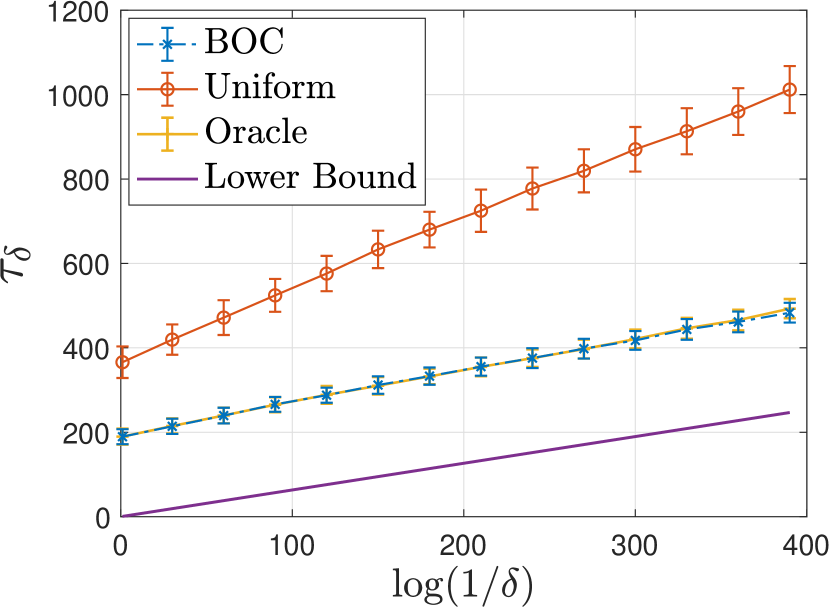
(a) The easy instance with $\beta(\delta,t)$.

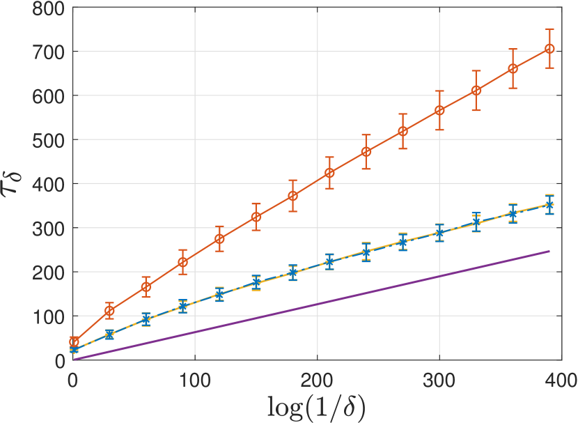
(b) The easy instance with $\tilde{\beta}(\delta,t)$.

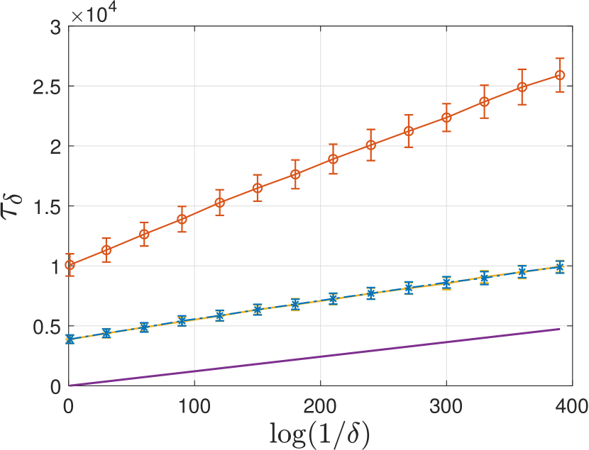
(c) The moderate instance with $\beta(\delta,t)$.

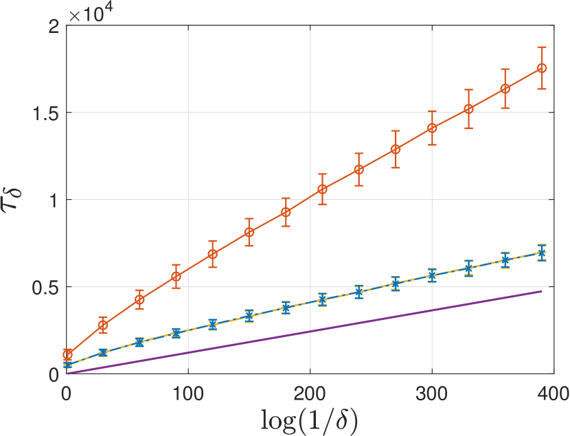
(d) The moderate instance with $\tilde{\beta}(\delta,t)$.

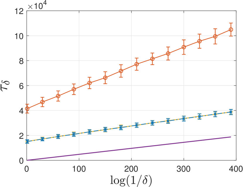
(e) The challenging instance with $\beta(\delta,t)$.

(f) The challenging instance with $\tilde{\beta}(\delta,t)$.

The empirical averaged sample complexities of the different methods with the two kinds of threshold functions for different confidence levels $\delta$ on the synthetic dataset.

The experimental results of the different methods with the two kinds of threshold functions for different confidence levels $\delta$ are presented in Figure 6.1. To better demonstrate the asymptotic behavior, we plot the empirical averaged sample complexities of the three methods as well as the instance-dependent lower bound of the expected sample complexity (see Theorem 4.1) with respect to $\log(1/\delta)$ in the each sub-figure. From Figure 6.1, we have the following observations:

• Although our algorithm BOC does not require the optimal oracle sampling rule $\lambda^{*}$, and instead approximates it on the fly, the curves of BOC and Oracle in the each sub-figure are almost completely overlapping, which suggests the proportion of arm pulls for BOC converges to the distribution $\lambda^{*}$ very quickly.

• The main observation is that as $\delta$ decreases (or equivalently, as $\log(1/\delta)$ increases), the slope of the curve corresponding to the BOC algorithm in the each sub-figure is almost equal to the slope of the lower bound, which is exactly equal to $D^{*}(c,\mathcal{U})$. However, the slope of the curve corresponding to Uniform is consistently larger than that of the lower bound, exemplifying its suboptimality. This suggests that the expected sample complexity of our algorithm BOC matches the instance-dependent lower bound asymptotically, corroborating our theoretical results (see the lower bound and upper bound in Theorems 4.1 and 5.10, respectively).

• There are unavoidable gaps between the lower bound and BOC (or, almost equivalently, Oracle), which is not an unexpected phenomenon. Although we have shown that the sampling rule resulting in $\lambda^{*}$ is asymptotically optimal, we have to utilize the stopping rule to evaluate the quality of the final recommendation (i.e., whether the recommended partition has an error probability of at most $\delta$). In addition, our bounds are only guaranteed to be tight asymptotically as $\delta\to 0$.

• Comparing the results for the same instance with the two different threshold functions, it can be seen that the heuristic one $\tilde{\beta}(\delta,t)$ leads to lower sample complexities, especially for large $\delta$ (i.e., small $\log(1/\delta)$). Even though there are no theoretical guarantees when $\tilde{\beta}(\delta,t)$ is used in our stopping rule, this threshold appears to work well empirically.

6.2 Real-world Datasets: The Iris and Yeast Datasets

To complement the experiments on synthetic data and to verify that BOC also excels in the non-asymptotic regime, we conduct experiments on the Iris and Yeast datasets (Dua and Graff 2017), both of which are ubiquitous in offline clustering and classification tasks. Here, we perform a novel task—online clustering with bandit feedback. In the Iris dataset, the number of clusters $K=3$, the number of arms $M=150$, and the dimension $d=4$, while in the Yeast dataset, $K=10$, $M=1484$, and $d=8$. Note that the total number of partitions grows asymptotically as $K^{M}/K!$ (i.e., approximately $10^{70}$ or $10^{1477}$ in the Iris and Yeast datasets, respectively); hence, it is impractical to exhaustively enumerate over all partitions in these datasets. We emphasize that BOC succeeds in circumventing the need to solve any NP-hard optimization problem as a subroutine in the online clustering task. To adapt these datasets to be amenable to online clustering tasks, we choose each cluster center to be the mean of the original data points of the arms in it, and then rescale the centers so that the hardness parameter $D^{*}(c,\mathcal{U})$ is equal to $2$ for both datasets. Since the performances of BOC and Oracle are similar (as observed in Section 6.1) and the heuristic threshold function $\tilde{\beta}(\delta,t)$ generally achieves lower sample complexities (compared to when $\beta(t,\delta)$ is used), we only present the results of the two methods (namely BOC and Uniform) with $\tilde{\beta}(\delta,t)$ on the two real datasets.

The averaged empirical sample complexities of BOC and Uniform with the heuristic threshold function $\tilde{\beta}(\delta,t)$ for different confidence levels $\delta$ on the real-world datasets.      Iris Dataset      Yeast Dataset      $\delta$      BOC      Uniform      BOC      Uniform      $10^{-1}$      883.3 $\pm$ 52.8      1174.8 $\pm$ 65.3      14430.5 $\pm$ 371.3      19536.0 $\pm$ 530.4      $10^{-2}$      922.2 $\pm$ 63.5      1208.1 $\pm$ 65.8      14531.2 $\pm$ 273.4      19697.4 $\pm$ 636.2      $10^{-3}$      963.1 $\pm$ 88.3      1245.2 $\pm$ 71.0      14589.5 $\pm$ 175.2      19997.4 $\pm$ 718.7      $10^{-4}$      989.5 $\pm$ 88.4      1282.1 $\pm$ 73.5      14631.5 $\pm$ 101.6      20220.3 $\pm$ 679.2      $10^{-5}$      1032.7 $\pm$ 80.6      1303.3 $\pm$ 74.0      14639.6 $\pm$ 150.0      20467.7 $\pm$ 591.0      $10^{-6}$      1054.6 $\pm$ 72.6      1338.3 $\pm$ 68.3      14686.3 $\pm$ 218.1      20564.5 $\pm$ 499.3      $10^{-7}$      1078.3 $\pm$ 63.6      1366.3 $\pm$ 70.6      14723.8 $\pm$ 270.3      20686.5 $\pm$ 338.6      $10^{-8}$      1093.7 $\pm$ 54.8      1391.7 $\pm$ 73.1      14797.3 $\pm$ 348.5      20733.1 $\pm$ 240.6      $10^{-9}$      1101.6 $\pm$ 50.9      1410.2 $\pm$ 74.6      14844.6 $\pm$ 385.7      20762.0 $\pm$ 132.4      $10^{-10}$      1117.4 $\pm$ 49.0      1450.0 $\pm$ 76.5      14977.1 $\pm$ 445.0      20766.8 $\pm$ 107.1

The sample complexities for different confidence levels $\delta$ are presented in Table 6.2. From the table, we see that BOC significantly outperforms the non-adaptive baseline method Uniform for all $\delta$ in terms of sample complexities. This demonstrates that BOC is able to effectively learn the clusters in an online manner given bandit feedback.

7 Conclusion

In this paper, we proposed a novel online clustering with bandit feedback framework in which there is a set of arms that can be clustered into non-overlapping groups, and at each time, one arm is pulled, and a sample from the distribution it is associated with is observed. We proposed and analyzed Bandit Online Clustering (or BOC) that, as discussed in Section 5.3, overcomes some critical computational limitations that a standard and natural GLR statistic suffers from due to the combinatorial search space of partitions. In addition to its computational efficiency, we proved that BOC is asymptotically optimal in the sense that it attains an instance-dependent information-theoretic lower bound as the confidence level $\delta$ tends to zero.

There are some limitations of the current model and theoretical contributions that serve as fertile avenues for future research. Firstly, in real-world applications such as recommendation systems and online market segmentation, it is often the case that the absolute correct clustering does not have to be found; an approximate clustering, with the advantage of further computational reductions, is usually sufficient. Developing computationally efficient and statistically optimal algorithms that allow for some distortion from the optimal clustering is thus of practical and theoretical importance. Secondly, our results are asymptotic in nature; they are only tight when the confidence level $\delta$ tends to zero. As we have seen in Section 6, this results in a gap between the upper bound and the actual performance of BOC when $\delta$ is not vanishingly small. It would thus be instructive to develop non-asymptotic or refined asymptotic bounds, perhaps by leveraging the “second-order” results in Malyutov and Tsitovich (2001) and Li and Tan (2020). Finally, it is worth developing bandit feedback models and algorithms for other generalizations of clustering, such as hierarchical clustering, fuzzy or soft clustering, or community detection on graphs (Abbe 2017).

8 Auxiliary Lemmas

Lemma 8.1 (The Maximum Theorem (Berge 1963, Sundaram 1996))

Let $f:S\times\Theta\to\mathbb{R}$ be a continuous function , and $\mathcal{D}:\Theta\rightrightarrows S$ be a compact-valued continuous correspondence. Let $f^{*}:\Theta\to\mathbb{R}$ and $D^{*}:\Theta\rightrightarrows S$ be defined by

$$f^{*}(\theta)=\max\{f(x,\theta):x\in\mathcal{D}(\theta)\}$$

and

$$\mathcal{D}^{*}(\theta)=\argmax\{f(x,\theta):x\in\mathcal{D}(\theta)\}=\{x\in\mathcal{D}(\theta):f(x,\theta)=f^{*}(\theta)\}.$$

Then $f^{*}$ is a continuous function on $\Theta$, and $\mathcal{D}^{*}$ is a compact-valued, upper hemicontinuous correspondence on $\Theta$.

Lemma 8.2 (Sundaram (1996, Theorem 9.12))

A single-valued correspondence that is hemicontinuous (whether upper or lower hemicontinuous) is continuous when viewed as a function. Conversely, every continuous function, when viewed as a single-valued correspondence, is both upper and lower hemicontinuous.

Lemma 8.3

Let $\lambda^{*}$ denote the oracle optimal sampling rule of the instance $(c,\mathcal{U})$. If there exists $\epsilon>0$ and $t_{0}(\epsilon)$ such that

$$\sup_{t\geq t_{0}(\epsilon)}\max_{m\in[M]}|\lambda^{*}_{m}(t)-\lambda^{*}_{m}|\leq\epsilon,$$

then there exists $t_{1}(\epsilon)\geq t_{0}(\epsilon)$ such that

$$\sup_{t\geq t_{1}(\epsilon)}\max_{m\in[M]}\left|\frac{N_{m}(t)}{t}-\lambda^{*}_{m}\right|\leq 3(M-1)\epsilon.$$

Furthermore, a valid choice of $t_{1}(\epsilon)$ is $\frac{t_{0}(\epsilon)}{\epsilon^{3}}$.

Proof 8.4

Proof of Lemma 8.3. Our sampling rule satisfies the assumptions of Garivier and Kaufmann (2016, Lemma 17), and the existence of $t_{1}(\epsilon)$ follows. The choice of $t_{1}(\epsilon)$ can be obtained by working through the proof of the same lemma.

Lemma 8.5

For any $x,y\in\mathbb{R}^{+}$,

$$\left(\left(-\sqrt{x}+\sqrt{y}\right)_{+}\right)^{2}=\max_{\alpha\geq 0}\left(-\alpha x+\frac{\alpha}{\alpha+1}y\right).$$

Proof 8.6

Proof of Lemma 8.5. Notice that

$$-\alpha x+\frac{\alpha}{\alpha+1}y=-(1+\alpha)x-\frac{1}{1+\alpha}y+(x+y).$$

If $y\geq x$, then

$$\max_{\alpha\geq 0}\left(-\alpha x+\frac{\alpha}{\alpha+1}y\right) =\left.\left(-(1+\alpha)x-\frac{1}{1+\alpha}y\right)\right|_{\alpha=\sqrt{\frac{y}{x}}-1}+(x+y)$$

$$=-2\sqrt{xy}+(x+y)$$

$$=\left(\left(-\sqrt{x}+\sqrt{y}\right)_{+}\right)^{2}.$$

If $y<x$, then

$$\max_{\alpha\geq 0}\left(-\alpha x+\frac{\alpha}{\alpha+1}y\right) =\left.\left(-(1+\alpha)x-\frac{1}{1+\alpha}y\right)\right|_{\alpha=0}+(x+y)$$

$$=0$$

$$=\left(\left(-\sqrt{x}+\sqrt{y}\right)_{+}\right)^{2}.$$

Lemma 8.7

For any $x,y\in\mathbb{R}^{d}$ and $\alpha\geq 0$,

$$-\alpha\|x\|^{2}+\frac{\alpha}{\alpha+1}\|y\|^{2}\leq\|x-y\|^{2}.$$

Proof 8.8

Proof of Lemma 8.7. Notice that the above inequality is equivalent to

$$\phantom{\;\iff\;}(1+\alpha)\|x\|^{2}-2x\cdot y+\frac{1}{\alpha+1}\|y\|^{2}\geq 0,$$

which is equivalent to

$$\left\|\sqrt{1+\alpha}\cdot x-\frac{1}{\sqrt{\alpha+1}}\cdot y\right\|^{2}\geq 0.$$

Thus, the result obviously holds.

Lemma 8.9

It holds that

$$\Pr\left(\exists\,t\in\mathbb{N}:\frac{1}{2}\sum_{m=1}^{M}N_{m}(t)\|\hat{\mu}_{m}(t)-\mu(c_{m})\|^{2}\geq\beta(\delta,t)\right)\leq\delta$$

where $\beta(\delta,t)$ is defined in Equation (8).

Proof 8.10

Proof of Lemma 8.9. In this proof, we use $[x]_{i}$ to denote the $i^{\mathrm{th}}$ component of the vector $x\in\mathbb{R}^{d}$.

Recall that at each time $t$, the agent selects an arm $A_{t}$ and observes $X_{t}=\mu(c_{A_{t}})+\eta_{t}$, where $\eta_{t}$ follows the standard $d$-dimensional Gaussian distribution $\mathcal{N}(\mathbf{0},\mathbf{I}_{d})$. Since each individual component of $\eta_{t}$ independently follows the standard univariate Gaussian distribution $\mathcal{N}(0,1)$, one arbitrary arm can be treated as $d$ independent sub-arms. Equivalently, the agent selects a group of $d$ sub-arms and observes

$$[X_{t}]_{i}=\left[\mu(c_{A_{t}})\right]_{i}+[\eta_{t}]_{i}$$

for all $i\in[d]$.

Note that there are $Md$ sub-arms in total. Then Lemma 8.9 follows from the concentration inequality for the empirical means of sub-arms (Kaufmann and Koolen 2021, Theorem 9).

Lemma 8.11 (Adapted from Garivier and Kaufmann (2016, Lemma 18))

For any two constants $a>0$ and $b\in\mathbb{R}$ such that $b+\log\left(\frac{1}{a}\right)>0$,

$$x=\frac{1}{a}\left(b+\log\left(\frac{e}{a}\right)+\log\left(b+\log\left(\frac{1}{a}\right)\right)\right)$$

satisfies $ax\geq\log(x)+b$.

9 Proofs of Section 4

9.1 Proof of Theorem 4.1

Proof 9.1

Proof of Theorem 4.1. For fixed $\delta\in(0,1)$ and instance $(c,\mathcal{U})$, consider any $\delta$-PAC online clustering algorithm.

We will see in Proposition 4.5 that $D^{*}(c,\mathcal{U})$ is finite so the situation that $\operatorname{\mathbb{E}}[\tau_{\delta}]$ is infinite is trivial. Henceforth, we assume that $\operatorname{\mathbb{E}}[\tau_{\delta}]$ is finite.

For any arm $m\in[M]$, let $N_{m}(t)$ denote the number of pulls of arm $m$ up to time $t$. Consider an arbitrary instance $(c^{\prime},\mathcal{U}^{\prime})$ in $\mathrm{Alt}(c)$. By applying the transportation inequality (Kaufmann et al. 2016, Lemma 1) and the KL-divergence for the multivariate normal distribution, we have

$$\frac{1}{2}\sum_{m=1}^{M}\operatorname{\mathbb{E}}[N_{m}(\tau_{\delta})]\|\mu(c_{m})-\mu^{\prime}(c^{\prime}_{m})\|^{2}\geq{d_{\mathrm{KL}}(\delta,1-\delta)}.$$

Since the above displayed inequality holds for all instances in $\mathrm{Alt}(c)$ and $[\operatorname{\mathbb{E}}[N_{1}(\tau_{\delta})],\operatorname{\mathbb{E}}[N_{2}(\tau_{\delta})],\ldots,\operatorname{\mathbb{E}}[N_{M}(\tau_{\delta})]]^{\top}/\operatorname{\mathbb{E}}[\tau_{\delta}]$ forms a probability distribution in $\mathcal{P}_{M}$, we obtain

$${d_{\mathrm{KL}}(\delta,1-\delta)} \leq\frac{1}{2}\inf_{(c^{\prime},\mathcal{U}^{\prime})\in\mathrm{Alt}(c)}\sum_{m=1}^{M}\operatorname{\mathbb{E}}[N_{m}(\tau_{\delta})]\|\mu(c_{m})-\mu^{\prime}(c^{\prime}_{m})\|^{2}$$

$$=\frac{1}{2}\operatorname{\mathbb{E}}[\tau_{\delta}]\inf_{(c^{\prime},\mathcal{U}^{\prime})\in\mathrm{Alt}(c)}\sum_{m=1}^{M}\frac{\operatorname{\mathbb{E}}[N_{m}(\tau_{\delta})]}{\operatorname{\mathbb{E}}[\tau_{\delta}]}\|\mu(c_{m})-\mu^{\prime}(c^{\prime}_{m})\|^{2}$$

$$\leq\frac{1}{2}\operatorname{\mathbb{E}}[\tau_{\delta}]\sup_{\lambda\in\mathcal{P}_{M}}\inf_{(c^{\prime},\mathcal{U}^{\prime})\in\mathrm{Alt}(c)}\sum_{m=1}^{M}\lambda_{m}\|\mu(c_{m})-\mu^{\prime}(c^{\prime}_{m})\|^{2}$$

$$=\operatorname{\mathbb{E}}[\tau_{\delta}]D^{*}(c,\mathcal{U})^{-1}.$$

Since $\lim_{\delta\rightarrow 0}{d_{\mathrm{KL}}(\delta,1-\delta)}/{\log(1/\delta)}=1$, letting $\delta\to 0$ yields

$$\liminf_{\delta\rightarrow 0}\frac{\operatorname{\mathbb{E}}[\tau_{\delta}]}{\log(1/\delta)}\geq D^{*}(c,\mathcal{U})$$

as desired.

9.2 Proof of Lemma 4.2

Proof 9.2

Proof of Lemma 4.2. For any fixed $\lambda\in\mathcal{P}_{M}$ and $(c^{\prime},\mathcal{U}^{\prime})$, let

$$\mathrm{Dist}(c^{\prime},\mathcal{U}^{\prime}):=\sum_{m=1}^{M}\lambda_{m}\|\mu(c_{m})-\mu^{\prime}(c^{\prime}_{m})\|^{2}.$$

To prove Lemma 4.2, we only need to show for any instance $(c^{\dagger},\mathcal{U}^{\dagger})\in\mathrm{Alt}(c)$ such that $d_{\mathrm{H}}(c^{\dagger},c)>1$, there exists another instance $(c^{*},\mathcal{U}^{*})\in\mathrm{Alt}(c)$ such that $d_{\mathrm{H}}(c^{*},c)=1$ and $\mathrm{Dist}(c^{*},\mathcal{U}^{*})\leq\mathrm{Dist}(c^{\dagger},\mathcal{U}^{\dagger})$. The proof consists of four steps and Figure 9.2 serves as an illustration to help understand the various constructions.

\begin{overpic}[width=433.62pt]{figs/lemma1.pdf} \put(7.8,65.28){{Step 1}} \put(7.8,47.0){{Step 2}} \put(7.8,19.68){{Step 3}} \put(24.0,69.0){{$c^{\phantom{(0)}}:$}} \put(24.0,60.6){{$c^{(0)}:$}} \put(24.0,50.7){{$c^{\phantom{(1)}}:$}} \put(24.0,42.3){{$c^{(1)}:$}} \put(24.0,32.2){{$c^{\phantom{(2)}}:$}} \put(24.0,23.8){{$c^{(2)}:$}} \put(24.0,15.9){{$c^{\phantom{(3)}}:$}} \put(24.0,7.4){{$c^{(3)}:$}} \end{overpic}

An illustration of the proof of Lemma 4.2. Figure 9.2 illustrates the construction of the sequence of instances when the number of clusters $K=3$ and the number of arms (or items) $M=9$. Each pair of items connected by a double arrow represents the cluster indices of one arm in the true partition $c$ and one of the newly constructed partitions $c^{(\bar{k})}$ for $\bar{k}=0,1,2,3$. After the application of the permutation $\sigma$ as defined in (14) in Step 1, each of the arms can have any cluster index. However, due to the desirable property of the permutation as stated in (20), in Step 2, we are able to construct a new partition $c^{(1)}$ such that for any arm, its cluster index in $c^{(1)}$ is not larger than that of $c$. Next, we modify the new partition from right to left in Step 3 (see Equations (22) and (23)) and we finally return to a partition that is identical to $c$.

Step 1 (Permute the partition of the given instance). To construct a new instance, we construct a permutation $\sigma$ on $[K]$ such that

$$\left\{\begin{array}[]{l}\sigma^{-1}(1)=\argmin\limits_{k\in[K]}\|\mu^{\dagger}(k)-\mu(1)||^{2}\\ \sigma^{-1}(2)=\argmin\limits_{k\in[K]\setminus\{\sigma^{-1}(1)\}}\|\mu^{\dagger}(k)-\mu(2)||^{2}\\ \sigma^{-1}(3)=\argmin\limits_{k\in[K]\setminus\{\sigma^{-1}(1),\sigma^{-1}(2)\}}\|\mu^{\dagger}(k)-\mu(3)||^{2}\\ \cdots\\ \sigma^{-1}(K-1)=\argmin\limits_{k\in[K]\setminus\{\sigma^{-1}(1),\sigma^{-1}(2),\ldots\sigma^{-1}(K-2)\}}\|\mu^{\dagger}(k)-\mu(K-1)||^{2}.\end{array}\right.$$ (14)

Let $(c^{(0)},\mathcal{U}^{(0)})=\sigma(c^{\dagger},\mathcal{U}^{\dagger})$ and hence we have

$$\left\{\begin{array}[]{l}1=\argmin\limits_{1\leq k\leq K}\|\mu^{(0)}(k)-\mu(1)||^{2}\\ 2=\argmin\limits_{2\leq k\leq K}\|\mu^{(0)}(k)-\mu(2)||^{2}\\ 3=\argmin\limits_{3\leq k\leq K}\|\mu^{(0)}(k)-\mu(3)||^{2}\\ \cdots\\ K-1=\argmin\limits_{K-1\leq k\leq K}\|\mu^{(0)}(k)-\mu(K-1)||^{2}.\end{array}\right.$$ (20)

Obviously, $d_{\mathrm{H}}(c,c^{(0)})\geq 1$, otherwise $(c^{\dagger},\mathcal{U}^{\dagger})\not\in\mathrm{Alt}(c)$.

Step 2 (Update the clustering). Now we construct another instance $(c^{(1)},\mathcal{U}^{(0)})$, in which $c^{(1)}_{m}=\min(c_{m},c^{(0)}_{m})$ for all $m\in[M]$. It holds that

$$\mathrm{Dist}(c^{(0)},\mathcal{U}^{(0)}) =\sum_{m=1}^{M}\lambda_{m}\|\mu(c_{m})-\mu^{(0)}(c^{(0)}_{m})\|^{2}$$

$$=\sum_{m=1}^{M}\lambda_{m}\|\mu(c_{m})-\mu^{(0)}(c^{(0)}_{m})\|^{2}\mathbbm{1}\{c_{m}\leq c^{(0)}_{m}\}+\sum_{m=1}^{M}\lambda_{m}\|\mu(c_{m})-\mu^{(0)}(c^{(0)}_{m})\|^{2}\mathbbm{1}\{c_{m}>c^{(0)}_{m}\}$$

$$\geq\sum_{m=1}^{M}\lambda_{m}\|\mu(c_{m})-\mu^{(0)}(c_{m})\|^{2}\mathbbm{1}\{c_{m}\leq c^{(0)}_{m}\}+\sum_{m=1}^{M}\lambda_{m}\|\mu(c_{m})-\mu^{(0)}(c^{(0)}_{m})\|^{2}\mathbbm{1}\{c_{m}>c^{(0)}_{m}\}$$

$$=\sum_{m=1}^{M}\lambda_{m}\|\mu(c_{m})-\mu^{(0)}(c^{(1)}_{m})\|^{2}$$

$$=\mathrm{Dist}(c^{(1)},\mathcal{U}^{(0)})$$

where the inequality is due to our construction of $(c^{(0)},\mathcal{U}^{(0)})$ in Equation (20).

Step 3 (Construct a sequence of instances). For any $(c^{\prime},\mathcal{U}^{\prime})$ and $k,k^{\prime}\in[K]$, let

$$w_{k,k^{\prime}}(c^{\prime}):=\sum_{m=1}^{M}\lambda_{m}\mathbbm{1}\{c_{m}=k,c^{\prime}_{m}=k^{\prime}\}.$$

Then

$$\mathrm{Dist}(c^{\prime},\mathcal{U}^{\prime})=\sum_{k=1}^{K}\sum_{k^{\prime}=1}^{K}w_{k,k^{\prime}}(c^{\prime})\|\mu(k)-\mu^{\prime}(k^{\prime})\|^{2}.$$

Moreover, the minimization problem $\min_{\mathcal{U}^{\prime}}\mathrm{Dist}(c^{\prime},\mathcal{U}^{\prime})$ has a unique solution $\mathcal{U}^{\prime\star}$ which is defined by its components as

$$\mu^{\prime\star}(k^{\prime})=\frac{\sum_{k=1}^{K}w_{k,k^{\prime}}(c^{\prime})\mu(k)}{\sum_{k=1}^{K}w_{k,k^{\prime}}(c^{\prime})}$$ (21)

for all $k^{\prime}\in[K]$.

Consider an instance $(c^{(1)},\mathcal{U}^{(1)})$, in which $\mathcal{U}^{(1)}=\argmin_{\mathcal{U}^{\prime}}\mathrm{Dist}(c^{(1)},\mathcal{U}^{\prime})$. Clearly, it holds that $\mathrm{Dist}(c^{(1)},\mathcal{U}^{(0)})\geq\mathrm{Dist}(c^{(1)},\mathcal{U}^{(1)})$. From the construction of $c^{(1)}$, we also know that $w_{k,K}(c^{(1)})=0$ for any $k\neq K$. Therefore, by (21), $\mu^{(1)}(K)=\mu(K)$.

Then consider another instance $(c^{(2)},\mathcal{U}^{(1)})$, where

$$c^{(2)}_{m}=\begin{cases}K&\text{if }c_{m}=K\\ c^{(1)}_{m}&\text{otherwise.}\end{cases}$$ (22)

Since $\mu^{(1)}(K)=\mu(K)$, $\mathrm{Dist}(c^{(1)},\mathcal{U}^{(1)})\geq\mathrm{Dist}(c^{(2)},\mathcal{U}^{(1)})$. Next, we construct $(c^{(2)},\mathcal{U}^{(2)})$, in which $\mathcal{U}^{(2)}=\argmin_{\mathcal{U}^{\prime}}\mathrm{Dist}(c^{(2)},\mathcal{U}^{\prime})$. From the construction of $c^{(2)}$, we also know that $w_{k,K-1}(c^{(2)})=0$ for any $k\neq K-1$. Therefore, $\mu^{(2)}(K-1)=\mu(K-1)$ and $\mathrm{Dist}(c^{(2)},\mathcal{U}^{(2)})\geq\mathrm{Dist}(c^{(3)},\mathcal{U}^{(2)})$ where

$$c^{(3)}_{m}=\begin{cases}K-1&\text{if }c_{m}=K-1\\ c^{(2)}_{m}&\text{otherwise.}\end{cases}$$ (23)

Following the same method, we can then construct a sequence of instances $\{(c^{(3)},\mathcal{U}^{(3)}),(c^{(4)},\mathcal{U}^{(3)}),\ldots,(c^{(K)},\mathcal{U}^{(K)})\}$. Note that eventually $(c^{(K)},\mathcal{U}^{(K)})=(c,\mathcal{U})$ since the cluster indices of $c^{(K)}$ and $c$ are the same and $\mathcal{U}^{(K)}=\argmin_{\mathcal{U}^{\prime}}\mathrm{Dist}(c^{(K)},\mathcal{U}^{\prime})$.

Step 4 (Find the desired instance within the constructed sequence). Consider the whole sequence $\{(c^{(0)},\mathcal{U}^{(0)}),(c^{(1)},\mathcal{U}^{(0)}),(c^{(1)},\mathcal{U}^{(1)}),(c^{(2)},\mathcal{U}^{(1)}),\ldots,(c^{(K)},\mathcal{U}^{(K)})\}$. Both the distance function $\mathrm{Dist}(\cdot,\cdot)$ and the Hamming distance $d_{\mathrm{H}}(c,\cdot)$ are non-increasing. Furthermore, $d_{\mathrm{H}}(c,c^{(K)})=0$.

If $d_{\mathrm{H}}(c,c^{(0)})=1$, we can simply choose $(c^{*},\mathcal{U}^{*})=(c^{(0)},\mathcal{U}^{(0)})$.

If $d_{\mathrm{H}}(c,c^{(0)})>1$, from the sequence of instances, we can select the first instance whose partition is exactly the same as $c$, denoted as $(c^{(\bar{k})},\mathcal{U}^{(\bar{k}-1)})$ ($1\leq\bar{k}\leq K$), i.e., $c^{(\bar{k})}=c$. We also know $(c^{(\bar{k}-1)},\mathcal{U}^{(\bar{k}-1)})$ satisfies that $d_{\mathrm{H}}(c,c^{(\bar{k}-1)})\geq 1$.

Our construction of the sequence of instances is “consecutive” in the sense that we can modify the cluster indices of $c^{(\bar{k}-1)}$ one by one until we get exactly the partition $c^{(\bar{k})}$. Therefore, we can construct another sequence of instances $\{(c^{(\bar{k}-1)},\mathcal{U}^{(\bar{k}-1)}),(c^{(\bar{k}^{\prime}-1)},\mathcal{U}^{(\bar{k}-1)}),(c^{(\bar{k}^{\prime\prime}-1)},\mathcal{U}^{(\bar{k}-1)}),\ldots,(c^{(\bar{k})},\mathcal{U}^{(\bar{k}-1)})\}$, where the Hamming distance $d_{\mathrm{H}}(c,\cdot)$ is strictly decreasing by $1$ in each step in this sequence. Besides, the distance function $\mathrm{Dist}(\cdot,\cdot)$ is also non-increasing. As a result, we can always find an instance $(c^{*},\mathcal{U}^{*})$ in this sequence such that $d_{\mathrm{H}}(c^{*},c)=1$.

9.3 Proof of Proposition 4.3

Proof 9.3

Proof of Proposition 4.3. Due to Lemma 4.2, we only need to consider the set of alternative instances $\{(c^{\prime},\mathcal{U}^{\prime})\in\mathrm{Alt}(c):d_{\mathrm{H}}(c^{\prime},c)=1\}$.

If $\lambda\in\mathcal{P}_{M}^{+}$, suppose that $c$ and $c^{\prime}$ only differ in the label of arm $m$, which is changed from $c_{m}$ to $k^{\prime}$. Since $c^{\prime}$ is a valid partition, we have $n(c_{m})>1$. To minimize the objective function, for any $k\in[K]\setminus\{k^{\prime}\}$, $\mu^{\prime}(k)$ can be exactly set to be $\mu(k)$. Therefore, the objective function can be simplified to

$$\lambda_{m}\|\mu(c_{m})-\mu^{\prime}(k^{\prime})\|^{2}+w(k^{\prime})\|\mu(k^{\prime})-\mu^{\prime}(k^{\prime})\|^{2},$$

which shows the mean vector of cluster $k^{\prime}$ should be chosen as $\mu^{\prime}(k^{\prime})=\frac{\lambda_{m}\mu(c_{m})+w(k^{\prime})\mu(k^{\prime})}{\lambda_{m}+w(k^{\prime})}$, a weighted sum of $\mu(c_{m})$ and $\mu(k^{\prime})$.

Altogether, the optimal value can be derived as follows:

$$\phantom{\;=\;}\inf_{(c^{\prime},\mathcal{U}^{\prime})\in\mathrm{Alt}(c)}\sum_{m=1}^{M}\lambda_{m}\|\mu(c_{m})-\mu^{\prime}(c^{\prime}_{m})\|^{2}$$

$$=\inf_{\begin{subarray}{c}(c^{\prime},\mathcal{U}^{\prime})\in\mathrm{Alt}(c):\\ d_{\mathrm{H}}(c^{\prime},c)=1\end{subarray}}\sum_{m=1}^{M}\lambda_{m}\|\mu(c_{m})-\mu^{\prime}(c^{\prime}_{m})\|^{2}$$

$$=\inf_{\begin{subarray}{c}m\in[M],k^{\prime}\in[K]:\\ n(c_{m})>1,k^{\prime}\neq c_{m}\end{subarray}}\frac{\lambda_{m}w(k^{\prime})}{\lambda_{m}+w(k^{\prime})}\|\mu(c_{m})-\mu(k^{\prime})\|^{2}$$ (24)

$$=\min_{\begin{subarray}{c}m\in[M],k^{\prime}\in[K]:\\ n(c_{m})>1,k^{\prime}\neq c_{m}\end{subarray}}\frac{\lambda_{m}w(k^{\prime})}{\lambda_{m}+w(k^{\prime})}\|\mu(c_{m})-\mu(k^{\prime})\|^{2}$$ (25)

$$=\min_{\begin{subarray}{c}k,k^{\prime}\in[K]:\\ n(k)>1,k^{\prime}\neq k\end{subarray}}\frac{\bar{w}(k)w(k^{\prime})}{\bar{w}(k)+w(k^{\prime})}\|\mu(k)-\mu(k^{\prime})\|^{2}$$ (26)

where Equation (24) follows from our choice of the mean vectors above and Equation (26) follows from the fact that for any $y,z>0$, $f(x)=\frac{xy}{x+z}$ is increasing on $(0,\infty)$. As a consequence, the infimum in Problem ($\bigtriangleup$) can be replaced with a minimum since the infimum can be attained by some ${(c^{\prime},\mathcal{U}^{\prime})\in\mathrm{Alt}(c)}$.

If $\lambda\in\mathcal{P}_{M}\setminus\mathcal{P}_{M}^{+}$, suppose that $\lambda_{m}=0$ for some $m\in[M]$. Notice that the objective function is always non-negative.

We consider two situations. First, if $n(c_{m})>1$, we will construct an instance $(c^{\prime},\mathcal{U}^{\prime})\in\mathrm{Alt}(c)$ such that the objective function is zero. In particular, we can change the label of the arm $m$ from $c_{m}$ to any $k\neq c_{m}$, and keep all the mean vectors the same. Then the objective function for the new instance is exactly zero, which shows

$$\inf_{(c^{\prime},\mathcal{U}^{\prime})\in\mathrm{Alt}(c)}\sum_{m=1}^{M}\lambda_{m}\|\mu(c_{m})-\mu^{\prime}(c^{\prime}_{m})\|^{2}=0.$$

Second, if $n(c_{m})=1$, we will construct an instance $(c^{\prime},\mathcal{U}^{\prime})\in\mathrm{Alt}(c)$ such that the objective function is arbitrarily close to zero. In particular, we can change the label of any other arm $m^{\prime}$ (subject to $n(c_{m^{\prime}})>1$) from $c_{m^{\prime}}$ to $c_{m}$. Thus the objective function can be simplified to

$$\lambda_{m^{\prime}}\|\mu(c_{m^{\prime}})-\mu^{\prime}(c_{m})\|^{2}.$$

For the mean vector of $c_{m}$, note that we cannot set $\mu^{\prime}(c_{m})$ to be exactly $\mu(c_{m^{\prime}})$ otherwise $(c^{\prime},\mathcal{U}^{\prime})\notin\mathrm{Alt}(c)$. However, we can let $\mu^{\prime}(c_{m})$ be arbitrarily close to $\mu(c_{m^{\prime}})$, which yields

$$\inf_{(c^{\prime},\mathcal{U}^{\prime})\in\mathrm{Alt}(c)}\sum_{m=1}^{M}\lambda_{m}\|\mu(c_{m})-\mu^{\prime}(c^{\prime}_{m})\|^{2}=0.$$

This completes the proof of Proposition 4.3.

Remark 9.4

In fact, from the above proof, we know more about the optimal solution if $\lambda\in\mathcal{P}_{M}^{+}$. Let

$$(k^{*},k^{\prime*}):=\argmin_{\begin{subarray}{c}k,k^{\prime}\in[K]:\\ n(k)>1,k^{\prime}\neq k\end{subarray}}\frac{\bar{w}(k)w(k^{\prime})}{\bar{w}(k)+w(k^{\prime})}\|\mu(k)-\mu(k^{\prime})\|^{2}.$$

Then there exists $(c^{*},\mathcal{U}^{*})$, where

$$c^{*}_{m}=\begin{cases}k^{\prime*}&\text{if }m=\argmin_{m\in[M]:c_{m}=k^{*}}\lambda_{m}\\ c_{m}&\text{otherwise}\end{cases}$$

and

$$\mu^{*}(k)=\begin{cases}\frac{\bar{w}(k^{*})\mu(k^{*})+w(k^{\prime*})\mu(k^{\prime*})}{\bar{w}(k^{*})+w(k^{\prime*})}&\text{if }m=k^{\prime*}\\ \mu(k)&\text{otherwise}\end{cases}$$

such that

$$(c^{*},\mathcal{U}^{*})\in\argmin_{(c^{\prime},\mathcal{U}^{\prime})\in\mathrm{Alt}(c)}\sum_{m=1}^{M}\lambda_{m}\|\mu(c_{m})-\mu^{\prime}(c^{\prime}_{m})\|^{2}.$$

9.4 Proof of Proposition 4.4

Proof 9.5

Proof of Proposition 4.4. First, we define $f_{1}:\mathbb{R}^{+}\times\mathbb{R}^{+}\to\mathbb{R}^{+}$ as

$$f_{1}(x,y):=\begin{cases}\frac{xy}{x+y}&\text{ if }x+y\neq 0\\ 0&\text{ otherwise }\end{cases}$$

which is continuous on $\mathbb{R}^{+}\times\mathbb{R}^{+}$.

Next, we will prove that for all $(\lambda,\mathcal{U})\in\mathcal{P}_{M}\times\mathscr{U}$, $g(\lambda,\mathcal{U})$ as defined in Proposition 4.4 can be written as

$$g(\lambda,\mathcal{U})=\min_{\begin{subarray}{c}m\in[M],k\in[K]:\\ n(c_{m})>1,k\neq c_{m}\end{subarray}}f_{1}\left(\lambda_{m},\sum_{\bar{m}=1}^{M}\lambda_{\bar{m}}\mathbbm{1}\{c_{\bar{m}}=k\}\right)\|\mu(c_{m})-\mu(k)\|^{2}.$$ (27)

For any $\lambda\in\mathcal{P}_{M}^{+}$, Equation (27) follows directly from Equation (25) in the proof of Proposition 4.3.

For any $\lambda\in\mathcal{P}_{M}\setminus\mathcal{P}_{M}^{+}$, it suffices to find $m\in[M],k\in[K]$ subject to $n(c_{m})>1$ and $k\neq c_{m}$ such that $f_{1}\left(\lambda_{m},\sum_{\bar{m}=1}^{M}\lambda_{\bar{m}}\mathbbm{1}\{c_{\bar{m}}=k\}\right)=0$. Suppose that $\lambda_{\hat{m}}=0$ for some ${\hat{m}}\in[M]$ and we will consider two situations. If $n(c_{\hat{m}})>1$, we can simply choose $m=\hat{m}$ and any $k\neq c_{\hat{m}}$. If $n(c_{\hat{m}})=1$, we can choose any $m$ subject to $n(c_{m})>1$, and $k=c_{\hat{m}}$. Altogether, Equation (27) holds for all $(\lambda,\mathcal{U})\in\mathcal{P}_{M}\times\mathscr{U}$.

Finally, for any $m\in[M],k\in[K]$ such that $n(c_{m})>1$ and $k\neq c_{m}$, we consider the function

$$f_{2}(m,k;\lambda,\mathcal{U}):=f_{1}\left(\lambda_{m},\sum_{\bar{m}=1}^{M}\lambda_{\bar{m}}\mathbbm{1}\{c_{\bar{m}}=k\}\right)\|\mu(c_{m})-\mu(k)\|^{2}$$

so that

$$g(\lambda,\mathcal{U})=\min_{\begin{subarray}{c}m\in[M],k\in[K]:\\ n(c_{m})>1,k\neq c_{m}\end{subarray}}f_{2}(m,k;\lambda,\mathcal{U}).$$

Since $(\lambda,\mathcal{U})\mapsto f_{2}(m,k;\lambda,\mathcal{U})$ is continuous on $\mathcal{P}_{M}\times\mathscr{U}$ for fixed $m$ and $k$ and the finite minimum operation preserves continuity, $(\lambda,\mathcal{U})\mapsto g(\lambda,\mathcal{U})$ is also continuous on $\mathcal{P}_{M}\times\mathscr{U}$.

9.5 Proof of Proposition 4.5

Proof 9.6

Proof of Proposition 4.5. For any $(c,\mathcal{U})$, $D^{*}(c,\mathcal{U})$ can be written as:

$$D^{*}(c,\mathcal{U}) =\left\{\frac{1}{2}\sup_{\lambda\in\mathcal{P}_{M}}\inf_{(c^{\prime},\mathcal{U}^{\prime})\in\mathrm{Alt}(c)}\sum_{m=1}^{M}\lambda_{m}\|\mu(c_{m})-\mu^{\prime}(c^{\prime}_{m})\|^{2}\right\}^{-1}$$

$$=\left\{\frac{1}{2}\max_{\lambda\in\mathcal{P}_{M}}\inf_{(c^{\prime},\mathcal{U}^{\prime})\in\mathrm{Alt}(c)}\sum_{m=1}^{M}\lambda_{m}\|\mu(c_{m})-\mu^{\prime}(c^{\prime}_{m})\|^{2}\right\}^{-1}$$ (28)

$$=\left\{\frac{1}{2}\max_{\lambda\in\mathcal{P}_{M}^{+}}\min_{\begin{subarray}{c}k,k^{\prime}\in[K]:\\ n(k)>1,k^{\prime}\neq k\end{subarray}}\frac{\bar{w}(k)w(k^{\prime})}{\bar{w}(k)+w(k^{\prime})}\|\mu(k)-\mu(k^{\prime})\|^{2}\right\}^{-1}$$ (29)

$$=2\min_{\lambda\in\mathcal{P}_{M}^{+}}\max_{\begin{subarray}{c}k,k^{\prime}\in[K]:\\ n(k)>1,k^{\prime}\neq k\end{subarray}}\left(\frac{1}{\bar{w}(k)}+\frac{1}{w(k^{\prime})}\right)\|\mu(k)-\mu(k^{\prime})\|^{-2}.$$

where Equation (28) follows from the continuity of $g(\lambda,\mathcal{U})$ as shown in Proposition 4.4 and the compactness of $\mathcal{P}_{M}$, and Equation (29) follows from Proposition 4.3 and the non-negativity of $D^{*}(c,\mathcal{U})$.

Notice that both $\{w(k)\}_{k=1}^{K}$ and $\{\bar{w}(k)\}_{k=1}^{K}$ depend on $\lambda$. For any $k$ and fixed $w(k)$, $\bar{w}(k)=\min_{m\in[M]:c_{m}=k}\lambda_{m}$ is maximized if and only if for all $m\in[M]$ such that $c_{m}=k$, $\lambda_{m}$ are equal. Therefore, we can solve the outer minimization on a “smaller” probability simplex $\mathcal{P}_{K}^{+}$. This yields

$$D^{*}(c,\mathcal{U}) =2\min_{w\in\mathcal{P}_{K}^{+}}\max_{\begin{subarray}{c}k,k^{\prime}\in[K]:\\ n(k)>1,k^{\prime}\neq k\end{subarray}}\left(\frac{n(k)}{w(k)}+\frac{1}{w(k^{\prime})}\right)\|\mu(k)-\mu(k^{\prime})\|^{-2}.$$

9.6 Proof of Proposition 4.6

Proof 9.7

Proof of Proposition 4.6. According to the proof of Proposition 4.5, there exists a bijective map (which is specified in the proof of Proposition 4.5 as well as the statement of Proposition 4.6) between the solution(s) to

$$\argmax\limits_{\lambda\in\mathcal{P}_{M}}\inf\limits_{(c^{\prime},\mathcal{U}^{\prime})\in\mathrm{Alt}(c)}\sum\limits_{m=1}\limits^{M}\lambda_{m}\|\mu(c_{m})-\mu^{\prime}(c^{\prime}_{m})\|^{2}$$

and the solution(s) to

$$\argmin_{w\in\mathcal{P}_{K}^{+}}\max_{\begin{subarray}{c}k,k^{\prime}\in[K]:\\ n(k)>1,k^{\prime}\neq k\end{subarray}}\left(\frac{n(k)}{w(k)}+\frac{1}{w(k^{\prime})}\right)\|\mu(k)-\mu(k^{\prime})\|^{-2}.$$ (30)

Therefore, it suffices to show the solution to (30) is unique. We will show this by contradiction as follows.

Suppose that $w^{*}$ and $w^{**}$ are different solutions to (30) and $w^{*}({\hat{k}})\neq w^{**}({\hat{k}})$ for some $\hat{k}\in[K]$.

For any $k,k^{\prime}\in[K]$ such that $n(k)>1$ and $k^{\prime}\neq k$, consider the function

$$f_{1}(k,k^{\prime};w,\mathcal{U}):=2\left(\frac{n(k)}{w(k)}+\frac{1}{w(k^{\prime})}\right)\|\mu(k)-\mu(k^{\prime})\|^{-2}.$$

Since $\|\mu(k)-\mu(k^{\prime})\|^{-2}>0$ by the definition of $\mathscr{U}$, $f_{1}(k,k^{\prime};w,\mathcal{U})$ is convex in $w$. In particular, $f_{1}(k,k^{\prime};w,\mathcal{U})$ is strictly convex in the pair $(w(k),w(k^{\prime}))$. Besides, since the pointwise maximum operation preserves convexity,

$$f_{2}(w,\mathcal{U}):=\max_{\begin{subarray}{c}k,k^{\prime}\in[K]:\\ n(k)>1,k^{\prime}\neq k\end{subarray}}f_{1}(k,k^{\prime};w,\mathcal{U})$$

is also convex in $w$. Therefore, $w^{***}:=\frac{1}{2}(w^{*}+w^{**})$ is also a solution to (30) and

$$D^{*}(c,\mathcal{U})=f_{2}(w^{*},\mathcal{U})=f_{2}(w^{**},\mathcal{U})=f_{2}(w^{***},\mathcal{U}).$$

We claim that for any $k,k^{\prime}\in[K]$ such that $n(k)>1$ and $k^{\prime}\neq k$, if ${\hat{k}}\in\{k,k^{\prime}\}$, then

$$f_{1}(k,k^{\prime};w^{***},\mathcal{U})<D^{*}(c,\mathcal{U}).$$

Otherwise, using the fact $w^{*}({\hat{k}})\neq w^{**}({\hat{k}})$ and the strict convexity of $f_{1}(k,k^{\prime};w^{***},\mathcal{U})$ in the pair $(w^{***}(k),w^{***}(k^{\prime}))$,

$$D^{*}(c,\mathcal{U}) =f_{1}(k,k^{\prime};w^{***},\mathcal{U})$$

$$<\frac{1}{2}\left(f_{1}(k,k^{\prime};w^{*},\mathcal{U})+f_{1}(k,k^{\prime};w^{**},\mathcal{U})\right)$$

$$\leq\frac{1}{2}\left(f_{2}(w^{*},\mathcal{U})+f_{2}(w^{**},\mathcal{U})\right)$$

$$=D^{*}(c,\mathcal{U})$$

which leads to a contradiction. Therefore, our claim holds.

In view of this claim, we can identify a $w^{\dagger}\in\mathcal{P}_{K}^{+}$ such that $f_{2}(w^{\dagger},\mathcal{U})<D^{*}(c,\mathcal{U})$, which results in a contradiction to the optimality of $D^{*}(c,\mathcal{U})$. In particular, such a $w^{\dagger}$ can be defined through its components as

$$w^{\dagger}(k)=\begin{cases}w^{***}(k)-(K-1)\epsilon&\text{if }k=\hat{k}\\ w^{***}(k)+\epsilon&\text{otherwise}\end{cases}$$

with a sufficiently small $\epsilon>0$ such that

$$f_{1}(k,k^{\prime};w^{\dagger},\mathcal{U})<D^{*}(c,\mathcal{U})$$

for all $k,k^{\prime}\in[K]$ such that $n(k)>1$, $k^{\prime}\neq k$ and ${\hat{k}}\in\{k,k^{\prime}\}$. The existence of such a sufficiently small $\epsilon>0$ is guaranteed by the continuity of $f_{1}(k,k^{\prime};w^{***},\mathcal{U})$ in the pair $(w^{***}(k),w^{***}(k^{\prime}))$.

In addition, for any $k,k^{\prime}\in[K]$ such that $n(k)>1$, $k^{\prime}\neq k$ and ${\hat{k}}\not\in\{k,k^{\prime}\}$,

$$f_{1}(k,k^{\prime};w^{\dagger},\mathcal{U}) =2\left(\frac{n(k)}{w^{\dagger}(k)}+\frac{1}{w^{\dagger}(k^{\prime})}\right)\|\mu(k)-\mu(k^{\prime})\|^{-2}$$

$$<2\left(\frac{n(k)}{w^{***}(k)}+\frac{1}{w^{***}(k^{\prime})}\right)\|\mu(k)-\mu(k^{\prime})\|^{-2}$$

$$=f_{1}(k,k^{\prime};w^{***},\mathcal{U})$$

$$\leq D^{*}(c,\mathcal{U}).$$

In view of the fact that under both cases ($\hat{k}\in\{k,k^{\prime}\}$ and $\hat{k}\notin\{k,k^{\prime}\}$), we have $f_{1}(k,k^{\prime};w^{\dagger},U)<D^{*}(c,\mathcal{U})$, we conclude that

$$f_{2}(w^{\dagger},\mathcal{U})=\max_{\begin{subarray}{c}k,k^{\prime}\in[K]:\\ n(k)>1,k^{\prime}\neq k\end{subarray}}f_{1}(k,k^{\prime};w^{\dagger},\mathcal{U})<D^{*}(c,\mathcal{U})$$

which contradicts the fact that $D^{*}(c,\mathcal{U})$ is the optimal value.

Altogether, the solution to (30) is unique and hence the solution to

$$\argmax\limits_{\lambda\in\mathcal{P}_{M}}\inf\limits_{(c^{\prime},\mathcal{U}^{\prime})\in\mathrm{Alt}(c)}\sum\limits_{m=1}\limits^{M}\lambda_{m}\|\mu(c_{m})-\mu^{\prime}(c^{\prime}_{m})\|^{2}$$

is also unique.

9.7 Proof of Proposition 4.7

Proof 9.8

Proof of Proposition 4.7 Recalling Proposition 4.4,

$$g(\lambda,\mathcal{U})=\inf_{(c^{\prime},\mathcal{U}^{\prime})\in\mathrm{Alt}(c)}\sum_{m=1}^{M}\lambda_{m}\|\mu(c_{m})-\mu^{\prime}(c^{\prime}_{m})\|^{2}$$

is continuous on $\mathcal{P}_{M}\times\mathscr{U}$.

Since $\mathcal{P}_{M}$ does not depend on $\mathcal{U}$ and is compact, by Lemma 8.1,

$$\Lambda(\mathcal{U})=\argmax_{\lambda\in\mathcal{P}_{M}}g(\lambda,\mathcal{U})$$

is an upper hemicontinuous correspondence on $\mathscr{U}$.

According to Proposition 4.6, $\Lambda(\mathcal{U})$ is single-valued. Consequently, by Lemma 8.2, $\Lambda$ is continuous on $\mathscr{U}$.

10 Proofs of Section 5

10.1 Proof of Proposition 5.1

Proof 10.1

Proof of Proposition 5.1. The proof consists of three steps, using the triangle inequality frequently.

First, we show that the $K$ arms chosen in Maximin Initialization are selected from $K$ disjoint clusters.

Let $m_{1},m_{2},\ldots,m_{K}$ denote the arms chosen in Maximin Initialization in order. Assuming that we have already taken the empirical estimates of $\bar{k}$ arms as the cluster centers, consider $\mathcal{A}_{\bar{k}}$, the set of the arms that shares the same true cluster index with at least one of the existing centers. For any arm $m^{\prime}\in\mathcal{A}_{\bar{k}}$, the Euclidean distance to the nearest existing center can be upper bounded as follows:

$$\min_{1\leq k\leq\bar{k}}\|\hat{\mu}_{m^{\prime}}-\hat{\mu}(k)\| =\min_{1\leq k\leq\bar{k}}\|\hat{\mu}_{m^{\prime}}-\hat{\mu}_{m_{k}}\|$$

$$\leq\min_{1\leq k\leq\bar{k}}\left(\|\hat{\mu}_{m^{\prime}}-\mu(c_{m^{\prime}})\|+\|\mu(c_{m^{\prime}})-\mu(c_{m_{k}})\|+\|\mu(c_{m_{k}})-\hat{\mu}_{m_{k}}\|\right)$$

$$\leq\min_{1\leq k\leq\bar{k}}\left(2\max_{m\in[M]}\|\hat{\mu}_{m}-\mu(c_{m})\|+\|\mu(c_{m^{\prime}})-\mu(c_{m_{k}})\|\right)$$

$$=2\max_{m\in[M]}\|\hat{\mu}_{m}-\mu(c_{m})\|+\min_{1\leq k\leq\bar{k}}\|\mu(c_{m^{\prime}})-\mu(c_{m_{k}})\|$$

$$=2\max_{m\in[M]}\|\hat{\mu}_{m}-\mu(c_{m})\|$$

where the last equality results from the fact that at least one of the existing centers shares the same true cluster index as that of arm $m^{\prime}$.

On the other hand, for any arm $m^{\prime}\in[M]\setminus\mathcal{A}_{\bar{k}}$, the Euclidean distance to the nearest existing center can be lower bounded as follows:

$$\min_{1\leq k\leq\bar{k}}\|\hat{\mu}_{m^{\prime}}-\hat{\mu}(k)\| =\min_{1\leq k\leq\bar{k}}\|\hat{\mu}_{m^{\prime}}-\hat{\mu}_{m_{k}}\|$$

$$\geq\min_{1\leq k\leq\bar{k}}\left(-\|\hat{\mu}_{m^{\prime}}-\mu(c_{m^{\prime}})\|+\|\mu(c_{m^{\prime}})-\mu(c_{m_{k}})\|-\|\mu(c_{m_{k}})-\hat{\mu}_{m_{k}}\|\right)$$

$$\geq\min_{1\leq k\leq\bar{k}}\left(-2\max_{m\in[M]}\|\hat{\mu}_{m}-\mu(c_{m})\|+\|\mu(c_{m^{\prime}})-\mu(c_{m_{k}})\|\right)$$

$$=-2\max_{m\in[M]}\|\hat{\mu}_{m}-\mu(c_{m})\|+\min_{1\leq k\leq\bar{k}}\|\mu(c_{m^{\prime}})-\mu(c_{m_{k}})\|$$

$$\geq-2\max_{m\in[M]}\|\hat{\mu}_{m}-\mu(c_{m})\|+\min_{{k,k^{\prime}\in[K]:k\neq k^{\prime}}}\|\mu(k)-\mu(k^{\prime})\|$$

where the last inequality follows from the fact that none of the existing centers shares the same true cluster index with arm $m^{\prime}$.

The above upper bound and lower bound, together with the constraint on the accuracy of the empirical estimates, show that the $\bar{k}$-th center must come from $[M]\setminus\mathcal{A}_{\bar{k}}$. Therefore, Maximin Initialization succeeds in choosing $K$ centers from $K$ disjoint clusters.

Second, we prove that after the first step (Line 6) in the first iteration of Weighted $K$-means, $\hat{c}$ is a correct partition, i.e., $\hat{c}\sim c$.

For any arm $m^{\prime}\in[M]$, we can always find exactly one arm (denoted as $m_{\bar{k}}$) from $m_{1},m_{2},\ldots,m_{K}$ that shares the same true cluster index since $m_{1},m_{2},\ldots,m_{K}$ are selected from $K$ disjoint clusters. The distance between $\hat{\mu}_{m^{\prime}}$ and $\hat{\mu}(\bar{k})$ can be upper bounded as follows:

$$\|\hat{\mu}_{m^{\prime}}-\hat{\mu}(\bar{k})\| \leq\|\hat{\mu}_{m^{\prime}}-\mu(c_{m^{\prime}})\|+\|\mu(c_{m^{\prime}})-\hat{\mu}(\bar{k})\|$$

$$=\|\hat{\mu}_{m^{\prime}}-\mu(c_{m^{\prime}})\|+\|\mu(c_{m_{\bar{k}}})-\hat{\mu}_{m_{\bar{k}}}\|$$

$$\leq 2\max_{m\in[M]}\|\hat{\mu}_{m}-\mu(c_{m})\|.$$

However, with respect to the remaining cluster centers, we have

$$\min_{k\in[K]:k\neq\bar{k}}\|\hat{\mu}_{m^{\prime}}-\hat{\mu}(k)\| \geq\min_{k\in[K]:k\neq\bar{k}}\left(-\|\hat{\mu}_{m^{\prime}}-\mu(c_{m^{\prime}})\|+\|\mu(c_{m^{\prime}})-\mu(c_{m_{k}})\|-\|\mu(c_{m_{k}})-\hat{\mu}(k)\|\right)$$

$$=\min_{k\in[K]:k\neq\bar{k}}\left(-\|\hat{\mu}_{m^{\prime}}-\mu(c_{m^{\prime}})\|+\|\mu(c_{m^{\prime}})-\mu(c_{m_{k}})\|-\|\mu(c_{m_{k}})-\hat{\mu}_{m_{k}}\|\right)$$

$$\geq\min_{k\in[K]:k\neq\bar{k}}\left(-2\max_{m\in[M]}\|\hat{\mu}_{m}-\mu(c_{m})\|+\|\mu(c_{m^{\prime}})-\mu(c_{m_{k}})\|\right)$$

$$=-2\max_{m\in[M]}\|\hat{\mu}_{m}-\mu(c_{m})\|+\min_{k\in[K]:k\neq\bar{k}}\|\mu(c_{m_{\bar{k}}})-\mu(c_{m_{k}})\|$$

$$\geq-2\max_{m\in[M]}\|\hat{\mu}_{m}-\mu(c_{m})\|+\min_{{k,k^{\prime}\in[K]:k\neq k^{\prime}}}\|\mu(k)-\mu(k^{\prime})\|$$

$$>-2\max_{m\in[M]}\|\hat{\mu}_{m}-\mu(c_{m})\|+4\max_{m\in[M]}\|\hat{\mu}_{m}-\mu(c_{m})\|$$

$$=2\max_{m\in[M]}\|\hat{\mu}_{m}-\mu(c_{m})\|$$

$$\geq\|\hat{\mu}_{m^{\prime}}-\hat{\mu}(\bar{k})\|.$$

Hence,

$$\hat{c}_{m^{\prime}}=\argmin_{k\in[K]}\|\hat{\mu}_{m^{\prime}}-\hat{\mu}(k)\|=\bar{k}.$$

Since the arm $m^{\prime}$ is arbitrary, the above argument shows those arms that share the same true cluster index still share the same cluster index in $\hat{c}$. Besides, there are $K$ disjoint non-empty clusters in $\hat{c}$. Therefore, $\hat{c}$ is a correct partition.

Finally, we prove that the partition $\hat{c}$ no longer changes after the first iteration of Weighted $K$-means, which we term as the Clustering is stabilized.

We need to show after the update (Line 7) of $\hat{\mu}(k)$, $\argmin_{k\in[K]}\|\hat{\mu}_{m}-\hat{\mu}(k)\|$ still returns $\hat{c}_{m}$ for any arm $m\in[M]$.

Since $\hat{c}\sim c$, there exists a permutation $\sigma$ on $[K]$ such that $c=\sigma(\hat{c})$. For any cluster $\bar{k}\in[K]$,

$$\|\hat{\mu}(\bar{k})-\mu(\sigma(\bar{k}))\| =\left\|\frac{\sum_{m\in[M]}N_{m}\hat{\mu}_{m}\mathbbm{1}\{\hat{c}_{m}=\bar{k}\}}{\sum_{m\in[M]}N_{m}\mathbbm{1}\{\hat{c}_{m}=\bar{k}\}}-\mu(\sigma(\bar{k}))\right\|$$

$$=\left\|\frac{\sum_{m\in[M]}N_{m}\mathbbm{1}\{c_{m}=\sigma(\bar{k})\}(\hat{\mu}_{m}-\mu(\sigma(\bar{k})))}{\sum_{m\in[M]}N_{m}\mathbbm{1}\{c_{m}=\sigma(\bar{k})\}}\right\|$$

$$=\left\|\frac{\sum_{m\in[M]}N_{m}\mathbbm{1}\{c_{m}=\sigma(\bar{k})\}(\hat{\mu}_{m}-\mu(c_{m}))}{\sum_{m\in[M]}N_{m}\mathbbm{1}\{c_{m}=\sigma(\bar{k})\}}\right\|$$

$$\leq\frac{\sum_{m\in[M]}N_{m}\mathbbm{1}\{c_{m}=\sigma(\bar{k})\}\|\hat{\mu}_{m}-\mu(c_{m})\|}{\sum_{m\in[M]}N_{m}\mathbbm{1}\{c_{m}=\sigma(\bar{k})\}}$$

$$\leq\max_{m\in[M]}\|\hat{\mu}_{m}-\mu(c_{m})\|.$$ (31)

Then for any arm $m^{\prime}\in[M]$, the distance between $\hat{\mu}_{m^{\prime}}$ and $\hat{\mu}(\hat{c}_{m^{\prime}})$ can be upper bounded as follows

$$\|\hat{\mu}_{m^{\prime}}-\hat{\mu}(\hat{c}_{m^{\prime}})\| \leq\|\hat{\mu}_{m^{\prime}}-\mu(c_{m^{\prime}})\|+\|\mu(c_{m^{\prime}})-\hat{\mu}(\hat{c}_{m^{\prime}})\|$$

$$=\|\hat{\mu}_{m^{\prime}}-\mu(c_{m^{\prime}})\|+\|\mu(\sigma(\hat{c}_{m^{\prime}}))-\hat{\mu}(\hat{c}_{m^{\prime}})\|$$

$$\leq 2\max_{m\in[M]}\|\hat{\mu}_{m}-\mu(c_{m})\|$$

while the minimal distance between $\hat{\mu}_{m^{\prime}}$ and other centers can be lower bounded as follows

$$\min_{k\in[K]:k\neq\hat{c}_{m^{\prime}}}\|\hat{\mu}_{m^{\prime}}-\hat{\mu}(k)\| \geq\min_{k\in[K]:k\neq\hat{c}_{m^{\prime}}}\left(-\|\hat{\mu}_{m^{\prime}}-\mu(c_{m^{\prime}})\|+\|\mu(c_{m^{\prime}})-\mu(\sigma(k))\|-\|\mu(\sigma(k))-\hat{\mu}(k)\|\right)$$

$$=\min_{k\in[K]:k\neq\hat{c}_{m^{\prime}}}\left(-\|\hat{\mu}_{m^{\prime}}-\mu(c_{m^{\prime}})\|+\|\mu(\sigma(\hat{c}_{m^{\prime}}))-\mu(\sigma(k))\|-\|\mu(\sigma(k))-\hat{\mu}(k)\|\right)$$

$$\geq\min_{k\in[K]:k\neq\hat{c}_{m^{\prime}}}\left(-2\max_{m\in[M]}\|\hat{\mu}_{m}-\mu(c_{m})\|+\|\mu(\sigma(\hat{c}_{m^{\prime}}))-\mu(\sigma(k))\|\right)$$

$$=-2\max_{m\in[M]}\|\hat{\mu}_{m}-\mu(c_{m})\|+\min_{k\in[K]:k\neq\hat{c}_{m^{\prime}}}\|\mu(\sigma(\hat{c}_{m^{\prime}}))-\mu(\sigma(k))\|$$

$$\geq-2\max_{m\in[M]}\|\hat{\mu}_{m}-\mu(c_{m})\|+\min_{{k,k^{\prime}\in[K]:k\neq k^{\prime}}}\|\mu(k)-\mu(k^{\prime})\|$$

$$>-2\max_{m\in[M]}\|\hat{\mu}_{m}-\mu(c_{m})\|+4\max_{m\in[M]}\|\hat{\mu}_{m}-\mu(c_{m})\|$$

$$=2\max_{m\in[M]}\|\hat{\mu}_{m}-\mu(c_{m})\|$$

$$\geq\|\hat{\mu}_{m^{\prime}}-\hat{\mu}(\hat{c}_{m^{\prime}})\|.$$

Therefore, $\argmin_{k\in[K]}\|\hat{\mu}_{m^{\prime}}-\hat{\mu}(k)\|$ remains equal to $\hat{c}_{m^{\prime}}$. Since the arm $m^{\prime}$ is arbitrary, the partition is proved to be stabilized after the first iteration of Weighted $K$-means.

Moreover, $\hat{\mu}(k)$ for all $k\in[K]$ will stay the same once the partition stabilizes. Hence, by Equation (31),

$$\max_{k\in[K]}\|\hat{\mu}(k)-\mu(\sigma(k))\|\leq\max_{m\in[M]}\|\hat{\mu}_{m}-\mu(c_{m})\|.$$

Now the proof of Proposition 5.1 is completed.

10.2 Proof of Proposition 5.3

Proof 10.2

Proof of Proposition 5.3. Due to the forced exploration in Algorithm 1 and the strong law of large numbers, for all $m\in[M]$, $\hat{\mu}_{m}(t)$ converges almost surely to $\mu(c_{m})$, i.e., $\hat{\mu}_{m}(t)\overset{\mathrm{a.s.}}{\longrightarrow}\mu(c_{m})$, as $t$ tends to infinity.

In the following, we condition on the event

$$\mathcal{E}=\left\{\lim_{t\to\infty}\hat{\mu}_{m}(t)=\mu(c_{m})\text{ for all }m\in[M]\right\}$$

which has probability $1$.

Note that in finite-dimensional spaces, pointwise convergence and convergence in Euclidean norm are equivalent. Therefore, by Proposition 5.1, we know that for sufficiently large $t$, Algorithm 2 will output a correct partition $c^{t}$ such that $c^{t}=\sigma^{t}(c)$ for some permutation $\sigma^{t}$ on $[K]$; moreover, $\mu^{t}(\sigma^{t}(k))\to\mu(k)$ for all $k\in[K]$. Therefore, $\mathrm{Alt}(c^{t})=\mathrm{Alt}(c)$ for sufficiently large $t$, and $\sigma^{t}(\mathcal{U}^{t})\to\mathcal{U}$. Hence, for sufficiently large $t$,

$$\lambda^{*}(t) =\argmax_{\lambda\in\mathcal{P}_{M}}\inf_{(c^{\prime},\mathcal{U}^{\prime})\in\mathrm{Alt}(c^{t})}\sum_{m=1}^{M}\lambda_{m}\|\mu^{t}(c^{t}_{m})-\mu^{\prime}(c^{\prime}_{m})\|^{2}$$

$$=\argmax_{\lambda\in\mathcal{P}_{M}}\inf_{(c^{\prime},\mathcal{U}^{\prime})\in\mathrm{Alt}(c)}\sum_{m=1}^{M}\lambda_{m}\|\mu^{t}(\sigma^{t}(c_{m}))-\mu^{\prime}(c^{\prime}_{m})\|^{2}.$$

By Proposition 4.7,

$$\lambda^{*}(t) \to\argmax_{\lambda\in\mathcal{P}_{M}}\inf_{(c^{\prime},\mathcal{U}^{\prime})\in\mathrm{Alt}(c)}\sum_{m=1}^{M}\lambda_{m}\|\mu(c_{m})-\mu^{\prime}(c^{\prime}_{m})\|^{2}$$

$$=\lambda^{*}.$$

Consequently, $\lambda^{*}(t)$ converges pointwisely to $\lambda^{*}$. That is to say, for any $\epsilon>0$, there exists $t_{0}(\epsilon)$ such that

$$\sup_{t>t_{0}(\epsilon)}\max_{m\in[M]}|\lambda^{*}_{m}(t)-\lambda^{*}_{m}|\leq\frac{\epsilon}{3(M-1)}.$$

By Lemma 8.3, there further exists $t_{1}(\epsilon)\geq t_{0}(\epsilon)$ such that

$$\sup_{t>t_{1}(\epsilon)}\max_{m\in[M]}\left|\frac{N_{m}(t)}{t}-\lambda^{*}_{m}\right|\leq\epsilon.$$

This is also equivalent to

$$\lim_{t\rightarrow\infty}\frac{N_{m}(t)}{t}=\lambda^{*}_{m}\;\text{ for all }\;m\in[M]$$

as desired.

10.3 Proof of Proposition 5.6

Proof 10.3

Proof of Proposition 5.6. Recall the definitions of $Z(t)$, $Z_{1}(t)$, and $Z_{2}(t)$ from Section 5.3 or Algorithm 1.

We can then bound the error probability as follows:

$$\phantom{\;=\;}\Pr(\tau_{\delta}<\infty,c^{\mathrm{out}}\not\sim c)$$

$$\leq\Pr(\exists\,t\in\mathbb{N}:c^{t-1}\not\sim c,Z(t)\geq\beta(\delta,t))$$

$$=\Pr\left(\exists\,t\in\mathbb{N}:c^{t-1}\not\sim c,\frac{1}{2}\max_{\alpha\geq 0}\left(-\alpha Z_{1}(t)+\frac{\alpha}{\alpha+1}Z_{2}(t)\right)\geq\beta(\delta,t)\right)$$ (32)

$$\leq\Pr\left(\exists\,t\in\mathbb{N}:\frac{1}{2}\max_{\alpha\geq 0}\left(-\alpha Z_{1}(t)+\frac{\alpha}{\alpha+1}\sum_{m=1}^{M}N_{m}(t)\|\mu^{t-1}(c^{t-1}_{m})-\mu(c_{m})\|^{2}\right)\geq\beta(\delta,t)\right)$$ (33)

$$\leq\Pr\left(\exists\,t\in\mathbb{N}:\frac{1}{2}\sum_{m=1}^{M}N_{m}(t)\|\hat{\mu}_{m}(t)-\mu(c_{m})\|^{2}\geq\beta(\delta,t)\right)$$ (34)

$$\leq\delta.$$ (35)

Line (32) follows from Lemma 8.5.

Line (33) follows from the fact that if $c^{t-1}\not\sim c$, then $(c,\mathcal{U})\in\mathrm{Alt}(c^{t-1})$ and hence

$$Z_{2}(t)\leq\sum_{m=1}^{M}N_{m}(t)\|\mu^{t-1}(c^{t-1}_{m})-\mu(c_{m})\|^{2}.$$

Line (34) follows from Lemma 8.7 and thus

$$\phantom{\;=\;}\max_{\alpha\geq 0}\left(-\alpha Z_{1}(t)+\frac{\alpha}{\alpha+1}\sum_{m=1}^{M}N_{m}(t)\|\mu^{t-1}(c^{t-1}_{m})-\mu(c_{m})\|^{2}\right)$$

$$=\max_{\alpha\geq 0}\left(\sum_{m=1}^{M}N_{m}(t)\left(-\alpha\|\hat{\mu}_{m}(t)-\mu^{t-1}(c^{t-1}_{m})\|^{2}+\frac{\alpha}{\alpha+1}\|\mu^{t-1}(c^{t-1}_{m})-\mu(c_{m})\|^{2}\right)\right)$$

$$\leq\max_{\alpha\geq 0}\left(\sum_{m=1}^{M}N_{m}(t)\|\hat{\mu}_{m}(t)-\mu(c_{m})\|^{2}\right)$$

$$=\sum_{m=1}^{M}N_{m}(t)\|\hat{\mu}_{m}(t)-\mu(c_{m})\|^{2}.$$

Line (35) follows from Lemma 8.9.

10.4 Proof of Proposition 5.9

Proof 10.4

Proof of Proposition 5.9. Similarly to the proof of Proposition 5.3, in the following, we condition on the event

$$\mathcal{E}=\left\{\lim_{t\to\infty}\hat{\mu}_{m}(t)=\mu(c_{m})\text{ for all }m\in[M]\right\}$$

which has probability $1$.

Note that in finite-dimensional spaces, pointwise convergence and convergence in Euclidean norm are equivalent. By Proposition 5.1, there exists $t_{1}>0$ such that for all $t\geq t_{1}$, Algorithm 2 will output a correct partition $c^{t}=\sigma^{t}(c)$ for some permutation $\sigma^{t}$ on $[K]$; moreover, $\mu^{t}(\sigma^{t}(k))\to\mu(k)$ for all $k\in[K]$. Therefore, for all $m\in[M]$, $\mu^{t-1}(c^{t-1}_{m})\to\mu(c_{m})$.

Accordingly, on the event $\mathcal{E}$, as $t$ tends to infinity, $\|\hat{\mu}_{m}(t)-\mu^{t-1}(c^{t-1}_{m})\|^{2}\to 0$ for all $m\in[M]$. Since $N_{m}(t)/t$ is uniformly bounded by $1$ for all $m\in[M]$, we have

$$\frac{Z_{1}(t)}{t}=\sum_{m=1}^{M}\frac{N_{m}(t)}{t}\|\hat{\mu}_{m}(t)-\mu^{t-1}(c^{t-1}_{m})\|^{2}\to 0.$$

Now we consider $Z_{2}(t)/t$. By Proposition 5.3 and its proof, conditioned on the event $\mathcal{E}$, ${N_{m}(t)}/t\to\lambda^{*}_{m}$ for all $m\in[M]$.

When $t>t_{1}$, $c^{t-1}$ is always correct (i.e., $c^{t-1}\sim c$) and hence $\mathrm{Alt}(c^{t-1})=\mathrm{Alt}(c)$. Thus, for $t>t_{1}$,

$$\frac{Z_{2}(t)}{t} =\min_{(c^{\prime},\mathcal{U}^{\prime})\in\mathrm{Alt}(c^{t-1})}\sum_{m=1}^{M}\frac{N_{m}(t)}{t}\|\mu^{t-1}(c^{t-1}_{m})-\mu^{\prime}(c^{\prime}_{m})\|^{2}$$

$$=\min_{(c^{\prime},\mathcal{U}^{\prime})\in\mathrm{Alt}(c)}\sum_{m=1}^{M}\frac{N_{m}(t)}{t}\|\mu^{t-1}(\sigma^{t-1}(c_{m}))-\mu^{\prime}(c^{\prime}_{m})\|^{2}.$$

By Proposition 4.4, as $t$ tends to infinity,

$$\frac{Z_{2}(t)}{t} \to\min_{(c^{\prime},\mathcal{U}^{\prime})\in\mathrm{Alt}(c)}\sum_{m=1}^{M}\lambda^{*}_{m}\|\mu(c_{m})-\mu^{\prime}(c^{\prime}_{m})\|^{2}$$

$$=2D^{*}(c,\mathcal{U})^{-1}.$$

Consequently,

$$\frac{Z(t)}{t}=\frac{1}{2}\left(\left(-\sqrt{\frac{Z_{1}(t)}{t}}+\sqrt{\frac{Z_{2}(t)}{t}}\right)_{+}\right)^{2}\to D^{*}(c,\mathcal{U})^{-1}.$$

So for any $0<\epsilon<1$, there exists $t_{2}>t_{1}$ such that for all $t\geq t_{2}$,

$$\frac{Z(t)}{t}\geq(1-\epsilon)D^{*}(c,\mathcal{U})^{-1}.$$

Now consider $\beta(\delta,t)$. Since $N_{m}(t)\leq t$ for $m\in[M]$, it holds that there exists $t_{3}>0$ such that for all $t\geq t_{3}$,

$$\sum_{m=1}^{M}2d\log(4+\log(N_{m}(t)))\leq\log(t)$$

which implies that

$$\beta(\delta,t)\leq\log(t)+Md\cdot\Psi\left(\frac{\log(1/\delta)}{Md}\right).$$

Altogether, we have

$$\tau_{\delta} =\inf\{t\in\mathbb{N}:Z(t)\geq\beta(\delta,t)\}$$

$$\leq\max\{t_{2},t_{3}\}\vee\inf\left\{t\in\mathbb{N}:t(1-\epsilon)D^{*}(c,\mathcal{U})^{-1}\geq\log(t)+Md\cdot\Psi\left(\frac{\log(1/\delta)}{Md}\right)\right\}$$

which shows $\tau_{\delta}$ is finite conditioned on $\mathcal{E}$. Since $\Pr(\mathcal{E})=1$, we have

$$\Pr(\tau_{\delta}<\infty)=1.$$

For ease of notation, let $a:={(1-\epsilon)D^{*}(c,\mathcal{U})^{-1}}$ and $b:=Md\cdot\Psi\left(\frac{\log(1/\delta)}{Md}\right)$. For sufficiently small $\delta$, since $b\geq\log(1/\delta)$, $b+\log\left(\frac{1}{a}\right)>0$. Thus, by Lemma 8.11,

$$\tau_{\delta} \leq\max\left\{t_{2},t_{3},\frac{1}{a}\left(b+\log\left(\frac{e}{a}\right)+\log\left(b+\log\left(\frac{1}{a}\right)\right)\right)\right\}.$$

Note that $t_{2}$ and $t_{3}$ do not depend on $\delta$ and $\Psi(x)=x+\log(x)+o(\log(x))$ as $x\to\infty$. Thus,

$$\limsup_{\delta\rightarrow 0}\frac{\tau_{\delta}}{\log(1/\delta)} \leq\limsup_{\delta\rightarrow 0}\frac{1}{a\log(1/\delta)}\left(b+\log\left(\frac{e}{a}\right)+\log\left(b+\log\left(\frac{1}{a}\right)\right)\right)$$

$$=\frac{1}{a}$$

$$={(1-\epsilon)^{-1}D^{*}(c,\mathcal{U})}.$$

Since the above inequality holds for any $0<\epsilon<1$, by letting $\epsilon\to 0^{+}$,

$$\limsup_{\delta\rightarrow 0}\frac{\tau_{\delta}}{\log(1/\delta)} \leq D^{*}(c,\mathcal{U}).$$

10.5 Proof of Theorem 5.10

Proof 10.5

Proof of Theorem 5.10. Let $0<\epsilon<1$.

First, we consider the sampling rule. According to Proposition 5.1 and Proposition 4.7, there exists a function

$$\xi:(0,1)\to\left(0,\frac{1}{4}\min_{{k,k^{\prime}\in[K]:k\neq k^{\prime}}}\|\mu(k)-\mu(k^{\prime})\|\right)$$

such that $\lim_{\epsilon\to 0^{+}}\xi(\epsilon)=0$ and for any $t>0$, if

$$\max_{m\in[M]}\|\hat{\mu}_{m}(t)-\mu(c_{m})\|\leq\xi(\epsilon),$$

then:

1. Algorithm 2 outputs a correct partition $c^{t}$ such that $c^{t}=\sigma^{t}(c)$ for some permutation $\sigma^{t}$ on $[K]$;

2. $\mathcal{U}^{t}$ satisfies that

   $$\max_{k\in[K]}\|\mu^{t}(\sigma^{t}(k))-\mu(k)\|\leq\xi(\epsilon);$$

3. $\lambda^{*}(t)$ satisfies that

   $$\max_{m\in[M]}|\lambda^{*}_{m}(t)-\lambda^{*}_{m}|\leq\epsilon.$$

Point (iii) is, in fact, a consequence of the continuity of $\lambda^{*}(t)$ (see Proposition 4.7):

$$\lim_{\sigma^{t}(\mathcal{U}^{t})\to\mathcal{U}}\lambda^{*}(t) =\lim_{\sigma^{t}(\mathcal{U}^{t})\to\mathcal{U}}\argmax_{\lambda\in\mathcal{P}_{M}}\inf_{(c^{\prime},\mathcal{U}^{\prime})\in\mathrm{Alt}(c^{t})}\sum_{m=1}^{M}\lambda_{m}\|\mu^{t}(c^{t}_{m})-\mu^{\prime}(c^{\prime}_{m})\|^{2}$$

$$=\lim_{\sigma^{t}(\mathcal{U}^{t})\to\mathcal{U}}\argmax_{\lambda\in\mathcal{P}_{M}}\inf_{(c^{\prime},\mathcal{U}^{\prime})\in\mathrm{Alt}(c)}\sum_{m=1}^{M}\lambda_{m}\|\mu^{t}(\sigma^{t}(c_{m}))-\mu^{\prime}(c^{\prime}_{m})\|^{2}$$

$$=\argmax_{\lambda\in\mathcal{P}_{M}}\inf_{(c^{\prime},\mathcal{U}^{\prime})\in\mathrm{Alt}(c)}\sum_{m=1}^{M}\lambda_{m}\|\mu(c_{m})-\mu^{\prime}(c^{\prime}_{m})\|^{2}$$

$$=\lambda^{*}.$$

In addition, let $T\geq\lceil{M}/{\epsilon^{3}}\rceil\in\mathbb{N}$ and define the event

$$\mathcal{E}_{T}(\epsilon)=\bigcap_{t=\lfloor T\epsilon^{3}\rfloor}^{\infty}\left\{\max_{m\in[M]}\|\hat{\mu}_{m}(t)-\mu(c_{m})\|\leq\xi(\epsilon)\right\}.$$

Conditioned on the event $\mathcal{E}_{T}(\epsilon)$, by Lemma 8.3 and the definition of $\xi(\epsilon)$, for all $t\geq T$,

$$\max_{m\in[M]}\left|\frac{N_{m}(t)}{t}-\lambda^{*}_{m}\right|\leq 3(M-1)\epsilon.$$

Now we introduce $D^{*}_{\epsilon}(c,\mathcal{U})^{-1}$, which is an $\epsilon$-approximation of $D^{*}(c,\mathcal{U})^{-1}$, and defined as

$$D^{*}_{\epsilon}(c,\mathcal{U})^{-1} :=\frac{1}{2}\inf_{\hat{\lambda},\hat{\mathcal{U}}}\min_{(c^{\prime},\mathcal{U}^{\prime})\in\mathrm{Alt}(c)}\sum_{m=1}^{M}\hat{\lambda}_{m}\|\hat{\mu}(c_{m})-\mu^{\prime}(c^{\prime}_{m})\|^{2}$$

where the infimum is over all $\hat{\lambda}$ and $\hat{\mathcal{U}}$ such that

$$\begin{cases}\max\limits_{m\in[M]}\left|\hat{\lambda}_{m}-\lambda^{*}_{m}\right|\leq 3(M-1)\epsilon,\\ \max\limits_{k\in[K]}\|\hat{\mu}(k)-\mu(k)\|\leq\xi(\epsilon).\end{cases}$$

By the continuity of $\epsilon\mapsto D^{*}_{\epsilon}(c,\mathcal{U})^{-1}$ at $0$ (which is a consequence of Proposition 4.4),

$$\lim_{\epsilon\to 0^{+}}D^{*}_{\epsilon}(c,\mathcal{U})^{-1} =\frac{1}{2}\min_{(c^{\prime},\mathcal{U}^{\prime})\in\mathrm{Alt}(c)}\sum_{m=1}^{M}\lambda^{*}_{m}\|\mu(c_{m})-\mu^{\prime}(c^{\prime}_{m})\|^{2}$$

$$=D^{*}(c,\mathcal{U})^{-1}.$$

Therefore, conditioned on the event $\mathcal{E}_{T}(\epsilon)$, for all $t>T$, $Z_{2}(t)/t\geq 2D^{*}_{\epsilon}(c,\mathcal{U})^{-1}$. Concerning $Z_{1}(t)$, conditioned on the event $\mathcal{E}_{T}(\epsilon)$, for all $t>T$, using the inequality in Lemma 8.7 (with $\alpha=1$),

$$\frac{Z_{1}(t)}{t} =\sum_{m=1}^{M}\frac{N_{m}(t)}{t}\|\hat{\mu}_{m}(t)-\mu^{t-1}(c^{t-1}_{m})\|^{2}$$

$$\leq\sum_{m=1}^{M}\frac{2N_{m}(t)}{t}\left(\|\hat{\mu}_{m}(t)-\mu(c_{m})\|^{2}+\|\mu(c_{m})-\mu^{t-1}(c^{t-1}_{m})\|^{2}\right)$$

$$=\sum_{m=1}^{M}\frac{2N_{m}(t)}{t}\left(\|\hat{\mu}_{m}(t)-\mu(c_{m})\|^{2}+\|\mu(c_{m})-\mu^{t-1}(\sigma^{t-1}(c_{m}))\|^{2}\right)$$

$$\leq\sum_{m=1}^{M}\frac{2N_{m}(t)}{t}\left(\max_{m\in[M]}\|\hat{\mu}_{m}(t)-\mu(c_{m})\|+\max_{k\in[K]}\|\mu^{t-1}(\sigma^{t-1}(k))-\mu(k)\|\right)$$

$$\leq 4\xi(\epsilon).$$

Altogether, conditioned on $\mathcal{E}_{T}(\epsilon)$, for all $t>T$,

$$\frac{Z(t)}{t} =\frac{1}{2}\left(\left(-\sqrt{\frac{Z_{1}(t)}{t}}+\sqrt{\frac{Z_{2}(t)}{t}}\right)_{+}\right)^{2}$$

$$\geq\left(\left(\sqrt{D^{*}_{\epsilon}(c,\mathcal{U})^{-1}}-\sqrt{2\xi(\epsilon)}\right)_{+}\right)^{2}.$$

Then consider $\beta(\delta,t)$. Since $N_{m}(t)\leq t$ for $m\in[M]$, it holds that there exists $t_{2}>0$ such that for all $t\geq t_{2}$,

$$\sum_{m=1}^{M}2d\log(4+\log(N_{m}(t)))\leq\log(t)$$

which implies that

$$\beta(\delta,t)\leq\log(t)+Md\cdot\Psi\left(\frac{\log(1/\delta)}{Md}\right).$$

For ease of notation, let $a:=\left(\left(\sqrt{D^{*}_{\epsilon}(c,\mathcal{U})^{-1}}-\sqrt{2\xi(\epsilon)}\right)_{+}\right)^{2}$ and $b:=Md\cdot\Psi\left(\frac{\log(1/\delta)}{Md}\right)$. Consequently, conditioned on $\mathcal{E}_{T}(\epsilon)$,

$$\tau_{\delta} =\inf\{t\in\mathbb{N}:Z(t)\geq\beta(\delta,t)\}$$

$$\leq\max\{T+1,t_{2}\}\vee\inf\left\{t\in\mathbb{N}:at\geq\log(t)+b\right\}.$$

Let $t_{3}:=\max\{\lceil{M}/{\epsilon^{3}}\rceil+1,t_{2}\}\vee\inf\left\{t\in\mathbb{N}:at\geq\log(t)+b\right\}$. Then for all $T+1\geq t_{3}$, $\mathcal{E}_{T}(\epsilon)\subseteq\{\tau_{\delta}\leq T+1\}$ and hence $\Pr(\tau_{\delta}>T+1)\leq\Pr(\mathcal{E}_{T}^{c}(\epsilon))$. Therefore, $\operatorname{\mathbb{E}}[\tau_{\delta}]$ can be upper bounded as follows:

$$\operatorname{\mathbb{E}}[\tau_{\delta}] =\sum_{t=0}^{\infty}\Pr(\tau_{\delta}>t)$$

$$=\sum_{t=0}^{t_{3}-1}\Pr(\tau_{\delta}>t)+\sum_{t=t_{3}}^{\infty}\Pr(\tau_{\delta}>t)$$

$$\leq t_{3}+\sum_{T=t_{3}-1}^{\infty}\Pr(\mathcal{E}_{T}^{c}(\epsilon))$$

$$\leq t_{3}+\sum_{T=\lceil{M}/{\epsilon^{3}}\rceil}^{\infty}\Pr(\mathcal{E}_{T}^{c}(\epsilon))$$

Since $\lim_{\epsilon\to 0^{+}}a=D^{*}(c,\mathcal{U})^{-1}$, $a>0$ for sufficiently small $\epsilon$. Together with $b\geq\log(1/\delta)$, we have $b+\log\left(\frac{1}{a}\right)>0$ for sufficiently small $\delta$ . Thus, by Lemma 8.11,

$$\operatorname{\mathbb{E}}[\tau_{\delta}] \leq\max\left\{\left\lceil\frac{M}{\epsilon^{3}}\right\rceil+1,t_{2},\frac{1}{a}\left(b+\log\left(\frac{e}{a}\right)+\log\left(b+\log\left(\frac{1}{a}\right)\right)\right)\right\}+\sum_{T=\lceil{M}/{\epsilon^{3}}\rceil}^{\infty}\Pr(\mathcal{E}_{T}^{c}(\epsilon)).$$

For the moment, let us assume that the final term $\sum_{T=\lceil{M}/{\epsilon^{3}}\rceil}^{\infty}\Pr(\mathcal{E}_{T}^{c}(\epsilon))$ is finite. Note that $\lceil{M}/{\epsilon^{3}}\rceil$, $t_{2}$ and $\sum_{T=\lceil{M}/{\epsilon^{3}}\rceil}^{\infty}\Pr(\mathcal{E}_{T}^{c}(\epsilon))$ do not depend on $\delta$ and $\Psi(x)=x+\log(x)+o(\log(x))$ as $x\to\infty$. Thus,

$$\limsup_{\delta\rightarrow 0}\frac{\operatorname{\mathbb{E}}[\tau_{\delta}]}{\log(1/\delta)} \leq\limsup_{\delta\rightarrow 0}\frac{1}{a\log(1/\delta)}\left(b+\log\left(\frac{e}{a}\right)+\log\left(b+\log\left(\frac{1}{a}\right)\right)\right)$$

$$=\frac{1}{a}$$

$$=\left(\left(\sqrt{D^{*}_{\epsilon}(c,\mathcal{U})^{-1}}-\sqrt{\xi(\epsilon)}\right)_{+}\right)^{-2}.$$

Since the above inequality holds for any $\epsilon>0$ such that $a>0$, by letting $\epsilon\to 0^{+}$,

$$\limsup_{\delta\rightarrow 0}\frac{\tau_{\delta}}{\log(1/\delta)} \leq D^{*}(c,\mathcal{U}).$$

It remains to show that $\sum_{T=\lceil{M}/{\epsilon^{3}}\rceil}^{\infty}\Pr(\mathcal{E}_{T}^{c}(\epsilon))$ is finite. Since

$$\mathcal{E}_{T}^{c}(\epsilon)=\bigcup_{t=\lfloor T\epsilon^{3}\rfloor}^{\infty}\left\{\max_{m\in[M]}\|\hat{\mu}_{m}(t)-\mu(c_{m})\|>\xi(\epsilon)\right\},$$

by a union bound, we have

$$\Pr(\mathcal{E}_{T}^{c}(\epsilon))\leq\sum_{t=\lfloor T\epsilon^{3}\rfloor}^{\infty}\sum_{m\in[M]}\Pr(\|\hat{\mu}_{m}(t)-\mu(c_{m})\|>\xi(\epsilon)).$$

Considering sufficiently large $T$, for any $t\geq\lfloor T\epsilon^{3}\rfloor$, $N_{m}(t)\geq\sqrt{t}/2$ for all $m\in[M]$. Then, by Hoeffding’s inequality for subgaussian random variables,

$$\Pr(\mathcal{E}_{T}^{c}(\epsilon)) \leq 2M\sum_{t=\lfloor T\epsilon^{3}\rfloor}^{\infty}\exp\left(-\frac{\xi(\epsilon)^{2}\sqrt{t}}{d}\right)$$

$$\leq 2M\int_{x=\lfloor T\epsilon^{3}\rfloor-1}^{\infty}\exp\left(-\frac{\xi(\epsilon)^{2}\sqrt{x}}{d}\right)\,\mathrm{d}x$$

$$=\frac{4Md^{2}}{\xi(\epsilon)^{4}}\left(\frac{\xi(\epsilon)^{2}\sqrt{\lfloor T\epsilon^{3}\rfloor-1}}{d}+1\right)\exp\left(-\frac{\xi(\epsilon)^{2}\sqrt{\lfloor T\epsilon^{3}\rfloor-1}}{d}\right)$$

$$\leq\frac{4Md^{2}}{\xi(\epsilon)^{4}}\left(\frac{\xi(\epsilon)^{2}\sqrt{T\epsilon^{3}}}{d}+1\right)\exp\left(-\frac{\xi(\epsilon)^{2}\sqrt{T\epsilon^{3}}}{2d}\right).$$

Since for any constant $c>0$, the infinite sum $\sum_{n=1}^{\infty}\sqrt{n}\exp(-c\sqrt{n})$ is convergent, $\sum_{T=\lceil{M}/{\epsilon^{3}}\rceil}^{\infty}\Pr(\mathcal{E}_{T}^{c}(\epsilon))$ is also convergent.

This completes the proof of Theorem 5.10.

Endnotes

1. 1 For general (e.g., non-diagonal) noise covariance matrices, one can use the Cholesky decomposition to transform the raw observations in an affine manner into ones that have an identity covariance matrix, without loss of generality. In this work, we assume that the noise at each time $t$ is a standard $d$-dimensional Gaussian random vector. Our methodology can be generalized to noise distributions that are exponential families.
2. 2 In finite-dimensional spaces, pointwise convergence and convergence in $L^{p}$ norm are equivalent.
3. 3 The instance-dependent lower bound is not presented in Table 6.2 since it is not informative for these two real-world datasets in the non-asymptotic regime. For instance, even when the confidence level $\delta$ is equal to $10^{-10}$, the lower bound is only $D^{*}(c,\mathcal{U})\cdot\log(1/\delta)\approx 46$, which is much smaller than the total number of arms (i.e., $150$ or $1484$ in the Iris and Yeast datasets, respectively).
4. 4 Hemicontinuity of a correspondence (resp. the adjective hemicontinuous) is also termed as semicontinuity (resp. semicontinuous) in some books, e.g., Sundaram (1996).

Discussions with Karthik Periyapattana Narayanaprasad and Yunlong Hou are gratefully acknowledged.

References

- Abbasi-Yadkori et al. (2011) Abbasi-Yadkori Y, Pál D, Szepesvári C (2011) Improved algorithms for linear stochastic bandits. Advances in Neural Information Processing Systems 24.
- Abbe (2017) Abbe E (2017) Community detection and stochastic block models: Recent developments. Journal of Machine Learning Research 18:6446–6531.
- Agrawal and Goyal (2012) Agrawal S, Goyal N (2012) Analysis of Thompson sampling for the multi-armed bandit problem. Conference on Learning Theory (COLT), 39–1 (JMLR Workshop and Conference Proceedings).
- Aloise et al. (2009) Aloise D, Deshpande A, Hansen P, Popat P (2009) NP-hardness of Euclidean sum-of-squares clustering. Machine Learning 75(2):245–248.
- Arthur and Vassilvitskii (2007) Arthur D, Vassilvitskii S (2007) K-means++: The advantages of careful seeding. Proceedings of the Eighteenth Annual ACM-SIAM Symposium on Discrete Algorithms (SODA), 1027–1035.
- Audibert et al. (2010) Audibert JY, Bubeck S, Munos R (2010) Best arm identification in multi-armed bandits. Conference on Learning Theory (COLT), 41–53.
- Auer et al. (2002) Auer P, Cesa-Bianchi N, Fischer P (2002) Finite-time analysis of the multiarmed bandit problem. Machine Learning 47(2):235–256.
- Berge (1963) Berge C (1963) Topological Spaces: Including a Treatment of Multi-valued Functions, Vector Spaces, and Convexity (Oliver & Boyd).
- Bouneffouf et al. (2019) Bouneffouf D, Parthasarathy S, Samulowitz H, Wistuba M (2019) Optimal exploitation of clustering and history information in multi-armed bandit. Proceedings of the 28th International Joint Conference on Artificial Intelligence, 2016–2022.
- Bubeck and Cesa-Bianchi (2012) Bubeck S, Cesa-Bianchi N (2012) Regret analysis of stochastic and nonstochastic multi-armed bandit problems. Foundations and Trends® in Machine Learning 5(1):1–122.
- Carlsson et al. (2021) Carlsson E, Dubhashi D, Johansson FD (2021) Thompson sampling for bandits with clustered arms. Proceedings of the 30th International Joint Conference on Artificial Intelligence, 2212–2218.
- Cattell (1943) Cattell RB (1943) The description of personality: Basic traits resolved into clusters. The Journal of Abnormal and Social Psychology 38(4):476.
- Celebi et al. (2013) Celebi ME, Kingravi HA, Vela PA (2013) A comparative study of efficient initialization methods for the k-means clustering algorithm. Expert Systems with Applications 40(1):200–210.
- Chaturvedi et al. (1997) Chaturvedi A, Carroll JD, Green PE, Rotondo JA (1997) A feature-based approach to market segmentation via overlapping k-centroids clustering. Journal of Marketing Research 34(3):370–377.
- Chernoff (1959) Chernoff H (1959) Sequential design of experiments. The Annals of Mathematical Statistics 30(3):755–770.
- Choromanska and Monteleoni (2012) Choromanska A, Monteleoni C (2012) Online clustering with experts. International Conference on Artificial Intelligence and Statistics, 227–235 (PMLR).
- Cohen-Addad et al. (2021) Cohen-Addad V, Guedj B, Kanade V, Rom G (2021) Online k-means clustering. International Conference on Artificial Intelligence and Statistics, 1126–1134 (PMLR).
- Driver and Kroeber (1932) Driver HE, Kroeber AL (1932) Quantitative Expression of Cultural Relationships, volume 31 (Berkeley: University of California Press).
- Dua and Graff (2017) Dua D, Graff C (2017) UCI machine learning repository. URL http://archive.ics.uci.edu/ml.
- Even-Dar et al. (2006) Even-Dar E, Mannor S, Mansour Y, Mahadevan S (2006) Action elimination and stopping conditions for the multi-armed bandit and reinforcement learning problems. Journal of Machine Learning Research 7(6).
- Feng et al. (2021) Feng Y, Caldentey R, Ryan CT (2021) Robust learning of consumer preferences. Operations Research .
- Forgy (1965) Forgy EW (1965) Cluster analysis of multivariate data: Efficiency versus interpretability of classifications. Biometrics 21:768–769.
- Garivier and Kaufmann (2016) Garivier A, Kaufmann E (2016) Optimal best arm identification with fixed confidence. Conference on Learning Theory, 998–1027 (PMLR).
- Gaudioso et al. (2006) Gaudioso M, Giallombardo G, Miglionico G (2006) An incremental method for solving convex finite min-max problems. Mathematics of Operations Research 31(1):173–187.
- Gentile et al. (2014) Gentile C, Li S, Zappella G (2014) Online clustering of bandits. International Conference on Machine Learning, 757–765 (PMLR).
- Gigola and Gomez (1990) Gigola C, Gomez S (1990) A regularization method for solving the finite convex min-max problem. SIAM Journal on Numerical Analysis 27(6):1621–1634.
- Gonzalez (1985) Gonzalez TF (1985) Clustering to minimize the maximum intercluster distance. Theoretical Computer Science 38:293–306.
- Graham et al. (1989) Graham RL, Knuth DE, Patashnik O, Liu S (1989) Concrete mathematics: A foundation for computer science. Computers in Physics 3(5):106–107.
- Herrmann (1999) Herrmann JW (1999) A genetic algorithm for minimax optimization problems. Proceedings of the 1999 Congress on Evolutionary Computation-CEC99 (Cat. No. 99TH8406), volume 2, 1099–1103 (IEEE).
- Inaba et al. (1994) Inaba M, Katoh N, Imai H (1994) Applications of weighted voronoi diagrams and randomization to variance-based k-clustering. Proceedings of the Tenth Annual Symposium on Computational Geometry, 332–339.
- Jain (2010) Jain AK (2010) Data clustering: 50 years beyond k-means. Pattern Recognition Letters 31(8):651–666.
- Jain et al. (1999) Jain AK, Murty MN, Flynn PJ (1999) Data clustering: A review. ACM Computing Surveys (CSUR) 31(3):264–323.
- Jedra and Proutiere (2020) Jedra Y, Proutiere A (2020) Optimal best-arm identification in linear bandits. Advances in Neural Information Processing Systems 33:10007–10017.
- Jun et al. (2016) Jun KS, Jamieson K, Nowak R, Zhu X (2016) Top arm identification in multi-armed bandits with batch arm pulls. International Conference on Artificial Intelligence and Statistics, 139–148 (PMLR).
- Karnin et al. (2013) Karnin Z, Koren T, Somekh O (2013) Almost optimal exploration in multi-armed bandits. International Conference on Machine Learning, 1238–1246 (PMLR).
- Karthik and Sundaresan (2020) Karthik PN, Sundaresan R (2020) Learning to detect an odd Markov arm. IEEE Transactions on Information Theory 66(7):4324–4348.
- Karthik and Sundaresan (2021) Karthik PN, Sundaresan R (2021) Detecting an odd restless Markov arm with a trembling hand. IEEE Transactions on Information Theory 67(8):5230–5258.
- Kaufmann et al. (2016) Kaufmann E, Cappé O, Garivier A (2016) On the complexity of best-arm identification in multi-armed bandit models. Journal of Machine Learning Research 17(1):1–42.
- Kaufmann and Koolen (2021) Kaufmann E, Koolen WM (2021) Mixture martingales revisited with applications to sequential tests and confidence intervals. Journal of Machine Learning Research 22(246):1–44.
- Khaleghi et al. (2012) Khaleghi A, Ryabko D, Mary J, Preux P (2012) Online clustering of processes. International Conference on Artificial Intelligence and Statistics, 601–609 (PMLR).
- Lai and Robbins (1985) Lai TL, Robbins H (1985) Asymptotically efficient adaptive allocation rules. Advances in Applied Mathematics 6(1):4–22.
- Lattimore and Szepesvári (2017) Lattimore T, Szepesvári C (2017) The end of optimism? An asymptotic analysis of finite-armed linear bandits. International Conference on Artificial Intelligence and Statistics (AISTATS), 728–737 (PMLR).
- Lattimore and Szepesvári (2020) Lattimore T, Szepesvári C (2020) Bandit Algorithms (Cambridge University Press).
- Li et al. (2016) Li S, Karatzoglou A, Gentile C (2016) Collaborative filtering bandits. Proceedings of the 39th International ACM SIGIR Conference on Research and Development in Information Retrieval, 539–548.
- Li and Tan (2020) Li Y, Tan VYF (2020) Second-order asymptotics of sequential hypothesis testing. IEEE Transactions on Information Theory 66(11):7222–7230.
- Liberty et al. (2016) Liberty E, Sriharsha R, Sviridenko M (2016) An algorithm for online k-means clustering. 2016 Proceedings of the eighteenth workshop on algorithm engineering and experiments (ALENEX), 81–89 (SIAM).
- Lloyd (1982) Lloyd S (1982) Least squares quantization in PCM. IEEE Transactions on Information Theory 28(2):129–137.
- MacCuish and MacCuish (2010) MacCuish JD, MacCuish NE (2010) Clustering in Bioinformatics and Drug Discovery (CRC Press).
- MacQueen (1967) MacQueen J (1967) Some methods for classification and analysis of multivariate observations. Proceedings of the Fifth Berkeley symposium on mathematical statistics and probability, volume 1, 281–297 (Oakland, CA, USA).
- Mahajan et al. (2012) Mahajan M, Nimbhorkar P, Varadarajan K (2012) The planar k-means problem is NP-hard. Theoretical Computer Science 442:13–21.
- Malyutov and Tsitovich (2001) Malyutov MB, Tsitovich II (2001) Second-Order Optimal Sequential Tests, volume 51, chapter 7, 201–213 (Springer, Boston, MA.: Atkinson A., Bogacka B., Zhigljavsky A. (eds) Optimum Design).
- Nguyen and Lauw (2014) Nguyen TT, Lauw HW (2014) Dynamic clustering of contextual multi-armed bandits. Proceedings of the 23rd ACM International Conference on Conference on Information and Knowledge Management, 1959–1962.
- Prabhu et al. (2020) Prabhu GR, Bhashyam S, Gopalan A, Sundaresan R (2020) Sequential multi-hypothesis testing in multi-armed bandit problems: An approach for asymptotic optimality. arXiv preprint arXiv:2007.12961 .
- Réda et al. (2021) Réda C, Tirinzoni A, Degenne R (2021) Dealing with misspecification in fixed-confidence linear top-m identification. Advances in Neural Information Processing Systems 34.
- Ruspini (1969) Ruspini EH (1969) A new approach to clustering. Information and Control 15(1):22–32.
- Saxena et al. (2017) Saxena A, Prasad M, Gupta A, Bharill N, Patel OP, Tiwari A, Er MJ, Ding W, Lin CT (2017) A review of clustering techniques and developments. Neurocomputing 267:664–681.
- Singh et al. (2020) Singh R, Liu F, Sun Y, Shroff N (2020) Multi-armed bandits with dependent arms. arXiv preprint arXiv:2010.09478 .
- Soare et al. (2014) Soare M, Lazaric A, Munos R (2014) Best-arm identification in linear bandits. Advances in Neural Information Processing Systems 27.
- Su and Dy (2007) Su T, Dy JG (2007) In search of deterministic methods for initializing k-means and Gaussian mixture clustering. Intelligent Data Analysis 11(4):319–338.
- Sundaram (1996) Sundaram RK (1996) A First Course in Optimization Theory (Cambridge University Press).
- Thompson (1933) Thompson WR (1933) On the likelihood that one unknown probability exceeds another in view of the evidence of two samples. Biometrika 25(3-4):285–294.