Learning to Bootstrap for Combating Label Noise

Abstract

Deep neural networks are powerful tools for representation learning, but can easily overfit to noisy labels which are prevalent in many real-world scenarios. Generally, noisy supervision could stem from variation among labelers, label corruption by adversaries, etc. To combat such label noises, one popular line of approach is to apply customized weights to the training instances, so that the corrupted examples contribute less to the model learning. However, such learning mechanisms potentially erase important information about the data distribution and therefore yield suboptimal results. To leverage useful information from the corrupted instances, an alternative is the bootstrapping loss, which reconstructs new training targets on-the-fly by incorporating the network’s own predictions (i.e., pseudo-labels).

In this paper, we propose a more generic learnable loss objective which enables a joint reweighting of instances and labels at once. Specifically, our method dynamically adjusts the per-sample importance weight between the real observed labels and pseudo-labels, where the weights are efficiently determined in a meta process. Compared to the previous instance reweighting methods, our approach concurrently conducts implicit relabeling, and thereby yield substantial improvements with almost no extra cost. Extensive experimental results demonstrated the strengths of our approach over existing methods on multiple natural and medical image benchmark datasets, including CIFAR-10, CIFAR-100, ISIC2019 and Clothing 1M. The code is publicly available at https://github.com/yuyinzhou/L2B.

1 Introduction

Recent advances in deep learning have achieved great success on various computer vision applications, where large-scale clean datasets are available. However, noisy labels or intentional label corruption by an adversarial rival could easily cause dramatic performance drop [24]. This problem is even more crucial in the medical field, given that the annotation quality requires great expertise. Therefore, understanding, modeling, and learning with noisy labels has gained great momentum in recent research efforts [5, 23, 8, 17, 20, 11, 28, 40, 16, 34, 47, 41, 49, 36, 48].

Existing methods of learning with noisy labels primarily take a loss correction strategy. One popular direction is to first estimate the noise corruption matrix and then use it to correct the loss function [26, 6]. However, correctly estimating the noise corruption matrix is usually challenging and often involves assumptions about the noise generation process [37, 21, 10]. Other research efforts focus on selecting clean samples from the noisy data [11, 7, 44, 4] by treating samples with small loss as clean ones [2]. Instead of directly discarding those “unclean” examples, an extension of this idea is focusing on assigning learnable weights to each example in the noisy training set [28, 30], where noisy samples have low weights. However, discarding or attending less to a subset of the training data (e.g., noisy samples) can erase important information about the data distribution.

To fully exploit the corrupted training samples, another direction is to leverage the network predictions (i.e., pseudo-labels [14]) to correct or reweight the original labels [27, 31], so that the holistic data distribution information could be preserved during network training. One representative work is the bootstrapping loss [27], which introduces a perceptual consistency term in the learning objective that assigns a weight to the pseudo-labels to compensate for the erroneous guiding of noisy samples. While in this strategy, the weight for the pseudo-labels is manually selected and remains the same for all training samples, which does not prevent fitting the noisy ones and can even lead to low-quality label correction  [1]. To tackle this challenge, Arazo et al. [1] designed a dynamic bootstrapping strategy to adjusts the label weight by fitting a mixture model. Instead of separately reweighting labels or instances, in this paper, we propose a more generic learning strategy to enable a joint instance and label reweighting. We term our method as Learning to Bootstrap (L2B), where we aim to leverage the learner’s own predictions to bootstrap itself up for combating label noise from a meta-learning perspective.

During each training iteration, L2B learns to dynamically re-balance the importance between the real observed labels and pseudo-labels, where the per-sample weights are determined by the validation performance on a separated clean set in a meta network. Unlike the bootstrapping loss used in [27, 1, 46] which explicitly conducts relabeling by taking a weighted sum of the pseudo- and the real label, L2B reweights the two losses associated with the pseudo- and the real label instead (where the weights need not be summed as 1). In addition, we theoretically prove that our formulation, which reweights different loss terms, can be reduced to the original bootstrapping loss and therefore conducts an implicit relabeling instead. By learning these weights in a meta-process, our L2B yields substantial improvement (e.g., +8.9% improvement on CIFAR-100 with 50% noise) compared with the instance reweighting baseline with almost no extra cost. We conduct extensive experiments on public natural image datasets (i.e., CIFAR-10, CIFAR-100, and Clothing 1M) and medical image dataset (i.e., ISIC2019), under different types of simulated noise and real-world noise. Our method outperforms various existing explicit label correction and instance reweighting works, demonstrating the strengths of our approach.

Our main contributions are as follows:

• We propose a generic learnable loss objective which enables a joint instance and label reweighting, for combating label noise in deep learning models.

• We prove that our new objective is, in fact, a more general form of the bootstrapping loss, and propose L2B to efficiently solve for the weights in a meta-learning framework.

• Compared with previous instance re-weighting methods, L2B exploits noisy examples more effectively without discarding them by jointly re-balancing the contribution of real and pseudo labels.

• We show the theoretical convergence guarantees for L2B, and demonstrate its superior results on natural and medical image recognition tasks under both synthetic and real-world noise.

2 Related Works

Learning through explicit relabeling.

To effectively handle noisy supervision, many works propose to directly correct the training labels through estimating the noise transition matrix  [37, 42, 6, 26] or modeling noise by graph models or neural networks [38, 32, 33, 15]. Patrini et al. [26] estimate the label corruption matrix to directly correct the loss function. Hendrycks et al. [10] further propose to improve the corruption matrix by using a clean set of data, which then enables training a corrected classifier. However, these methods usually require assumptions about noise modeling. For instance, Hendrycks et al. [10] assume that the noisy label is only dependent on the true label and independent of the data. Another line of approaches proposes to leverage the network prediction for explicit relabeling. Some methods [31, 43] relabel the samples by directly using pseudo-labels in an iterative manner. Han et al. use generated prototypes as pseudo-labels to be more noise tolerant [8]. Instead of assigning the pseudo-labels as supervision, Reed et al. [27] propose to generate new training targets by a convex combination of the real and pseudo labels. In a recent study, Ortego et al. [25] directly apply this strategy for classification refinement, and combine it with contrastive learning for training noise-robust models. However, using a fixed weight for all samples does not prevent fitting the noisy ones could even limit the label correction. To tackle this challenge, Arazo et al. propose a dynamic bootstrapping strategy, which calculates sample weights by modeling per-sample loss with a beta mixture model [1]. Zhang et al. further propose to learn this weight in a meta step, and combine semi-supervised learning for furthering the performance [46].

Instance reweighting.

To reduce the negative effect of corrupted examples, many research efforts have also been dedicated to selecting or reweighting training instances so that noisy samples contribute less to the loss [11, 28, 4]. Based on the observation deep neural networks tend to learn simple patterns first before fitting label noise [2], many methods treat samples with small loss as clean ones [11, 29, 7, 44, 35]. Among those methods, Co-teaching [7] and Co-teaching$+$ [44] train two networks where each network selects small-loss samples in a mini-batch to train the other. Li et al. [16] further propose to incorporate semi-supervised learning techniques to better leverage the noisy examples. Jiang et al. [11] propose to use curriculum learning to improve convergence and generalization by ordering instances. Rather than directly selecting clean examples for training, meta-learning-based instance reweighting methods are also gaining momentum recently [28, 30, 39]. In these methods, the example weights and the network parameters are updated in a bi-level optimization to determine the contribution of each training sample. This line of approach has also been successfully applied for robust medical image analysis [40, 22].

Different from the aforementioned approaches which separately handle instance reweighting and label reweighting, we propose a new general learning objective to simultaneously adjust the per-sample loss weight while implicitly relabeling the training samples.

3 Methodology

3.1 Preliminary

Given a set of $N$ training samples, i.e., $\mathcal{D}_{tra}=\{(x_{i},y_{i})|i=1,...,N\}$, where $x_{i}\in\mathbb{R}^{W\times H}$ denotes the $i$-th image and $y_{i}$ is the observed noisy label. In this work, we also assume that there is a small unbiased and clean validation set $\mathcal{D}_{val}=\{(x^{v}_{i},y^{v}_{i})|i=1,...,M\}$ and $M\ll N$, where the superscript $v$ denotes the validation set. Let $\mathcal{F}(:,\theta)$ denote the neural network model parameterized by $\theta$. Given an input-target pair $(x,y)$, we consider the loss function of $\mathcal{L}(\mathcal{F}(x,\theta),y)$ (e.g., cross-entropy loss) to minimize during the training process. Our goal, in this paper, is to properly utilize the small validation set $\mathcal{D}_{val}$ to guide the model training on $\mathcal{D}_{tra}$, for reducing the negative effects brought by the noisy annotation.

To establish a more robust training procedure, Reed et al. proposed the bootstrapping loss [27] to enable the learner to “disagree” with the original training label, and effectively re-label the data during the training. Specifically, the training targets will be generated using a convex combination of training labels and predictions of the current model (i.e., pseudo-labels [14]), for purifying the training labels. Therefore, for a $L$-class classification problem, the loss function for optimizing $\theta$ can be derived as follows:

$$y_{i}^{\textup{pseudo}}=\arg\,\max_{l=1,..,L}\mathcal{P}(x_{i},\theta),$$ (1)

$$\theta^{*}=\arg\,\min_{\theta}\sum_{i=1}^{N}\mathcal{L}(\mathcal{F}(x_{i},\theta),\beta y_{i}^{\textup{real}}+(1-\beta)y_{i}^{\textup{pseudo}}),$$ (2)

where $\beta$ is used for balancing the weight between the real labels and the pseudo-labels. $\mathcal{P}(x_{i},\theta)$ is the model output. $y^{\textup{real}}$ and $y^{\textup{pseudo}}$ denote the observed label and the pseudo-label respectively. However, in this method, $\beta$ is manually selected and fixed for all training samples, which does not prevent fitting the noisy ones and can even lead to low-quality label correction [1]. Moreover, we observe that this method is quite sensitive to the selection of the hyper-parameter $\beta$. For instance, as shown in Figure 1(a), even a similar $\beta$ selection (i.e., $\beta=0.6$/$\beta=0.8$) behaves differently under disparate noise levels, making the selection of $\beta$ even more intractable. Another limitation lies in that Eq. (2) treats all examples as equally important during training, which could easily cause overfitting for biased training data.

Figure 1: (a) The original bootstrapping loss [27] is sensitive to the reweighting hyper-parameter $\beta$. Under different noise levels, the optimal $\beta$ is different (NF stands for noise fraction). (b) Schematic description of our Learning to Bootstrap (i.e., L2B) method. The reweighting hyper-parameters are learned in a meta-process.

3.2 Learning to Bootstrap through Meta-Learning

To address these above challenges, in this paper, we aim to learn to bootstrap the model by conducting a joint label reweighting and instance reweighting. To achieve this, we propose to generate meta-learned weights for guiding our main learning objective:

$$\theta^{*}(\boldsymbol{\alpha},\boldsymbol{\beta})=\arg\,\min_{\theta}\sum_{i=1}^{N} \alpha_{i}\mathcal{L}(\mathcal{F}(x_{i},\theta),y_{i}^{\textup{real}})$$ (3)

$$+ \beta_{i}\mathcal{L}(\mathcal{F}(x_{i},\theta),y_{i}^{\textup{pseudo}}),$$

with $\{\alpha_{i},\beta_{i}\}_{i=1}^{N}$ being the balance weights. Here we note that this new learning objective can be regarded as a general form of the original bootstrapping loss, as Eq. (3) can be reduced to Eq. (2) when $\alpha_{i}+\beta_{i}=1$ given that $\mathcal{L}(\cdot)$ is the cross-entropy loss (see details in Appendix A). By relaxing this constraint such that $\boldsymbol{\alpha},\boldsymbol{\beta}\geq\boldsymbol{0}$, we can see that the optimization of Eq. (3) not only allows the main learner to explore the optimal combination between the two loss terms but also concurrently adjust the contribution of different training samples. In addition, compared with Eq. (2), the optimization of Eq. (3) does not rely on explicitly generating new training targets (i.e., $\beta y_{i}^{\textup{real}}+(1-\beta)y_{i}^{\textup{pseudo}}$), but rather conducts implicit relabeling during training by reweighting different loss terms. We note that the key to L2B is that the sum of $\alpha_{i}$ and $\beta_{i}$ need not be 1, which results in +8.9% improvement on CIFAR-100 with 50% noise (Section 4.3).

Note that this form is also similar to self-distillation in [19]. But different from [19] where the weights are determined by heuristics, our weights $\boldsymbol{\alpha},\boldsymbol{\beta}$ are meta-learned based on its performance on the validation set $\mathcal{D}_{val}$, that is

$$\boldsymbol{\alpha}^{*},\boldsymbol{\beta}^{*}=\arg\,\min_{\boldsymbol{\alpha},\boldsymbol{\beta}\geq\boldsymbol{0}}\frac{1}{M}\sum_{i=1}^{M}\mathcal{L}(\mathcal{F}(x_{i}^{v},\theta^{*}(\boldsymbol{\alpha},\boldsymbol{\beta})),y_{i}^{v}).$$ (4)

It is necessary to constrain $\alpha_{i},\beta_{i}\geq 0$ for all $i$ to avoid potential unstable training [28]. Both the meta learner (i.e., Eq. (4)) and the main learner (i.e., Eq. (3)) are optimized concurrently, which allows the model to maximize the performance on the clean validation set $\mathcal{D}_{val}$ by adjusting the importance weights of the observed and the pseudo-labels in a differentiable manner.

Online Approximation.

For each step $t$ at training, a mini-batch of training examples $\{(x_{i},y_{i}),1\leq i\leq n\}$ with $n\ll N$ is sampled to estimate a temporary adjustment to the parameters based on the descent direction of the loss function. For simplicity, let $f_{i}(\theta)$ denote $\mathcal{L}(\mathcal{F}(x_{i},\theta),y_{i}^{\textup{real}})$ and $g_{i}(\theta)$ denote $\mathcal{L}(\mathcal{F}(x_{i},\theta),y_{i}^{\textup{pseudo}})$ in the following sections. Given any $\boldsymbol{\alpha},\boldsymbol{\beta}$, we use

$$\hat{\theta}_{t+1}=\theta_{t}-\lambda\nabla(\sum_{i=1}^{n}\alpha_{i}\ f_{i}(\theta)+\beta_{i}\ g_{i}(\theta))\Big{|}_{\theta=\theta_{t}}$$ (5)

to approach the solution of Eq. (3). Here $\lambda$ is the step size. We then estimate the corresponding optimal $\boldsymbol{\alpha},\boldsymbol{\beta}$ as

$$\boldsymbol{\alpha}_{t}^{*},\boldsymbol{\beta}_{t}^{*}=\arg\,\min_{\boldsymbol{\alpha},\boldsymbol{\beta}\geq\boldsymbol{0}}\frac{1}{M}\sum_{i=1}^{M}f_{i}^{v}(\hat{\theta}_{t+1}).$$ (6)

However, directly solving for Eq. (6) at every training step requires too much computation cost. To reduce the computational complexity, we apply one step gradient descent of $\boldsymbol{\alpha}_{t},\boldsymbol{\beta}_{t}$ on a mini-batch of validation set $\{(x_{i}^{v},y_{i}^{v}),1\leq i\leq m\}$ with $m\leq M$ as an approximation. Specifically,

$$(\alpha_{t,i},\beta_{t,i})=-\eta\nabla(\sum_{i=1}^{m}f_{i}^{v}(\hat{\theta}_{t+1}))\Big{|}_{\alpha_{i}=0,\beta_{i}=0},$$ (7)

where $\eta$ is the step size for updating $\boldsymbol{\alpha},\boldsymbol{\beta}$. To ensure that the weights are non-negative, we apply the following rectified function:

$$\tilde{\alpha}_{t,i}=\text{max}(\alpha_{t,i},0),\ \tilde{\beta}_{t,i}=\text{max}(\beta_{t,i},0).$$ (8)

To stabilize the training process, we also normalize the weights in a single training batch so that they sum up to one:

$$\tilde{\alpha}_{t,i}=\frac{\tilde{\alpha}_{t,i}}{\sum_{i}^{n}\tilde{\alpha}_{t,i}+\tilde{\beta}_{t,i}},\ \tilde{\beta}_{t,i}=\frac{\tilde{\beta}_{t,i}}{\sum_{i}^{n}\tilde{\alpha}_{t,i}+\tilde{\beta}_{t,i}}.$$ (9)

Finally, we estimate $\theta_{t+1}$ based on the updated $\boldsymbol{\alpha}_{t},\boldsymbol{\beta}_{t}$ so that $\theta_{t+1}$ can consider the meta information included in $\boldsymbol{\alpha}_{t},\boldsymbol{\beta}_{t}$:

$$\theta_{t+1}=\theta_{t}-\lambda\nabla(\sum_{i=1}^{n}\alpha_{t,i}\ f_{i}(\theta)+\beta_{t,i}\ g_{i}(\theta))\Big{|}_{\theta=\theta_{t}}.$$ (10)

See Appendix B for detailed calculation of the gradient in Eq. (10). A schematic description of our Learning to Bootstrap algorithm is illustrated in Figure 1(b) and the overall optimization procedure can be found in Algorithm 1.

Algorithm 1 Learning to Bootstrap

0:  $\theta_{0}$, $\mathcal{D}_{tra}$, $\mathcal{D}_{val}$, $n$, $m$, $L$

0:  $\theta_{T}$

1:  for $t=0$ … $T-1$ do

2:     $\{x_{i},y_{i}\}\leftarrow$ SampleMiniBatch($\mathcal{D}_{tra}$, $n$)

3:     $\{x_{i}^{v},y_{i}^{v}\}\leftarrow$ SampleMiniBatch($\mathcal{D}_{val}$, $m$)

4:     For the $i$-th sample of $\mathcal{D}_{tra}$, compute $y^{\textup{pseudo}}_{i}=\arg\,\max_{l=1,..,L}\mathcal{P}(x_{i},\theta_{t})$

5:     Learnable weights $\boldsymbol{\alpha}$, $\boldsymbol{\beta}$

6:     Compute training loss $l_{f}\leftarrow\sum_{i=1}^{n}\alpha_{i}f_{i}(\theta_{t})+\beta_{i}g_{i}(\theta_{t})$

7:     $\hat{\theta}_{t+1}\leftarrow\theta_{t}-\lambda\nabla l_{f}\Big{|}_{\theta=\theta_{t}}$

8:     Compute validation loss $l_{g}\leftarrow\frac{1}{m}\sum_{i=1}^{m}f^{v}_{i}(\hat{\theta}_{t+1})$

9:     $(\boldsymbol{\alpha}_{t},\boldsymbol{\beta}_{t})\leftarrow-\eta\nabla l_{g}\Big{|}_{\boldsymbol{\alpha}=\boldsymbol{0},\boldsymbol{\beta}=\boldsymbol{0}}$

10:     $\tilde{\alpha}_{t,i}\leftarrow\text{max}(\alpha_{t,i},0),\ \tilde{\beta}_{t,i}\leftarrow\text{max}(\beta_{t,i},0)$

11:     $\tilde{\alpha}_{t,i}\leftarrow\frac{\tilde{\alpha}_{t,i}}{\sum_{i}^{n}\tilde{\alpha}_{t,i}+\tilde{\beta}_{t,i}},\ \tilde{\beta}_{t,i}\leftarrow\frac{\tilde{\beta}_{t,i}}{\sum_{i}^{n}\tilde{\alpha}_{t,i}+\tilde{\beta}_{t,i}}$

12:     Apply learned weights $\boldsymbol{\alpha},\boldsymbol{\beta}$ to reweight the training loss as $\hat{l}_{f}\leftarrow\sum_{i=1}^{n}\alpha_{t,i}f_{i}(\theta_{t})+\beta_{t,i}g_{i}(\theta_{t})$

13:     $\theta_{t+1}\leftarrow\theta_{t}-\lambda\nabla\hat{l}_{f}\Big{|}_{\theta=\theta_{t}}$

14:  end for

3.3 Convergence Analysis

In proposing Eq. (3), we show that with the first-order approximation of $\boldsymbol{\alpha},\boldsymbol{\beta}$ in Eq. (7) and some mild assumptions, our method guarantees to convergence to a local minimum point of the validation loss, which yields the best combination of $\boldsymbol{\alpha},\boldsymbol{\beta}$. Details of the proof are provided in Appendix C.

Theorem 1.

Suppose that the training loss function $f,g$ have $\sigma$-bounded gradients and the validation loss $f^{v}$ is Lipschitz smooth with constant L. With a small enough learning rate $\lambda$, the validation loss monotonically decreases for any training batch $B$, namely,

$$G(\theta_{t+1})\leq G(\theta_{t}),$$ (11)

where $\theta_{t+1}$ is obtained using Eq. (10) and $G$ is the validation loss

$$G(\theta)=\frac{1}{M}\sum_{i=1}^{M}f_{i}^{v}(\theta),$$ (12)

Furthermore, Eq. (11) holds for all possible training batches only when the gradient of validation loss function becomes $0$ at some step $t$, namely, $G(\theta_{t+1})=G(\theta_{t})\ \forall B\Leftrightarrow\nabla G(\theta_{t})=0$

4 Experiments

4.1 Datasets

CIFAR-10 & CIFAR-100.

Both CIFAR-10 and CIFAR-100 contain 50K training images and 10K test images of size 32 × 32. Following previous works [31, 12, 16], we experimented with both symmetric and asymmetric label noise. In our method, we used 1,000 clean images in the validation set $\mathcal{D}_{val}$ following [11, 28, 30, 10, 47].

ISIC2019.

Following [40], we also evaluated our algorithm on a medical image dataset, i.e., skin lesion classification data, under different symmetric noise levels. The dataset contains nine different diagnostic categories: Melanoma, Melanocytic nevus, Basal cell carcinoma, Actinic keratosis, Benign keratosis, Dermatofibroma, Vascular lesion and Squamous cell carcinoma. Our experiments were conducted on the 25,331 dermoscopic images of the 2019 ISIC Challenge, where we used 20400 images as the training set $\mathcal{D}_{tra}$, 640 images as the validation set $\mathcal{D}_{val}$, and tested on 4291 images.

Clothing 1M.

We also evaluate on a large-scale real-world noisy dataset, Clothing 1M [38], which has 1 million training images collected from online shopping websites with labels generated from surrounding texts. In addition, the Clothing 1M benchmark also provides an official validation set of 14,313 images and a test set of 10,526 images.

4.2 Implementation Details

For all CIFAR-10 and CIFAR-100 comparison experiments, we used an 18-layer PreActResNet [9] as the baseline network following the setups in [16], unless otherwise specified. The model was trained using SGD with a momentum of 0.9, a weight decay of 0.0005, and a batch size of 256 for CIFAR-100 and 512 for CIFAR-10. The network was trained from scratch for 300 epochs. We set the learning rate as 0.15 initially with a cosine annealing decay. Following [16], we set the warm up period as 10 epochs for both CIFAR-10 & CIFAR-100. The optimizer and the learning rate schedule remained the same for both the main and the meta model. Gradient clipping is applied to stabilize training. All experiments were conducted with one V100 GPU, except for the experiments on Clothing 1M which were conducted with one RTX A6000 GPU.

For ISIC2019 experiments, we used ResNet-50 with ImageNet pretrained weights. A batch size of 64 was used for training with an initial learning rate of 0.01. The network was trained for 30 epochs in total with the warmup period as 1 epoch. All other implementation details remained the same as above. For Clothing 1M experiments, we used an ImageNet pre-trained 18-layer ResNet [9] as our baseline. We finetuned the network with a learning rate of 0.005 for 300 epochs. The model was trained using SGD with a momentum of 0.9, a weight decay of 0.0005, and a batch size of 256. Following [16], to ensure the labels (noisy) were balanced, for each epoch, we sampled 250 mini-batches from the training data.

Table 1: Comparison of different methods in test accuracy (%) on CIFAR-10 with symmetric noise. NF stands for the noise fraction.

Method	CIFAR-10
	20% NF	30% NF	40% NF	50% NF
Cross-Entropy	86.9	84.9	83.3	81.3
Bootstrapping [27]	85.2	84.8	82.9	79.2
Distillation [19]	88.0	86.8	85.5	80.0
GLC [10]	91.4	90.3	88.5	86.4
L2RW [28]	90.6	89.0	86.6	85.3
L2B (Ours)	92.2	90.7	89.9	88.5

4.3 Performance Comparisons

Experiments on CIFAR-10 & CIFAR-100 .

We compare our method with different baselines: 1) Bootstrapping, which modifies the training loss by generating new training targets, 2) Distillation [19], which transfers the knowledge distilled from the small clean dataset; 3) L2RW [28], which reweights different instances through meta-learning; 4) GLC [10], which uses the trusted clean data to correct losses; and 5) Cross-Entropy (the standard training) under different levels of symmetric labels noise ranging from $20\%\sim 50\%$. To ensure a fair comparison, we report the best epoch for all comparison approaches. All results are summarized in Table 1 and Table 2, which shows L2B significantly outperforms all other competing methods by a large margin across all noise fractions. It is also observed that compared with previous meta-learning-based instance reweighting method L2RW, the performance improvement is substantial especially under larger noise fraction, which suggests the advantages of jointly reweighting different loss terms. For example, on CIFAR-100, the accuracy improvement of our proposed L2B reaches $7.6\%$ and $8.9\%$ under 40% and 50% noise fraction, respectively.

Table 2: Comparison with different methods in test accuracy (%) on CIFAR-100 with symmetric noise. NF stands for the noise fraction.

Method	CIFAR-100
	20% NF	30% NF	40% NF	50% NF
Cross-Entropy	59.6	52.2	49.2	44.4
Bootstrapping [27]	61.8	54.2	50.2	45.8
Distillation [19]	62.7	57.3	53.7	45.7
GLC [10]	68.8	65.9	62.1	57.9
L2RW [28]	67.8	63.8	59.7	55.6
L2B (Ours)	71.8	69.5	67.3	64.5

We also test our model with asymmetric noise labels (i.e., 40% noise fractions) and summarize the testing accuracy in Table 3. Among all compared methods, we re-implement L2RW under the same setting and report the performance of all other competitors from previous papers [12, 13, 16]. Compared with previous meta-learning-based instance reweighting methods (i.e., LR2W [28], MW-Net [30]), a dynamic bootstrapping method (M-correction [1]) and other explicit relabeling methods (i.e., F-correction [26], Tanaka et al. [31]), our L2B achieves superior performance with 40% asymmetric noise. Note that we mainly compare with methods which do not use any augmentation techniques, as our L2B does not rely on those. However, we do notice that our method outperforms M-correction which is built on top of mixup augmentation [45], demonstrating the benefits of our joint instance and label reweighting mechanisms for tackling asymmetric noise.

Table 3: Comparison with asymmetric noise.

Method	CIFAR-10
Cross-Entropy	85.0
F-correction [26]	87.2
M-correction [1]	87.2
Chen et al. [3]	88.6
P-correction [43]	88.5
Tanaka et al. [31]	88.9
MLNT [17]	89.2
L2RW [28]	89.2
MW-Net [30]	89.7
NLNL [12]	89.9
JNPL [13]	90.7
L2B (Ours)	91.8

Alleviate potential overfitting to noisy examples.

We also plot the testing accuracy curve under different noise fractions in Figure 2, which shows that our proposed L2B would help preventing potential overfitting to noisy samples compared with standard training. Meanwhile, compared to simply sample reweighting (L2RW), our L2B introduces pseudo-labels for bootstrapping the learner and is able to converge to a better optimum.

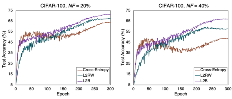
Figure 2: Test set accuracy versus the number of epochs on CIFAR-100 under the noise fraction of 20% and 40%.

Generalization to real-world noisy labels.

We test L2B on Clothing 1M [38], a large-scale dataset with real-world noisy labels. To further illustrate the effectiveness of our approach, we compare with: 1) Tanaka et al. [31], 2) MLNT [17], 3) MW-Net [30], 4) GLC [10], and 5) MLC [47] using the same validation and testing splits provided by the benchmark. The results of all competitors are reported from [47]. As shown in Table 4, our L2B achieves an average performance of 77.5% accuracy from 3 independent runs with different random seeds, outperforming all competing methods on the Clothing 1M benchmark.

Table 4: Comparison with state-of-the-art methods in test accuracy (%) under real-world noise on Clothing 1M. Our results are reported from 3 independent runs with different random seeds. All other results are reported from [47].

Method	Tanaka	MLNT	MW-Net	GLC	MLC	L2B
	et al. [31]	[17]	[30]	[10]	[47]	(Ours)
Accuracy	72.2	73.5	73.7	73.7	75.8	$\textbf{77.5}\pm 0.2$

Generalization to medical image analysis.

Table 5 demonstrates the generalizability of our proposed L2B to medical image analysis [40]. Compared with 1) L2RW [28], which has also been applied to skin lesion classification/segmentation [40, 22] with noisy supervision; 2) Distillation [19]; 3) Mixup [45]; and 4) Bootsrapping [27], our method achieves better results under all different noise levels.

Table 5: Comparison with different methods in test accuracy (%) on ISIC with symmetric noise.

Method	20% NF	30% NF	40% NF	50% NF
Cross-Entropy	79.4	77.5	75.3	73.7
Bootstrapping [27]	80.8	77.7	75.7	74.8
Distillation [19]	80.1	78.8	76.8	74.4
Mixup [45]	80.2	77.9	76.8	74.9
L2RW [28]	80.1	77.7	76.3	74.1
L2B (Ours)	81.1	80.2	78.6	76.8

Stability of experimental results.

We repeated the experiments 5 times with different random seeds for network initialization and label noise generation, and report mean $\pm$ standard deviation under different experimental settings. As can be seen from Table 6, with different noise fractions and datasets, the standard deviation among the 5 runs are consistently less that $0.5\%$.

Table 6: Multiple-runs experiments under the noise fraction of 20% NF and 40% NF.

Datasets	20% NF	40 % NF
CIFAR-10	91.99$\pm$ 0.10	89.39$\pm$ 0.22
CIFAR-100	71.78 $\pm$ 0.38	67.23 $\pm$ 0.33
ISIC 2019	81.16 $\pm$ 0.29	78.26 $\pm$ 0.45

4.4 Ablation Study

On the importance of $\boldsymbol{\alpha},\boldsymbol{\beta}$.

To understand why our proposed new learning objective can outperform previous meta-learning-based instance reweighting methods, we conduct the following analysis to understand the importance of hyper-parameter $\boldsymbol{\alpha}$ and $\boldsymbol{\beta}$ in our method. Specifically, we set $\boldsymbol{\alpha}=\boldsymbol{0}$ and $\boldsymbol{\beta}=\boldsymbol{0}$ respectively to investigate the importance of each loss term in Eq. (3). In addition, we also show how the restriction of $\alpha_{i}+\beta_{i}=1$ (Eq. (2)) would deteriorate our model performance as follows.

• $\boldsymbol{\alpha}=\boldsymbol{0}$. As shown in Table 7, in this case, the performance even decreases compared with the baseline approach. This is due to that when only pseudo-labels are included in the loss computation, the error which occurs in the initial pseudo-label will be reinforced by the network during the following iterations.

• $\boldsymbol{\beta}=\boldsymbol{0}$. From Eq. (3), we can see that setting $\boldsymbol{\beta}$ as $\boldsymbol{0}$ is essentially equivalent to the baseline meta-learning-based instance reweighting method L2RW [28]. In this case, the performance is largely improved compared to the baseline, but still inferior to our method, which jointly optimizes $\boldsymbol{\alpha}$ and $\boldsymbol{\beta}$.

• $\boldsymbol{\alpha}+\boldsymbol{\beta}=\boldsymbol{1}$. We also investigate whether the restriction of $\boldsymbol{\alpha}+\boldsymbol{\beta}=\boldsymbol{1}$ is required for obtaining optimal weights during the meta-update, as in [46]. As shown in Table 7, L2B ($\boldsymbol{\alpha},\boldsymbol{\beta}\geq\boldsymbol{0}$) consistently achieves superior results than L2B ($\boldsymbol{\alpha}+\boldsymbol{\beta}=\boldsymbol{1}$) under different noise levels on CIFAR-100. The reason may be the latter is only reweighting different loss terms, whereas the former not only explores the optimal combination between the two loss terms but also jointly adjusts the contribution of different training samples.

Table 7: Ablation study under the noise fraction of 20% and 40%. L2B ($\boldsymbol{\alpha},\boldsymbol{\beta}\geq\boldsymbol{0}$) consistently achieves superior results to L2B ($\boldsymbol{\alpha}+\boldsymbol{\beta}=\boldsymbol{1}$) under different noise levels on CIFAR-100.

Method	20% NF	40% NF
Cross-Entropy	59.6	49.2
$\boldsymbol{\alpha}=\boldsymbol{0}$	55.7	47.1
$\boldsymbol{\beta}=\boldsymbol{0}$	63.2	57.5
$\boldsymbol{\alpha}+\boldsymbol{\beta}=\boldsymbol{1}$	64.8	59.1
$\boldsymbol{\alpha},\boldsymbol{\beta}\geq\boldsymbol{0}$	71.8	67.3

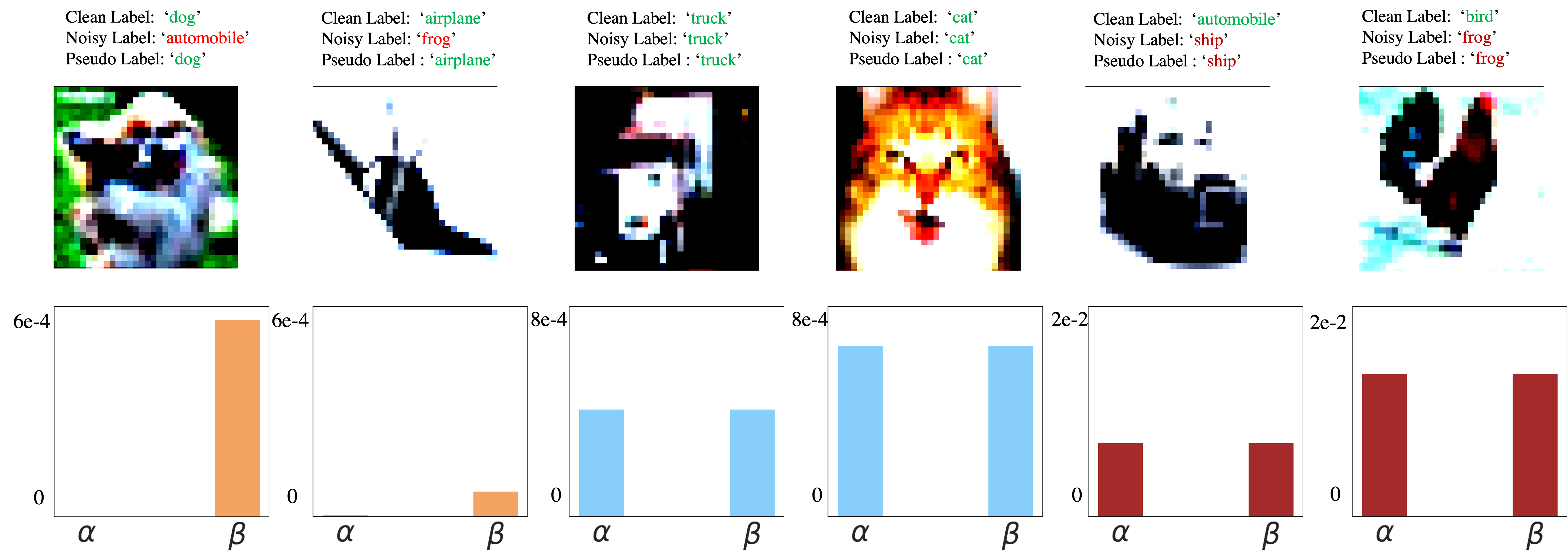
Figure 3: Examples of $\alpha$ and $\beta$ on CIFAR-10 with asymmetric noise fraction of 20%. When the estimated pseudo label is of high-quality, i.e., the pseudo label is different from the noisy label but equal to the clean label, our model will automatically assign a much higher weight to $\beta$ than to $\alpha$ for corrupted training samples. When the pseudo label is equal to the noisy label (i.e., the two loss terms are equal to each other), $\alpha$ and $\beta$ are almost identical.

We also demonstrate a set of qualitative examples to illustrate how our proposed L2B benefits from the joint instance and label reweighting paradigm. In Figure 3, we can see that when the estimated pseudo label is of high-quality, i.e., the pseudo label is different from the noisy label but equal to the clean label, our model will automatically assign a much higher weight to $\beta$ for corrupted training samples. On the contrary, $\alpha$ can be near zero in this case. This indicates that our L2B algorithm will pay more attention to the pseudo label than the real noisy label when computing the losses. In addition, we also show several cases where the pseudo label is equal to the noisy label, where we can see that $\alpha$ and $\beta$ are almost identical under this circumstance since the two losses are of the same value. Note that the relatively small values of $\alpha$ and $\beta$ are due to that we use a large batch size (i.e., 512) for CIFAR-10 experiments. By normalizing the weights in each training batch (see Eq. (9)), the value of $\alpha$ and $\beta$ can be on the scale of $10^{-4}$.

Parameter normalization.

We note that the normalization of $\boldsymbol{\alpha}$ and $\boldsymbol{\beta}$ is one key component for accelerating the training process. However, we observe that different normalization methods of $\boldsymbol{\alpha}$ and $\boldsymbol{\beta}$ behave quite differently for different datasets. To further investigate this, we apply the following normalization functions to each $\alpha_{i}$ and $\beta_{i}$ on ISIC2019, CIFAR-100 and Clothing 1M: 1) Eq. (9) as in [28], 2) Sigmoid function,

$$\alpha_{t,i}=\frac{1}{1+e^{-\alpha_{t,i}}},\ \beta_{t,i}=\frac{1}{1+e^{-\beta_{t,i}}},$$ (13)

and 3) Softmax function,

$$\alpha_{t,i}=\frac{e^{\alpha_{t,i}/\tau}}{\sum_{i}^{n}e^{\alpha_{t,i}/\tau}+e^{\beta_{t,i}/\tau}},\ \beta_{t,i}=\frac{e^{\beta_{t,i}/\tau}}{\sum_{i}^{n}e^{\alpha_{t,i}/\tau}+e^{\beta_{t,i}/\tau}},$$ (14)

where $t$ stands for the training iteration and $\tau$ denotes the temperature parameter for scaling the weight distribution. $\tau$ is set as 10.0 when using the Softmax function for normalization. The comparison among these three different normalization methods is summarized in Figure 4 on ISIC2019 and CIFAR-100 datasets with 40% symmetric noise. We can see that while Eq. (9) achieves the best result on CIFAR-100, it yields large training instability on the ISIC2019 dataset. Changing the normalization function to Sigmoid and Softmax can make the training procedure much more stable on the ISIC2019 dataset.

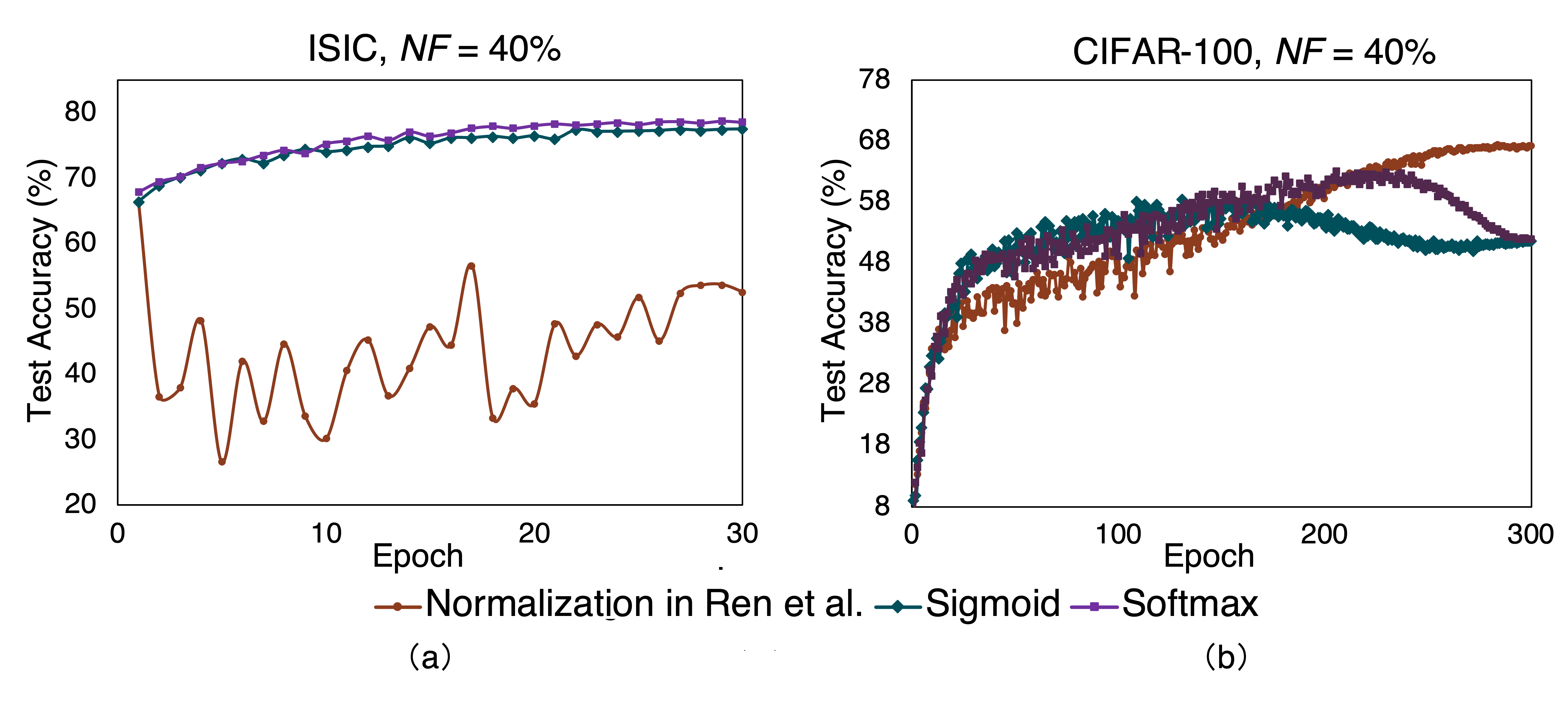
Figure 4: Comparison among different normalization functions (i.e., Eq. (9) as in  [28], Sigmoid function and Softmax function). (a) Testing accuracy curve with different normalization functions under 40% symmetric noise label on the ISIC dataset. (b) Testing accuracy curve with different normalization under 40% symmetric label noise on CIFAR-100.

In addition, we notice that Softmax (e.g., using the Softmax function with a temperature scaling of 10.0 instead of Eq. (9) to normalize $\boldsymbol{\alpha}$ and $\boldsymbol{\beta}$) slightly outperforms Sigmoid for ISIC2019. Future research should address how to develop a unified normalization function which can be generalizable for different learning tasks.

Comparison with meta-learning-based label correction.

One recent study [47] has proposed meta label correction to explicitly relabel the noisy examples via a meta-network. Unlike our L2B which conducts implicit relabeling via reweighting different loss components, this method uses a meta-model for explicit label correction. We re-implement the results with the public code by using PreActResNet-18 as the backbone network and the comparison results on CIFAR-10 are show in Table 8. We can see that our method consistently outperforms MLC for noise ratios ranging from 10% to 50% on CIFAR-10.

Table 8: Comparison with MLC  [47] in test accuracy (%) on CIFAR-10 with symmetric noise.

Method	10% NF	20% NF	30% NF	40% NF	50% NF
MLC	90.1	90.1	88.3	87.2	86.0
L2B (Ours)	93.6	92.2	90.7	89.9	88.5

Training cost.

We list our training time on CIFAR-10 compared with the previous meta-learning based instance reweighting methods, i.e., MLNT [17], L2RW [28], in Table 9. The training times are reported based on PreActResNet-18 on a single V100 GPU card. Our method L2B is directly built on top of L2RW, and our method (which applies a joint instance reweighting and label reweighting) incurs almost no extra training cost when using the same architecture and hardware conditions.

Table 9: Training time comparison of MLNT [17], L2RW [28] and L2B (Ours). Our L2B incurs almost no additional training cost when using the same architecture and hardware conditions.

MLNT [17]	L2RW [28]	L2B (Ours)
8.6 h	6.5h	6.5h

4.5 Discussion & Limitation

L2B is designed for building robust representation models, which is crucial for many real-world applications in healthcare, vision, etc. For example, high intra- and inter-physician variations are well-known in medical diagnostic tasks, which lead to erroneous labels that could derail our learning algorithms. L2B can help rectify such noisy data distributions and prevent potential overfitting during training and thus reduce the risking of medical errors.

This paper specifically focuses on the situation where a small clean validation set is accessible (e.g., Clothing 1M [38]). However, we do note that the extra validation dataset is not a requirement in meta-learning as we can use a subset of pseudo-labeled training data as the validation data [39]. How to properly select a high-quality pseudo-labeled set and how it affects the algorithm compared to the external validation set should be investigated in the future. Future study should also analyze the role of L2B in conjunction with other meta-learning-based instance reweighting methods such as MW-Net [30], and semi-supervised/self-supervised learning methods [16, 18], for furthering the performance.

5 Conclusion

In this paper, we present L2B, a simple and effective method for training noise-robust models. Concretely, we propose a novel and generic learning objective to enable joint reweighting of instances and labels for combating the label noise in deep representation learning. A meta process is employed to dynamically adjust the per-sample importance weight between real observed labels and pseudo-labels. Our L2B outperforms prior instance reweighting or label reweighting works under both synthetic and real-world noise with almost no extra cost.

Appendix

Appendix A Equivalence of the two learning objectives

We show that Eq. (3) is equivalent with Eq. (2) when $\forall i\ \alpha_{i}+\beta_{i}=1$. For convenience, we denote $y_{i}^{\text{real}},y_{i}^{\text{pseudo}},\mathcal{F}(x_{i},\theta)$ using $y_{i}^{r},y_{i}^{p},p_{i}$ respectively.

$$\alpha_{i}\mathcal{L}(p_{i},y_{i}^{r})+\beta_{i}\mathcal{L}(p_{i},y_{i}^{p})=\sum_{l=1}^{L}\alpha_{i}y_{i,l}^{r}\log p_{i,l}$$ (15)

$$+\beta_{i}y_{i,l}^{p}\log p_{i,l}=\sum_{l=1}^{L}(\alpha_{i}y_{i,l}^{r}+\beta_{i}y_{i,l}^{p})\log p_{i,l}$$ (16)

Due to that $\mathcal{L}(\cdot)$ is the cross-entropy loss, we have $\sum_{l=1}^{L}y_{i,l}^{r}=\sum_{l=1}^{L}y_{i,l}^{p}=1$. Then $\sum_{l=1}^{L}\alpha_{i}y_{i,l}^{r}+\beta_{i}y_{i,l}^{p}=\alpha_{i}+\beta_{i}$. So if $\alpha_{i}+\beta_{i}=1$, we have

$$\sum_{l=1}^{L}(\alpha_{i}y_{i,l}^{r}+\beta_{i}y_{i,l}^{p}) \log p_{i,l}=\mathcal{L}(p_{i},\alpha_{i}y_{i}^{r}+\beta_{i}y_{i}^{p})$$ (17)

$$=\mathcal{L}(p_{i},(1-\beta_{i})y_{i}^{r}+\beta_{i}y_{i}^{p})$$ (18)

Appendix B Gradient used for updating $\theta$

We derivative the update rule for $\boldsymbol{\alpha},\boldsymbol{\beta}$ in Eq. (10).

$$\alpha_{t,i} =-\eta\frac{\partial}{\partial\alpha_{i}}(\sum_{j=1}^{m}f_{j}^{v}(\hat{\theta}_{t+1}))\Big{|}_{\alpha_{i}=0}$$ (19)

$$=-\eta\sum_{j=1}^{m}\nabla f_{j}^{v}(\hat{\theta}_{t+1})^{T}\frac{\partial\hat{\theta}_{t+1}}{\partial\alpha_{i}}\Big{|}_{\alpha_{i}=0}$$ (20)

$$=-\eta\sum_{j=1}^{m}\nabla f_{j}^{v}(\hat{\theta}_{t+1})^{T}$$ (21)

$$\frac{\partial(\theta_{t}-\lambda\nabla(\sum_{k}\alpha_{k}\ f_{k}(\theta)+\beta_{k}\ g_{k}(\theta))\Big{|}_{\theta=\theta_{t}})}{\partial\alpha_{i}}\Big{|}_{\alpha_{i}=0}$$ (22)

$$=\eta\lambda\sum_{j=1}^{m}\nabla f_{j}^{v}(\theta_{t})^{T}\nabla f_{i}(\theta_{t})$$ (23)

$$\beta_{t,i} =-\eta\frac{\partial}{\partial\beta_{i}}(\sum_{j=1}^{m}f_{j}^{v}(\hat{\theta}_{t+1}))\Big{|}_{\beta_{i}=0}$$ (24)

$$=-\eta\sum_{j=1}^{m}\nabla f_{j}^{v}(\hat{\theta}_{t+1})^{T}\frac{\partial\hat{\theta}_{t+1}}{\partial\beta_{i}}\Big{|}_{\beta_{i}=0}$$ (25)

$$=-\eta\sum_{j=1}^{m}\nabla f_{j}^{v}(\hat{\theta}_{t+1})^{T}$$ (26)

$$\frac{\partial(\theta_{t}-\lambda\nabla(\sum_{k}\alpha_{k}\ g_{k}(\theta)+\beta_{k}\ g_{k}(\theta))\Big{|}_{\theta=\theta_{t}})}{\partial\beta_{i}}\Big{|}_{\beta_{i}=0}$$ (27)

$$=\eta\lambda\sum_{j=1}^{m}\nabla f_{j}^{v}(\theta_{t})^{T}\nabla g_{i}(\theta_{t})$$ (28)

Then $\theta_{t+1}$ can be calculated by Eq. (10) using the updated $\alpha_{t,i},\beta_{t,i}$.

Appendix C Convergence

This section provides the proof for covergence (Theorem 1)

Theorem.

Suppose that the training loss function $f,g$ have $\sigma$-bounded gradients and the validation loss $f^{v}$ is Lipschitz smooth with constant L. With a small enough learning rate $\lambda$, the validation loss monotonically decreases for any training batch $B$, namely,

$$G(\theta_{t+1})\leq G(\theta_{t}),$$ (29)

where $\theta_{t+1}$ is obtained using Eq. (10) and $G$ is the validation loss

$$G(\theta)=\frac{1}{M}\sum_{i=1}^{M}f_{i}^{v}(\theta),$$ (30)

Furthermore, Eq. (29) holds for all possible training batches only when the gradient of validation loss function becomes $0$ at some step $t$, namely, $G(\theta_{t+1})=G(\theta_{t})\ \forall B\Leftrightarrow\nabla G(\theta_{t})=0$

Proof. At each training step $t$, we pick a mini-batch $B$ from the union of training and validation data with $|B|=n$. From section B we can derivative $\theta_{t+1}$ as follows:

$$\theta_{t+1} =\theta_{t}-\lambda\sum_{i=1}^{n}(\alpha_{t,i}\nabla f_{i}(\theta_{t})+\beta_{t,i}\nabla g_{i}(\theta_{t}))$$ (31)

$$=\theta_{t}-\eta\lambda^{2}M\sum_{i=1}^{n}(\nabla G^{T}\nabla f_{i}\nabla f_{i}+\nabla G^{T}\nabla g_{i}\nabla g_{i})$$ (32)

We omit $\theta_{t}$ after every function for briefness and set $m$ in section B equals to $M$. Since $G(\theta)$ is Lipschitz-smooth, we have

$$G(\theta_{t+1})\leq G(\theta_{t})+\nabla G^{T}\Delta\theta+\frac{L}{2}||\Delta\theta||^{2}.$$ (33)

Then we show $\nabla G^{T}\Delta\theta+\frac{L}{2}||\Delta\theta||^{2}\leq 0$ with a small enough $\lambda$. Specifically,

$$\nabla G^{T}\Delta\theta=-\eta\lambda^{2}M\sum_{i}(\nabla G^{T}\nabla f_{i})^{2}+(\nabla G^{T}\nabla g_{i})^{2}.$$ (34)

Then since $f_{i},g_{i}$ have $\sigma$-bounded gradients, we have

$$\frac{L}{2}||\Delta\theta||^{2} \leq\frac{L\eta^{2}\lambda^{4}M^{2}}{2}\sum_{i}(\nabla G^{T}\nabla f_{i})^{2}||\nabla f_{i}||^{2}$$ (35)

$$+(\nabla G^{T}\nabla g_{i})^{2}||\nabla g_{i}||^{2}$$ (36)

$$\leq\frac{L\eta^{2}\lambda^{4}M^{2}\sigma^{2}}{2}\sum_{i}(\nabla G^{T}\nabla f_{i})^{2}+(\nabla G^{T}\nabla g_{i})^{2}$$ (37)

Then if $\lambda^{2}<\frac{2}{\eta\sigma^{2}ML}$,

$$\nabla G^{T}\Delta\theta+\frac{L}{2}||\Delta\theta||^{2} \leq(\frac{L\eta^{2}\lambda^{4}M^{2}\sigma^{2}}{2}-\eta\lambda^{2}M)$$ (38)

$$\sum_{i}(\nabla G^{T}\nabla f_{i})^{2}+(\nabla G^{T}\nabla g_{i})^{2}\leq 0.$$ (39)

Finally we prove $G(\theta_{t+1})=G(\theta_{t})\ \forall B\Leftrightarrow\nabla G(\theta_{t})=0$: If $\nabla G(\theta_{t})=0$, from section B we have $\alpha_{t,i}=\beta_{t,i}=0$, then $\theta_{t+1}=\theta_{t}$ and thus $G(\theta_{t+1})=G(\theta_{t})\ \forall B$. Otherwise, if $\nabla G(\theta_{t})\neq 0$, we have

$$0<||\nabla G||^{2}=\nabla G^{T}\nabla G=\frac{1}{M}\sum_{i=1}^{M}\nabla G^{T}\nabla f_{i}^{v},$$ (40)

which means there exists a $k$ such that $\nabla G^{T}\nabla f_{k}^{v}>0$. So for the mini-batch $B_{k}$ that contains this example, we have

$$G(\theta_{t+1})-G(\theta_{t}) \leq\nabla G^{T}\Delta\theta+\frac{L}{2}||\Delta\theta||^{2}$$ (41)

$$\leq(\frac{L\eta^{2}\lambda^{4}M^{2}\sigma^{2}}{2}-\eta\lambda^{2}M)$$ (42)

$$\sum_{i\in B}(\nabla G^{T}\nabla f_{i})^{2}+(\nabla G^{T}\nabla g_{i})^{2}$$ (43)

$$\leq(\frac{L\eta^{2}\lambda^{4}M^{2}\sigma^{2}}{2}-\eta\lambda^{2}M)\nabla G^{T}\nabla f_{k}^{v}$$ (44)

$$<0.$$ (45)

References

- [1] Eric Arazo, Diego Ortego, Paul Albert, Noel O’Connor, and Kevin McGuinness. Unsupervised label noise modeling and loss correction. In International Conference on Machine Learning, pages 312–321. PMLR, 2019.
- [2] Devansh Arpit, Stanislaw Jastrzkebski, Nicolas Ballas, David Krueger, Emmanuel Bengio, Maxinder S Kanwal, Tegan Maharaj, Asja Fischer, Aaron Courville, Yoshua Bengio, et al. A closer look at memorization in deep networks. In International Conference on Machine Learning, pages 233–242. PMLR, 2017.
- [3] Pengfei Chen, Ben Ben Liao, Guangyong Chen, and Shengyu Zhang. Understanding and utilizing deep neural networks trained with noisy labels. In International Conference on Machine Learning, pages 1062–1070. PMLR, 2019.
- [4] Tongtong Fang, Nan Lu, Gang Niu, and Masashi Sugiyama. Rethinking importance weighting for deep learning under distribution shift. In Neurips, 2020.
- [5] Benoît Frénay and Michel Verleysen. Classification in the presence of label noise: a survey. IEEE transactions on neural networks and learning systems, 25(5):845–869, 2013.
- [6] Jacob Goldberger and Ehud Ben-Reuven. Training deep neural-networks using a noise adaptation layer. In ICLR, 2017.
- [7] Bo Han, Quanming Yao, Xingrui Yu, Gang Niu, Miao Xu, Weihua Hu, Ivor Tsang, and Masashi Sugiyama. Co-teaching: Robust training of deep neural networks with extremely noisy labels. In International Conference on Machine Learning, 2018.
- [8] Jiangfan Han, Ping Luo, and Xiaogang Wang. Deep self-learning from noisy labels. In Proceedings of the IEEE/CVF International Conference on Computer Vision, pages 5138–5147, 2019.
- [9] Kaiming He, Xiangyu Zhang, Shaoqing Ren, and Jian Sun. Identity mappings in deep residual networks. In European conference on computer vision, pages 630–645. Springer, 2016.
- [10] Dan Hendrycks, Mantas Mazeika, Duncan Wilson, and Kevin Gimpel. Using trusted data to train deep networks on labels corrupted by severe noise. In Advances in Neural Information Processing Systems, 2018.
- [11] Lu Jiang, Zhengyuan Zhou, Thomas Leung, Li-Jia Li, and Li Fei-Fei. Mentornet: Learning data-driven curriculum for very deep neural networks on corrupted labels. In International Conference on Machine Learning, pages 2304–2313. PMLR, 2018.
- [12] Youngdong Kim, Junho Yim, Juseung Yun, and Junmo Kim. Nlnl: Negative learning for noisy labels. In Proceedings of the IEEE/CVF International Conference on Computer Vision, pages 101–110, 2019.
- [13] Youngdong Kim, Juseung Yun, Hyounguk Shon, and Junmo Kim. Joint negative and positive learning for noisy labels. In Proceedings of the IEEE/CVF Conference on Computer Vision and Pattern Recognition (CVPR), pages 9442–9451, June 2021.
- [14] Dong-Hyun Lee et al. Pseudo-label: The simple and efficient semi-supervised learning method for deep neural networks. In ICML Workshop on challenges in representation learning, 2013.
- [15] Kuang-Huei Lee, Xiaodong He, Lei Zhang, and Linjun Yang. Cleannet: Transfer learning for scalable image classifier training with label noise. In Proceedings of the IEEE Conference on Computer Vision and Pattern Recognition, pages 5447–5456, 2018.
- [16] Junnan Li, Richard Socher, and Steven CH Hoi. Dividemix: Learning with noisy labels as semi-supervised learning. In ICLR, 2020.
- [17] Junnan Li, Yongkang Wong, Qi Zhao, and Mohan S Kankanhalli. Learning to learn from noisy labeled data. In Proceedings of the IEEE/CVF Conference on Computer Vision and Pattern Recognition, pages 5051–5059, 2019.
- [18] Junnan Li, Caiming Xiong, and Steven C.H. Hoi. Learning from noisy data with robust representation learning. In Proceedings of the IEEE/CVF International Conference on Computer Vision (ICCV), pages 9485–9494, October 2021.
- [19] Yuncheng Li, Jianchao Yang, Yale Song, Liangliang Cao, Jiebo Luo, and Li-Jia Li. Learning from noisy labels with distillation. In Proceedings of the IEEE International Conference on Computer Vision, pages 1910–1918, 2017.
- [20] Sheng Liu, Jonathan Niles-Weed, Narges Razavian, and Carlos Fernandez-Granda. Early-learning regularization prevents memorization of noisy labels. Advances in neural information processing systems, 33:20331–20342, 2020.
- [21] Tongliang Liu and Dacheng Tao. Classification with noisy labels by importance reweighting. IEEE Transactions on pattern analysis and machine intelligence, 38(3):447–461, 2015.
- [22] Zahra Mirikharaji, Yiqi Yan, and Ghassan Hamarneh. Learning to segment skin lesions from noisy annotations. In Domain Adaptation and Representation Transfer and Medical Image Learning with Less Labels and Imperfect Data, pages 207–215. Springer, 2019.
- [23] Nagarajan Natarajan, Inderjit S Dhillon, Pradeep Ravikumar, and Ambuj Tewari. Learning with noisy labels. In NIPS, volume 26, pages 1196–1204, 2013.
- [24] David F Nettleton, Albert Orriols-Puig, and Albert Fornells. A study of the effect of different types of noise on the precision of supervised learning techniques. Artificial intelligence review, 33(4):275–306, 2010.
- [25] Diego Ortego, Eric Arazo, Paul Albert, Noel E. O’Connor, and Kevin McGuinness. Multi-objective interpolation training for robustness to label noise. In Proceedings of the IEEE/CVF Conference on Computer Vision and Pattern Recognition (CVPR), pages 6606–6615, June 2021.
- [26] Giorgio Patrini, Alessandro Rozza, Aditya Krishna Menon, Richard Nock, and Lizhen Qu. Making deep neural networks robust to label noise: A loss correction approach. In Proceedings of the IEEE Conference on Computer Vision and Pattern Recognition, pages 1944–1952, 2017.
- [27] Scott Reed, Honglak Lee, Dragomir Anguelov, Christian Szegedy, Dumitru Erhan, and Andrew Rabinovich. Training deep neural networks on noisy labels with bootstrapping. arXiv preprint arXiv:1412.6596, 2014.
- [28] Mengye Ren, Wenyuan Zeng, Bin Yang, and Raquel Urtasun. Learning to reweight examples for robust deep learning. In International Conference on Machine Learning, pages 4334–4343. PMLR, 2018.
- [29] Yanyao Shen and Sujay Sanghavi. Learning with bad training data via iterative trimmed loss minimization. In International Conference on Machine Learning, pages 5739–5748. PMLR, 2019.
- [30] Jun Shu, Qi Xie, Lixuan Yi, Qian Zhao, Sanping Zhou, Zongben Xu, and Deyu Meng. Meta-weight-net: Learning an explicit mapping for sample weighting. In Advances in Neural Information Processing Systems, 2019.
- [31] Daiki Tanaka, Daiki Ikami, Toshihiko Yamasaki, and Kiyoharu Aizawa. Joint optimization framework for learning with noisy labels. In Proceedings of the IEEE Conference on Computer Vision and Pattern Recognition, pages 5552–5560, 2018.
- [32] Arash Vahdat. Toward robustness against label noise in training deep discriminative neural networks. In NIPS, 2017.
- [33] Andreas Veit, Neil Alldrin, Gal Chechik, Ivan Krasin, Abhinav Gupta, and Serge Belongie. Learning from noisy large-scale datasets with minimal supervision. In Proceedings of the IEEE conference on computer vision and pattern recognition, pages 839–847, 2017.
- [34] Xiaosong Wang, Ziyue Xu, Dong Yang, Leo Tam, Holger Roth, and Daguang Xu. Learning image labels on-the-fly for training robust classification models. arXiv preprint arXiv:2009.10325, 2020.
- [35] Hongxin Wei, Lei Feng, Xiangyu Chen, and Bo An. Combating noisy labels by agreement: A joint training method with co-regularization. In IEEE/CVF Conference on Computer Vision and Pattern Recognition (CVPR), June 2020.
- [36] Zhi-Fan Wu, Tong Wei, Jianwen Jiang, Chaojie Mao, Mingqian Tang, and Yu-Feng Li. Ngc: A unified framework for learning with open-world noisy data. In Proceedings of the IEEE/CVF International Conference on Computer Vision, pages 62–71, 2021.
- [37] Xiaobo Xia, Tongliang Liu, Nannan Wang, Bo Han, Chen Gong, Gang Niu, and Masashi Sugiyama. Are anchor points really indispensable in label-noise learning? In Neurips, 2019.
- [38] Tong Xiao, Tian Xia, Yi Yang, Chang Huang, and Xiaogang Wang. Learning from massive noisy labeled data for image classification. In Proceedings of the IEEE conference on computer vision and pattern recognition, pages 2691–2699, 2015.
- [39] Youjiang Xu, Linchao Zhu, Lu Jiang, and Yi Yang. Faster meta update strategy for noise-robust deep learning. In Proceedings of the IEEE/CVF Conference on Computer Vision and Pattern Recognition, pages 144–153, 2021.
- [40] Cheng Xue, Qi Dou, Xueying Shi, Hao Chen, and Pheng-Ann Heng. Robust learning at noisy labeled medical images: Applied to skin lesion classification. In 2019 IEEE 16th International Symposium on Biomedical Imaging (ISBI 2019), pages 1280–1283. IEEE, 2019.
- [41] Yazhou Yao, Zeren Sun, Chuanyi Zhang, Fumin Shen, Qi Wu, Jian Zhang, and Zhenmin Tang. Jo-src: A contrastive approach for combating noisy labels. In Proceedings of the IEEE/CVF Conference on Computer Vision and Pattern Recognition (CVPR), pages 5192–5201, June 2021.
- [42] Yu Yao, Tongliang Liu, Bo Han, Mingming Gong, Jiankang Deng, Gang Niu, and Masashi Sugiyama. Dual t: Reducing estimation error for transition matrix in label-noise learning. In Neurips, 2020.
- [43] Kun Yi and Jianxin Wu. Probabilistic end-to-end noise correction for learning with noisy labels. In Proceedings of the IEEE/CVF Conference on Computer Vision and Pattern Recognition, pages 7017–7025, 2019.
- [44] Xingrui Yu, Bo Han, Jiangchao Yao, Gang Niu, Ivor Tsang, and Masashi Sugiyama. How does disagreement help generalization against label corruption? In International Conference on Machine Learning, pages 7164–7173. PMLR, 2019.
- [45] Hongyi Zhang, Moustapha Cisse, Yann N Dauphin, and David Lopez-Paz. mixup: Beyond empirical risk minimization. In ICLR, 2018.
- [46] Zizhao Zhang, Han Zhang, Sercan O Arik, Honglak Lee, and Tomas Pfister. Distilling effective supervision from severe label noise. In Proceedings of the IEEE/CVF Conference on Computer Vision and Pattern Recognition, pages 9294–9303, 2020.
- [47] Guoqing Zheng, Ahmed Hassan Awadallah, and Susan Dumais. Meta label correction for noisy label learning. In Proceedings of the 35th AAAI Conference on Artificial Intelligence, 2021.
- [48] Xiong Zhou, Xianming Liu, Chenyang Wang, Deming Zhai, Junjun Jiang, and Xiangyang Ji. Learning with noisy labels via sparse regularization. In Proceedings of the IEEE/CVF International Conference on Computer Vision, pages 72–81, 2021.
- [49] Zhaowei Zhu, Tongliang Liu, and Yang Liu. A second-order approach to learning with instance-dependent label noise. In Proceedings of the IEEE/CVF Conference on Computer Vision and Pattern Recognition (CVPR), pages 10113–10123, June 2021.