Multivariate cluster point process to quantify and explore multi-entity configurations: Application to biofilm image data

Abstract

[Abstract]Clusters of similar or dissimilar objects are encountered in many fields. Frequently used approaches treat each cluster’s central object as latent. Yet, often objects of one or more types cluster around objects of another type. Such arrangements are common in biomedical images of cells, in which nearby cell types likely interact. Quantifying spatial relationships may elucidate biological mechanisms. Parent-offspring statistical frameworks can be usefully applied even when central objects (“parents”) differ from peripheral ones (“offspring”). We propose the novel multivariate cluster point process (MCPP) to quantify multi-object (e.g., multi-cellular) arrangements. Unlike commonly used approaches, the MCPP exploits locations of the central parent object in clusters. It accounts for possibly multilayered, multivariate clustering. The model formulation requires specification of which object types function as cluster centers and which reside peripherally. If such information is unknown, the relative roles of object types may be explored by comparing fit of different models via the deviance information criterion (DIC). In simulated data, we compared a series of models’ DIC; the MCPP correctly identified simulated relationships. It also produced more accurate and precise parameter estimates than the classical univariate Neyman-Scott process model. We also used the MCPP to quantify proposed configurations and explore new ones in human dental plaque biofilm image data. MCPP models quantified simultaneous clustering of Streptococcus and Porphyromonas around Corynebacterium and of Pasteurellaceae around Streptococcus and successfully captured hypothesized structures for all taxa. Further exploration suggested the presence of clustering between Fusobacterium and Leptotrichia, a previously unreported relationship.

, , , , , ,and (2024), Multivariate cluster point process to quantify and explore multi-entity configurations: Application to biofilm image data, Stat. In Medicine, 2024;00:1–6.

1 Introduction

Instances abound in nature where one type of object is dispersed around another type of object. At interplanetary and field ecologic scales, respectively, radio galaxies ¹, ² and forest songbirds ³ exemplify spatial clustering. At microscopic scales, among human cells and single-celled organisms, such arrangements are common. For example, hair cell development in the inner ear depends on surrounding support cells ⁴, neurons generally require various adjacent support cells ⁵, granulomatous lesions of the lung exhibit concentric rings of different cell types ⁶, and platelets aggregate around red blood cells during clot formation, which can also involve other cell types. To describe and quantify such arrangements, we have developed a new multivariate cluster point process model (MCPP). We also developed a procedure for using the MCPP to explore possible clustering relationships not known a priori. In human dental plaque biofilm, spherical Streptococcus cells often cluster around the ends of filamentous Corynebacterium cells ⁷, ⁸. These corncob-like arrangements have been observed for decades and likely hold clues about microbial interactions that can affect human health. We assessed performance of the MCPP through simulations and by application to dental plaque biofilm image data.

Most biofilm image analysis approaches have focused on macro-level structural characteristics or derived features, such as biofilm volume, thickness, or surface roughness ⁹, ¹⁰. Less commonly, spatial point process models have been used to analyze the spatial patterning of microbial cells: how cells of one taxonomic class (or taxon) are distributed in relation to other cells of the same or different taxa. However, standard point process models, such as the log-Gaussian Cox process model ¹¹, do not account for the complex spatial clustering arrangements often present in biofilm images. Methods that can account for such complexity are needed to quantify visible arrangements and to explore and quantify spatially dependent arrangements that, unlike the “corncobs", are not visually discernable. Quantification, in turn, would allow benchmarking and hypothesis testing, such as for comparing effects of an antibacterial treatment on biofilm architecture.

The Neyman-Scott process model (NSP) ¹² is a classic statistical model used to quantify spatially dependent clustering relationships, most often applied to actual parents and offspring (such as trees in a forest). In this approach, locations of the central object in each cluster are treated as latent, in part because in a cluster comprising similar objects (such as a grove of trees or a school of fish), it may be impossible to identify any true parent individuals. In contrast, in corncob arrangements in dental plaque biofilm, the locations of the central cells are often known. Though reasonable for within-taxon clustering, naïve application of the NSP model to investigate between-taxon relationships is inappropriate because it ignores the taxon in the center of the clusters.

Corncob arrangements in dental plaque biofilm have other characteristics that preclude direct application of the NSP model or the related shot noise Cox process model ¹³. First, the “parent” (i.e., central) and “offspring” (i.e., peripheral) cells are of different bacterial taxa, thus requiring a multivariate extension of univariate approaches. Though others have considered point process models for multi-type spatial data ¹⁴, ¹¹, ¹⁵, ¹⁶, we are unaware of any work addressing more complex clustering arrangements as a specific focus of model development. Second, the corncob arrangements sometimes include multiple “offspring” taxa in that both Streptococcus and Porphyromonas are observed around Corynebacterium “parents.” Existing multivariate cluster point process models ¹⁷, ¹⁸ Bull. astr. Inst. Czechosl.can not model the taxon in the cluster center and have no scope to enforce multiple offspring taxa’s having the same parent taxon.

¹⁹ propose a multivariate clustering process model that permits multiple types of offspring to be clustered around the center. In the proposed configuration, however, any offspring can be affected by all potential cluster centers. Thus these models fail to exploit biological knowledge about which taxa are parents to which other offspring taxa. Further, parent processes are considered as fixed, known quantities and are not explicitly modeled. To our knowledge, existing approaches fail to address a third challenge, that the corncobs can be multilayered in nature (e.g., Figure 1). Fourth, the corncob arrangements themselves are part of a more complexly organized community that includes other taxa unrelated to the arrangements. None of the aforementioned methods address this challenge. Fifth, clustering configurations are not always known a priori. When configurations are known, the analysis goal might be to quantify them; in other instances the goal might be to explore the possible existence of clustering relationships.

The primary innovation of the proposed MCPP model is that it exploits the known locations of central objects in clusters. It also addresses the above-described challenges together. Specifically, it can simultaneously quantify multivariate and multilayered clustering and inter-process relationships. The MCPP is flexible in that it can simultaneously model clustered and non-clustered processes and can be applied in multivariate (multi-taxon) or univariate (individual taxon) contexts. It may seem restrictive that fitting the MCPP model requires specification of which objects are central to clusters and which peripherally located. We demonstrate that the MCPP can also be used to explore and infer the presence of newly proposed relationships by comparing model fit via the deviance information criterion (DIC). In this paper, we describe the model in detail, evaluate its performance through simulation studies, and demonstrate the feasibility of applying the model to both real and synthetic datasets.

Figure 1: A multi-layered parent-offspring structure. The green dots behave as offspring to the pink dot while the orange dots behave as offspring to the green dots

Figure 2: (a) A biofilm image of a dental plaque sample from from a human donor: RGB image - taxa relevant to the multilayered concob arrangements are Corynebacterium (Pink), Streptococcus (Green), Porphyromonas (Blue) and Pasteurellaceae (Orange); (b) post-segmentation spatial locations of the centroids of cells identified via genus-specific probes, as indicated

2 Microbiome Biofilm Image Data from Dental Plaque Samples

In this section, we present image data that motivate development of the method and that we analyzed by applying the MCPP. These data and their collection methods and processing have been described in detail elsewhere ⁸. Briefly, dental plaque samples were collected, embedded in methacrylate, sectioned, and subjected to multi-spectral fluorescence in situ hybridization (FISH) imaging. Multiple genus- and family-level probes were applied simultaneously to identify nine taxa. The near-universal probe Eub338 targeting most bacteria was also included (Figure 2(a)). We performed segmentation of the biofilm image in FIJI ²⁰ by applying a $3\times 3$ median filter and the “Auto Local" thresholding function with the Bersen method. Spatial coordinate information for each cell’s centroid was generated by applying the “Analyze Particles" function with size filter of 0.5 $\mu m$ diameter in FIJI (Figure 2(b)).

The sampled image is representative of similar samples from the same and other donors without active tooth decay (not shown). Filamentous Corynebacterium cells (Figure 3, pink) are common. Members of this genus are now believed to help establish the “healthy" dental microbiota, providing a scaffold around which other community members assemble. Some Streptococcus (Figure 3, green) and/or Porphyromonas (Figure 3, blue) cells surround the tips of Corynebacterium filaments ⁸. Adding another layer and further complexity, Pasteurellaceae cells (Figure 3, orange) sometimes surround Streptococcus cells ⁸, ²¹. As outlined in Section 1, these arrangements allow Streptococcus to serve as either parent, offspring, or both in the same cluster. Other taxa scatter seemingly homogeneously and may have additional spatial relationships with Corynebacterium, Streptococcus, Porphyromonas, or Pasteurellaceae (Supplementary Materials, Section B). Below, we demonstrate a procedure to explore previously undescribed patterns among these other taxa.

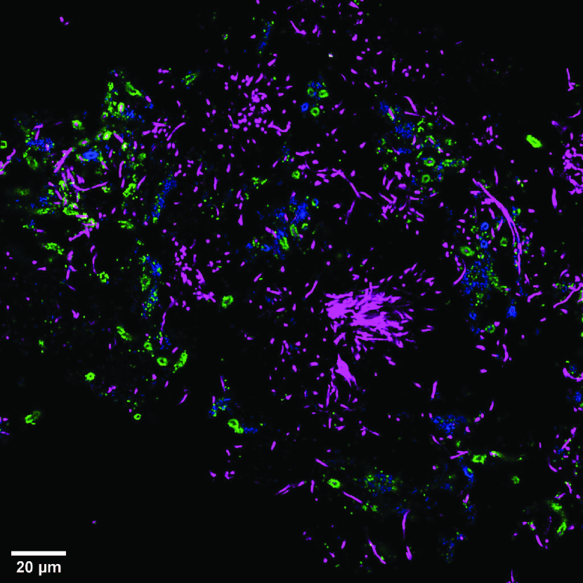
((a))

((b))

((c))

((d))

Figure 3: (a) The same image as in Figure 2, displaying channels corresponding to Corynebacterium (Pink), Streptococcus (green) and Porphyromonas (Blue); (b) cartoon depicting various corncob structures visible in the image. The corncob structures are present in areas of the image corresponding to the tip of the Corynebacterium. At the center of the dense clump of Corynebacterium in (a), no corncobs are observed; (c) The same image as in Figure 2, displaying channels corresponding to Pasteurellaceae (Orange) and Streptococcus (Green); and (d) a cartoon image illustrating the clustering of Pasteurellaceae around Streptococcus. Hiding the pink Corynebacterium channels highlights the outer layer in the multilayer arrangements. For other examples of biofilm images with corncob structures in which both Streptococcus and Porphyromonas cells cluster around the same Corynebacterium cell, see Supplemental Figure S2, panel C, in Mark Welch et al. (2016).

3 Multivariate Cluster Point Process Model

We consider a multivariate process $Y$ to be a collection of processes $Y_{i}\,,\ i=1,\ldots,m$, at location $\mbox{\bf s}\in\mathcal{W}\subset\mbox{${\mathbb{R}^{2}}$}$, where each component $Y_{i}$ is a Poisson process characterized by an intensity function $\lambda_{i}(\mbox{\bf s})$ and $\mathcal{W}$, the observation window. In application to the biofilm sample, each $Y_{i}$ captures the spatial distribution of the $i$-th taxon.

3.1 Model formulations

Suppose that $Y_{1},\ldots,Y_{p}$, are homogeneous Poisson processes (HPP) with intensities $\lambda_{v}^{C}$ for $v=1,\ldots,p~{}(<m)$, and they serve only as parent processes (“C" signifies central objects, or parents). Then we consider the $q\,\ (\leq m-p)$ processes, $Y_{p+1},\ldots,Y_{p+q}$, that behave as offspring processes. Each offspring process is assumed to have one parent process. Let $C_{l}$ for $l=p+1,\ldots,p+q$ denote the corresponding parent process for offspring process $Y_{l}$ with the following properties:

1. If offspring processes $Y_{l}$ and $Y_{l^{\prime}}\,,\ l\neq l^{\prime}$ share a parent process, then $C_{l}=C_{l^{\prime}}$;

2. If an offspring process $Y_{j}$ serves as a parent process for another offspring process $Y_{l}$ for some $l$ and $j=p+1,\ldots,p+q$, then $C_{l}=Y_{j}$.

We assume that the offspring points are distributed around parent point $\mbox{\bf c}\in C_{l}\,,\ l\in\{p+1,\ldots,p+q\}$ according to the rule $\alpha_{l}k_{l}(\cdot-\mbox{\bf c},h_{l})$, where $\alpha_{l}$ is the average number of offspring per parent, $k_{l}(\cdot,\cdot)$ is a kernel (e.g. Gaussian, uniform or Cauchy), and $h_{l}$ is a bandwidth parameter that controls the distance between the parent and its offspring locations for the $l$-th offspring process ²². The remaining $m-p-q$ types (e.g. taxa) that are unrelated to multilayered arrangements are modeled as HPP with intensities $\lambda_{j}$ for $j=p+q+1,\ldots,m$. Therefore, under the proposed specification, the intensity functions for the various processes are

$$\begin{split}\lambda_{v}(\mbox{\bf s})&=\lambda_{v}^{C}\,,\ v=1,\ldots,p\,,\ \lambda_{l}(\mbox{\bf s})=\alpha_{l}\sum_{\mbox{\bf c}_{l}\in C_{l}}k_{l}(\mbox{\bf s}-\mbox{\bf c}_{l},h_{l})\,,\ l=p+1,\ldots,p+q,\\ \lambda_{j}(\mbox{\bf s})&=\lambda_{j}\,,\ j=p+q+1,\ldots,m.\end{split}$$ (1)

Since the different processes are assumed to be conditionally independent of each other, the log-likelihood as a function of the unknown parameters, $\theta$ = $\big{\{}$$\alpha_{p+1}$, $\ldots$ ,$\alpha_{p+q}$,$h_{p+1}$, $\ldots$ , $h_{p+q}$, $\lambda_{1}^{C}$, $\ldots$ ,$\lambda_{p}^{C}$, $\lambda_{p+q+1}$, $\ldots$ ,$\lambda_{m}$$\big{\}}$, is given by

$$\begin{split}l(Y|\mbox{\boldmath$\theta$})&\propto\lvert\mathcal{W}\rvert-\sum_{v=1}^{p}\lvert\mathcal{W}\rvert\lambda^{C}_{v}-\sum_{l=p+1}^{p+q}\alpha_{l}\sum_{\mbox{\bf c}_{l}\in C_{l}}\int_{\mathcal{W}}k_{l}(\mbox{\bf u}-\mbox{\bf c}_{l},h_{l})\text{d}\mbox{\bf u}-\sum_{j=p+q+1}^{m}\lvert\mathcal{W}\rvert\lambda_{j}\\ &+\sum_{v=1}^{p}n_{v}\log\lambda^{C}_{v}+\sum_{l=p+1}^{p+q}\sum_{\mbox{\bf y}\in Y_{l}}\log\left(\alpha_{l}\sum_{\mbox{\bf c}_{l}\in C_{l}}k_{l}(\mbox{\bf y}-\mbox{\bf c}_{l},h_{l})\right)+\sum_{j=p+q+1}^{m}n_{j}\log\lambda_{j},\end{split}$$ (2)

where $\lvert\mathcal{W}\rvert$ is the area of $\mathcal{W}$, and $n_{i}$ denotes the number of observations from the $i$-th process in $\mathcal{W}$.

3.2 Quantities of interest

For a stationary point process, Ripley’s $K(r)$ function ²³ is defined as the expected number of neighbors located within distance $r$ from a typical point, divided by the intensity of the process. Since some of the processes being modeled are non-stationary, we shall use $K_{inhom}$ ²⁴, the inhomogeneous $K$-function. For either a homogeneous or inhomogeneous process $i$, we can estimate $K_{i}(r)$ by

$$\hat{K}_{i}(r)=\sum_{\mbox{\bf s},\mbox{\bf u}\in Y_{i}}\frac{\mathbb{I}(0<\lVert\mbox{\bf s}-\mbox{\bf u}\rVert\leq r)}{\lambda_{i}(\mbox{\bf s};\hat{\mbox{\boldmath$\theta$}}_{i})\lambda_{i}(\mbox{\bf u};\hat{\mbox{\boldmath$\theta$}}_{i})}w_{\mbox{\bf s},\mbox{\bf u}},$$ (3)

where $\hat{\mbox{\boldmath$\theta$}}_{i}$ is the set of estimated parameters that control process $i$, and $w_{\mbox{\bf s},\mbox{\bf u}}$ is the Ripley’s edge-correction factor ²⁵. For homogeneous point patterns, the estimate (3) is close to $\pi r^{2}$ for all values of $r$, and thus the estimated $K$-functions corresponding to $Y_{j}$, for $j=1,\ldots,p$, $p+q+1,\ldots,m$ should be close to $\pi r^{2}$. For inhomogeneous processes, the closed form expression is not evident, as is the case for processes $Y_{j}$ for $j=p+1,\ldots,p+q$.

By graphing the $K$-function, one can use it to assess homogeneity of processes. While it can thus be used to describe spatial patterns within a certain range, the $K$-function does not allow for quantitative validation of the point process models. Therefore, we interpret the MCPP model based on the individual model parameters, which, in turn, influence the estimated $K$-functions.

As outlined in Section 3.1, parameters of primary interest in the proposed model are the $\alpha_{l}$ and $h_{l}$ parameters, for $l=p+1,\ldots,p+q$. The offspring density parameter $\alpha_{l}$ corresponds to how densely the $l$-th process clusters around its parent process, with higher values indicating denser clustering. The bandwidth parameter, $h_{l}$ determines how tightly the $l$-th process clusters around its parent process. A value of $h_{l}>h_{0}$ may indicate no or negligible clustering between the $l$-th process and its supposed parent process, where $h_{0}$ is a predetermined threshold based on domain knowledge from experts. Interpretation of $h_{l}$ can change depending on choice of $k_{l}(\cdot,\cdot)$. For example, in a Gaussian or Cauchy kernel, $h_{l}$ can be thought of as a scaled average distance between the offspring and parent, whereas in a uniform kernel, it represents the maximum distance between the parent and its offspring. Regardless of $k_{l}(\cdot,\cdot)$, one can also interpret $h_{l}$ as a parameter that estimates the median distance between the parents and offsprings: $\frac{32}{27}h$, $\sqrt{5}h$ and $\frac{2}{3}h$ for Gaussian, Cauchy and uniform kernels respectively. These parameters provide additional quantitative information about the relationship between a clustered process and its parent process, quantities not captured by the $K(r)$ function.

3.3 Prior distributions and practical considerations

We outline priors for the unknown model parameters to complete the Bayesian specification of the MCPP model. Specifically, we consider the following priors:

$$\begin{split}\alpha_{l}&\stackrel{{\scriptstyle iid}}{{\sim}}\text{Gamma}(a_{Y},b_{Y})\,,\ h_{l}\stackrel{{\scriptstyle iid}}{{\sim}}\text{Half-Normal}(\sigma)\,,\ l=p+1,\ldots,p+q,\\ \lambda^{C}_{v}&\stackrel{{\scriptstyle iid}}{{\sim}}\text{Gamma}(a_{C},b_{C})\,,\ v=1,\ldots,p\,,\ \lambda_{j}\stackrel{{\scriptstyle iid}}{{\sim}}\text{Gamma}(a,b)\,,\ j=p+q+1,\ldots,m,\end{split}$$ (4)

where $\stackrel{{\scriptstyle iid}}{{\sim}}$ denotes independent and identically distributed, and ($a,b,a_{Y},b_{Y},a_{C},b_{C},\sigma$) are hyperparameters to be specified.

It is well appreciated that using a noninformative prior for spatial bandwidth or scale parameters is impossible due to numerical reasons, specifically, weak identifiability of the posterior distribution ²⁶, ²⁷, ²⁸. We use a half-normal prior for the bandwidth parameters $h_{l}$; ensuring the prior assigns mass to relatively small positive values, stabilizing the parameter estimation. Specifically, the value of hyperparameter $\sigma$ can be set such that the 99-th percentile of the half-normal prior corresponds to the maximum distance $d$ between a parent point and offspring points. This choice helps sensitize the proposed Bayesian framework to stronger clustering within a small radius, which is expected when, for example, cells of two bacterial taxa directly interact. In general, choosing the value of $d$ should depend on the context.

3.4 Computational scheme

Combining (2) and (4), the joint posterior density for the proposed MCPP model can be written as $\pi(\mbox{\boldmath$\theta$}|Y)\propto L(Y|\mbox{\boldmath$\theta$})\pi(\mbox{\boldmath$\theta$})$, where $\pi(\mbox{\boldmath$\theta$})$ is the product of all the individual prior densities. We then proceed to draw samples from the posterior distribution by using a Markov chain Monte Carlo (MCMC) algorithm. Conventional NSP-type approaches treat the number of parent points and their locations as random and thus require an additional reversible jump MCMC step to estimate the parameters associated with the latent parent process ²⁹, ²⁶. In contrast, the proposed framework exploits the fact that the parent processes are observed and proceeds without a complex birth-death-move algorithm. The components of $\theta$ can then be updated by Gibbs sampling (exploiting conjugacies in the full conditionals) or via Metropolis-Hastings steps (details in Section C of the Supplementary Material).

One practical challenge is that the integral term in (2) does not have a closed-form expression. Therefore, we use Monte Carlo methods to approximate the integral for computational efficiency. In practice, the expression $\int_{\mathcal{W}}k_{l}(\mbox{\bf u}-\mbox{\bf c}_{l},h_{l})\text{d}\mbox{\bf u}$ can be thought of as the probability of occurrence of $\mathbf{X}_{l}$ within the observation window $\mathcal{W}$, where $\mathbf{X}_{l}$ is a bivariate real-valued random variable with density $k_{l}(\cdot-\mbox{\bf c}_{l},h_{l})$. Furthermore, in the proposed framework with Thomas processes, $k_{l}(\cdot-\mbox{\bf c}_{l},h_{l})$ corresponds to a bivariate normal density function with mean $\mbox{\bf c}_{l}$ and covariance matrix $h_{l}^{2}\mathbf{I}$. In this case, we draw samples from the bivariate normal distribution and compute the average proportion of points that fall within $\mathcal{W}$, which serves as an approximation to the integral term in (2).

We further optimized the code by using the C language. An R package is available in the online repository at https://github.com/SumanM47/MCPP.git. The implementation of the model in the R package can generate 10,000 scans in 1.5 minutes for a dataset with ${\sim}150$ points from a single parent process with a total of ${\sim}750$ points from two offspring processes on a Dell Latitude 7210 laptop with i5 cores and 16 gigabytes of memory.

3.5 A metric to explore model configurations

Use of the MCPP model requires prespecification of parent-offspring arrangement. In practice, one may lack prior knowledge of intertaxon spatial clustering. One may suspect their existence, or one may simply seek to explore consistency of the data with one or more possible clustering arrangements. For this purpose, we propose a model validation method to identify a best-fitting model among a series of models specifying different possible clustering relationships. Specifically, we use the DIC ³⁰ to compare models involving different parent-offspring structures and/or different kernels for the distribution of offspring around the parent. For example, models could be fit such that A is assumed to cluster around B in model 1, C around D in model 2, and both in model 3. The model with the smallest DIC would be identified as the best fit. This model comparison process enables use of the MCPP as an exploratory tool. Newly proposed clustering arrangements can be quantified and evaluated for consistency with the data.

3.6 Goodness-of-fit

We also assess goodness-of-fit of the models by comparing the observed and estimated counts of different objects (in this case, taxa). Specifically, for the parent species, the estimated intensity parameter $\lambda^{C}_{v}$, $v=1,\ldots,p$, per unit area can be scaled by the area of the observation window. If the model is approximately correct, this quantity, $\lambda^{C}_{v}\lvert W\rvert$, should be close to the number of $v$-th parent cells counted in the observation window. For approximating the $l$-th offspring count, one can compute the posterior mean of $\alpha_{l}\sum_{\mbox{\bf c}\in C_{l}}\int_{W}k_{l}(\mbox{\bf u}-\mbox{\bf c},h_{l})d\mbox{\bf u}$ for $l=p+1,\ldots,p+q$. The integral term can be approximated by Monte Carlo methods as described in Section 3.4. This expression involves both the offspring density parameter and the bandwidth parameter and therefore helps validate the joint estimate of the $(\alpha_{l},h_{l})$ pair. In our example, $\lambda^{C}\lvert W\rvert$ should provide a good estimate of the number of Corynebacterium cells; and $\alpha_{2}\sum_{\mbox{\bf c}\in C_{2}}\int_{W}k_{2}(\mbox{\bf u}-\mbox{\bf c},h_{2})d\mbox{\bf u}$, $\alpha_{3}\sum_{\mbox{\bf c}\in C_{3}}\int_{W}k_{3}(\mbox{\bf u}-\mbox{\bf c},h_{3})d\mbox{\bf u}$ and $\alpha_{4}\sum_{\mbox{\bf c}\in C_{4}}\int_{W}k_{4}(\mbox{\bf u}-\mbox{\bf c},h_{4})d\mbox{\bf u}$ should be close to the observed number of Streptococcus clustered around Corynebacterium, the observed number of Porphyromonas clustered around Corynebacterium, and the observed number of Pasteurellaceae clustered around Streptococcus, respectively.

4 Simulation Studies

We performed two types of simulation studies to benchmark the performance of the method as an inference tool and as an exploratory tool. The first simulation study was designed to assess performance of the MCPP when the true parent-offspring relationships are known and to compare its performance to that of an existing method, the NSP. The second study was designed to assess the MCPP’s performance in ranking the fit of models parameterizing different proposed parent-offspring relationships and different kernels, and in identifying the best-fitting model. In both types of studies, we compared the estimated and true parameter values under the generating model.

4.1 Simulation I: Comparative performance for quantifying a prespecified configuration

4.1.1 Simulation set-up

For simplicity, the unit square was taken as the observation window. We generated data under the model outlined in Section 3, with $q=2$ offspring taxa B and C around the same parent taxon A, which was the only parent taxon ($p=1$). We considered twelve data scenarios (Supplementary Material Table S.1) that varied in terms of offspring density ($\alpha_{2}$, $\alpha_{3}$) being ‘Sparse’, ‘Dense’ or ‘Mixed’; bandwidth ($h_{2}$, $h_{3}$) being ‘Low’ or ‘High’; and presence or absence of a taxon spatially unrelated to the multilayered arrangement (hereinafter referred to as “unrelated" taxon). Throughout the scenarios, the intensity of the parent process ($\lambda_{1}^{C}$) and that of the process for the unrelated taxon ($\lambda_{4}$) were set to $150$ and $95$, respectively. For each of the twelve scenarios, we generated $100$ images, each analyzed as an independent dataset.

4.1.2 Analysis plan and hyperparameters

We applied the following approaches to each simulated dataset:

1. MCPP: Multi-offspring taxa (A as the parent of B or C) were jointly analyzed in one framework by using the MCPP.

2. NSP: Ignoring the parent taxon A, only offspring taxa B and C were analyzed separately (by necessity, with the NSP). We applied the method of minimum contrast ²⁷, by using the R package spatstat ³¹.

The parameters estimated by the two approaches have different interpretations. For example, the bandwidth parameter $h_{2}$ in NSP models from analysis (ii) is interpreted as the distance scale for the unobserved cluster formed by offspring taxon B, ignoring the observed parent taxon A. Despite this distinction, we included analysis (ii) using the NSP because it is among the most relevant cluster point process models applied to this class of problems. In simulation studies, we primarily focused on the numerical performance of the methods in estimating the parameters rather than on their interpretations. We do not provide estimates of the $K$-functions because a) the data were generated under the homogeneity assumption and b) the $K$-function is a graphical inspection tool and cannot be used to summarize performance over multiple datasets.

For analysis (i), we set the hyperparameters ($a_{Y}$, $b_{Y}$, $a_{C}$, $b_{C}$, $a$, $b$) to $0.01$. We set the hyperparameter $\sigma$ to $0.02$ so that the $99$-th percentile of the prior distribution of $h_{l}$’s was approximately $0.05$ (i.e. $5\%$ of the length of the observation window). We used the posterior means as point estimates of the model parameters.

We estimated the offspring intensity ($\alpha_{2},\alpha_{3}$) and bandwidth parameters ($h_{2},h_{3}$) for the offspring processes (taxa B and C) and the intensity parameter ($\lambda_{1}^{C}$) for the parent process (taxon A). For the MCPP, the presented statistics are the average of the posterior mean for the parameters for each of the datasets in a given scenario. We also computed the posterior standard deviation (SD) averaged over the $100$ datasets for each scenario and the standard deviations of the posterior means of the estimates for the different datasets (SD_EST). With the NSP, no uncertainty measure is available for the individual estimates for each dataset, so we computed only the standard deviation of each estimate across the datasets. For each scenario, we report the percentage of datasets in which the NSP failed to converge and computed average estimates and SEs based only on the datasets in which the model converged.

4.1.3 Primary results

The MCPP method performed well in estimating the true parameter values, with both a small SD and a small SD_EST (Tables 1 and S.2 of Supplementary Materials). The NSP method often failed to converge, in up to 70$\%$ of datasets, depending on the scenario. When the NSP did converge, it produced results that were nonsensical, with SEs too high to give any credibility to these estimates.

For both methods, standard errors increased in the high-bandwidth scenarios compared with the low-bandwidth scenarios. The parent process intensities were also captured better by the MCPP than by the NSP, especially in high-bandwidth scenarios. Lastly, performance of the MCPP approach was not affected by the presence of a taxon spatially unrelated to the multilayered arrangement (Tables 1 and S.2 of Supplementary Materials).

Table 1: The true value, estimates (EST), and uncertainty measures for the offspring density ($\alpha_{2}$, $\alpha_{3}$), bandwidth ($h_{2}$, $h_{3}$), and parent process ($\lambda^{C}$) parameters from the MCPP and NSP analyses in the first six simulated scenarios (those without any unrelated taxon). For the MCPP model, the estimates are the posterior means averaged over different datasets, the SD is computed by averaging the posterior standard deviation over different datasets, and the SD_EST is computed as the standard deviation of the estimates over the datasets. For the NSP model, the estimates are the outputs of the minimum contrast method, and SE is calculated similarly by using these estimates. The SD for the NSP model is not computed, as the method does not provide an uncertainty measure. The last column ($\%$F) refers to the percentage of datasets in which the NSP model failed to converge for a given scenario.

		True	MCPP				NSP
Scenario		value	EST	SD	SDEST		EST	SE	$\%$F
	$\alpha_{2}$	1.50	1.54	0.10	0.11		2.34	7.71
	$\alpha_{3}$	1.00	1.03	0.08	0.09		1.97	6.84
1	$h_{2}$	0.01	0.01	$<0.01$	$<0.01$		0.01	0.04	6
	$h_{3}$	0.02	0.02	$<0.01$	$<0.01$		0.70	6.43
	$\lambda^{C}_{1}$	150.00	164.07	13.16	13.28		170.78	52.51
	$\alpha_{2}$	1.50	1.50	0.11	0.11		291.16	383.69
	$\alpha_{3}$	1.00	1.02	0.08	0.08		1.06	0.40
2	$h_{2}$	0.10	0.08	0.01	0.01		8.33	23.82	26
	$h_{3}$	0.01	0.01	$<0.01$	$<0.01$		0.01	$<0.01$
	$\lambda^{C}_{1}$	150.00	162.74	13.05	13.52		679.72	2378.68
	$\alpha_{2}$	4.00	4.05	0.14	0.16		13.30	66.75
	$\alpha_{3}$	3.00	3.06	0.13	0.11		10.60	75.03
3	$h_{2}$	0.01	0.01	$<0.01$	$<0.01$		0.02	0.10	1
	$h_{3}$	0.02	0.02	$<0.01$	$<0.01$		0.03	0.08
	$\lambda^{C}_{1}$	150.00	204.84	14.50	14.29		209.22	49.75
	$\alpha_{2}$	4.00	4.01	0.17	0.17		710.62	648.03
	$\alpha_{3}$	3.00	3.04	0.13	0.12		3.00	0.62
4	$h_{2}$	0.10	0.09	0.01	0.01		1.21	0.77	56
	$h_{3}$	0.01	0.01	$<0.01$	$<0.01$		0.01	$<0.01$
	$\lambda^{C}_{1}$	150.00	202.08	14.34	15.32		20.33	45.79
	$\alpha_{2}$	4.00	4.05	0.15	0.16		4.07	0.68
	$\alpha_{3}$	1.00	1.03	0.17	0.09		3.06	14.91
5	$h_{2}$	0.01	0.01	$<0.01$	$<0.01$		0.01	$<0.01$	1
	$h_{3}$	0.02	0.02	$<0.01$	$<0.01$		1.10	10.15
	$\lambda^{C}_{1}$	150.00	203.82	14.51	15.40		203.47	35.16
	$\alpha_{2}$	4.00	4.02	0.17	0.14		685.54	694.99
	$\alpha_{3}$	1.00	1.01	0.07	0.06		2.49	10.25
6	$h_{2}$	0.10	0.09	0.01	0.01		1.48	1.21	53
	$h_{3}$	0.01	0.01	$<0.01$	$<0.01$		0.02	0.07
	$\lambda^{C}_{1}$	150.00	198.19	14.22	13.86		35.99	99.33

4.1.4 Sensitivity analyses

As explained in Section 3.3, we used a half-normal prior for the bandwidth parameter. We conducted comprehensive sensitivity analyses (Supplementary Materials, Section E) to examine sensitivity of conlusions to the choice of prior distribution for the bandwidth parameter: half-normal, uniform, or log-normal. In summary, the proposed framework was not sensitive to the choice of the prior distribution for the bandwidth parameter in scenarios with low bandwidth. In high-bandwidth scenarios, however, elicitation of an informative prior seemed to help the proposed framework become more numerically stable, increasing Bull. astr. Inst. Czechosl.precision.

4.2 Simulation II: Evaluating model selection

4.2.1 Simulation set-up

The proposed MCPP model requires specification of the relationships one wishes to quantify and the offspring distribution kernel. This simulation study was designed to assess identification of the true model and to compare estimated parameters to the true model parameters. The unit square was taken as the observation window. We generated data under the model outlined in Section 3, with $q=2$ offspring taxa B and C around the same parent taxon A, which was the only parent taxon ($p=1$), and $m=4$ by producing an extra unrelated taxon D. We considered 4 different scenarios that differed in the choice of $k_{l}(\cdot,\cdot)$ (Gaussian or Cauchy) and in the magnitude of $h_{l}$ ($0.01$ or $0.05$). We generated $100$ datasets for each of the four scenarios. The intensity functions for A and D were set to $150$ and $100$, respectively, and ($\alpha_{1}$, $\alpha_{2}$) was set to $(2,1.5)$ in all the scenarios. Since the bandwidth parameters most strongly affect inference (Table 1), we focus our analysis on scenarios with varying $h_{l}$.

4.2.2 Analysis plan and hyperparameters

We represent a parent-offspring relationship between taxa A and B by $A\rightarrow B$, with the arrow directed from the parent towards the offspring. If parent A has two offsprings B and C, it is denoted by $A\rightarrow BC$. Different parent-offspring relationships within the same model are separated by $\vdots$. $A\rightarrow BC\vdots D\rightarrow E$ denotes that A is a parent to B and C and D a parent to E. The parent-offspring relationships in the true model are represented as $A\rightarrow BC$. Any taxa not represented in the notation and present in the model are modeled as independent HPP (e.g., taxon D). We denote the kernels used for the model, whether Gaussian ($k^{(G)}$), Cauchy ($k^{(C)}$) or Uniform ($k^{(U)}$), by hyphenation. $A\rightarrow BC$-$k^{(G)}$ and $A\rightarrow BC$-$k^{(C)}$ denote the two true models for this simulation.

We generated data from the two true models under low and high bandwidth parameter settings. For each of these four types of scenarios, we fit 9 different models for each datatset by varying the parent-offspring relationships presented in the model ($A\rightarrow BC$, $A\rightarrow B$, and $A\rightarrow B\vdots D\rightarrow C$) and the choice of kernels ($k^{(G)}$, $k^{(C)}$, and $k^{(U)}$). For each scenario, the model that most often had the lowest DIC was considered the best fit. We obtained parameter estimates based on this model.

We set the hyperparameters $a_{Y}$, $b_{Y}$, $a_{C}$, $b_{C}$, $a$, $b$, and $\sigma$ to the same value as in Section 4.1.2 and estimated the same quantities of interest in the same manner.

4.2.3 Primary results

Use of the DIC successfully identified true parent-offspring arrangements for all datasets in all scenarios. Regarding kernel selection, in some scenarios the approach did not select the correct kernel used to generate the data (Table 2). This was particularly so with high bandwidth parameters. This discrepancy did not greatly affect the method’s performance, which was excellent for all four data-generating mechanisms (Table 2). However, the estimated median distances between the parent offspring ($\frac{32}{27}h$ for Gaussian and $\sqrt{5}h$ for Cauchy) are similar under the scenarios with high bandwidth parameters, indicating the robustness of MCPP to the choice of kernel.

Table 2: Estimates (EST) and uncertainty in the estimates (SD and SD_EST) for the model parameters for the selected (best fit) model across four simulation scenarios outlined in Section 4.2. Fitted models are represented by hyphenated combination of different arrangements ($A\rightarrow BC$, $A\rightarrow B$ or $A\rightarrow B{\small\vdots}D\rightarrow C$) and different offspring kernels ($k^{(G)}$, $k^{(C)}$ or $k^{(U)}$). Data generation scenario is denoted by hyphenated combination of offspring kernel ($k^{(G)}$ or $k^{(C)}$) and the arrangement ($A\rightarrow BC$) with the bandwidth magnitude (high: $h_{l}=0.05$ or low: $h_{l}=0.01$) specified separately. The last column (%sel) signifies % of datasets for which the best fit model had the lowest DIC and were used to get these results.

True model	Selected		True
(Bandwidth)	model		value	EST	SD	SDEST	%sel
		$\alpha_{2}$	2	2.03	0.13	0.12
		$\alpha_{3}$	1.5	1.51	0.11	0.10
$A\rightarrow BC$-$k^{(G)}$	$A\rightarrow BC$-$k^{(G)}$	$h_{2}$	0.01	0.01	$<$0.01	$<$0.01	100
(low)		$h_{3}$	0.01	0.01	$<$0.01	$<$0.01
		$\lambda^{C}_{1}$	150	128.06	11.25	12.37
		$\alpha_{2}$	2	2.01	0.13	0.13
		$\alpha_{3}$	1.5	1.52	0.11	0.13
$A\rightarrow BC$-$k^{(G)}$	$A\rightarrow BC$-$k^{(G)}$	$h_{2}$	0.05	0.05	$<$0.01	$<$0.01	81†
(high)		$h_{3}$	0.05	0.05	$<$0.01	0.01
		$\lambda^{C}_{1}$	150	126.36	11.17	11.70
		$\alpha_{2}$	2	2.00	0.13	0.13
		$\alpha_{3}$	1.5	1.50	0.11	0.10
$A\rightarrow BC$-$k^{(C)}$	$A\rightarrow BC$-$k^{(C)}$	$h_{2}$	0.01	0.01	$<$0.01	$<$0.01	100
(low)		$h_{3}$	0.01	0.01	$<$0.01	$<$0.01
		$\lambda^{C}_{1}$	150	127.23	11.21	11.04
		$\alpha_{2}$	2	2.00	0.15	0.14
		$\alpha_{3}$	1.5	1.50	0.13	0.12
$A\rightarrow BC$-$k^{(C)}$	$A\rightarrow BC$-$k^{(C)}$	$h_{2}$	0.05	0.05	0.01	0.01	94∗
(high)		$h_{3}$	0.05	0.05	0.01	0.01
		$\lambda^{C}_{1}$	150	128.87	11.29	10.44

^† The configuration $A\rightarrow BC$ was correctly selected for all datasets while the choice of $k^{(C)}$ yielded the best fit for 19% of datasets.
^∗ The configuration $A\rightarrow BC$ was correctly selected for all datasets while the choice of $k^{(G)}$ yielded the best fit for 6% of datasets.
NOTE: Throughout values are based on the model selected most time among the 100 datasets.

5 Analysis of Human Microbiome Biofilm Image Data

As another way to illustrate use of the proposed MCPP, we analyzed the microbial biofilm image data described in Section 2. One challenge of biofilm image data is higher-order spatial structure, such as is evident in the image of a dental plaque biofilm community. Among other reasons for macro-level community structure, the environment at the outer edge of dental biofilm differs from that near the tooth surface. More locally, Streptococcus and Porphyromonas cluster around Corynebacterium only at its tip, not along its length and not at its base Figure 3 and ⁸. Image sampling and processing further contribute to heterogeneity, especially in that the image is of a two-dimensional slice from a three-dimensional structure. Some areas of the image have a higher concentration of cross-sections in which Corynebacterium cells themselves appear spherical, whereas other areas display large numbers of lengthwise Corynebacterium filaments. Though some relationships are well known, there are undoubtedly intertaxon relationships that are yet unexplored and undocumented. Our method presents an opportunity to explore different possible relationships. With these objectives in mind, we performed two different analyses on this sample. In the first, we considered only the parent-offspring-type clustering configurations that have already been established. ⁷, ⁸, ²¹ We analyzed data from the whole image and data from the same image divided into four quadrants, each with more homogeneous spatial patterns than the whole. In the second analysis, we explored various possible clustering configurations along with those considered in the first analysis; we evaluated consistency of these new structures with the data, i.e. their plausibility based on model fit.

5.1 Quantifying established relationships in dental plaque biofilm image data

5.1.1 Analysis of whole image data

Hyperparameters and analysis settings

From the $m=9$ different taxa probed in the human dental plaque sample, we analyzed the data for locations of three offspring taxa, Streptococcus (S), Porphyromonas (Po) and Pasteurellaceae (Pa). The parent taxon for the first two taxa is Corynebacterium (C), and for the third taxon, it is Streptococcus which itself is an offspring taxon (Figure 1). According to the notation introduced in Section 3.1, the process $Y_{1}$ corresponds to Corynebacterium, which functions only as a parent taxon ($p=1$). $Y_{2}$, $Y_{3}$, and $Y_{4}$ represent the three offspring processes ($q=3$) for Streptococcus, Porphyromonas, and Pasteurellaceae, respectively. The corresponding parent processes are $C_{2}=Y_{1}$, $C_{3}=Y_{1}$ (Corynebacterium as a parent), and $C_{4}=Y_{2}$ (Streptococcus as a parent). The remainder of the taxa were modeled as HPPBull. astr. Inst. Czechosl.s. We denote the model as $C\ \rightarrow SPo{\small\vdots}S\rightarrow Pa$, by using the model notation introduced in Section 4.2.2 and the shorthand symbols for the taxa presented earlier here. We use the notations from Section 3.1 to identify parameters to taxa and the notation from 4.2.2 to refer to the whole model. This convention has been used throughout the rest of the paper.

In the MCPP analyses, we set the hyperparameters at $a_{Y}=b_{Y}=a_{C}=b_{C}=a=b=0.01$ and $\sigma$ at $0.97$, such that the $99$th percentile for the bandwidth parameters was approximately $2.5\,\ \mu$m. The inclusion of black space, where no taxa are observed, can deflate density estimates and induce spurious spatial correlations. We minimized unnecessary black space by using a convex hull of the observed locations as the analysis window (Supplementary Material, Figure S.2). We also applied the NSP model individually on the three offspring processes, Streptococcus, Porphyromonas and Pasteurellaceae.

Results

For the MCPP, we ran three chains of length 3 million each with the initial 2 million iterations discarded as burn-in samples and the remaining samples thinned to obtain 10,000 posterior samples from each chain. The mixing was good for all the parameters. The estimates are posterior means and standard deviations based on the samples from three chains. The NSP model was run separately for the three offspring taxa by using the thomas.estK function in the R package spatstat. It uses the minimum contrast method to estimate the parameters and does not return any uncertainty estimates.

The MCPP identified the previously described multilayered arrangement in which Streptococcus and Porphyromonas cluster around Corynebacterium and Pasteurellaceae around Streptococcus. The MCPP-based bandwidth estimates for Streptococcus and Porphyromonas clustering around Corynebacterium were higher than expected, both above $\sim 10\mu$m, and for Pasteurellaceae around Streptococcus it is $4.55\mu$m (Table 3). The NSP estimates for the bandwidth parameters involving Corynebacterium are lower, while the corresponding offspring density parameters are very high. The estimated parameters from the MCPP are consistent in the sense that the expected count exactly matches the observed counts when rounded to the nearest integer. See the Supplementary Material for other parameter estimates (Table S.3).

The estimated (homogeneous) $K$-function for Corynebacterium was higher than the expected value of $\pi r^{2}$ (Figure S.3, supplementary materials). The clustering behavior of Streptococcus and Porphyromonas were not evident from the $K$-function. Pasteurellaceae displayed strong clustering behavior based on its $K$-function (Figure S.3, Supplementary Material).

Table 3: Results of MCPP and NSP analyses of human dental plaque biofilm data: estimates (EST) and uncertainty measures for the offspring density $(\alpha_{2},\alpha_{3},\alpha_{4})$, bandwidth $(h_{2},h_{3},h_{4})$, and parent process $(\lambda^{C})$ parameters. For the MCPP model, the estimates are the posterior means, and SD is computed as the posterior standard deviation for each of the parameters. For the NSP model, the estimates are the output of the minimum contrast method. SD is not computed for NSP, as the method does not provide one.

			MCPP			NSP
Type	Taxa		EST	SD		EST
	Streptococcus	$\alpha_{2}$	1.34	0.05		64.12
		$h_{2}$	10.96	0.49		10.19
Offspring	Porphyromonas	$\alpha_{3}$	2.20	0.06		57.07
		$h_{3}$	14.14	0.53		5.74
	Pasteurellaceae	$\alpha_{4}$	0.42	0.02		16.01
		$h_{4}$	4.55	0.30		8.14
Parent	Corynebacterium	$\lambda^{C}_{1}$	0.02	$<0.01$		$<0.01$

5.1.2 Analysis of subsetted image data

Analysis plan

We subset the image in four equal-sized quadrants (Supplementary Materials, Figure S.2) and analyzed data from each quadrant independently. While this ad hoc approach may be insufficient for some applications, testing and applying more optimal subsetting methods are beyond the scope of this work. The fact that taxa’s abundance varied across the quadrants allowed for some comparison of performance (Supplementary Materials, Table S.4). The hyperparameters were set similarly as before, and convex hulls were created for each of the quadrants. We also performed NSP-based analysis of the three offspring taxa separately for each quadrant.

Results

The estimated bandwidth parameters $h_{2},h_{3}$ and $h_{4}$ for the four quadrants ranged between $7.6$–$11.2\mu$m, $7.2$–$15.2\mu$m and $3.8$–$4.6\mu$m, respectively. The estimated offspring density parameters $\alpha_{2},\alpha_{3}$ and $\alpha_{4}$ were between $1.0$–$2.2$, $1.8$–$5.0$ and $0.4$–$0.6$, respectively. The estimated intensity parameter for Corynebacterium was $0.01$–$0.02$ per unit area (Table 4). The estimates of intensity parameters for the other taxa varied among the quadrants (Supplementary Table S.5).

The estimates for the parent intensity and offspring density parameters varied among quadrants and among parent-offspring pairs. The estimates for $\lambda^{C}_{1}$ in each quadrant were consistent with the observed counts. For example, in the second quadrant, there were $219$ observed Corynebacterium cells, and the estimated intensity parameter was $0.02$ per unit area, giving an expected count of $\approx 219$. For each of the three offspring taxa, the estimated counts matched the observed counts when rounded to the nearest integer. For example, the estimated taxon counts for Streptococcus, Porphyromonas and Pasteurellaceae in the third quadrant compute to $163$, $269$ and $76$ respectively, which match the corresponding observed counts (Supplementary Table S.4).

The estimated bandwidth parameters $h_{2},h_{3}$ and $h_{4}$ also varied by quadrant, exhibiting consistent patterns for different offspring-parent pairs. The NSP analysis of each of the offspring processes resulted in very low estimated bandwidth parameter values (Table 4).

Table 4: Results of MCPP and NSP analyses of human dental plaque biofilm data: estimates (EST) and uncertainty measures for the offspring density $(\alpha_{2},\alpha_{3},\alpha_{4})$, bandwidth $(h_{2},h_{3},h_{4})$, and parent process $(\lambda^{C})$ parameters from separate analyses of data from the four quadrants of the image. For the MCPP model, the estimates are the posterior means, and SD is computed as the posterior standard deviation for each of the parameters. For the NSP model, the estimates are the output of the minimum contrast method. SD is not computed for NSP, as the method does not provide one.

				MCPP			NSP
Segment	Type	Taxa		EST	SD		EST
		Streptococcus	$\alpha_{2}$	2.22	0.22		9.94
			$h_{2}$	8.32	0.56		2.88
	Offspring	Porphyromonas	$\alpha_{3}$	5.05	0.34		24.19
I			$h_{3}$	7.23	0.50		2.55
		Pasteurellaceae	$\alpha_{4}$	0.57	0.08		15.39
			$h_{4}$	3.82	0.40		9.39
	Parent	Corynebacterium	$\lambda^{C}_{1}$	0.01	$<0.01$		$<0.01$
		Streptococcus	$\alpha_{2}$	1.98	0.10		41.89
			$h_{2}$	11.23	0.58		7.07
	Offspring	Porphyromonas	$\alpha_{3}$	2.91	0.13		35.43
II			$h_{3}$	15.21	0.79		4.57
		Pasteurellaceae	$\alpha_{4}$	0.36	0.03		10.12
			$h_{4}$	4.23	0.46		6.72
	Parent	Corynebacterium	$\lambda^{C}_{1}$	0.02	$<0.01$		$<0.01$
		Streptococcus	$\alpha_{2}$	1.04	0.08		9.34
			$h_{2}$	7.62	0.71		3.36
	Offspring	Porphyromonas	$\alpha_{3}$	1.80	0.11		18.66
III			$h_{3}$	9.83	0.72		1.92
		Pasteurellaceae	$\alpha_{4}$	0.52	0.06		3.78
			$h_{4}$	4.50	0.43		2.67
	Parent	Corynebacterium	$\lambda^{C}_{1}$	0.02	$<0.01$		$<0.01$
		Streptococcus	$\alpha_{2}$	1.22	0.08		32.29
			$h_{2}$	9.41	0.81		5.84
	Offspring	Porphyromonas	$\alpha_{3}$	2.11	0.11		51.56
IV			$h_{3}$	11.09	0.72		4.14
		Pasteurellacea	$\alpha_{4}$	0.46	0.05		9.93
			$h_{4}$	4.62	0.42		4.42
	Parent	Corynebacterium	$\lambda^{C}_{1}$	0.02	$<0.01$		$<0.01$

5.2 Application of the MCPP to explore proposed relationships in biofilm image data

5.2.1 Exploration strategy

Here, the goal was to investigate the plausiblity of newly proposed parent-offspring-like clustering relationships by comparing the model fit when they are included with the fit of the original model developed based on prior knowledge, described in Section 5.1. The latter included specific configurations of Corynebacterium, Streptococcus, Porphyromonas and Pasteurellaceae. We investigated two relationships that have been reported and not confirmed. First, we fit models to evaluate a potential clustering relationship involving Streptococcus around Fusobacterium (F) ³². Second, we fit models to evaluate different possible clustering configurations of Fusobacterium with Leptotrichia (L). ⁸ observed that the two genera tend to occupy the same area of the biofilm. How they may relate to each other spatially, if at all, is yet unexplored.

5.2.2 Hyperparameters and analysis settings

Using the notation in Section 4.2.2, we explored the following models:

1. $C\rightarrow SPo\vdots S\rightarrow Pa$

2. $C\rightarrow Po\vdots F\rightarrow S\vdots S\rightarrow Pa$

3. $C\rightarrow SPo\vdots F\rightarrow S\vdots S\rightarrow Pa$

4. $C\rightarrow SPo\vdots S\rightarrow Pa\vdots F\rightarrow L$

5. $C\rightarrow SPo\vdots S\rightarrow Pa\vdots L\rightarrow F$

6. $C\rightarrow SPo\vdots S\rightarrow Pa\vdots F\rightarrow LS$

7. $C\rightarrow SPo\vdots S\rightarrow Pa\vdots L\rightarrow F\vdots F\rightarrow S.$

In contrast to the models previously fit, the series of models in this substudy differ in the number of parent and offspring processes. The number of processes that serve only as parent ($p$) can be $1$ (Model 1) or $2$ (Models 2 through 7), while the number of unique offspring processes ($q$) can be $3$ (Models 1,2 and 3) or $4$ (Models 4 through 7). The choice for hyperparamaters $a_{Y}=b_{Y}=a_{C}=b_{C}=a=b=0.01$ and $\sigma$ at $0.97$ remains the same with the same reasoning for their choice.

5.2.3 Results

In this substudy involving serial fitting of models with different configurations, the lowest DIC values, $\sim$ 124,000, were from Models 4 and 5, configurations that included Fusobacterium and Leptotrichia in addition to the well-established configurations around Corynebacterium (Supplementary Table S.6). These values were lower than $\sim$ 125,000, the DIC of the “base model" that included only the previously known configurations (Model 1). The substudy provided little, if any, support for the proposed clustering of Streptococcus around Fusobacterium instead of Streptococcus around Corynebacterium (Model 2), as the DIC, $\sim$ 125,500, was higher than that for the base model. And, when Streptococcus was assumed to cluster around both Corynebacterium and Fusobacterium (Models 3, 6, and 7), the DIC values, all $>$133,000, were by far the highest among the seven models.

The best-fitting model, Model 5 differed from the “base model" only in the addition of a clustering relationship of Fusobacterium and Leptotrichia. The estimates and the standard deviations for the relationships common to both models were nearly the same. The estimated number of Fusobacterium cells per Leptotrichia cell is $<$1, and the estimated bandwidth is roughly $5.22\,\ \mu$m (Table 5).

Table 5: Parameter estimates (EST) and uncertainty quantification (SD) for the model best fit according to lowest DIC (Model 5). Parameter estimates are obtained by considering the posterior mean and SD computed by posterior standard deviation. $\alpha$ or $h$ subscripted by 3, 4, 5 and 6 refer to the offspring density and bandwidth parameters for Streptococcus, Porphyromonas, Pasteurellaceae and Fusobacterium respectively. The parameters $\lambda_{1}$ and $\lambda_{2}$ represent the intensity parameter for the two parent species Corynebacterium and Leptotrichia respectively.

Type	Taxon		EST	SD
Offspring	Streptococcus	$\alpha_{3}$	1.33	0.04
		$h_{3}$	10.79	0.47
	Porphyromonas	$\alpha_{4}$	2.19	0.06
		$h_{4}$	14.16	0.60
	Pasteurellaceae	$\alpha_{5}$	0.42	0.02
		$h_{5}$	4.33	0.26
	Fusobacterium	$\alpha_{6}$	0.57	0.02
		$h_{6}$	5.22	0.32
Parent	Corynebacterium	$\lambda^{C}_{1}$	0.02	$<0.01$
	Leptotrichia	$\lambda^{C}_{2}$	0.03	$<0.01$

6 Discussion and Conclusion

We have developed a multivariate model to make inference, simultaneously, about multiple parent-offspring clustering relationships, including multiple layers of clustering. The proposed MCPP framework produces model parameters that directly quantify multiple structural arrangements, in which locations of one type of object depend on locations of another, central object. This task cannot be achieved with a traditional NSP approach because it ignores the locations of central “parent" objects. Because the MCPP assumes conditional independence, its use for modeling taxa individually will produce the same parameter estimates as the joint model. An advantage of the joint model over individual models is the ability to compare DIC values for parameterizations in which a set of taxa are modeled in different configurations. Indeed, we demonstrated that comparison of DIC values after serially fitting various MCPP model specifications is especially useful to explore possible clustering relationships when little is known a priori.

In simulation studies, MCPP models correctly identified parent-offspring-type relationships and produced less bias and much lower empirical standard deviations for parameter estimates compared with NSP models, which produced rather nonsensical results. One seeming departure from ideal performance was that the MCPP did not always identify the kernel used to generate data, especially in high-bandwidth scenarios. This is not surprising because tail behaviors are similar for a low-bandwidth Cauchy kernel and a high-bandwidth Gaussian kernel. More importantly, MCPP performance was robust to the choice of kernel.

Although development of the proposed MCPP model was motivated by oral microbiome biofilm image data, the approach is not specific to biofilms. The MCPP can be used in any image applications in which spatial dependencies reflect and provide information about the function of spatially arranged cells (or other objects) or about the function of arrangements themselves (e.g., the relationship between resprouters and seeders in a biodiverse plant community, as taken up by ¹⁹).

We demonstrated feasibility and utility of the proposed method in application to biofilm image data that exhibit complex arrangements with nine taxa. Broadly speaking, the MCPP successfully captured the multilayered corncob-like structure among a group of four taxa. Additionally, application of the MCPP for data exploration provided evidence to support clustering between Fusobacterium and Leptotrichia. Because the DICs were nearly the same for models including either $L\rightarrow F$ or $F\rightarrow L$, the data support that they occupy the same physical niche in the biofilm rather than that one clusters around the other. We hope this observation will prompt further study of this previously unexplored relationship.

For some of the well-established clustering arrangements, the estimated bandwidth parameters were much greater than the approximately sub 5-micron distances expected from cell-to-cell (or nearly cell-to-cell) contact apparent in the visible corncob arrangements and likely when cells physico-chemically interact. Because of this seeming discrepancy, it could be tempting to conclude that the low parent-offspring bandwidths estimated by the NSP make the NSP a more valid and preferred approach than the MCPP. However, because the classical NSP model ignores the location of parent cells, it highly underestimated the number of cluster centers (“parent" cells). To compensate, it greatly overestimated the offspring density. Additionally, in ignoring parent locations, the NSP models self-clustering instead of parent-offspring clustering. Therefore, though seemingly appealing, the NSP produces estimates that are not appropriate to quantify the multilayered intertaxon relationships we sought to investigate.

It would also be inappropriate to interpret the MCPP’s high average estimated parent-offspring bandwidth strictly as bias or as reflecting a universal drawback to the proposed approach. Rather, the seeming discrepancy suggests the need for careful interpretation of model parameters from such a complex, heterogeneous image. It also highlights a need for modifications to the approach if a simple, direct interpretation about cell-to-cell (parent-to-offspring) contact is the goal.

Two characteristics of the dental plaque biofilm data present particular challenges. First, cells of Corynebacterium are filamentous. When the locations of imputed centroids are used to estimate average distances to neighboring cells of a different taxon, centroid-based methods may give misleading estimates of true cell-to-cell distances. This form of bias may be exacerbated by the specific biological organization, in that the spherical offspring taxa (Streptococcus and Porphyromonas) cluster around only one end of the parent Corynebacterium filaments. Estimates of average Pasteurellaceae-Streptococcus distances were much smaller and closer to the expected range for cell-to-cell contact, likely because these clusters involved two types of similarly sized, spherical organisms.

One way to improve the MCPP performance, therefore, might be to model the shapes of cells by bi-axial spheroids ³³ or elliptical cluster processes ³⁴. Another might be to use outline-based approaches, such as the Hausdorff distance ³⁵, rather than relying on the geographic coordinates of imputed centroids to locate each filamentous cell. Nevertheless, such complicated adaptations of the MCPP approach are likely to be unnecessary if qualitative inference about the clustering arrangement suffices. Another option we are exploring is to condition models on features empirically identified in the image. Limiting the MCPP analysis only to parent or offspring cells within some short distance of each other (e.g., radius = 10 $\mu$m) might improve its usefulness in similar applications, compared with analyses yielding only marginal bandwidth estimates over a heterogeneous spatial structure.

To explore another challenging feature, higher-order spatial structure, we analyzed subsetted image data. Between-quadrant variability in parameter estimates from both the MCPP and NSP methods suggests the subsetting approach was helpful. Even more powerful would be incorporation of the MCPP into a broader modeling framework that could capture higher-order spatial structure, for example, through regression parameters. The proposed model in (1) is flexible in that it can accommodate different standard modeling frameworks. For example, one can choose the form of $\lambda_{i}(\mbox{\bf s}),i=1,\ldots,m$, and replace the HPP components in (1) by multivariate log-Gaussian Cox process components. Such an extension would enable the characterization and quantification of more complex spatial correlation structures among multiple taxa or other types of objects. We are currently developing these models.

We are also pursuing an avenue that will further enhance usefulness of the approach, by developing a meta-analytic framework to combine data from multiple images. In 100 sampled images of tongue biofilm from five donors, both within-sample and across-sample variability of inter-taxon spatial relationships is apparent ³⁶. This variability can be quantified via a meta-analytic, multivariate, log-Gaussian Cox process model. To date, it has not been standard to apply formal unified models to combine data across multiple biomedical images. Instead, most practitioners have relied on post hoc comparisons, such as through ANOVA or non-parametric two-group comparisons. An efficient meta-analytic approach would also allow estimation and testing of covariate relationships with specific spatial structures, thereby increasing the scope and applicability of the proposed method.

Validation of MCPP models is not straightforward. Complex spatial structures generally do not permit out-of-sample prediction or split-sample cross-validation. In the context of traditional Bayesian point process models, the empirical spatial distributions can be compared with those based on posterior predictive samples ³⁷. However, this observed-versus-expected approach is challenged by the complexity of the data. Residuals for each of the sub-processes in (1) are easily obtained. Yet, a good match of observed and expected counts for one process can be misleading about overall model fit if another process is poorly estimated. This is exactly what happened with the NSP analysis of real data, where predicted offspring counts were accurate, and predicted parent counts were grossly underestimated. In contrast, the MCPP models produced nearly perfect prediction of counts of different taxa in the observation window. To our knowledge, there is as yet no valid method to combine the multiple residuals to produce a summary statistic reflecting overall goodness-of-fit. Using the DIC as a means to compare fit is valid only when the same method is used across the models.

We have proposed a novel MCPP method for simultaneously quantifying multilayer, multivariate spatial relationships that we applied to explore, confirm, and quantify spatial arrangements of microbial cells in dental plaque biofilm image data. The proposed method exploits information about locations of objects at the center of a cluster of unlike objects, providing distinct advantages over the classic NSP model when information about locations of central “parent" objects is available. The MCPP model clearly outperformed the existing cluster point process model in every scenario in numerical studies.

Supplementary Material and Software

Supplementary file with more images, tables and details about the method is supplied. R-package MCPP containing code to apply the method is available on request.

References

- 1 Yates M, Miller L, Peacock J. The cluster environments of powerful, high-redshift radio galaxies. Mon Not R Astron Soc 1989; 240(1): 129–166.
- 2 Hill GJ, Lilly SJ. A change in the cluster environments of radio galaxies with cosmic epoch. The Astrophysical Journal 1991; 367: 1–18.
- 3 Tarof SA, Ratcliffe LM. Habitat characteristics and nest predation do not explain clustered breeding in Least Flycatchers (Empidonax minimus). The Auk 2004; 121(3): 877–893.
- 4 Fritzsch B, Dillard M, Lavado A, Harvey NL, Jahan I. Canal cristae growth and fiber extension to the outer hair cells of the mouse ear require Prox1 activity. PloS one 2010; 5(2): e9377.
- 5 Molnar C, Gair J. Concepts of biology. BCcampus . 2015.
- 6 Gideon HP, Phuah J, Junecko BA, Mattila JT. Neutrophils express pro-and anti-inflammatory cytokines in granulomas from Mycobacterium tuberculosis-infected cynomolgus macaques. Mucosal immunology 2019; 12(6): 1370–1381.
- 7 Jones SJ. A special relationship between spherical and filamentous microorganisms in mature human dental plaque. Archives of Oral Biology 1972; 17(3): 613–IN27.
- 8 Mark Welch JL, Rossetti BJ, Rieken CW, Dewhirst FE, Borisy GG. Biogeography of a human oral microbiome at the micron scale. Proc Natl Acad Sci 2016; 113(6): E791–E800.
- 9 Vorregaard M. Comstat2-a modern 3D image analysis environment for biofilms. Master’s thesis. Technical University of Denmark, DTU, DK-2800 Kgs. Lyngby, Denmark. : 2008.
- 10 Hartmann R, Jeckel H, Jelli E, et al. Quantitative image analysis of microbial communities with BiofilmQ. Nature microbiology 2021; 6(2): 151–156.
- 11 Møller J, Syversveen AR, Waagepetersen RP. Log gaussian cox processes. Scand. J. Stat. 1998; 25(3): 451–482.
- 12 Neyman J, Scott EL. Statistical approach to problems of cosmology. J R Stat Soc B 1958; 20(1): 1–29.
- 13 Møller J. Shot noise Cox processes. Advances Appl Probab 2003; 35(3): 614–640.
- 14 Berman M. Testing for spatial association between a point process and another stochastic process. J R Stat Soc B 1986; 35(1): 54–62.
- 15 Grabarnik P, Särkkä A. Modelling the spatial structure of forest stands by multivariate point processes with hierarchical interactions. Ecological Modelling 2009; 220(9-10): 1232–1240.
- 16 Diggle PJ, Moraga P, Rowlingson B, Taylor BM. Spatial and spatio-temporal log-Gaussian Cox processes: extending the geostatistical paradigm. Statistical Science 2013; 28(4): 542–563.
- 17 Tanaka U, Ogata Y. Identification and estimation of superposed Neyman–Scott spatial cluster processes. Ann Inst Stat Math 2014; 66(4): 687–702.
- 18 Jalilian A, Guan Y, Mateu J, Waagepetersen R. Multivariate product-shot-noise Cox point process models. Biometrics 2015; 71(4): 1022–1033.
- 19 Illian JB, Møller J, Waagepetersen RP. Hierarchical spatial point process analysis for a plant community with high biodiversity. Environmental and Ecological Statistics 2009; 16(3): 389–405.
- 20 Schindelin J, Arganda-Carreras I, Frise E, et al. Fiji: an open-source platform for biological-image analysis. Nature methods 2012; 9(7): 676–682.
- 21 Morillo-Lopez V, Sjaarda A, Islam I, Borisy GG, Mark Welch JL. Corncob structures in dental plaque reveal microhabitat taxon specificity. Microbiome 2022; 10(1): 145.
- 22 Chiu SN, Stoyan D, Kendall WS, Mecke J. Stochastic geometry and its applications. John Wiley & Sons . 2013.
- 23 Ripley BD. Spatial statistics. John Wiley & Sons . 2005.
- 24 Baddeley AJ, Møller J, Waagepetersen R. Non-and semi-parametric estimation of interaction in inhomogeneous point patterns. Stat Neerl 2000; 54(3): 329–350.
- 25 Ripley BD. Modelling spatial patterns. J R Stat Soc B 1977; 39(2): 172–192.
- 26 Moller J, Waagepetersen RP. Statistical inference and simulation for spatial point processes. CRC Press . 2003.
- 27 Diggle PJ. Statistical analysis of spatial and spatio-temporal point patterns. CRC press . 2013.
- 28 Kopeckỳ J, Mrkvička T. On the Bayesian estimation for the stationary Neyman-Scott point processes. Applications of Mathematics 2016; 61(4): 503–514.
- 29 Green PJ. Reversible jump Markov chain Monte Carlo computation and Bayesian model determination. Biometrika 1995; 82(4): 711–732.
- 30 Spiegelhalter DJ, Best NG, Carlin BP, Van Der Linde A. Bayesian measures of model complexity and fit. J R Stat Soc B 2002; 64(4): 583–639.
- 31 Baddeley A, Rubak E, Turner R. Spatial point patterns: methodology and applications with R. CRC press . 2015.
- 32 Lancy Jr P, Dirienzo J, Appelbaum B, Rosan B, Holt S. Corncob formation between Fusobacterium nucleatum and Streptococcus sanguis. Infection and immunity 1983; 40(1): 303–309.
- 33 Clem C, Boysen M, Rigaut J. Towards 3-D modelling of epithelia by computer simulation.. Anal. Cell. Pathol. 1992; 4(4): 287–301.
- 34 Meinhardt M, Lück S, Martin P, et al. Modeling chondrocyte patterns by elliptical cluster processes. J. Struct. Biol. 2012; 177(2): 447–458.
- 35 Huttenlocher DP, Klanderman GA, Rucklidge WJ. Comparing images using the Hausdorff distance. IEEE Trans Pattern Anal Mach Intell 1993; 15(9): 850–863.
- 36 Wilbert SA, Welch JLM, Borisy GG. Spatial ecology of the human tongue dorsum microbiome. Cell reports 2020; 30(12): 4003–4015.
- 37 Leininger TJ, Gelfand AE. Bayesian inference and model assessment for spatial point patterns using posterior predictive samples. Bayesian Analysis 2017; 12(1): 1–30.