Coarse-grained modeling of crystals by the amplitude expansion of the phase-field crystal model: an overview

Abstract

Comprehensive investigations of crystalline systems often require methods bridging atomistic and continuum scales. In this context, coarse-grained mesoscale approaches are of particular interest as they allow the examination of large systems and time scales while retaining some microscopic details. The so-called Phase-Field Crystal (PFC) model conveniently describes crystals at diffusive time scales through a continuous periodic field which varies on atomic scales and is related to the atomic number density. To go beyond the restrictive atomic length scales of the PFC model, a complex amplitude formulation was first developed by Goldenfeld et al. [Phys. Rev. E 72, 020601 (2005)]. While focusing on length scales larger than the lattice parameter, this approach can describe crystalline defects, interfaces, and lattice deformations. It has been used to examine many phenomena including liquid/solid fronts, grain boundary energies, and strained films. This topical review focuses on this amplitude expansion of the PFC model and its developments. An overview of the derivation, connection to the continuum limit, representative applications, and extensions is presented. A few practical aspects, such as suitable numerical methods and examples, are illustrated as well. Finally, the capabilities and bounds of the model, current challenges, and future perspectives are addressed.

1 Introduction

The original phase-field crystal (PFC) model, introduced in 2002 [1], was developed as a simple way to incorporate elasticity and dislocations in continuum models in a manner similar to how interface and domain boundaries are introduced in traditional phase-field (PF) models. In the latter case, the predictions of PF models can be shown to be consistent in the asymptotic limit of vanishing interface widths with well-known sharp interface (SI) models [2] that explicitly track the position of a given interface subject to various boundary conditions (such as, e.g., the Gibbs-Thomson condition (GTC) for solidification or spinodal decomposition). PF models do not typically provide quantitative predictions on small length scales, i.e., on the scale of interfacial widths or suitable correlation lengths. Usually, their parameters are chosen to match the ones entering SI models [3, 4, 5] (e.g., the capillary length and coefficient of kinetic undercooling that enter the GTC). Similarly, PFC models do not quantitatively describe small length scale features, but in the appropriate limit they reduce to standard results. It is straightforward to show that in the long-wavelength limit, the PFC free energy reduces to traditional continuum elasticity theory [6] and that the dynamics incorporate vacancy diffusion [1, 7]. It has been shown, numerically in two dimensions, that GBs can form spontaneously and their energy is consistent with the Read-Shockley equation [1, 7, 8, 9], that climb and glide of dislocations follow the Orowan equation [10], and in three dimensions that glide (climb) mediated sources of dislocation are consistent with Frank-Read (Bardeen-Herring) mechanisms [11]. More recently, it has been shown analytically that in PFC models the velocity of dislocations is determined by the Peach-Koehler force as expected in pure [12] and binary systems [13]. In addition, the predicted elastic fields around a dislocation agree quantitatively with continuum elasticity theory, encoding additional features such as anisotropies and non-linearities [14, 15, 16]. In many ways, the connection between PF and sharp interface approaches is analogous to the connection of PFC models with dislocation dynamics (DD) models [17, 18, 19], which explicitly move dislocation lines due to Peach-Koehler forces that are generated by the elastic field of other dislocations, defects, or externally applied forces. In particular, the coarse-grained PFC model referred to in the literature as amplitude expansion of the PFC, complex amplitude phase-field crystal or simply amplitude equations, on which this review focuses, allows a description of defects without resolving atomistic length scales, closely resembling the basic features of DD models. The advantage of this approach over DD is that dislocations and their main phenomenology appear naturally, following from the considered free energy functional. Therefore, no external rules would be in principle needed to determine the interaction, annihilation, or creation of any type of defect. At the same time, the method is not restricted to a single-crystal sample with pre-defined glide planes. However, it is worth noting that quantitative description of specific phenomena and materials would require an extended parametrization compared to minimal PFC-like models typically reported in the literature. Such extensions may be achieved with later formulations [20, 21] but to date, they have not been explored extensively in this regard.

The complex amplitude phase-field crystal (APFC) model was originally derived by Goldenfeld et al[22, 23] from the PFC model, which describes the evolution of the atomic number density during crystallization and the related dynamic processes [1, 7, 24]. While the PFC model can access diffusive time scales, the approach is limited by the need to incorporate density fluctuations on atomic length scales, thus requiring resolutions smaller than the lattice spacing. The main aspect of the APFC approach is to model the amplitude of the density fluctuations instead of the density itself. The idea of describing liquid/solid transitions by amplitudes that are real has been exploited in the past [25, 26, 27]. In Goldenfeld et al’s formulation [22, 23], density fluctuations are described by complex amplitudes, $\eta_{\texttt{h}\texttt{k}\texttt{l}}$, where hkl are Miller indices that describe specific crystallographic planes. The magnitude of $\eta_{\texttt{h}\texttt{k}\texttt{l}}$ is finite in a crystal and zero in the liquid state. Thus, it can be used to characterize a liquid-solid transition. Gradients in the phase of $\eta_{\texttt{h}\texttt{k}\texttt{l}}$ occur when the crystal state is strained, which provides information about the elastic energy stored in the crystal. In addition, the phase can describe the rotation of the crystal, allowing for the study of polycrystalline states (although, as noted in Sec. 5, there exist limitations). Finally, the combination of the magnitude and phase can describe dislocations in which large gradients in the phase do not lead to huge increases in the elastic energy as the magnitude of $\eta_{\texttt{h}\texttt{k}\texttt{l}}$ goes to zero. While the APFC model is formally derived from the PFC model, it is in principle possible to phenomenologically write down an APFC model as long as it has the correct long-wavelength behavior as has been done for PF models of various phenomena.

One of the most important features of the APFC model is that it provides a natural bridge between atomic and mesoscopic continuum length scales. In a single crystal state, the amplitudes vary slowly in space (depending on the orientation) but can be used to reconstruct the underlying atomic density fluctuations completely. On long length scales, it is straightforward to derive standard continuum elasticity through the phase of the amplitudes. Significant variations of amplitudes occur at defects and solid-liquid interfaces, still well describing the deformation induced in the lattice. The equations entering the APFC model, similarly to PFC, can be solved with simple numerical approaches. For example, using a uniform grid, Smirman et al[28] studied Moiré patterns in graphene films with the largest size system of $19.6\,\mu$m $\times$ $33.9\,\mu$m containing more than 25 billion unit cells (although it should be noted that these patterns contain no defects). When dislocations, grain boundaries, and interfaces appear, i.e. when a significant local variation of amplitudes occurs, more advanced numerical approaches can be considered to optimize the calculations. Indeed, these regions require the finest resolution, while a coarser one, typically much larger than the atomic spacing, can be used elsewhere. Adaptive meshing schemes then allow for simulation of large mesoscopic scales and at the same time completely retaining atomic information. Thus the APFC method allows simulations of atomistic features on continuum scales and should play an important role in understanding complex phenomena with multiscale features.

The rest of the review is organized as follows. Section 2 describes the original PFC model and the derivation of the APFC model. Section 3 outlines various numerical methods that have been developed to solve the APFC on regular and adaptive meshes. This is followed by Section 4 that provides a connection of the APFC model to traditional models of continuum elasticity and plasticity. Section 5 outlines the limitations of the approach and some extensions aimed at overcoming some of these constraints. Following this is Section 6 which describes some applications of the model to various physical phenomena. Finally, some conclusions and future outlooks are given in Section 7.

2 From phase-field crystal to the amplitude expansion

2.1 Origin of the phase-field crystal model

The PFC model was proposed phenomenologically [1, 7] to model elasticity and plasticity in crystal structures and can be written in terms of a dimensionless Helmholtz free energy functional, $F$, which is given as,

$$F_{n}=\int\text{d}\mathbf{r}\left[\frac{\Delta\texttt{B}^{0}}{2}n^{2}+\frac{\texttt{B}^{x}}{2}n(q^{2}_{0}+\nabla^{2})^{2}n-\frac{\texttt{t}}{3}n^{3}+\frac{\texttt{v}}{4}n^{4}\right],$$ (1)

and an equation of motion,

$$\frac{\partial n}{\partial t}=\nabla^{2}\frac{\delta F_{n}}{\delta n},$$ (2)

where $n$ is related to the atomic number density difference and $\Delta\texttt{B}^{0},\texttt{B}^{x}$, t and v are constants that may depend on temperature [24]. Although Eq. (1) can be derived [24, 29, 30] from the classical density functional theory of Ramakrishnan and Yussouf [31], the approximations used give rise to poor atomic-scale predictions in most materials since this free energy is minimized by an almost sinusoidal density fluctuations, while in metals for example $n$ is very sharply peaked Gaussians at each lattice point. Nevertheless the periodic nature of the solutions of Eq. (1), which mimic a time average of microscopic atomic density [32] and evolves over diffusive time scales [33], make it useful for studying a large variety of physical systems such as multi-component polycrystals, liquid crystals, quasi-crystals and colloids as well as a broad class of phenomena including crystal growth and nucleation, heteroepitaxy, pattern formation, dislocation dynamics, grain boundary morphology and motion [7, 33, 34, 35, 36]. PFC models have been developed also for less conventional materials and systems such as, for instance, active crystals [37, 38, 39, 40, 41], active colloids [42], and viral capsids [43].

The fact that the solutions are not sharply peaked means that they can be described by a few Fourier components. In this regard the density is written in terms of complex amplitudes, $\eta_{\texttt{h}\texttt{k}\texttt{l}}$, as follows,

$$n=n_{\rm o}+\sum_{\texttt{h}\texttt{k}\texttt{l}}\eta_{\texttt{h}\texttt{k}\texttt{l}}\rme^{{\mathbb{i}}\mathbf{G}_{\texttt{h}\texttt{k}\texttt{l}}\cdot\mathbf{r}},$$ (3)

where $n_{\rm o}$ is the average density, $\mathbf{G}_{\texttt{h}\texttt{k}\texttt{l}}=\texttt{h}\mathbf{q}_{1}+\texttt{k}\mathbf{q}_{2}+\texttt{l}\mathbf{q}_{3}$ are reciprocal lattice vectors, with $\mathbf{q}_{1}=2\pi(\mathbf{a}_{2}\times\mathbf{a}_{3})/(\mathbf{a}_{1}\cdot(\mathbf{a}_{2}\times\mathbf{a}_{3}))$ and cyclic permutations of (1,2,3) the principal reciprocal-lattice vectors, and $\mathbf{a}_{j}$ the vectors defining the primitive cell of the crystal lattice [44]. Note that the summation goes over both negative and positive $\mathbf{G}_{\texttt{h}\texttt{k}\texttt{l}}$’s with $\eta_{-(\texttt{h}\texttt{k}\texttt{l})}=\eta_{\texttt{h}\texttt{k}\texttt{l}}^{*}$ such that $n$ is a real field. In two dimensions, one may define $\mathbf{G}_{\texttt{h}\texttt{k}\texttt{l}}$ as above with $\texttt{l}=0$, $\mathbf{q}_{i}=2\pi\mathcal{R}\mathbf{a}_{j}/(\mathbf{a}_{i}\cdot(\mathcal{R}\mathbf{a}_{j}))$ for $i\neq j$ and $\mathcal{R}$ a 90^∘ rotational matrix (clockwise or anti-clockwise). All these definitions satisfy the condition $\mathbf{a}_{i}\cdot\mathbf{q}_{j}=2\pi\delta_{ij}$. Two illustrations of the quantities entering Eq. (3) in 1D are shown in Fig. 1, namely corresponding to a solid-liquid interface and a uniformly strained 1D crystal. Since PFC type models produce smooth solutions it is a good approximation to use the fewest number of complex amplitudes that are needed for any given crystal symmetry (see also Fig. 2). For example, only six $\eta_{\texttt{h}\texttt{k}\texttt{l}}$ (so three independent $\eta_{\texttt{h}\texttt{k}\texttt{l}}$) are needed for a 2D triangular lattice (more explicit examples are given in Sec. 2.3.2). $\mathbf{G}_{\texttt{h}\texttt{k}\texttt{l}}$ entering approximations with the smallest number of modes are shown in Fig. 2. As discussed in the next section the goal of the APFC model is to derive equations of motion for the amplitudes.

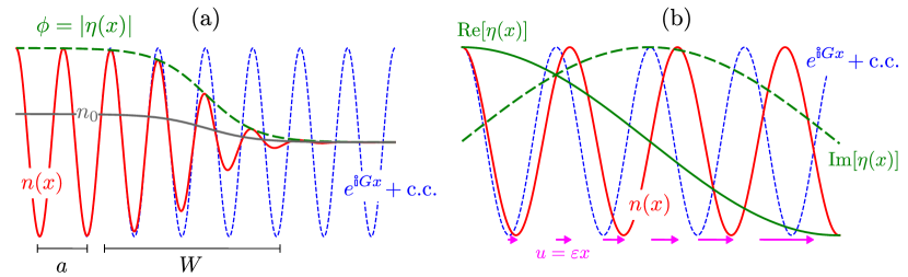
Figure 1: (a) Sample (1D) liquid/solid interface, where $a$ is the atomic spacing and $W$ is the width of the interface. (b) Sample (1D) deformed lattice by displacement $u=\varepsilon x$.

2.2 Derivation

There are various methods for deriving the amplitude expansion from the original PFC model. Essentially, it requires a separation of length scales by assuming that the complex amplitudes vary on length scales much larger than the atomic spacing. In general this is the same assumption of all phase field models which require that interfaces or domain walls make a smooth transition from one phase to another. This is illustrated in Fig. 1 for a one dimensional liquid/solid interface for a system of atomic spacing $a$ and interface width $W$. The “phase field limit” is such that $a/W\ll 1$. For instance, for a two-dimensional triangular lattice it can be shown [45] that in the limit that $n_{\rm o}=0$ and the complex amplitudes are real and identical (i.e., $\eta_{\texttt{h}\texttt{k}\texttt{l}}=\phi$, for all hkl), they are described by traveling wave solutions (with velocity $V$) of the form,

$$\phi=A\bigg{[}1-\tanh\bigg{(}\frac{x-Vt}{W}\bigg{)}\bigg{]},$$ (4)

where $W$ is the width of the liquid/solid front which can be written [45] as

$$W=\frac{W^{m}}{1+\sqrt{1-(8/9)\Delta\texttt{B}^{0}/\Delta\texttt{B}^{0}_{\rm ls}}},$$ (5)

where $\Delta\texttt{B}^{0}_{\rm ls}=8\texttt{t}^{2}/135\texttt{v}$ is the value of $\Delta\texttt{B}^{0}$ at liquid/solid coexistence and $W^{m}$ is the maximum value of $W$ and is given by

$$W^{m}=2q_{0}\sqrt{30\texttt{v}\texttt{B}^{x}}/\texttt{t}.$$ (6)

For $\Delta\texttt{B}^{0}>9/8\Delta\texttt{B}^{0}_{\rm ls}$ no traveling wave solution exists as the solid is linearly unstable. Thus the phase field limit occurs when $\texttt{B}^{x}\rightarrow\infty$ and as such $1/\texttt{B}^{x}$ can be used as a small parameter in a multi-scale calculation. In light of this, it is convenient to make the following rescaling, $\epsilon=-\Delta\texttt{B}^{0}/\texttt{B}^{x}$, $\bar{n}=n(\texttt{v}/\texttt{B}^{x})^{1/2}$, $\bar{F}=F\texttt{v}/(\texttt{B}^{x})^{2}$, so that Eq. (1) can be written

$$\bar{F}=\int\text{d}\mathbf{r}\left[-\frac{\epsilon}{2}\bar{n}^{2}+\frac{1}{2}\bar{n}(q_{0}^{2}+\nabla^{2})^{2}\bar{n}-\frac{\tau}{3}\bar{n}^{3}+\frac{1}{4}\bar{n}^{4}\right],$$ (7)

where $\tau=\texttt{t}/\sqrt{\texttt{v}\texttt{B}^{x}}$. Now the limit $\texttt{B}^{x}\rightarrow\infty$ corresponds to $\epsilon\rightarrow 0$.

Goldenfeld and co-workers [22, 23] report that to obtain rotationally invariant equations using multiple-scales analysis requires going to sixth order perturbations, which is an extremely tedious task, as to lowest order the resulting equations are not rotationally invariant. However, they have shown that this analysis gives the same result using a simpler renormalization group calculation. Other works addressed refinement and assessment of the general renormalization group approach [46, 47].

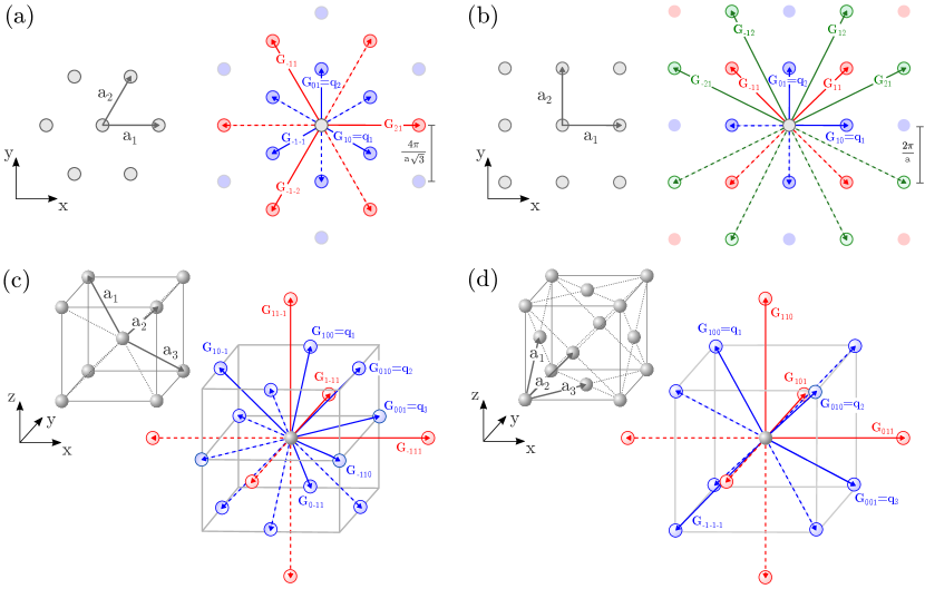
Figure 2: Crystal structures (grey) and corresponding shortest reciprocal lattice vectors (colored): (a) triangular, (b) square, (c) body-centered cubic, (d) face-centered cubic. Arrows represent the reciprocal space vectors entering Eq. (3) in the one- (blue) and two- (blue and red) mode approximations. For the square lattice the additional reciprocal-space vectors considered in a three-mode approximation involving non-parallel vectors only are also shown (green). Solid arrows indicate an explicit choice of vectors entering Eq. (17) (as exploited from Sec. 2.3.2 on).

To grasp the essence of the calculations without using these more rigorous methods, Athreya et al[23] developed a method that was coined “quick and dirty” that essentially obtains the same result in the $W\rightarrow\infty$ limit. The basic idea is to assume that the amplitudes are constant on atomic length scales, i.e.,

$$\int_{\rm u.c.}d\mathbf{r}\,f(\eta_{\texttt{h}\texttt{k}\texttt{l}})\rme^{{\mathbb{i}}\mathbf{q}\cdot\mathbf{r}}\approx f(\eta_{\texttt{h}\texttt{k}\texttt{l}})\int_{\rm u.c.}d\mathbf{r}\,\rme^{{\mathbb{i}}\mathbf{q}\cdot\mathbf{r}},$$ (8)

where $\int_{\rm u.c.}$ is an integration over a unit cell and $\mathbf{q}$ is a sum over various $\mathbf{G}_{\texttt{h}\texttt{k}\texttt{l}}$. Since $\mathbf{q}$ is periodic in the unit cell, Eq. (8) is zero unless $\mathbf{q}=0$. This is a considerable simplification that reduces the number of terms that enter the free energy. For example, consider a term

$$\begin{split}\int d\mathbf{r}\,n^{2}=\int d\mathbf{r}\bigg{[}n_{\rm o}^{2}+2n_{\rm o}\bigg{(}\sum_{\texttt{h}\texttt{k}\texttt{l}}\eta_{\texttt{h}\texttt{k}\texttt{l}}\rme^{{\mathbb{i}}\mathbf{G}_{\texttt{h}\texttt{k}\texttt{l}}\cdot\mathbf{r}}\bigg{)}+\bigg{(}\sum_{\texttt{h}\texttt{k}\texttt{l}}\eta_{\texttt{h}\texttt{k}\texttt{l}}\rme^{{\mathbb{i}}\mathbf{G}_{\texttt{h}\texttt{k}\texttt{l}}\cdot\mathbf{r}}\bigg{)}\bigg{(}\sum_{\texttt{h}^{\prime}\texttt{k}^{\prime}\texttt{l}^{\prime}}\eta_{\texttt{h}^{\prime}\texttt{k}^{\prime}\texttt{l}^{\prime}}\rme^{{\mathbb{i}}\mathbf{G}_{\texttt{h}^{\prime}\texttt{k}^{\prime}\texttt{l}^{\prime}}\cdot\mathbf{r}}\bigg{)}\bigg{]}.\end{split}$$ (9)

Only the first and last term for $\texttt{h}\texttt{k}\texttt{l}=-(\texttt{h}^{\prime}\texttt{k}^{\prime}\texttt{l}^{\prime})$ give non-zero contributions using approximation Eq. (8), since they do not contain terms multiplied by a periodic function. Thus, in this approximation, Eq. (9) reduces to

$$\int d\mathbf{r}\,n^{2}\approx\int d\mathbf{r}\bigg{[}n_{\rm o}^{2}+\sum_{\texttt{h}\texttt{k}\texttt{l}}|\eta_{\texttt{h}\texttt{k}\texttt{l}}|^{2}\bigg{]}.$$ (10)

As discussed in the next section, contributions that arise from higher order polynomial terms will depend on the specific crystal symmetry under consideration. Terms containing the $\nabla^{2}$ operator are treated similarly noting that, assuming constant or slowly varying $n_{\rm o}$,

$$\nabla^{2}n=\sum_{\texttt{h}\texttt{k}\texttt{l}}\rme^{{\mathbb{i}}\mathbf{G}_{\texttt{h}\texttt{k}\texttt{l}}\cdot\mathbf{r}}\underbrace{(\nabla^{2}+2{\mathbb{i}}\mathbf{G}_{\texttt{h}\texttt{k}\texttt{l}}\cdot\vec{\nabla}-|\mathbf{G}_{\texttt{h}\texttt{k}\texttt{l}}|^{2})}_{\mathcal{L}_{\texttt{h}\texttt{k}\texttt{l}}}\eta_{\texttt{h}\texttt{k}\texttt{l}}.$$ (11)

Thus the Laplacian operator transforms as $\nabla^{2}\rightarrow\mathcal{L}_{\texttt{h}\texttt{k}\texttt{l}}$. While the effective operator on the right hand side of Eq. (11) appears to be anisotropic (due to the specific direction of the $\mathbf{G}_{\texttt{h}\texttt{k}\texttt{l}}$’s), it can be shown that the free energy is independent of the orientation of the pattern formed in $n$ [48]. With these steps an energy functional which depends on amplitudes, $F_{\eta}$, can be derived (see also Sec. 2.3).

The dynamics of $\eta_{\texttt{h}\texttt{k}\texttt{l}}$ approximating (2) can be obtained by multiplying Eq. (2) by $\rme^{-{\mathbb{i}}\mathbf{G}_{\texttt{h}\texttt{k}\texttt{l}}\cdot\mathbf{r}}$ and integrating over a unit cell, i.e.,

$$\int_{\rm u.c.}\frac{d\mathbf{r}}{V}\,\rme^{-{\mathbb{i}}\mathbf{G}_{\texttt{h}\texttt{k}\texttt{l}}\cdot\mathbf{r}}\,\frac{\partial n}{\partial t}\approx\frac{\partial\eta_{\texttt{h}\texttt{k}\texttt{l}}}{\partial t},$$ (12)

where $V$ is the volume of a unit cell, which may be written as

$$\frac{\partial\eta_{\texttt{h}\texttt{k}\texttt{l}}}{\partial t}=\mathcal{L}_{\texttt{h}\texttt{k}\texttt{l}}\frac{\delta F_{\eta}}{\delta\eta_{\texttt{h}\texttt{k}\texttt{l}}^{*}}=(\nabla^{2}+{\mathbb{i}}\mathbf{G}_{\texttt{h}\texttt{k}\texttt{l}}\cdot\nabla-|\mathbf{G}_{\texttt{h}\texttt{k}\texttt{l}}|^{2})\frac{\delta F_{\eta}}{\delta\eta_{\texttt{h}\texttt{k}\texttt{l}}^{*}}\approx-|\mathbf{G}_{\texttt{h}\texttt{k}\texttt{l}}|^{2}\frac{\delta F_{\eta}}{\delta\eta_{\texttt{h}\texttt{k}\texttt{l}}^{*}},$$ (13)

where the long-wavelength limit has been used in the last approximation. It is interesting to note that the equation of motion for the amplitudes are non-conserved, implying that an initial liquid (crystal) can completely transform in a crystal (liquid) locally.

Nevertheless the density is a conserved quantity in a closed system and it is often important in liquid solid transitions since in liquid/solid coexistence the liquid and solid have different densities. In addition, the process of dislocation climb involves the mass (or vacancy) diffusion. In the original derivation of the APFC [22, 23] the average density was assumed to be constant. The first inclusion of a spatially dependent density was reported by Yeon et al[49]. In this work $n_{\rm o}$ was assumed to vary on the same length scales as the complex amplitudes and Eq. (3) should read

$$n({\bf r},t)=n_{\rm o}({\bf r},t)+\sum_{\texttt{h}\texttt{k}\texttt{l}}\eta_{\texttt{h}\texttt{k}\texttt{l}}({\bf r},t)\rme^{{\mathbb{i}}\mathbf{G}_{\texttt{h}\texttt{k}\texttt{l}}\cdot{\bf r}}.$$ (14)

Unfortunately, using the so-called “quick and dirty” method leads to an equation of motion for $n_{\rm o}$ (and free energy) which contains terms like $(1+\nabla^{2})^{2}n$ and then implies that crystal state can be obtained from constant amplitudes or by a periodically varying $n_{\rm o}$ (which of course violates the assumption the $n_{\rm o}$ varies on the same length scales as the amplitudes). To overcome this difficulty several simpler models were proposed, which were shown to incorporate interfacial energy associated with the density difference at liquid/solid front as well as the well known Gibbs-Thomson effect [49]. The model can be written

$$\begin{split}{\cal F}=&\int{\rm d}\mathbf{r}\bigg{[}\frac{\Delta\texttt{B}^{0}}{2}n_{\rm o}^{2}-\frac{\texttt{t}}{3}n_{\rm o}^{3}+\frac{\texttt{v}}{4}n_{\rm o}^{4}+\frac{1}{2}\left(\Delta\texttt{B}^{0}-2\texttt{t}n_{\rm o}+3\texttt{v}n_{\rm o}^{2}\right)\bigg{(}\sum_{\texttt{h}\texttt{k}\texttt{l}}\eta_{\texttt{h}\texttt{k}\texttt{l}}\rme^{{\mathbb{i}}\mathbf{G}_{\texttt{h}\texttt{k}\texttt{l}}\cdot\mathbf{r}}\bigg{)}^{2}\\ &-\frac{1}{3}\left(\texttt{t}-3n_{\rm o}\right)\bigg{(}\sum_{\texttt{h}\texttt{k}\texttt{l}}\eta_{\texttt{h}\texttt{k}\texttt{l}}\rme^{{\mathbb{i}}\mathbf{G}_{\texttt{h}\texttt{k}\texttt{l}}\cdot\mathbf{r}}\bigg{)}^{3}+\frac{\texttt{v}}{4}\bigg{(}\sum_{\texttt{h}\texttt{k}\texttt{l}}\eta_{\texttt{h}\texttt{k}\texttt{l}}\rme^{{\mathbb{i}}\mathbf{G}_{\texttt{h}\texttt{k}\texttt{l}}\cdot\mathbf{r}}\bigg{)}^{4}+\frac{\texttt{B}^{x}}{2}\sum_{\texttt{h}\texttt{k}\texttt{l}}(|\mathcal{L}_{\texttt{h}\texttt{k}\texttt{l}}+q_{0}^{2})\eta_{\texttt{h}\texttt{k}\texttt{l}}|^{2}\bigg{]},\end{split}$$ (15)

with dynamics

$$\frac{\partial\eta_{\texttt{h}\texttt{k}\texttt{l}}}{\partial t}=-|\mathbf{G}_{\texttt{h}\texttt{k}\texttt{l}}|^{2}\frac{\delta{\cal F}}{\delta\eta_{\texttt{h}\texttt{k}\texttt{l}}^{*}},\ \ \ \ \ \frac{\partial n_{\rm o}}{\partial t}=\nabla^{2}\frac{\delta{\cal F}}{\delta n_{\rm o}}.$$ (16)

The specific terms that emerge when averaged over a unit cell are discussed in the following section. This approach is also discussed in Huang et al[29]. If the amplitudes are assumed to be real (which eliminates the possibility of elastic and plastic phenomena) this reduces to Model C in the Hohenberg/Halperin [50] classification scheme that can be used to study phenomena such as directional solidification [51] or eutectic solidification [52, 53]. Heinonen et al[54] use a similar free energy functional, but also incorporate momentum through the Navier Stokes equation and add the corresponding convective term to the dynamics of $\eta_{\texttt{h}\texttt{k}\texttt{l}}$ and $n_{\rm o}$. This has the advantage of including faster relaxation of elastic fields as discussed in Sec. 5.2.

2.3 Formulas for amplitude equations

Let’s consider the free energy Eq. (1) with constant average density $n_{\rm o}$ and for the sake of simplicity the generic parameters $A=\texttt{B}^{x}$, $B=\Delta\texttt{B}^{0}-2\texttt{t}n_{\rm o}+3\texttt{v}n_{\rm o}^{2}$, $C=-(\texttt{t}+3n_{\rm o})$, $D=\texttt{v}$, $E=\Delta\texttt{B}^{0}n_{\rm o}^{2}/2-\texttt{t}n_{\rm o}^{3}/3+\texttt{v}n_{\rm o}^{4}/4$. The amplitude expansion is based on the approximation of $n$ as from Eq. (3) with a finite set of $M$ vectors $\mathbf{G}_{\texttt{h}\texttt{k}\texttt{l}}$, reproducing a specific crystal symmetry. This equation, exploiting that $\eta_{-(\texttt{h}\texttt{k}\texttt{l})}=\eta_{\texttt{h}\texttt{k}\texttt{l}}^{*}$, is here rewritten as

$$n=n_{\rm o}+\sum_{m=1}^{M}\eta_{m}\rme^{{\mathbb{i}}\mathbf{G}_{m}\cdot\mathbf{r}}+\text{c.c.}$$ (17)

where for simplicity $\mathbf{G}_{\texttt{h}\texttt{k}\texttt{l}}$ is given a single subscript $m$ and c.c. is the complex conjugate, highlighting the minimal set of amplitudes to be considered to approximate $n$. The free energy and the evolution law for the amplitudes can be obtained by exploiting the coarse-graining procedure introduced in Sec. 2.2, i.e. by integration over the unit cell of the phase-field crystal energy density (1), with $n$ expressed through its amplitude expansion, Eq. (17) [55, 56, 57, 48, 58].

To provide a general form of the free energy, consider separately the different powers of $n$ entering Eq. (1), namely $n^{k}(\{\eta_{m}\},\{\eta_{m}^{*}\})\rightarrow\zeta_{k}$. After averaging over a unit cell the following results emerge,

$$\begin{split}\zeta_{2}\ =\ 2\ &{\textstyle\sum^{M}_{m}}\ |\eta_{m}|^{2}=\Phi,\\ \zeta_{3}\ =\ \bigg{[}3&{\textstyle\sum_{n>m}^{M}}\ \big{\{}\mathcal{K}_{2m+n}\eta_{m}^{2}\eta_{n}+\mathcal{K}_{m+2n}\eta_{m}\eta_{n}^{2}+\mathcal{K}_{-2m+n}{\eta_{m}^{*}}^{2}\eta_{n}+\mathcal{K}_{-m+2n}\eta_{m}^{*}\eta_{n}^{2}\big{\}}\\ +6&{\textstyle\sum^{M}_{o>n>m}}\big{\{}\mathcal{K}_{m+n+o}\eta_{m}\eta_{n}\eta_{o}+\mathcal{K}_{-m+n+o}\eta_{m}^{*}\eta_{n}\eta_{o}+\mathcal{K}_{m-n+o}\eta_{m}\eta_{n}^{*}\eta_{o}\\ &\ \qquad\quad+\mathcal{K}_{m+n-o}\eta_{m}\eta_{n}\eta_{o}^{*}\big{\}}+\text{c.c.}\bigg{]},\\ \zeta_{4}\ =\ 6\ &{\textstyle\sum^{M}_{m}}\ |\eta_{m}|^{4}+24{\textstyle\sum^{M}_{n>m}}|\eta_{m}|^{2}|\eta_{n}|^{2}\\ +\bigg{[}4&{\textstyle\sum_{n>m}^{M}}\big{\{}\mathcal{K}_{3m+n}\eta_{m}^{3}\eta_{n}+\mathcal{K}_{-3m+n}{\eta_{m}^{*}}^{3}\eta_{n}+\mathcal{K}_{-m+3n}\eta_{m}^{*}\eta_{n}^{3}+\mathcal{K}_{m+3n}\eta_{m}\eta_{n}^{3}\big{\}}\\ +12&{\textstyle\sum^{M}_{o>n>m}}\big{\{}\mathcal{K}_{2m+n+o}\eta_{m}^{2}\eta_{n}\eta_{o}+\mathcal{K}_{m+2n+o}\eta_{m}\eta_{n}^{2}\eta_{o}+\mathcal{K}_{m+n+2o}\eta_{m}\eta_{n}\eta_{o}^{2}\\ &\ \qquad\quad+\mathcal{K}_{-2m+n+o}{\eta_{m}^{*}}^{2}\eta_{n}\eta_{o}+\mathcal{K}_{-m+2n+o}\eta_{m}^{*}\eta_{n}^{2}\eta_{o}+\mathcal{K}_{-m+n+2o}\eta_{m}^{*}\eta_{n}\eta_{o}^{2}\\ &\ \qquad\quad+\mathcal{K}_{2m-n+o}\eta_{m}^{2}\eta_{n}^{*}\eta_{o}+\mathcal{K}_{m-2n+o}\eta_{m}{\eta_{n}^{*}}^{2}\eta_{o}\mathcal{K}_{m-n+2o}\eta_{m}\eta_{n}^{*}\eta_{o}^{2}\\ &\ \qquad\quad+\mathcal{K}_{2m+n-o}\eta_{m}^{2}\eta_{n}\eta_{o}^{*}+\mathcal{K}_{m+2n-o}\eta_{m}\eta_{n}^{2}\eta_{o}^{*}+\mathcal{K}_{m+n-2o}\eta_{m}\eta_{n}{\eta_{o}^{*}}^{2}\big{\}}\\ +24&{\textstyle\sum^{M}_{p>o>n>m}}\big{\{}\mathcal{K}_{-m+n+o+p}\eta_{m}^{*}\eta_{n}\eta_{o}\eta_{p}+\mathcal{K}_{m-n+o+p}\eta_{m}\eta_{n}^{*}\eta_{o}\eta_{p}\\ &\ \qquad\qquad+\mathcal{K}_{m+n-o+p}\eta_{m}\eta_{n}\eta_{o}^{*}\eta_{p}+\mathcal{K}_{m+n+o-p}\eta_{m}\eta_{n}\eta_{o}\eta_{p}^{*}\\ &\ \qquad\qquad+\mathcal{K}_{-m-n+o+p}\eta_{m}^{*}\eta_{n}^{*}\eta_{o}\eta_{p}+\mathcal{K}_{-m+n-o+p}\eta_{m}^{*}\eta_{n}\eta_{o}^{*}\eta_{p}\\ &\ \qquad\qquad+\mathcal{K}_{-m+n+o-p}\eta_{m}^{*}\eta_{n}\eta_{o}\eta_{p}^{*}+\mathcal{K}_{m+n+o+p}\eta_{m}\eta_{n}\eta_{o}\eta_{p}\big{\}}+\text{c.c.}\bigg{]},\end{split}$$ (18)

with

$$\begin{split}\mathcal{K}_{im+jn+ko+lp}&=\begin{cases}1&\text{if}\ \ |i\mathbf{G}_{m}+j\mathbf{G}_{n}+k\mathbf{G}_{o}+l\mathbf{G}_{p}|=0\\ 0&\text{if}\ \ |i\mathbf{G}_{m}+j\mathbf{G}_{n}+k\mathbf{G}_{o}+l\mathbf{G}_{p}|\neq 0\end{cases},\end{split}$$ (19)

and neglecting terms including a factor $\mathcal{K}_{im+in}$ with $i=\pm 1,\pm 2$ which would appear in $\zeta_{2}$ and $\zeta_{4}$ as $\mathbf{G}_{m}$ with the same lengths are never parallel (or antiparallel), so $\mathcal{K}_{im+in}=0$. Notice that terms as in the first sum in $\zeta_{3}$ or the third sum of $\zeta_{4}$ contributes if considering modes with two or three times the length of others, respectively (e.g. $\mathbf{G}_{10}$ and $\mathbf{G}_{20}$ in Fig. 2(b)).

For a one-mode approximation of $n$ through Eq. (17), i.e. by considering the shortest $\mathbf{G}_{m}$, and transformation (11), the excess term becomes

$$\begin{split}\int_{\rm u.c.}d{\bf r}\ n(1+\nabla^{2})^{2}n=\sum^{M}_{m}2|(1+\mathcal{L}_{m})\eta_{m}|^{2}\stackrel{{\scriptstyle|\mathbf{G}_{m}|=1}}{{=}}\sum^{M}_{m}2|\mathcal{G}_{m}\eta_{m}|^{2},\end{split}$$ (20)

with $\mathcal{G}_{m}=\nabla^{2}+2{\mathbb{i}}\mathbf{G}_{m}\cdot\nabla$ and $\mathcal{L}_{m}=\mathcal{G}_{m}-|\mathbf{G}_{m}|^{2}$. In the one mode approximation, the length scales can always be re-parametrized such that $|\mathbf{G}_{m}|=1$.

Interestingly the term $\zeta_{2}=\Phi$ does not depend on the lattice symmetry, while $\zeta_{4}$ can be written $\zeta_{4}=6\sum_{m}^{M}|\eta_{m}|^{4}+24\sum^{M}_{n>m}|\eta_{m}|^{2}|\eta_{n}|^{2}+\zeta_{4}^{\rm s}=3\Phi^{2}-6\sum_{m}^{M}|\eta_{m}|^{4}+\zeta_{4}^{\rm s}$, where $\zeta_{4}^{\rm s}$ depends on lattice symmetry. Therefore, the free energy as function of amplitudes may be written

$$\begin{split}F_{\eta}&=\int_{\Omega}\text{d}\mathbf{r}\bigg{[}\frac{A}{2}\sum_{m}^{M}2|\mathcal{G}_{m}\eta_{m}|^{2}+\frac{B}{2}\zeta_{2}+\frac{C}{3}\zeta_{3}+\frac{D}{4}\zeta_{4}+E\bigg{]}\\ &=\int_{\Omega}\text{d}\mathbf{r}\bigg{[}\frac{B}{2}\Phi+\frac{3D}{4}\Phi^{2}+\sum_{m}^{M}\left(A|\mathcal{G}_{m}\eta_{m}|^{2}-\frac{3D}{2}|\eta_{m}|^{4}\right)+f^{\rm s}(\{\eta_{m}\},\{\eta_{m}^{*}\})+E\bigg{]},\end{split}$$ (21)

with $f^{\rm s}(\{\eta_{m}\},\{\eta_{m}^{*}\})=\frac{C}{3}\zeta_{3}+\frac{D}{4}\zeta_{4}^{\rm s}$.

The dynamics of the amplitudes, based on the PFC formulation in Eq. (2) and according to transformation (12) are given by

$$\frac{\partial\eta_{m}}{\partial t}=\mathcal{L}_{m}\frac{\delta F_{\eta}}{\delta\eta_{m}^{*}}\approx-|\mathbf{G}_{m}|^{2}\bigg{[}A\mathcal{G}_{m}^{2}\eta_{m}+B\eta_{m}+3D(\Phi-|\eta_{m}|^{2})\eta_{m}+\underbrace{\frac{C}{3}\frac{\partial\zeta_{3}}{\partial\eta_{m}^{*}}+\frac{D}{4}\frac{\partial\zeta_{4}^{\rm s}}{\partial\eta_{m}^{*}}}_{\partial f^{\rm s}/\partial\eta_{m}^{*}}\bigg{]},$$ (22)

where $\mathcal{L}_{m}\approx-|\mathbf{G}_{m}|^{2}$ as in Eq. (13), and, from Eq. (18),

$$\begin{split}\frac{1}{3}\frac{\partial\zeta_{3}}{\partial\eta_{m}^{*}}\ =\ &{\textstyle\sum_{n\neq m}^{M}}\big{\{}2\mathcal{K}_{-2m-n}\eta_{m}^{*}\eta_{n}^{*}+2\mathcal{K}_{-2m+n}\eta_{m}^{*}\eta_{n}+\mathcal{K}_{-m-2n}{\eta_{n}^{*}}^{2}+\mathcal{K}_{-m+2n}\eta_{n}^{2}\big{\}}\\ +2&{\textstyle\sum^{M}_{o>n\neq m}}\big{\{}\mathcal{K}_{-m-n-o}\eta_{n}^{*}\eta_{o}^{*}+\mathcal{K}_{-m+n+o}\eta_{n}\eta_{o}+\mathcal{K}_{-m+n-o}\eta_{n}\eta_{o}^{*}+\mathcal{K}_{-m-n+o}\eta_{n}^{*}\eta_{o}\big{\}},\\ \frac{1}{4}\frac{\partial\zeta_{4}^{\rm s}}{\partial\eta_{m}^{*}}\ =\ &{\textstyle\sum_{n\neq m}^{M}}\big{\{}3\mathcal{K}_{-3m-n}{\eta_{m}^{*}}^{2}\eta_{n}^{*}+3\mathcal{K}_{-3m+n}{\eta_{m}^{*}}^{2}\eta_{n}+\mathcal{K}_{-m+3n}\eta_{n}^{3}+\mathcal{K}_{-m-3n}{\eta_{n}^{*}}^{3}\big{\}}\\ +3&{\textstyle\sum^{M}_{o>n\neq m}}\big{\{}2\mathcal{K}_{-2m-n-o}\eta_{m}^{*}\eta_{n}^{*}\eta_{o}^{*}+\mathcal{K}_{-m-2n-o}{\eta_{n}^{*}}^{2}\eta_{o}^{*}+\mathcal{K}_{-m-n-2o}\eta_{n}^{*}{\eta_{o}^{*}}^{2}\\ &\qquad\qquad+2\mathcal{K}_{-2m+n+o}\eta_{m}^{*}\eta_{n}\eta_{o}+\mathcal{K}_{-m+2n+o}\eta_{n}^{2}\eta_{o}+\mathcal{K}_{-m+n+2o}\eta_{n}\eta_{o}^{2}\\ &\qquad\qquad+2\mathcal{K}_{-2m+n-o}\eta_{m}^{*}\eta_{n}\eta_{o}^{*}+\mathcal{K}_{-m+2n-o}\eta_{n}^{2}\eta_{o}^{*}+\mathcal{K}_{-m+n-2o}\eta_{n}{\eta_{o}^{*}}^{2}\\ &\qquad\qquad+2\mathcal{K}_{-2m-n+o}\eta_{m}^{*}\eta_{n}^{*}\eta_{o}+\mathcal{K}_{-m-2n+o}{\eta_{n}^{*}}^{2}\eta_{o}+\mathcal{K}_{-m-n+2o}\eta_{n}^{*}\eta_{o}^{2}\big{\}}\\ +6&{\textstyle\sum^{M}_{p>o>n\neq m}}\big{\{}\mathcal{K}_{-m+n+o+p}\eta_{n}\eta_{o}\eta_{p}+\mathcal{K}_{-m+n-o-p}\eta_{n}\eta_{o}^{*}\eta_{p}^{*}+\mathcal{K}_{-m-n+o-p}\eta_{n}^{*}\eta_{o}\eta_{p}^{*}\\ &\qquad\qquad+\mathcal{K}_{-m-n-o+p}\eta_{n}^{*}\eta_{o}^{*}\eta_{p}+\mathcal{K}_{-m-n+o+p}\eta_{n}^{*}\eta_{o}\eta_{p}+\mathcal{K}_{-m+n-o+p}\eta_{n}\eta_{o}^{*}\eta_{p}\\ &\qquad\qquad+\mathcal{K}_{-m+n+o-p}\eta_{n}\eta_{o}\eta_{p}^{*}+\mathcal{K}_{-m-n-o-p}\eta_{n}^{*}\eta_{o}^{*}\eta_{p}^{*}\big{\}},\end{split}$$ (23)

2.3.1 Multi-mode approximations.

To model some crystal lattices, more than one mode is required in Eq. (17), i.e. more length scales are set through the choice of the reciprocal space vectors. In this case, $\zeta_{m}$ reads as reported above, but the excess term takes different forms. However, it may be reduced to Eq. (20) through approximation [6, 13]. For two lengths, $R_{1}=2\pi/k^{\rm eq}_{1}$ and $R_{2}=2\pi/k^{\rm eq}_{2}$, corresponding to different lengths in the reciprocal space $k^{\rm eq}_{1}=1$ and $k^{\rm eq}_{2}=\alpha k^{\rm eq}_{1}$, with $\alpha\neq 1=k^{\rm eq}_{2}/k^{\rm eq}_{1}=R_{1}/R_{2}$, the term including the differential operator in the dynamic would read [6]

$$(1+R_{1}^{2}\nabla^{2})^{2}(1+R_{2}^{2}\nabla^{2})^{2}n\rightarrow\sum^{M}_{m}\alpha^{-4}(1+\mathcal{L}_{m})^{2}(\alpha^{2}+\mathcal{L}_{m})^{2}\eta_{m}=\sum^{M}_{m}\mathcal{D}_{m}\eta_{m},$$ (24)

with

$$\mathcal{D}_{m}=\begin{cases}\alpha^{-4}(\mathcal{G}_{m})^{2}(\alpha^{2}-1+\mathcal{G}_{m})^{2}=\frac{(\alpha^{2}-1)^{2}}{\alpha^{4}}(\mathcal{G}_{m})^{2}\big{(}1+\frac{\mathcal{G}_{m}}{\alpha^{2}-1}\big{)}^{2}&\text{if}\ |\mathbf{G}_{m}|=k^{\rm eq}_{1}=1\\ \alpha^{-4}(1-\alpha^{2}+\mathcal{G}_{m})^{2}(\mathcal{G}_{m})^{2}=\frac{(1-\alpha^{2})^{2}}{\alpha^{4}}(\mathcal{G}_{m})^{2}\big{(}1-\frac{\mathcal{G}_{m}}{\alpha^{2}-1}\big{)}^{2}&\text{if}\ |\mathbf{G}_{m}|=k^{\rm eq}_{2}=\alpha\end{cases}$$ (25)

and lengths have been scaled such that $\mathbf{x}\rightarrow\mathbf{x}/R_{1}$. If $2|\mathcal{G}_{m}\eta_{m}|\ll|(\alpha^{2}-1)\eta_{m}|$,

$$\mathcal{D}_{m}\eta_{m}\approx\frac{(\alpha^{2}-1)^{2}}{\alpha^{4}}\mathcal{G}_{m}^{2}\eta_{m}.$$ (26)

Therefore, the coefficient $A$ can be rescaled by a factor $\alpha^{4}/(\alpha^{2}-1)^{2}$ and the same energy term as for the one mode approximation can be used. This result may be generalized for a lattice having $N_{\ell}$ different length scales $R_{\ell}=2\pi/k^{\rm eq}_{\ell}$ and $k^{\rm eq}_{\ell}/k^{\rm eq}_{1}=\alpha_{\ell}$ (noting $k_{1}^{\rm eq}=1$). Eq. (24) would read

$$\prod_{\ell}^{N_{\ell}}(1+R_{\ell}^{2}\nabla^{2})^{2}n\rightarrow\sum^{M}_{m}\bigg{[}\prod_{\ell}^{N_{\ell}}(1+\alpha_{\ell}^{-2}\mathcal{L}_{m})^{2}\bigg{]}\eta_{m}=\sum^{M}_{m}\mathcal{M}_{m}\eta_{m}.$$ (27)

If, $\forall\ell$, $2|\mathcal{G}_{m}\eta_{m}|\ll|(\alpha^{2}_{\ell}-|\mathbf{G}_{m}|^{2})|\eta_{m}$, one may write

$$\mathcal{M}_{m}\eta_{m}\approx\left[|\mathbf{G}_{m}|^{-4}\prod_{\begin{subarray}{c}\ell\\ \alpha_{\ell}\neq|\mathbf{G}_{m}|\end{subarray}}^{N_{\ell}}\bigg{(}\frac{\alpha_{\ell}^{2}-|\mathbf{G}_{m}|^{2}}{\alpha_{\ell}^{2}}\bigg{)}^{2}\right]\mathcal{G}_{m}^{2}\eta_{m}=\Gamma_{m}\mathcal{G}_{m}^{2}\eta_{m},$$ (28)

that for $N_{l}=2$, $\alpha_{1}=1$ and $\alpha_{2}=\alpha$ reduces to Eq. (26). Then, under this approximation, $\sum^{M}_{m}\mathcal{M}_{m}\eta_{m}=\sum^{M}_{m}\Gamma_{m}\mathcal{G}_{m}^{2}\eta_{m}$. Notice that in the presence of more than two modes, the coefficient of $\mathcal{G}_{m}^{2}$ cannot be taken outside the sum so it cannot be included in the coefficient $A$ through rescaling as in Eq. (26).

2.3.2 Results for specific lattice symmetries.

Implementations of the APFC equations may be performed in a general fashion by considering Eqs. (18) and (23). This delivers a general framework suitable for changes in lattice symmetries and the number of modes used (eventually also different symmetries at once, see also Sec. 6.4). However, the specific equations corresponding to given lattice symmetries through the choice of reciprocal lattice vectors may be useful for analytic calculations and ad-hoc implementations. In the following, $f^{\rm s}\equiv f^{\rm s}({\{\eta_{m}\},\{\eta_{m}^{*}\}})$ are reported for selected crystal symmetries used in literature, with the length of shortest reciprocal space vectors normalized to $1$ (see, e.g., [6, 59, 60, 61] and Fig. 2).

Triangular (TRI) symmetry (2D), one-mode approximation, $N=3$:

$$\mathbf{G}_{1}^{\rm TRI}=\begin{bmatrix}-\sqrt{3}/2\\ -1/2\\ \end{bmatrix},\quad\mathbf{G}_{2}^{\rm TRI}=\begin{bmatrix}0\\ 1\\ \end{bmatrix},\quad\mathbf{G}_{3}^{\rm TRI}=\begin{bmatrix}\sqrt{3}/2\\ -1/2\\ \end{bmatrix},$$

$$f^{\rm tri,1}=2C(\eta_{1}\eta_{2}\eta_{3}+\eta_{1}^{*}\eta_{2}^{*}\eta_{3}^{*}).$$ (29)

Triangular (TRI) symmetry (2D), two-mode approximation, $N=6$:

$$\mathbf{G}_{1}^{\rm TRI},\quad\mathbf{G}_{2}^{\rm TRI},\quad\mathbf{G}_{3}^{\rm TRI},\quad\mathbf{G}_{4}^{\rm TRI}=\mathbf{G}_{1}^{\rm TRI}-\mathbf{G}_{2}^{\rm TRI},$$

$$\quad\mathbf{G}_{5}^{\rm TRI}=\mathbf{G}_{2}^{\rm TRI}-\mathbf{G}_{3}^{\rm TRI},\quad\mathbf{G}_{6}^{\rm TRI}=\mathbf{G}_{3}^{\rm TRI}-\mathbf{G}_{1}^{\rm TRI},$$

$$\begin{split}f^{\rm tri,2}=&2C(\eta_{1}\eta_{2}\eta_{3}+\eta_{1}^{*}\eta_{2}\eta_{4}+\eta_{1}\eta_{3}^{*}\eta_{6}+\eta_{2}^{*}\eta_{3}\eta_{5}+\eta_{4}\eta_{5}\eta_{6})\\ &+3D(\eta_{1}\eta_{2}^{2}\eta_{5}^{*}+\eta_{1}^{2}\eta_{2}\eta_{6}+\eta_{1}^{2}\eta_{3}\eta_{4}^{*}+\eta_{1}\eta_{3}^{2}\eta_{5}+\eta_{2}^{2}\eta_{3}\eta_{4}+\eta_{2}\eta_{3}^{2}\eta_{6}^{*})\\ &+6D(\eta_{1}\eta_{2}^{*}\eta_{5}\eta_{6}+\eta_{1}^{*}\eta_{3}\eta_{4}\eta_{5}+\eta_{2}\eta_{3}^{*}\eta_{4}\eta_{6})+\text{c.c.}\end{split}$$ (30)

Square (SQ) symmetry (2D), two-mode approximation, $N=4$:

$$\mathbf{G}_{1}^{\rm SQ}=\begin{bmatrix}1\\ 0\\ \end{bmatrix},\quad\mathbf{G}_{2}^{\rm SQ}=\begin{bmatrix}0\\ 1\\ \end{bmatrix},\quad\mathbf{G}_{3}^{\rm SQ}=\begin{bmatrix}1\\ 1\\ \end{bmatrix},\quad\mathbf{G}_{4}^{\rm SQ}=\begin{bmatrix}-1\\ 1\\ \end{bmatrix},$$

$$f^{\rm sq,2}=2C(\eta_{1}\eta_{2}\eta_{3}^{*}+\eta_{1}\eta_{2}^{*}\eta_{4})+3D(\eta_{1}^{2}\eta_{3}^{*}\eta_{4}+\eta_{2}^{2}\eta_{3}^{*}\eta_{4}^{*})+{\rm c.c.}$$ (31)

Square (SQ) symmetry (2D), three-mode approximation, $N=8$:

$$\mathbf{G}_{1}^{\rm SQ},\ \ \mathbf{G}_{2}^{\rm SQ},\ \ \mathbf{G}_{3}^{\rm SQ},\ \ \mathbf{G}_{4}^{\rm SQ},\ \ \mathbf{G}_{5}^{\rm SQ}=\begin{bmatrix}2\\ 1\\ \end{bmatrix},\ \ \mathbf{G}_{6}^{\rm SQ}=\begin{bmatrix}-2\\ 1\\ \end{bmatrix},\ \ \mathbf{G}_{7}^{\rm SQ}=\begin{bmatrix}1\\ 2\\ \end{bmatrix},\ \ \mathbf{G}_{8}^{\rm SQ}=\begin{bmatrix}-1\\ 2\\ \end{bmatrix},$$

$$\begin{split}f^{\rm sq,3}=&2C(\eta_{1}\eta_{2}\eta_{3}^{*}+\eta_{1}\eta_{2}^{*}\eta_{4}+\eta_{1}\eta_{3}\eta_{5}^{*}+\eta_{1}\eta_{4}^{*}\eta_{6}+\eta_{2}\eta_{3}\eta_{7}^{*}+\eta_{2}\eta_{4}\eta_{8}^{*}+\eta_{3}\eta_{6}\eta_{8}^{*}\\ &+\eta_{4}\eta_{5}\eta_{7}^{*})+3D(\eta_{1}^{2}\eta_{2}\eta_{5}^{*}+\eta_{1}^{2}\eta_{2}^{*}\eta_{6}+\eta_{1}\eta_{2}^{2}\eta_{7}^{*}+\eta_{1}^{*}\eta_{2}^{2}\eta_{8}^{*}+\eta_{1}^{2}\eta_{3}^{*}\eta_{4}+\eta_{1}^{*}\eta_{3}^{2}\eta_{7}^{*}\\ &+\eta_{1}\eta_{4}^{2}\eta_{8}^{*}+\eta_{1}^{2}\eta_{7}^{*}\eta_{8}+\eta_{2}^{2}\eta_{3}^{*}\eta_{4}^{*}+\eta_{2}^{*}\eta_{3}^{2}\eta_{5}^{*}+\eta_{2}^{*}\eta_{4}^{2}\eta_{6}^{*}+\eta_{2}^{2}\eta_{5}^{*}\eta_{6}^{*})+6D(\eta_{1}^{*}\eta_{2}\eta_{5}\eta_{7}^{*}\\ &+\eta_{1}\eta_{2}\eta_{6}\eta_{8}^{*}+\eta_{1}\eta_{3}\eta_{4}\eta_{7}^{*}+\eta_{1}^{*}\eta_{3}\eta_{4}\eta_{8}^{*}+\eta_{1}\eta_{5}\eta_{6}\eta_{7}^{*}+\eta_{1}^{*}\eta_{5}\eta_{6}\eta_{8}^{*}+\eta_{2}^{*}\eta_{3}^{*}\eta_{4}\eta_{5}\\ &+\eta_{2}^{*}\eta_{3}\eta_{4}^{*}\eta_{6}+\eta_{2}^{*}\eta_{5}\eta_{7}^{*}\eta_{8}+\eta_{2}^{*}\eta_{6}\eta_{7}\eta_{8}^{*}+\eta_{3}^{*}\eta_{4}^{*}\eta_{5}\eta_{6}+\eta_{3}^{*}\eta_{4}\eta_{7}\eta_{8}^{*})+{\rm c.c.}\end{split}$$ (32)

Body Centered Cubic (BCC) symmetry (3D), one-mode approximation, $N=6$:

$$\frac{\mathbf{G}_{1}^{\rm BCC}}{G_{0}^{\rm BCC}}=\begin{bmatrix}0\\ 1\\ 1\\ \end{bmatrix},\quad\frac{\mathbf{G}_{2}^{\rm BCC}}{G_{0}^{\rm BCC}}=\begin{bmatrix}1\\ 0\\ 1\\ \end{bmatrix},\quad\frac{\mathbf{G}_{3}^{\rm BCC}}{G_{0}^{\rm BCC}}=\begin{bmatrix}1\\ 1\\ 0\\ \end{bmatrix},\quad\frac{\mathbf{G}_{4}^{\rm BCC}}{G_{0}^{\rm BCC}}=\begin{bmatrix}0\\ 1\\ -1\\ \end{bmatrix},$$

$$\frac{\mathbf{G}_{5}^{\rm BCC}}{G_{0}^{\rm BCC}}=\begin{bmatrix}1\\ -1\\ 0\\ \end{bmatrix},\quad\frac{\mathbf{G}_{6}^{\rm BCC}}{G_{0}^{\rm BCC}}=\begin{bmatrix}-1\\ 0\\ 1\\ \end{bmatrix},\quad G_{0}^{\rm BCC}=\frac{\sqrt{2}}{2}$$

$$\begin{split}f^{\rm BCC,1}=&2C(\eta_{1}\eta_{2}^{*}\eta_{5}+\eta_{1}^{*}\eta_{3}\eta_{6}+\eta_{2}\eta_{3}^{*}\eta_{4}+\eta_{4}\eta_{5}\eta_{6})\\ &+6D(\eta_{1}^{*}\eta_{2}\eta_{4}\eta_{6}+\eta_{1}\eta_{3}^{*}\eta_{4}\eta_{5}+\eta_{2}^{*}\eta_{3}\eta_{5}\eta_{6})+\text{c.c.}\end{split}$$ (33)

Body Centered Cubic (BCC) symmetry (3D), two-mode approximation, $N=9$

$$\mathbf{G}_{1}^{\rm BCC},\ \ \mathbf{G}_{2}^{\rm BCC},\ \ \mathbf{G}_{3}^{\rm BCC},\ \ \mathbf{G}_{4}^{\rm BCC},\ \ \mathbf{G}_{5}^{\rm BCC},\ \ \mathbf{G}_{6}^{\rm BCC},$$

$$\frac{\mathbf{G}_{7}^{\rm BCC}}{G_{0}^{\rm BCC}}=\begin{bmatrix}2\\ 0\\ 0\\ \end{bmatrix},\quad\frac{\mathbf{G}_{8}^{\rm BCC}}{G_{0}^{\rm BCC}}=\begin{bmatrix}0\\ 2\\ 0\\ \end{bmatrix},\quad\frac{\mathbf{G}_{9}^{\rm BCC}}{G_{0}^{\rm BCC}}=\begin{bmatrix}0\\ 0\\ 2\\ \end{bmatrix},$$

$$\begin{split}f^{\rm BCC,2}=&2C(\eta_{1}\eta_{2}^{*}\eta_{5}+\eta_{1}^{*}\eta_{3}\eta_{6}+\eta_{1}\eta_{4}\eta_{8}^{*}+\eta_{1}^{*}\eta_{4}\eta_{9}+\eta_{2}\eta_{3}^{*}\eta_{4}+\eta_{2}^{*}\eta_{6}\eta_{7}+\eta_{2}\eta_{6}\eta_{9}^{*}+\\ &\eta_{3}\eta_{5}\eta_{7}^{*}+\eta_{3}^{*}\eta_{5}\eta_{8}+\eta_{4}\eta_{5}\eta_{6})+3D(\eta_{1}^{2}\eta_{8}^{*}\eta_{9}^{*}+\eta_{2}^{2}\eta_{7}^{*}\eta_{9}^{*}+\eta_{3}^{2}\eta_{7}^{*}\eta_{8}^{*}+\eta_{4}^{2}\eta_{8}^{*}\eta_{9}\\ &+\eta_{5}^{2}\eta_{7}^{*}\eta_{8}+\eta_{6}^{2}\eta_{7}\eta_{9}^{*})+6D(\eta_{1}^{*}\eta_{2}\eta_{3}\eta_{7}^{*}+\eta_{1}^{*}\eta_{2}\eta_{3}^{*}\eta_{8}+\eta_{1}^{*}\eta_{2}^{*}\eta_{3}\eta_{9}+\eta_{1}^{*}\eta_{2}\eta_{4}\eta_{6}\\ &+\eta_{1}\eta_{3}^{*}\eta_{4}\eta_{5}+\eta_{1}^{*}\eta_{5}^{*}\eta_{6}\eta_{7}+\eta_{1}^{*}\eta_{5}\eta_{6}\eta_{8}+\eta_{1}\eta_{5}\eta_{6}\eta_{9}^{*}+\eta_{2}^{*}\eta_{3}\eta_{5}\eta_{6}+\eta_{2}\eta_{4}\eta_{5}\eta_{7}^{*}\\ &+\eta_{2}^{*}\eta_{4}^{*}\eta_{5}\eta_{8}+\eta_{2}^{*}\eta_{4}\eta_{5}\eta_{9}+\eta_{3}^{*}\eta_{4}\eta_{6}\eta_{7}+\eta_{3}\eta_{4}\eta_{6}\eta_{8}^{*}+\eta_{3}^{*}\eta_{4}\eta_{6}^{*}\eta_{9})+\text{c.c.}\end{split}$$ (34)

Face Centered Cubic (FCC) symmetry (3D), two-mode approximation, $N=7$:

$$\frac{\mathbf{G}_{1}^{\rm FCC}}{G_{0}^{\rm FCC}}=\begin{bmatrix}-1\\ 1\\ 1\\ \end{bmatrix},\quad\frac{\mathbf{G}_{2}^{\rm FCC}}{G_{0}^{\rm FCC}}=\begin{bmatrix}1\\ -1\\ 1\\ \end{bmatrix},\quad\frac{\mathbf{G}_{3}^{\rm FCC}}{G_{0}^{\rm FCC}}=\begin{bmatrix}1\\ 1\\ -1\\ \end{bmatrix},\quad\frac{\mathbf{G}_{4}^{\rm FCC}}{G_{0}^{\rm FCC}}=\begin{bmatrix}-1\\ -1\\ -1\\ \end{bmatrix},$$

$$\frac{\mathbf{G}_{5}^{\rm FCC}}{G_{0}^{\rm FCC}}=\begin{bmatrix}2\\ 0\\ 0\\ \end{bmatrix},\quad\frac{\mathbf{G}_{6}^{\rm FCC}}{G_{0}^{\rm FCC}}=\begin{bmatrix}0\\ 2\\ 0\\ \end{bmatrix},\quad\frac{\mathbf{G}_{7}^{\rm FCC}}{G_{0}^{\rm FCC}}=\begin{bmatrix}0\\ 0\\ 2\\ \end{bmatrix},\quad G_{0}^{\rm FCC}=\frac{\sqrt{3}}{3}$$

$$\begin{split}f^{\rm FCC,2}=&2C(\eta_{1}\eta_{2}\eta_{7}^{*}+\eta_{1}\eta_{3}\eta_{6}^{*}+\eta_{1}\eta_{4}\eta_{5}+\eta_{2}\eta_{3}\eta_{5}^{*}+\eta_{2}\eta_{4}\eta_{6}+\eta_{3}\eta_{4}\eta_{7})\\ &+6D(\eta_{1}\eta_{2}\eta_{3}\eta_{4}+\eta_{1}^{*}\eta_{2}\eta_{5}^{*}\eta_{6}+\eta_{1}^{*}\eta_{3}\eta_{5}^{*}\eta_{7}+\eta_{1}^{*}\eta_{4}\eta_{6}\eta_{7}\\ &+\eta_{2}^{*}\eta_{3}\eta_{6}^{*}\eta_{7}+\eta_{2}^{*}\eta_{4}\eta_{5}\eta_{7}+\eta_{3}^{*}\eta_{4}\eta_{5}\eta_{6})+\text{c.c.}\\ \end{split}$$ (35)

Other symmetries may be considered, provided that the proper set of the reciprocal space vectors are known and that the encoded symmetry corresponds to a global energy minimum for some parameters (see Sec. 2.3.3). Alternatively, stability of phases/symmetries may be enforced with the APFC formulation outlined in Sec. 2.4.

2.3.3 Stability of phases.

In a relaxed, bulk crystal, real and constant amplitudes $\phi$ may be computed by energy minimization. For instance, for one-mode approximations and $n_{\rm o}=0$, one gets the energy

$$F[\phi]=\int_{\Omega}h(\phi)\text{d}\mathbf{r}=\int_{\Omega}\bigg{[}MB\phi^{2}+3DM\left(M-\frac{1}{2}\right)\phi^{4}+\frac{C}{3}\zeta_{3}(\phi)+\frac{D}{4}\zeta_{4}^{\rm s}(\phi)\bigg{]}\text{d}\mathbf{r}.$$ (36)

Letting $\zeta_{3}=p\phi^{3}$ and $\zeta_{4}^{\rm s}=q\phi^{4}$ where $p$ and $q$ where are integers, and minimizing the free energy given in Eq. (18), with respect to $\phi$ ($\delta F[\phi]/{\delta\phi}=\partial h[\phi]/{\partial\phi}=0$) gives the solutions,

$$\phi_{1,2}=\frac{-pC\pm\sqrt{(pC)^{2}-8MBD(12M^{2}-6M+q)}}{2D(12M^{2}-6M+q)},$$ (37)

with $\pm$ the solution for $C\lessgtr 0$. For instance, for a triangular symmetry described by a one mode approximation (see Fig. 2) where $M=3,p=12,q=0$, gives $\phi_{1,2}=(-C\pm\sqrt{C^{2}-15BD})/15D$. Similarly, for a BCC lattice described by a one mode approximation (see Fig. 2) where $M=6$, $p=48$, $q=144$ the result is $\phi_{1,2}=(-2C\pm\sqrt{4C^{2}-45BD})/45D$. Real solutions of Eq. (37) exist if $(pC)^{2}>8MBD(12M^{2}-6M+q)$. Moreover, the general stability of the solid phase described by a real amplitude $\phi_{1,2}$ can be assessed by evaluating the condition $F[\phi_{1,2}]<F[0]$. Notice that, $F[0]$ is trivially $0$ from Eq. (36), but it may have different values for $n_{\rm o}\neq 0$ as a non-zero average density would enter explicitly the energy (36) and modifies the value of the real amplitudes at equilibrium (see e.g. Ref. [6]). Phase diagrams can then be devised generally for both PFC and APFC approaches [6, 62] by evaluating the relative stability of different phases described by $\phi$. Generally, for a given set of parameters $C$ and $D$, liquid phase results favored for values of $B$ smaller than a critical value $B^{\rm c}$. This parameter phenomenologically encodes the role of the temperature. $|B-B^{\rm c}|$ is often referred to as quenching depth. Notice that $B^{\rm c}=0$ for $C=0$.

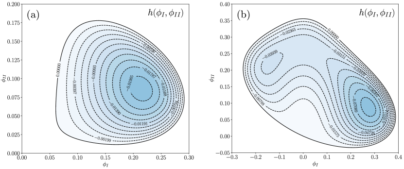
Figure 3: $h(\phi_{\rm I},\phi_{\rm II})$ as obtained for a two-mode approximation of the triangular symmetry with $C=-2.0$ and $D=1.0$ at two quenching depths: (a) $B=0.3$, (b) $B=0.0$. Dashed lines show representative isolines for negative values of $h(\phi_{\rm I},\phi_{\rm II})$.

When considering approximations with more modes, different values of $\phi$ should be considered for every set of amplitudes corresponding to different lengths of $\mathbf{G}_{m}$. Typically this task should be addressed numerically. Consider an approximation with $K$ equal to the number of the modes of different length (under approximations introduced in Sec. 2.3.1). In this case the following function must be minimized,

$$h[\{\phi_{k}\}]=\sum_{k=1}^{K}\bigg{[}BM_{k}\phi_{k}^{2}-\frac{3}{2}DM_{k}\phi_{k}^{4}\bigg{]}+3D\left(\sum_{k=1}^{K}M_{k}\phi_{k}^{2}\right)^{2}+\frac{C}{3}\zeta_{3}(\{\phi_{k}\})+\frac{D}{4}\zeta_{4}^{\rm s}(\{\phi_{k}\}).$$ (38)

with $M_{k}$ the number of reciprocal space vectors for each considered mode (the solid arrows in Fig. 2). For instance, for the three-mode approximation of a cubic lattice in Fig. 2, we would have $M_{1}=2$, $M_{2}=2$ and $M_{3}=4$. $\zeta_{3}(\{\phi_{k}\})$, $\zeta_{4}^{\rm s}(\{\phi_{k}\})$ are the symmetry-dependent polynomials resulting by substituting $\eta_{j}$ with the amplitude associated to the length of the reciprocal space vector they correspond to. To introduce an explicit example, consider the two mode approximation of the triangular symmetry (see Fig. 2(a)), i.e. $\{\phi_{k}\}=[\phi_{I},\phi_{\rm II}]$, $M_{\rm I}=M_{\rm II}=3$, and $\zeta_{3}(\phi_{\rm I},\phi_{\rm II})$, $\zeta_{4}^{\rm s}(\phi_{\rm I},\phi_{\rm II})$ the polynomial resulting by setting $\eta_{j}=\phi_{I}$ for $j=1,2,3$ and $\eta_{j}=\phi_{\rm II}$ for $j=4,5,6$ in Eq. (30). Plots of $h(\phi_{\rm I},\phi_{\rm II})$ for selected parameters ($C=-2.0$ and $D=1.0$) are shown in Fig. 3. At a value $B=0.3$ (Fig. 3(a)), relatively close to the solid-liquid phase transition, the free energy has a single minimum corresponding to $\phi_{\rm I}\approx 0.274$ and $\phi_{\rm II}\approx 0.087$. By increasing the quenching depths, the global minimum shifts to $\phi_{I}\approx 0.215$ and $\phi_{\rm II}\approx 0.086$ for $B=0.0$. Moreover, another relative minimum appears (see Fig. 3(b)), which corresponds to a graphene-like phase. Some extended discussions on all the possible phases which can be described in two dimensions with combination of more modes can be found in Ref. [62].

2.4 Amplitude XPFC

A formulation based on the the so-called structural PFC (XPFC) [20, 21], describing more detailed features and phenomena in crystalline systems such as, e.g. multicomponent systems, structural transformations, anisotropies, and extended defects [63, 11, 58], has been proposed in Ref. [58]. In a dimensionless form, the XPFC free energy $F_{\rm X}$ reads

$$F_{X}=\int\text{d}\mathbf{r}\left[F_{\rm ex}+\frac{n^{2}}{2}-P\frac{n^{3}}{3}+Q\frac{n^{4}}{3}\right],\qquad F_{\rm ex}=-\frac{n(\mathbf{r})}{2}\int\text{d}\mathbf{r}^{\prime}X_{2}(|\mathbf{r}-\mathbf{r}^{\prime}|)n(\mathbf{r}^{\prime}),$$ (39)

where $P$ and $Q$ are parameters and $X_{2}(|\mathbf{r}-\mathbf{r}^{\prime}|)$ is the direct two-point correlation function at the reference density $n_{\rm o}$. In this approach, this function is typically expressed in the reciprocal space, $\hat{X}_{2}(|\mathbf{k}|)$. Following [58], it may be expressed as an envelope of Gaussian peaks associated with different modes of the periodic density or, in other words, to a family of planes of a crystal structure, [21]

$$\hat{X}_{2,j}=\rme^{-\frac{1}{2w_{j}^{2}}(k-{k}_{j})^{2}-\frac{\sigma^{2}}{p_{j}a_{j}}k_{j}^{2}},$$ (40)

where $w_{j}$ controls the elastic and surface energies (the width of the $j$-th Gaussian peak), $\sigma$ is an effective temperature parameter [64], $p_{j}$ and $a_{j}$ are the planar and atomic densities associated with the family of planes corresponding to the $j$-th mode, respectively, while $k_{j}$ is the inverse of the interplanar spacing for the $j$-th family of planes. Then, by assuming an amplitude formulation and volume average as in Sects 2.2–2.3, the polynomial in $n$ that enters $F_{X}$ leads to terms similar to the energy in Eq. (15) except for the excess term which becomes [58]

$$\begin{split}F_{\rm ex,\eta}=\int\text{d}\mathbf{r}\bigg{[}\sum_{m}^{M}&-\frac{\eta_{m}^{*}}{2}\mathcal{F}^{-1}\bigg{\{}\hat{X}_{2}(|\mathbf{k}+\mathbf{G}_{m}|)\hat{\eta}_{m}(\mathbf{k})\bigg{\}}\\ &-\frac{n_{\rm o}}{2}\mathcal{F}^{-1}\bigg{\{}\hat{\xi}_{V}(\mathbf{k})\hat{X}_{2}(|\mathbf{k}|)\hat{n}_{\rm o}(\mathbf{k})\bigg{\}}+\text{c.c.}\bigg{]},\end{split}$$ (41)

where the hat symbol denotes the Fourier transform, $\mathcal{F}^{-1}$ the inverse Fourier transform, and $\hat{\xi}_{V}$ an averaging (convolution) kernel in Fourier space that restricts the wave number to small values, approximately approaching the extension of the first Brillouin zone, which filters out spatial variations smaller than the lattice spacing. Interestingly, this model has been proposed with an ansatz for the amplitude expansion encoding different (two) lattice symmetries (see Sec. 6.4). This ansatz is expected to work with other forms of the energy and it consists just of a different formulation for Eq. (17) leading to results that may be formulated in terms of the equations reported in Sec. 2.3.

3 Numerical methods

In this section, two standard methods (finite difference and spectral) for solving first order in time partial differential equations that are applicable to APFC models are described. Following this, a finite element approach for solving APFC models is outlined and the description of a mesh refinement algorithm is reported.

3.1 Finite differences

In general there are many methods for solving an equations of the form

$$\frac{\partial\psi}{\partial t}=H(\psi),$$ (42)

where $H(\psi)$ is a function of $\psi$. To solve it numerically it is useful to first consider integrating the equation over time from $t$ to $t+\Delta t$ to obtain,

$$\psi(t+\Delta t)=\psi(t)+\int_{t}^{t+\Delta t}\text{d}t^{\prime}\,H(\psi).$$ (43)

The main question is how to approximate the integral in the above equation. In explicit methods only prior knowledge of $\psi$ and its derivatives are used, i.e.,

$$\psi(t+\Delta t)=\psi(t)+\int_{t}^{t+\Delta t}\text{d}t^{\prime}\,\left[H(t)+\left.\frac{\partial H}{\partial t^{\prime}}\right|_{t}t^{\prime}+\frac{1}{2!}\left.\frac{\partial^{2}H}{\partial t^{\prime 2}}\right|_{t}t^{\prime 2}+\cdots\right].$$ (44)

where $H(t)=H(\psi(t))$. The simplest method, Euler’s method, just retains the first term in the expansions, i.e.,

$$\psi(t+\Delta t)=\psi(t)+\Delta tH(t).$$ (45)

This approach must be supplemented by methods to evaluate spatial gradients in $H$, which in (A)PFC type models are typically even order derivatives, i.e., $\nabla^{2},\nabla^{4},\dots$. Often these are evaluated using a central difference formula. For instance, in two dimensions with a 5-points stencil (quincunx), the Laplacian is given by

$$\nabla^{2}f=\frac{f(i+1,j)+f(i,j+1)+f(i-1,j)+f(i,j-1)-4f(i,j)}{\Delta s^{2}},$$ (46)

where $(x,y)=(i\Delta s,j\Delta s$). Eq. (46), in conjunction with Eq. (45), is quite simple to implement for numerical integrations. Moreover, it is easy to incorporate different boundary conditions. However, the time step $\Delta t$ is limited by the grid spacing due to stability constraints, typically

$$\Delta t<\alpha\Delta s^{-k},$$ (47)

where $k$ is the highest order spatial derivative (i.e., $k=6$ for the PFC equation) and $\alpha$ is a constant that is model specific. If $\Delta t$ is too large, the solution very rapidly diverges (a pitchfork instability). The specifics of the origin of this instability are described in detail in Ref. [48]. It is possible to slightly reduce this instability by including next nearest neighbours as done by Oono and Puri [65]. This limitation is quite severe in PFC and APFC models as $k=6$ in the former case and $k=4$ in the latter. This instability can be avoided using semi-implicit approaches that are typically done in Fourier space. However, implicit or more generally semi-implicit approaches may be exploited, evaluating terms in the integrals in Eq. (44) within the range $[t,t+\Delta t]$, to have more stable numerical schemes (see also Sec. 3.3). Also, finite difference approaches may be combined with spatial adaptivity which may allow for efficient simulations (see also Sect. 3.4). A few examples of APFC numerical simulations performed with finite differences can be found, e.g., in Refs. [22, 66, 49, 67, 68, 69, 70]. Alternatively, the instability mentioned above can be avoided using spectral methods, as discussed in the next section.

3.2 Fourier spectral method

Spectral methods solve differential equations treating variables as a sum of basis functions with coefficients to be computed, i.e., through a global representation. The so-called Fourier spectral method exploits the Fourier transform, typically in its discrete formulation for numerical integrations (therefore often referred to as pseudo-spectral, Fourier method). This method is particularly suited for periodic boundary conditions. A key feature of this approach is that, in the Fourier space, differential operators become algebraic expression of the wave vector, e.g. $\nabla^{2}\psi(t)\rightarrow-|k|^{2}\widehat{\psi}_{k}(t)$, where $\widehat{\psi}_{k}$ is the (discrete) Fourier transform of $\psi$. No finite difference approximations are then required if solving for $\widehat{\psi}_{k}(t)$, and $\psi(t)$ may be then obtained through a (discrete) inverse Fourier transform. Moreover, efficient algorithms exist to compute $\widehat{\psi}_{k}$ from $\psi$ and vice-versa, namely exploiting the Fast Fourier Transform (FFT) algorithm [71]. The adaptation of such approaches to phase field modeling in materials physics can be found in reference [72]. This method generally allows for splitting off the linear term in $H$ and solving that part exactly, i.e.,

$$\frac{\partial\psi}{\partial t}={\cal L}\psi+N(\psi),$$ (48)

where ${\cal L}$ is a linear operator and $N$ is a non-linear function of $\psi$. Indeed, in Fourier space, this would then read

$$\frac{\partial\widehat{\psi}_{k}}{\partial t}={\cal L}_{k}\widehat{\psi}_{k}+\widehat{N}_{k},$$ (49)

with $\widehat{N}_{k}$ the Fourier transform of $N(\psi)$ and ${\cal L}_{k}$ is an algebraic expression of the wave vector. Eq. (49) is an ordinary differential equation with solution

$$\widehat{\psi}_{k}(t)=\rme^{{\cal L}_{k}t}\widehat{\psi}_{k}(0)+\rme^{{\cal L}_{k}t}\int_{0}^{t}\text{d}t^{\prime}\,\rme^{-{\cal L}_{k}t^{\prime}}\widehat{N}_{k}(t^{\prime}).$$ (50)

Typically, the numerical instability in Euler’s method occurs when ${\cal L}_{k}$ is the most negative (i.e., at large wavevectors). However, in this method, $\rme^{{\cal L}_{k}t}$ is very small in this limit so that instability is completely avoided. To complete the picture, the non-linear term must be approximated as was done for $H(\psi)$ in the preceding section. Considering Eq. (50) for $\widehat{\psi}_{k}(t+\Delta t)$ and approximating (explicitly) $\widehat{N}_{k}(t^{\prime})\approx\widehat{N}_{k}(t)$ gives

$$\begin{split}\widehat{\psi}_{k}(t+\Delta t)=\ &\rme^{{\cal L}_{k}\Delta t}\widehat{\psi}_{k}(t)+\rme^{{\cal L}_{k}(t+\Delta t)}\int_{t}^{t+\Delta t}\text{d}t^{\prime}\,\rme^{-{\cal L}_{k}t^{\prime}}\widehat{N}_{k}(t^{\prime})\\ \approx\ &\rme^{{\cal L}_{k}\Delta t}\widehat{\psi}_{k}(t)+\frac{\rme^{{\cal L}_{k}\Delta t}-1}{{\cal L}_{k}}\widehat{N}_{k}(t),\end{split}$$ (51)

while other approximations of $\widehat{N}(t^{\prime})$ may be considered as well. Eq. (51) provides a relatively simple method of updating the field $\psi$ at one time step, although it requires Fourier transforms of $\psi$ and $N(\psi)$ and an inverse Fourier transform of $\widehat{\psi}_{k}$ per time step. While the method eliminates the Euler instability, the free energy will increase if the time step is too large, which should not occur. Nevertheless, depending on the specific model, it is possible to use time steps that are tens or hundreds of times larger than those used in the Euler algorithm. For the amplitude expansion, this method is directly applicable as the linear pieces of the equations of motion for $\eta_{m}$ are not coupled to any other amplitudes. Representative examples of APFC numerical simulations exploiting the Fourier pseudo-spectral method can be found, e.g., in Refs. [9, 28, 29, 62, 58, 59, 73, 74, 75, 76].

3.3 Finite element method

The Finite Element Method (FEM) emerged as a particularly suitable framework for solving the APFC model’s equations [60, 77, 16, 78], besides being also employed in PFC studies in the first place [79, 80, 81, 82, 83]. Indeed, it conveniently discretizes partial differential equations (PDEs) while exploiting inhomogeneous and adaptive meshes.

Within FEM, the PDEs are expressed in an integral form (weak form) over their domain of definition ($\Omega$), typically having a rectangular/cubic shape. For the discretization of the resulting equations, a conforming triangulation $\mathcal{T}_{h}$ of the domain $\Omega$ is considered, usually with simplex elements $S\in\mathcal{T}_{h}$ (with characteristic size $h$). In the context of APFC simulations, linear elements have been mostly adopted. This means considering a discrete function space of local polynomial of order 1 ($\mathbb{P}_{1}$), namely $\mathcal{V}_{h}^{1}=\{v\in C(\Omega,\mathbb{R}):v|_{S}\in\mathbb{P}_{1}(S,\mathbb{R}),S\in\mathcal{T}_{\rm h}\}$. A function $y\in\mathcal{V}^{1}_{h}$ can be written in terms of a basis expansion $y=\sum_{i}Y_{i}\Xi_{i}$ with real coefficients $Y_{i}$ and basis $\{\Xi_{i}\}$ of $\mathcal{V}_{h}^{1}$. To solve for complex functions, as $\eta_{m}$, their real and imaginary part can be considered as two (real) independent unknowns. Alternatively, complex coefficients with real basis functions may be considered.

The FEM approach which has been used to solve APFC equations as in Eq. (22), features a splitting into two second-order equations for $\partial\eta_{m}/\partial t$ and $\rho_{m}=\mathcal{G}_{m}\eta_{m}$ (with $m=1,...,M$ as in Sec. 2.3) [60, 77]:

$$\begin{split}\frac{\partial\eta_{m}}{\partial t}&=-|\mathbf{G}_{m}|^{2}\bigg{[}A\mathcal{G}_{m}\rho_{m}+B\eta_{m}+3D(\Phi-|\eta_{m}|^{2})\eta_{m}+\frac{\partial f^{\rm s}}{\partial\eta_{m}^{*}}\bigg{]},\\ \rho_{m}&=\mathcal{G}_{m}\eta_{m}=\nabla^{2}\eta_{m}+2{\mathbb{i}}\mathbf{G}_{m}\cdot\nabla\eta_{m}.\end{split}$$ (52)

This choice is convenient within the APFC framework as it allows the computing of relevant quantities straightforwardly as, e.g., the stress field, which may be rewritten in terms of both $\eta_{m}$ and $\rho_{m}$ and their spatial derivatives [16] (see also Sec. 4.2). Moreover, even though it is defined for $\mathcal{G}_{m}$, $\rho_{m}$ can be readily be used for computing $\mathcal{L}_{m}$, for instance when considering multi-mode approximations. From a numerical point of view, the splitting in Eq. (52) allows exploiting linear elements as only second-order operators appear, which translate to first order operators acting on elements of $\mathcal{V}_{h}^{1}$ in the weak form. With $(f,\,g)\coloneqq\int_{\Omega}f(\mathbf{r})g(\mathbf{r})\,\text{d}\mathbf{r}$ the $L^{2}(\Omega,\mathbb{R})$ scalar product, and considering the integral form of Eq. (52), the problem to solve then reads: for $t\in[0,T]$, find $\eta_{m}(t)=a_{m}(t)+{\mathbb{i}}b_{m}(t)$ and $\rho_{m}(t)=c_{m}(t)+{\mathbb{i}}d_{m}(t)$, with $a_{m},b_{m},c_{m},d_{m}\in\mathcal{V}^{1}_{h}$ (implying hereafter their dependence on $t$), such that

$$\begin{split}\left(\frac{\partial a_{m}}{\partial t},\,v\right)-A|\mathbf{G}_{m}|^{2}\bigg{[}(\nabla c_{m},\,\nabla v)+2(\mathbf{G}_{m}\cdot\nabla d_{m},\,v)\bigg{]}&=\left({\rm Re}[H(\{\eta\})],\,v\right),\ \\ \left(\frac{\partial b_{m}}{\partial t},\,v\right)-A|\mathbf{G}_{m}|^{2}\bigg{[}(\nabla d_{m},\,\nabla v)-2(\mathbf{G}_{m}\cdot\nabla c_{m},\,v)\bigg{]}&=\left({\rm Im}[H(\{\eta\})],\,v\right),\ \\ (c_{m},\,v)+(\nabla a_{m},\,\nabla v)+2(\mathbf{G}_{m}\cdot\nabla b_{m},\,v)&=0\ ,\\ (d_{m},\,v)+(\nabla b_{m},\,\nabla v)-2(\mathbf{G}_{m}\cdot\nabla a_{m},\,v)&=0\ ,\end{split}$$ (53)

$\forall v\in\mathcal{V}^{1}_{h}$ subject to an initial conditions $\eta_{m}(0)=\eta_{m}^{0}$, and $H(\{\eta\})$=$\partial f^{\rm s}/\partial\eta_{m}+B\eta_{m}+3D(\Phi-|\eta_{m}|^{2})\eta_{m}$. The time derivatives are approximated by $\partial a_{m}/\partial t=(a_{m}^{j+1}-a_{m}^{j})/\Delta t_{j}$ and $\partial b_{m}/\partial t=(b_{m}^{j+1}-b_{m}^{j})/\Delta t_{j}$, with $\Delta t_{j}=t_{j+1}-t_{j}$ the time step, and $j\in\mathbb{N}_{0}$ the index labelling time steps. The time discretization is obtained through an implicit-explicit (IMEX) scheme. It consists of evaluating all the linear (nonlinear) terms in Eq. (53) implicitly (explicitly), i.e. at time $t^{j+1}$ ($t^{j}$) [60, 77], with $a^{j+1}_{m}$, $b^{j+1}_{m}$, $c^{j+1}_{m}$, $d^{j+1}_{m}$ the unknowns to solve for. Eq. (53) consists of a set of nonlinear equations due to $H(\{\eta\})$. This term can be generally linearized and handled through iterative approaches as Picard Iterations or the Newton method. A simple but effective approach, which can be exploited for methods introduced in previous sections too, consists of applying a one-iteration Newton method [60], i.e. approximating $H(\eta^{j+1})$ as

$$H(\eta^{j+1})=H(\eta^{j})+H^{\prime}(\eta^{j})(\eta^{j+1}-\eta^{j}).$$ (54)

To solve Eq. (53), basis function expansions of unknowns are considered, e.g. $a^{j+1}_{m}=\sum_{i}Y_{m,i}^{j+1}\Xi_{i}$, with ${Y}_{m,i}^{j+1}$ the coefficients to be computed at the $j$-th timestep (and analogous expressions and coefficients’ definition for $b^{j+1}_{m},c^{j+1}_{m},d^{j+1}_{m}$). These coefficients are computed by substituting the basis function expansions into Eq. (53), setting basis functions as test functions, and solving the resulting system of equations. Notice that $M$ coupled systems (53) must be solved concurrently, with $M$ the number of independent amplitudes according to the considered lattice symmetry and approximation (see Sec. 2.3). Boundary conditions (BC) such as Dirichlet, Neumann, or Periodic BC, may be included as in common FEM approaches. Further discussions and explanations of standard aspects can be found in specialized textbooks.

The FEM approach outlined above proved efficient in handling relatively large systems in both two and three dimensions, in combination with standard direct and iterative solvers within FEM toolboxes like, e.g., AMDiS [84, 85]. Further improvements may be devised to increase the performances. An example is reported in [77] where the development of a dedicated preconditioner [86, 87] allowing for fast solver convergence has been proposed and exploited for simulations of hundreds of nanometers domains in three dimensions for some materials.

The approach described in this section is also prone to coupling with other equations. Indeed, other variables would share spatial features with amplitudes. Coupling terms could be considered as additional terms entering $\partial{\eta}_{m}/\partial t$. At the same time, other equations may be discretized readily following the main FEM features described above (linear elements, operator splitting in second-order PDEs, IMEX time discretization). This has been exploited for instance when imposing mechanical equilibrium [16] (see Sec. 5.2), to simulate binary systems [13] (see Sec. 6.3), and to investigate the effect of magnetic field on small-angle grain boundaries [88].

3.4 Mesh adaptivity

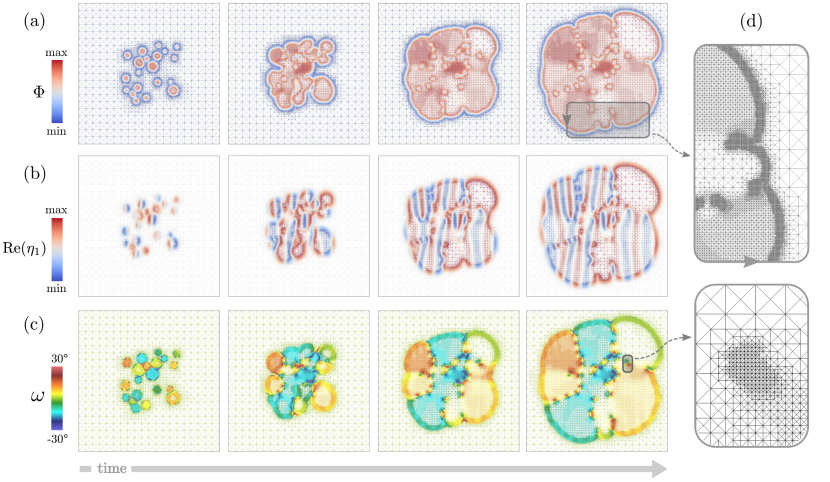
Figure 4: Illustration of the growth of 20 crystal seeds (with a triangular lattice, one-mode approximation) having random orientation ranging in $[-15^{\circ},15^{\circ}]$, as obtained by an APFC simulation with an adaptive mesh. The spatial discretization is represented by means of the mesh while colors represent: (a) $\Phi=\sum_{m}^{M}|\eta_{m}|^{2}$, (b) Re$(\eta_{1})$, as indexed in (29), (c) local rotation $\omega$ w.r.t the reference crystal set by $\mathbf{G}_{m}$, computed by Eq. (69). (d) Magnification of two regions showing the mesh on a smaller length scale at the solid-liquid interface (top) and at a defect (bottom). Reprinted from [77] $\copyright$ IOP Publishing Ltd. All rights reserved.

Exploiting spatial adaptivity is a convenient strategy for performing efficient simulations with the APFC model [66, 60, 67, 77]. Indeed, amplitudes are constant for relaxed crystals, oscillate with different periodicity according to the local distortion of the crystal with respect to the reference one (see, e.g., Fig. 1) and exhibit significant variation at defects and solid-liquid interfaces. Depending on the numerical approach and set of equations, one may devise different strategies to set a local refinement, e.g., based on error estimates or indicators.

An optimized local resolution based on the amplitudes oscillations, which works even for the standard approaches considered so far, has been achieved focusing on phases of the complex amplitudes, $\text{arg}(\eta_{m})=\theta_{m}$. By looking at this quantity, it is possible to determine the wavelength of oscillating amplitudes $\lambda_{m}$ [77]. Then for a good resolution of all the amplitudes, the discretization $h$ should be a fraction of the smallest $\lambda_{m}$, i.e. $h_{\rm amp}=\min_{m}{(\lambda_{m})}/n$, with $n\geq 10$.

To use this criterion in practice, the deformation, strain and/or rotation fields must be derived from amplitudes. This will be discussed in detail in the following section (see Sec. 4.2). In addition to the oscillation of amplitudes, a refinement for the interfaces and defects controlled by $h_{\rm min}$ where $|\nabla\Phi|$ is significantly larger than a relatively small threshold $\varsigma$ and imposed as finest resolution in the mesh is considered [60], while a large discretization bound $h_{\rm max}$ is defined for region where $\Phi\sim 0$ or where $\theta_{m}\rightarrow 0$ (i.e. for constant amplitudes). Summarizing these concepts, this method ensures a local discretization, $h$, as

$$h=\begin{cases}h_{\rm min},&\mbox{if }|\nabla\Phi|\geq\varsigma\\ \min(\hskip 1.0pt\max(h_{\rm amp},h_{\rm min})\hskip 1.0pt,\hskip 1.0pth_{\rm max}\hskip 1.0pt),&\mbox{if }\Phi>0\mbox{ and }|\nabla\Phi|<\varsigma\\ h_{\rm max},&\mbox{elsewhere.}\end{cases}$$ (55)

This approach has been exploited together with the FEM approach outlined in Sec. 3.3, in particular within the FEM toolbox AMDiS [84, 85]. However, it is expected to work with any real-space method readily. Further optimization of the mesh refinement can be achieved by a polar representation [66, 67] which involves, however, some changes in the amplitude equations, the coupling with additional fields, and other technical details to be considered. An examples of an APFC simulation performed with the adaptive refinement strategy here outlined is given in Fig. 4.

4 Continuum limit: elasticity and plasticity

4.1 Elasticity

The elastic properties in the amplitude expansion arise from the term $A\sum_{m}^{M}\Gamma_{m}|\mathcal{G}_{m}\eta_{m}|^{2}$ (see Eq. (28)). Indeed, all the other terms in the free energy do not give rise to gradients in the phase of the amplitudes and as such do not contribute to the elastic energy. To obtain the consequences of this term it is useful to consider deformations ($\mathbf{u}\equiv\mathbf{u}(\mathbf{r})$) from a perfect lattice, i.e.,

$$\eta_{m}=\phi_{m}\rme^{-{\mathbb{i}}\theta_{m}},$$ (56)

where $\theta_{m}\equiv{\bf G}_{m}\cdot\mathbf{u}$ and $\phi_{m}$ is weakly dependent on $\mathbf{u}$ (see a 1D illustration in Fig. 1(b)). This leads to

$$\begin{split}\mathcal{G}_{m}\eta_{m}&=\phi_{m}\,\rme^{-{\mathbb{i}}\mathbf{G}_{m}\cdot\mathbf{u}}\left(-{\mathbb{i}}\nabla^{2}\theta_{m}-|\nabla\theta_{m}|^{2}+2\mathbf{G}_{m}\cdot\nabla\theta_{m}\right)\\ &\approx\phi_{m}\,\rme^{-{\mathbb{i}}\mathbf{G}_{m}\cdot\mathbf{u}}\left(-|\nabla\theta_{m}|^{2}+2\mathbf{G}_{m}\cdot\nabla\theta_{m}\right),\end{split}$$ (57)

where in the last line higher order gradients in $\mathbf{u}$ have been neglected. So that

$$\begin{split}\sum_{m}^{M}\Gamma_{m}|\mathcal{G}_{m}\eta_{m}|^{2}&=4\sum_{m}^{M}\Gamma_{m}\phi_{m}^{2}G_{i}^{m}G_{j}^{m}G_{k}^{m}G_{l}^{m}\left(u_{ij}u_{kl}-u_{ij}u_{ko}u_{lo}+\frac{1}{4}u_{io}u_{jo}u_{kp}u_{lp}\right),\end{split}$$ (58)

where $u_{ij}\equiv\partial u_{i}/\partial x_{j}$, $G_{i}^{m}$ is the $i$-th component of $\mathbf{G}_{m}$ and the Einstein summation convention is used. Eq. (58) contains linear and non-linear terms. In terms of the non-linear Eulerian-Almanasi strain measure (${\bf U}$) [57, 73] with elements ,

$$U_{ij}=\frac{1}{2}\left(u_{ij}+u_{ji}-u_{ik}u_{jk}\right),$$ (59)

Eq. (58) can be written as

$$\sum_{m}^{M}\Gamma_{m}|\mathcal{G}_{m}\eta_{m}|^{2}=4\sum_{m}^{M}\Gamma_{m}\phi_{m}^{2}G_{i}^{m}G_{j}^{m}G_{k}^{m}G_{l}^{m}U_{ij}U_{kl}.$$ (60)

The elastic part of the free energy is then

$$F_{\rm elas}=\frac{1}{2}\int d\mathbf{r}\ [\sigma_{ij}U_{ij}]=4A\int d\mathbf{r}\bigg{[}\sum_{m}^{M}\Gamma_{m}\phi_{m}^{2}G_{i}^{m}G_{j}^{m}G_{k}^{m}G_{l}^{m}U_{ij}U_{kl}\bigg{]}.$$ (61)

The components of the stress tensor defined as

$$\sigma_{ij}=\mathcal{C}_{ijkl}U_{kl},$$ (62)

where $\mathcal{C}_{ijkl}$ is the elastic modulus tensor [94] are then given by

$$\mathcal{C}_{ijkl}=8A\sum_{m}^{M}\Gamma_{m}\phi_{m}^{2}G_{i}^{m}G_{j}^{m}G_{k}^{m}G_{l}^{m}.$$ (63)

Thus Eq. (63) provides a general formula for the elastic moduli for arbitrary crystal symmetry. Some specific examples are given below.

Examples:

For a free energy with a single mode, i.e., containing the term $n(1+\nabla^{2})^{2}n/2$, 2D triangular and 3D BCC structures minimize the free energy in certain parameter ranges. At a minimum these systems can be described by modes with the same length scale and thus $\Gamma_{m}=1$ and $\phi_{m}=\phi$, $\forall m$. Following the definition of $\mathbf{G}_{m}$ as in Sec. 2.3.2 for these symmetries (one-mode approximation), Eq. (61) gives

$$\begin{split}F^{\rm TRI}_{\rm elas}=&A\phi^{2}\int\text{d}\mathbf{r}\bigg{[}\frac{9}{2}\sum_{i}U_{ii}^{2}+3U_{xx}U_{yy}+6U_{xy}^{2}\bigg{]},\\ F_{\rm elas}^{\rm BCC}=&A\phi^{2}\int\text{d}\mathbf{r}\bigg{[}4\sum_{i}U_{ii}^{2}+4\sum_{i,j>i}U_{ii}U_{jj}+8\sum_{i,j>i}U_{ij}^{2}\bigg{]}.\end{split}$$ (64)

For the FCC symmetry in the two-mode approximations (see Sec. 2.3.2), $\Gamma_{m}=1/16$, $\forall m$. This gives

$$F_{\rm elas}^{\rm FCC}=\frac{A}{9}\int\text{d}\mathbf{r}\bigg{[}(\phi^{2}+4\psi^{2})\sum_{i}U_{ii}^{2}+2\phi^{2}\sum_{i,j>i}U_{ii}U_{jj}+4\phi^{2}\sum_{i,j>i}U_{ij}^{2}\bigg{]},$$ (65)

where $\eta_{m}=\phi\rme^{-{\mathbb{i}}\theta_{m}}$ for $i=1,...,4$ and $\eta_{m}=\psi\rme^{-{\mathbb{i}}\theta_{m}}$ for $i=5,...,7$.

One of the difficulties in parameterizing PFC models is that the ratio of the elastic moduli cannot be changed in the one mode triangular and BCC cases. However, it is interesting to note that in the FCC case, the ratio of the elastic moduli depends on $\psi$, which in principle can be tuned. It suggests that adding more length scales will allow for more tuneability in the models as shown in XPFC models [21]. However, it is important to note that if the added vectors have the same symmetry as the original ones this will not change the ratios.

4.2 Strain and stress field from the amplitudes

When examining the results of APFC simulations, it is useful to develop methods to extract the strain and stress fields directly from the complex amplitudes. As shown by Salvalaglio et al[14] the displacement field, $\mathbf{u}$ that enters continuum elasticity field can be extracted directly from the phase of the amplitudes ($\theta_{m}$). In two dimensions (2D), inverting Eq. (56), the expression is

$$u^{\rm 2D}_{i}=-\frac{\epsilon_{ij}}{\hat{\mathbf{p}}\cdot(\mathbf{G}_{l}\times\mathbf{G}_{m})}\big{[}G_{j}^{m}\theta_{l}-G_{j}^{l}\theta_{m}\big{]},$$ (66)

with $(i,j)=(x,y)$ and cyclic permutations, $\epsilon_{ij}$ is the 2D Levi-Civita symbol, $l$ and $m$ label two different amplitudes, $\hat{\mathbf{p}}=\hat{\mathbf{x}}\times{\hat{\mathbf{y}}}$ the normal vector of the xy-plane and $\theta_{m}=\arg({\eta_{m}})=\arctan\left[\text{Im}(\eta_{m})/\text{Re}(\eta_{m})\right]$. In three dimensions (3D) it can be shown that

$$\begin{split}u_{i}^{\rm 3D}=-\frac{1}{\mathbf{G}_{n}\cdot(\mathbf{G}_{m}\times\mathbf{G}_{l})}\big{[}&\theta_{l}(G_{k}^{m}G_{j}^{n}-G_{j}^{m}G_{k}^{n})+\theta_{m}(G_{k}^{n}G_{j}^{l}-G_{j}^{n}G_{k}^{l})\\ &+\theta_{n}(G_{k}^{l}G_{j}^{m}-G_{j}^{l}G_{k}^{m})\big{]}.\end{split}$$ (67)

with $(i,j,k)=(x,y,z)$ and cyclic permutations, and $l$, $m$, $n$, labelling three different amplitudes. These quantities are discontinuous. However the component of the (linear) strain tensor $\mathbf{U}^{\rm L}$ become expressions of $\partial\theta_{m}/\partial x_{i}$ with

$$\frac{\partial\theta_{m}}{\partial x_{i}}=\frac{1}{|\eta_{m}|^{2}}\left[\frac{\partial\text{Im}(\eta_{m})}{\partial x_{i}}\text{Re}(\eta_{m})-\frac{\partial\text{Re}(\eta_{m})}{\partial x_{i}}\text{Im}(\eta_{m})\right],$$ (68)

which is continuous almost everywhere in the solid phase, with a singularity for vanishing amplitudes in correspondence of phase singularities, e.g., at the cores of defects. Then, with a regularization for these amplitudes (see also Sec. 4.4), elastic field can be readily computed and conveniently exploited. In two dimensions, for $\mathbf{U}^{\rm L}$ and the rotation field $\omega=\nabla\times\mathbf{u}$ we then get

$$\begin{split}U_{xx}^{\rm L}&=-\frac{1}{\hat{\mathbf{p}}\cdot(\mathbf{G}_{l}\times\mathbf{G}_{m})}\left(G_{y}^{m}\frac{\partial\theta_{l}}{\partial x}-G_{y}^{l}\frac{\partial\theta_{m}}{\partial x}\right),\\ U_{yy}^{\rm L}&=-\frac{1}{\hat{\mathbf{p}}\cdot(\mathbf{G}_{l}\times\mathbf{G}_{m})}\left(G_{x}^{l}\frac{\partial\theta_{m}}{\partial y}-G_{x}^{m}\frac{\partial\theta_{l}}{\partial y}\right),\\ U_{xy}^{\rm L}&=-\frac{1}{2\hat{\mathbf{p}}\cdot(\mathbf{G}_{l}\times\mathbf{G}_{m})}\left(G_{y}^{m}\frac{\partial\theta_{l}}{\partial y}-G_{y}^{l}\frac{\partial\theta_{m}}{\partial y}+G_{x}^{l}\frac{\partial\theta_{m}}{\partial x}-G_{x}^{m}\frac{\partial\theta_{l}}{\partial x}\right),\\ \omega&=-\frac{1}{2\hat{\mathbf{p}}\cdot(\mathbf{G}_{l}\times\mathbf{G}_{m})}\left(G_{y}^{m}\frac{\partial\theta_{l}}{\partial y}-G_{y}^{l}\frac{\partial\theta_{m}}{\partial y}-G_{x}^{l}\frac{\partial\theta_{m}}{\partial x}+G_{x}^{m}\frac{\partial\theta_{l}}{\partial x}\right).\end{split}$$ (69)

Explicit expressions for 3D strain and rotation fields can be found in Ref. [14]. The stress field can then be computed through the Hooke’s law (62).

In 2018 Skaugen, Angheluta and Viñals [12] derived an expression for the stress tensor, $\sigma_{ij}$ from the density field using the standard definition of $\sigma_{ij}$, i.e,

$$\sigma_{ij}=\frac{\delta\Delta F}{\delta(\partial_{i}u_{j})},$$ (70)

where $\Delta F=F(n(\mathbf{r}+\mathbf{u}))-F(n(\mathbf{r}))$ and $\mathbf{u}$ is the displacement field. This gives

$$\sigma_{ij}=[\partial_{i}{\cal L}n]\partial_{j}n-[{\cal L}n](\partial_{ij}n)+P\delta_{ij},$$ (71)

where $P=f-n(\delta F/\delta n)$ is a pressure term summing up to the mechanical stress, with $f$ the integrand in Eq. (1), the second term arising when considering mass-conserving deformations [95], and ${\cal L}\equiv 1+\nabla^{2}$. In terms of amplitudes, integrating over the a unit cell with $n$ expressed via Eq. (17) and neglecting the pressure terms gives [16]

$$\begin{split}\sigma_{ij}=\sum_{m}^{M}&\bigg{\{}\big{[}(\partial_{i}+{\mathbb{i}}G_{i}^{m})(\nabla^{2}+2{\mathbb{i}}\mathbf{G}_{m}\cdot\nabla)\eta_{m}\big{]}\big{[}(\partial_{j}-{\mathbb{i}}G_{j}^{m})\eta_{m}^{*}\big{]}\\ &-\big{[}(\nabla^{2}+2{\mathbb{i}}\mathbf{G}_{m}\cdot\nabla)\eta_{m}\big{]}\big{[}(\partial_{i}-{\mathbb{i}}G_{i}^{m})(\partial_{j}-{\mathbb{i}}G_{j}^{m})\eta_{m}^{*}+\text{c.c.}\big{]}\bigg{\}},\end{split}$$ (72)

for one-mode approximations, while it can be generalized for more modes accounting for the full ${\cal L}_{m}$ operators (see Eq. (20)).

4.3 Plasticity and defect dynamics

As seen in previous sections, the amplitude formalism can describe the elastic behavior of crystals as encoded in the PFC model. Moreover, by focusing on singularities in the corresponding phases, the motion of defects may be connected to the evolution amplitudes [15, 12, 13, 96].

A dislocation in a crystalline lattice corresponds to a discontinuity in the phase $\theta_{m}$. At the same time, a dislocation with Burgers vector $\mathbf{b}$ is defined by $\oint d\mathbf{u}=\mathbf{b}$ [97], thus it can be shown that $\oint\text{d}\theta_{m}=-\mathbf{G}_{m}\cdot\mathbf{b}=-2\pi s_{m}$, where $s_{m}$ is the winding number. As discussed in Ref. [12], a vortex solution for amplitudes at dislocation cores may be assumed, that reads $\eta_{m}\propto x-{\mathbb{i}}s_{m}y$ with $s_{m}=\pm 1$. The Burgers vector distribution of a dislocation can be defined as a localized (vectorial) topological charge $\mathbf{b}\delta(\mathbf{r}-\mathbf{r}_{0})$ with $\mathbf{r}_{0}$ the nominal position of the dislocation core, assumed pointwise from a continuous point of view. By extension, the Burgers vector density can be defined to be $\mathbf{B}(\mathbf{r})=\sum_{d=1}^{D}\mathbf{b}^{d}\delta(\mathbf{r}-\mathbf{r}^{d}_{0})$, with $d$ indexing the dislocations and $D$ their total number. To connect this quantity to amplitudes, note that the position of the core is where the amplitudes go to zero. Therefore, following the theoretical framework reported in [98, 99, 100], a change of coordinates from the canonical one to the amplitudes’ components can be considered. Namely, for point dislocations in two dimensions, or straight dislocations in three dimensions, one gets

$$\mathbf{B}(\mathbf{r})=-\beta\sum_{m}^{M}\mathbf{G}_{m}D_{m}\delta(\eta_{m}),\quad D_{m}=\frac{\epsilon_{ij}}{2{\mathbb{i}}}\partial_{i}\eta^{*}_{m}\partial_{j}\eta_{m},$$ (73)

with $D_{m}$ the Jacobian determinant of the coordinates’ transformation, $\beta\equiv\beta_{k}=2\pi/\sum_{m}^{M}(G^{m}_{k})^{2}$ as $\beta_{x}=\beta_{y}=\beta_{z}$ (as can be verified explicitly with $\mathbf{G}_{m}$ defined in Sec. 2.3.2), $\epsilon_{ij}$ is the Levi-Civita symbol, delta functions transforming as $D_{m}\delta(\eta_{m})=-(2\pi)^{-1}\sum_{d}^{D}(\mathbf{q}_{m}\cdot\mathbf{b}^{d})\delta(\mathbf{r}-\mathbf{r}^{d}_{0})$ [98, 99, 12], and implying the Einstein summation convention. Aiming at the velocity of dislocations, the dynamics of $\mathbf{B}(\mathbf{r})$ is considered. Exploiting that the determinant fields $D_{m}$ have conserved currents [100], $\partial D_{m}/\partial t=-\partial_{i}J_{i}^{m}$, with

$$J^{m}_{i}=\epsilon_{ij}\text{Im}\left(\frac{\partial\eta_{m}}{\partial t}\partial_{j}\eta_{m}^{*}\right),$$ (74)

and that a similar continuity equation holds true for $\delta(\eta_{m})$, from Eq. (73) the equation of motion for $B_{i}$ may be written,

$$\begin{split}\frac{\partial B_{i}}{\partial t}=&-\partial_{j}{\cal J}_{ij}=-\partial_{j}\bigg{[}\beta\sum_{m}^{M}G_{i}^{m}J_{j}^{m}\delta(\eta_{m})\bigg{]}\\ =&\ \partial_{j}\bigg{[}\frac{\beta}{2\pi}\sum_{m}^{M}G_{i}^{m}J_{j}^{m}\sum_{d}^{D}\frac{\mathbf{G}_{m}\cdot\mathbf{b}^{d}}{D_{m}}\delta(\mathbf{r}-\mathbf{r}_{0}^{d})\bigg{]},\end{split}$$ (75)

where the last term was obtained by transforming back the delta function to spatial coordinates. For dislocations moving at a velocity $\mathbf{v}^{d}$, it also follows that ${\cal J}_{ij}=\sum_{d}^{D}b_{i}^{d}v_{j}^{d}\delta(\mathbf{r}-\mathbf{r}^{d}_{0})$. Therefore, by equating this latter expression with the corresponding quantity in Eq. (75), the dislocation velocity can be related to the evolution of amplitudes as

$$\mathbf{v}^{d}=\frac{\beta}{2\pi}\sum_{m}^{M}\frac{(\mathbf{G}_{m}\cdot\mathbf{b}^{d})^{2}}{|\mathbf{b}^{d}|^{2}}\frac{\mathbf{J}_{m}}{D_{m}}.$$ (76)

At the dislocation core, a few simplifications may be considered. For the amplitudes which are zero at the dislocation core,

$$\frac{\partial\eta_{m}}{\partial t}=-|\mathbf{G}_{m}|^{2}A\Gamma_{m}{\cal G}_{m}^{2}\eta_{m}\approx-{\mathbb{i}}8A\Gamma_{m}|\mathbf{G}_{m}|^{2}(\mathbf{G}_{m}\cdot\nabla\phi_{m})\left(\mathbf{G}_{m}\cdot\nabla\theta_{m}\right)\rme^{{\mathbb{i}}\theta_{m}},$$ (77)

while others do not contribute to Eq. (76). The latter term in Eq. (77) is obtained by imposing again a form for amplitudes as in Eq. (56) and retaining the lowest order only in $\phi_{m}$ and $\theta_{m}$. Combing all the equations reported above gives

$$v_{i}^{d}=\frac{8\beta Ab_{j}^{d}}{|\mathbf{b}^{d}|^{2}}\epsilon_{ik}\sum_{m}^{M}\Gamma_{m}|\mathbf{G}_{m}|^{2}G_{j}^{m}G_{k}^{m}G_{l}^{m}G_{p}^{m}U_{lp}.$$ (78)

where $U_{ij}=(\partial_{i}u_{j}+\partial_{j}u_{i})/2$. This equation is consistent with the classical Peach-Koehler force [97]. For the case of a 2D triangular lattice or a 3D BCC crystal where it is possible to construct the lattice by retaining only one mode of the lowest order (with $|\mathbf{G}_{m}|=1$, $\Gamma_{m}=1$), the velocity takes the form

$$v_{i}^{d}=M\epsilon_{ij}\left(\sigma_{jk}b_{k}^{d}\right),$$ (79)

with M a mobility factor.

With this formalism, the dynamic of defects may be obtained once $\partial{\eta_{m}}/\partial{t}$ are known. This applies independently to the specific contributions affecting the dynamics of amplitudes. See, for instance, an application to binary systems in Sec. 6.3. The equations presented here apply for point dislocations in two dimensions or straight dislocations in three dimensions. A generalization to curved dislocations in three dimensions has been recently introduced in Ref. [96].

4.4 Comparisons with elasticity theories

As noted in previous sections, the APFC model may be employed to the study elasticity and plasticity in crystalline systems. A few prototypical cases have been investigated, delivering direct comparisons with predictions from other theories [101, 14, 16]. Of particular note is the comparison with continuum elasticity results, as the coarse-grained nature of APFC may deliver advanced/improved continuum approaches.

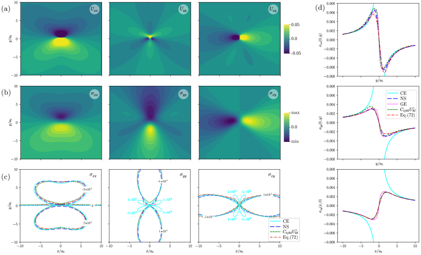
Figure 5: Elastic field induced by an edge dislocation in a 2D triangular lattice (one-mode approximation) with $b=a_{0}=4\pi/\sqrt{3}$. Parameters for the considered APFC simulation: $A=0.98$, $B=0.044$, $C=-0.5$, $D=1/3$. (a) Strain field $U_{ij}^{\rm L}$ from Eqs. (69) with $l=1$ and $m=3$, i.e. the amplitudes with singular phases. (b) Stress field from Eqs. (72). (c) Comparison of representative isolines of the 2D stress fields obtained by different methods and continuum theories: Eq. (62) with $U_{ij}^{\rm L}$ as in panel (a), stress fields from panel (b), classical continuum elasticity from Eq. (81) with $c=0$ (CE), non-singular field theory from Eq. (81) with $c=a_{0}$ (NS). (d) Comparison of stress fields as in panel (c) along a line crossing the defect core, including also the stress field from the strain gradient formulation of Eq. (82) (GE).

A representative case is the elastic field generated by dislocations at mechanical equilibrium, which is well known in the continuum (linear) elasticity for isotropic media [97, 102]. In the APFC model, configurations with dislocations in prescribed positions may be obtained with different approaches. The phase of amplitudes $\sigma_{\texttt{h}\texttt{k}\texttt{l}}$ can be initialized with singularities as discussed in Sec. 4.3 at given positions and then the APFC model is used to minimize the free energy. By restricting the description to 2D crystals for the sake of simplicity, a convenient approach consists of setting phases $\theta_{m}=-\mathbf{G}_{m}\cdot\mathbf{u}^{\rm dislo}$ with

$$\begin{split}u_{x}^{\rm dislo}&=\frac{b}{2\pi}\bigg{[}\arctan{\left(\frac{y}{x}\right)}+\frac{xy}{2(1-\nu)(x^{2}+y^{2})}\bigg{]},\\ u_{y}^{\rm dislo}&=-\frac{b}{2\pi}\bigg{[}\frac{(1-2\nu)}{4(1-\nu)}\log{\left(x^{2}+y^{2}\right)}+\frac{x^{2}-y^{2}}{4(1-\nu)(x^{2}+y^{2})}\bigg{]},\\ \end{split}$$ (80)

the displacement field of an edge dislocation having Burgers vector $\mathbf{b}=b\hat{\mathbf{x}}$ and $\nu$ the Poisson’s ratio [97]. Alternatively, an initial strain that induces the formation of dislocations can be considered. For instance, a pair of dislocations having the Burgers vector $\pm\mathbf{b}^{\rm edge}$ is obtained by defining layers with initial deformation $\mathbf{u}=[Dx,0]$ with $D=\pm b/L$ and allowing the system to relax [60]. Dislocations move when Peach-Koehler force is finite assuming no barriers exist (see Sec. 5.4). As discussed in Sec. 5.2, for dynamical configurations, corrections are needed to account for mechanical equilibrium within (A)PFC. Special cases are the configurations where defects do not move, and relaxation given by dynamical equations effectively approaches mechanical equilibrium. These may be represented, for example, by equally spaced arrays of dislocations along $\hat{\mathbf{x}}$ and $\hat{\mathbf{y}}$ with alternating Burgers vectors, i.e., a “grid” where four defects with the same Burgers vectors surround another one with opposite Burgers vector. It is worth mentioning that a single dislocation, in the absence of external stress, would be in principle stationery too (as the Peach-Koehler force is zero). Still, its elastic field would inherently interact with the boundaries of any finite simulation domain as it is long-range, with energy dependent on the system size and diverging for an infinite medium. A possible solution would be studying a single dislocation in a finite crystal [16], which, however, is expected to induce changes in the elastic field [97, 103, 104].

Fig. 5 shows the elastic field of a dislocation belonging to a two dimensional grid with alternating Burgers vector along $\hat{\mathbf{x}}$ and $\hat{\mathbf{y}}$. Both strain components resulting from computing Eqs. (69) (Fig. 5(a)) and stress components from Eq. (72) (Fig. 5(b)) are shown. These fields agree well with the field expected in classical continuum elasticity [97]. The elastic field obtained from Eqs. (69) is to some extent easier to compute as it involves only the first derivatives of amplitudes. Still, they are singular at the core of vanishing amplitudes, here regularized by setting to $1/(|\eta_{m}|^{2}+\delta)$ with a small $\delta$ as prefactor in Eq. (68). On the other hand, the elastic field from Eq. (72) does not require such a numerical regularization. This approach involves higher-order derivatives than Eq. (68), which can be handled efficiently when combined with a proper splitting of the APFC equations (see also Sec. 3).

More insights are given in Fig. 5(c) and Fig. 5(d). Therein, a comparison of the stress field components obtained with different continuum theories for representative isolines (panel c) and along lines crossing the defect core (panel d) is reported. In particular, it shows the stress fields components computed from the APFC simulation, namely Eq. (72) and Eq. (62) with $U_{ij}^{\rm L}$ from Eq. (69) with $\phi^{2}=\sum_{m=1}^{3}|\eta_{m}|^{2}/3$. These fields are compared with the non-singular isotropic theory (NS) reported by Wei Cai et alin Ref. [102],

$$\frac{\sigma_{xx}^{\rm NS}}{\sigma_{0}}=-\frac{y(3c^{2}+3x^{2}+y^{2})}{(c^{2}+x^{2}+y^{2})^{2}},\ \ \frac{\sigma_{yy}^{\rm NS}}{\sigma_{0}}=-\frac{y(c^{2}-x^{2}+y^{2})}{(c^{2}+x^{2}+y^{2})^{2}},\ \ \frac{\sigma_{xy}^{\rm NS}}{\sigma_{0}}=\frac{x(c^{2}+x^{2}-y^{2})}{(c^{2}+x^{2}+y^{2})^{2}},$$ (81)

and $\sigma_{zz}^{\rm NS}=\nu(\sigma_{xx}^{\rm NS}+\sigma_{yy}^{\rm NS})$, with $\sigma_{0}=Eb_{x}/(4\pi(1-\nu)^{2})$, $E$ the Young modulus, $\nu$ the Poisson ratio, and $c$ a parameter controlling the extension of the core-regularization ($c=0$ reduces to classical continuum elasticity (CE) formulations $\sigma^{\rm CE}$ [97]). The triangular symmetry considered here, which results isotropic, and under the plane strain condition, gives $\upmu=\uplambda=3\phi^{2}$ while $E=\upmu(3\uplambda+2\upmu)/(\uplambda+\upmu)=(5/2)\phi^{2}$, and $\nu=\uplambda/(2\uplambda+2\upmu)=1/4$ . Another comparison with continuum elasticity is provided with a regularized formulation of the stress emerging in the framework of strain-gradient elasticity (Helmholtz type) [105, 106]

$$\begin{split}\frac{\sigma_{xx}^{\rm GE}}{\sigma_{0}}&=-\frac{y}{r^{4}}\bigg{[}(y^{2}+3x^{2})+\frac{4\ell^{2}}{r^{2}}(y^{2}-3x^{2})-2y^{2}\frac{r}{\ell}K_{1}(r/\ell)-2(y^{2}-3x^{2})K_{2}(r/\ell)\bigg{]},\\ \frac{\sigma_{yy}^{\rm GE}}{\sigma_{0}}&=-\frac{y}{r^{4}}\bigg{[}(y^{2}-x^{2})-\frac{4\ell^{2}}{r^{2}}(y^{2}-3x^{2})-2x^{2}\frac{r}{\ell}K_{1}(r/\ell)+2(y^{2}-3x^{2})K_{2}(r/\ell)\bigg{]},\\ \frac{\sigma_{xy}^{\rm GE}}{\sigma_{0}}&=\frac{x}{r^{4}}\bigg{[}(x^{2}-y^{2})-\frac{4\ell^{2}}{r^{2}}(x^{2}-3y^{2})-2y^{2}\frac{r}{\ell}K_{1}(r/\ell)+2(x^{2}-3y^{2})K_{2}(r/\ell)\bigg{]},\\ \end{split}$$ (82)

and $\sigma_{zz}^{\rm GE}=\nu(\sigma_{xx}^{\rm GE}+\sigma_{yy}^{\rm GE})$, with $K_{n}(r/\ell)$ the modified Bessel function of the second type, and $\ell$ a characteristic internal length parameter of the material. The elastic field obtained from APFC simulations encodes a smoothing similar to the non-singular theories in Eq. (81) and Eq. (82). A good agreement is obtained with $c=2a_{0}$ and $\ell=a_{0}$. However, notice that these parameters are expected to vary for different quench depths as they are related to the extension of the core [102, 105] and this shrinks with decreasing the temperature. It is worth mentioning that strain gradient terms may be indeed identified in Eq. (57), supporting the qualitative agreement shown in Fig. 5. For isotropic materials, a more accurate description is actually given by the so-called Mindlin’s isotropic first gradient elasticity, which feature two characteristic lengths [107, 108, 109] and may therefore provide descriptions closer to the APFC results. Comparisons for 3D configurations and for rotation fields from Eq. (69) can be found in Ref. [14].

Another example is offered by a recent APFC formulation [110] encoding a mechanical deformation not caused by a defect or an external mechanical stress (namely an eigenstrain [111]). In practice, a spatially dependent $q_{0}\equiv q(\mathbf{r})$ is set in the free energy (1), such that

$$q(\mathbf{r})=\frac{q_{0}}{1+\varepsilon^{*}(\mathbf{r})}=\beta(\mathbf{r})q_{0},$$ (83)

with $\varepsilon^{*}=(a(\mathbf{r})-a_{0})/a_{0}=q_{0}/q(\mathbf{r})-1$ the eigenstrain encoding a deformation from a lattice parameter $a_{0}$ to a lattice parameter $a(\mathbf{r})$. When setting $\beta(\mathbf{r})\gtrless 1$ and constant, corresponding to an eigenstrain $\varepsilon^{*}\lessgtr 0$, within a region embedded in a medium having $\beta(\mathbf{r})=1$ the resulting elastic field matches well with the solution of the Eshelby inclusion problem [112, 113, 114] as shown in [110].

5 Limits and extensions

5.1 Large tilts: the problem of beats

Complex amplitudes consistently describe deformations, i.e., the energy is rotationally invariant while accounting for elastic energy associated with distortion with respect to the reference state (see Sec. 4.1). However, the larger the rotation with respect to the reference crystal (described by Eq. (3) and the choice of $\mathbf{G}_{m}$) is, the shorter (larger) is their wavelength (frequency), resulting in the so-called problem of beats [66, 74, 73]. Indeed, in the presence of a rotation $\Theta$, the density (assuming here zero average), can be written

$$n=\sum_{m}^{M}\eta_{m}^{\Theta}\rme^{{\mathbb{i}}\mathbf{G}_{m}\cdot\mathbf{r}}=\sum_{m}^{M}\phi_{m}\rme^{{\mathbb{i}}\mathbf{G}_{m}(\Theta)-\mathbf{G}_{m}\cdot\mathbf{r}}\rme^{{\mathbb{i}}\mathbf{G}_{m}\cdot\mathbf{r}}=\sum_{m}^{M}\phi_{m}\rme^{{\mathbb{i}}\Delta\mathbf{G}_{m}(\Theta)\cdot\mathbf{r}}\rme^{{\mathbb{i}}\mathbf{G}_{m}\cdot\mathbf{r}},$$ (84)

where $G^{m}_{i}(\Theta)=G^{m}_{j}R_{ij}(\Theta)$ and $R_{ij}(\Theta)$ is the counter-clockwise rotational matrix. Therefore, oscillations of $\eta_{m}^{\Theta}$ have a wavelength $2\pi/|\Delta\mathbf{G}_{m}(\Theta)|$. This leads to a crucial two-fold limitation for the APFC model. On one side, the spatial resolution required to discretize the corresponding equations depends on their relative orientation with respect to the reference lattice encoded in $\mathbf{G}_{m}$. For large rotations this results in significant variations of the amplitudes over lengths approaching the lattice spacing, inconsistent with the assumption in their derivation and also requiring mesh sizes approaching the ones required in the PFC model. On the other side, while the energy of a single crystal remains rotationally invariant, the rotational symmetry of bicrystals is lost, and unphysical grain boundaries are obtained for large relative tilts corresponding to small or no deviations in the density field $n$ (e.g., when rotating a 2D triangular lattice by $\sim 60^{\circ}$). An illustration of this behavior is reported in Fig. 6. When increasing the relative rotation of a circular inclusion, the oscillation of amplitudes increases requiring finer mesh as illustrated by $\text{Re}(\eta_{1})$. Even though the fields are properly resolved, unphysical grain boundaries appear in $\Phi$ for $\theta\gtrsim 30^{\circ}$ (e.g., according to symmetry, $\theta=-10^{\circ}$ and $\theta=50^{\circ}$ should coincide, as well as $\theta=60^{\circ}$ should have no defects with a $\Phi$ uniform).

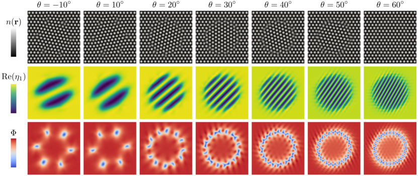
Figure 6: APFC description of (small) circular rotated inclusion in a 2D crystal with triangular symmetry (one-mode approximation), for different tilts with respect to the surrounding matrix. Different rows show: the reconstructed density $n(\mathbf{r})$, the real part of $\eta_{1}$ and $\Phi$.

An attempt to overcome this issue followed the first publications on the APFC model and consists of a polar representation of amplitudes [66]. In practice, the complex amplitudes are expressed in terms of the real fields $\phi_{m}=|\eta_{m}|$ and $\theta_{m}={\rm arg}(\eta_{m})$. The resulting set of equations for $\partial{\phi}_{m}/\partial t$ and $\partial{\theta}_{m}/\partial t$ derived from Eq. (22), have issues related to the discontinuous nature of $\theta_{m}$ and that $\phi_{m}$ vanishes in the liquid phase, in principle requiring robust and structured regularization algorithm. Therefore, further approximations are introduced [66]: i) a hybrid formulation exploiting the aforementioned polar representation only for crystal bulk, i.e. away from defects and interfaces, while solving the equations for the complex amplitudes everywhere else; ii) neglecting third and higher-order spatial derivatives of $\phi_{m}$ and $\theta_{m}$ in their dynamics and iii) assuming that gradients in the phase are zero within grains. This method has been shown to allow for efficient inhomogenous spatial discretization for numerical methods working in real space.

Recently the same issue has been addressed by exploiting a Cartesian representation of the amplitudes and allowing for local rotation of the basis vector $\mathbf{G}_{m}$ [67, 68]. This model considers a set of locally rotated amplitudes $\tilde{\eta}_{m}$ such as $\eta_{m}=\tilde{\eta}_{m}\rme^{-{\mathbb{i}}\Delta\mathbf{G}_{m}(\Theta)\cdot\mathbf{r}}$. A rotation field $\Theta$ is then computed such that $\eta_{m}$ have vanishing oscillation, i.e., satisfying the condition

$$\nabla\tilde{\eta}_{m}=(\nabla\eta_{m})\rme^{-{\mathbb{i}}\Delta\mathbf{G}_{m}(\Theta)\cdot\mathbf{r}}-{\mathbb{i}}\eta_{m}\Delta\mathbf{G}_{m}(\Theta)\rme^{-{\mathbb{i}}\Delta\mathbf{G}_{m}(\Theta)\cdot\mathbf{r}}=0,$$ (85)

thus

$$\Delta\mathbf{G}_{m}(\Theta)=\mathbf{G}_{m}(\Theta)-\mathbf{G}_{m}=\frac{\nabla\eta_{m}}{{\mathbb{i}}\eta_{m}}.$$ (86)

The local rotation field may be explicitly extracted from amplitudes, e.g. exploiting the results reported in [14]. Then, it may be shown [67, 68] that operators defined in the rotated system, $\mathcal{O}^{\Theta}$, applied to rotated fields, $f^{\Theta}$, transform as $\mathcal{O}^{\Theta}f^{\Theta}=\rme^{-{\mathbb{i}}\Delta\mathbf{G}_{m}(\Theta)\cdot\mathbf{r}}\mathcal{O}f$, as e.g. ${\partial\eta_{m}^{\Theta}}/{\partial t}=\rme^{-{\mathbb{i}}\Delta\mathbf{G}_{m}(\Theta)\cdot\mathbf{r}}{\partial\eta_{m}}/{\partial t}$ or $\mathcal{G}_{m}^{\Theta}\eta_{m}^{\Theta}=\rme^{-{\mathbb{i}}\Delta\mathbf{G}_{m}(\Theta)\cdot\mathbf{r}}\mathcal{G}_{m}\eta_{m}$. The evolution for $\eta^{\Theta}$ is evaluated while computing $\mathbf{G}_{m}(\Theta)$ everywhere. This approach still requires a proper numerical implementation [67], but has been proved successful in describing crystal structures through the “rotated” amplitudes avoiding beats due to crystal rotation, exploiting efficient mesh refinement (see Sec. 3.4), and matching the dynamics obtained by the original amplitude expansion. Importantly, this approach has also been combined with an algorithm selecting the closest reference crystal for a given local orientation [68] which avoids the presence of unphysical grain boundaries, at least in two dimensions for triangular lattices.

5.2 Elastic relaxation and mechanical equilibrium

The dynamics of the PFC model and, in turn, its amplitude expansion approximation, was initially assumed to be overdamped, i.e. driven by minimization of the corresponding free-energy functional through a gradient flow [1, 7]. Although this setting can be justified in some circumstances, it constrains the dynamic to diffusive timescales. This may lead to some issues for the description of elastic relaxation, which usually occurs on faster timescales with respect to the diffusive dynamics of the density field. A few investigations addressed these issues, delivering either a framework able to ensure mechanical equilibrium at every time, describing the limit of instantaneous elastic relaxation [75, 15, 16], or modeling explicitly elastic excitations [54].

In the work of Heinonen et al [75, 115], the amplitudes are expressed similarly to Eq. (56), assuming small displacements in $\mathbf{u}$. Then a formal separation of the timescales of the field $\phi_{m}$ from the field $\theta_{m}$, is considered. To ensure mechanical equilibrium, i.e. $\nabla\cdot\boldsymbol{\sigma}=0$, it is then demonstrated to be equivalent to solving

$$\sum_{m}^{M}\mathbf{G}_{m}\frac{d\theta_{m}}{dt}=-\sum_{m}^{M}\mathbf{G}_{m}{\rm Im}\left(\frac{1}{\eta_{m}}\frac{\delta F_{\eta}}{\delta\eta_{m}^{*}}\right)=-\frac{1}{2}\sum_{m}^{M}\mathbf{G}_{m}\frac{\delta F_{\eta}}{\delta\theta_{m}}=0,$$ (87)

at every step after solving for $\partial\eta_{m}/\partial t$. In [75], a factor $\phi_{m}^{-2}$ appears in the second-last term in (87). However, as discussed in [115], this expression allows for a more formal connection to the displacement $\mathbf{u}$. Moreover, equilibrating Eq. (87) would corresponds to a real energy minimization problem.

A different approach, which computes the mechanical equilibrium deformation from the incompatible one, fully accounting for the singular distortion of defects as conveyed by $n$ and/or $\eta_{m}$ has been proposed in Ref. [15] for PFC and then translated to APFC in Ref. [16]. Therein, the smooth distortion $u_{i}^{\delta}$ required to fulfill mechanical equilibrium is determined, and then the amplitudes are corrected as $\eta_{m}^{\rm m.e.}=\eta_{m}\rme^{-i\mathbf{G}_{m}\cdot\mathbf{u}^{\delta}}$. In brief, the smooth stress, ${\sigma}^{\delta}_{ij}$, to be added to the stress field computed from the amplitudes, $\sigma^{\eta}_{ij}$ (see also Sec. 4.2), to satisfy mechanical equilibrium is obtained through the Airy Function ($\chi$) formalism:

$$\begin{split}\sigma^{\delta}_{ij}=&\sigma^{\rm m.e.}_{ij}-\sigma^{\eta}_{ij}=\epsilon_{ik}\epsilon_{jl}\partial_{kl}\chi-\sigma_{ij}^{\eta},\\ (1-\nu)\nabla^{4}\chi=&2\mu\epsilon_{ij}\partial_{i}B_{j}(\mathbf{r})=(\epsilon_{ik}\epsilon_{jl}\partial_{ij}\sigma_{kl}^{\eta}-\nu\nabla^{2}\sigma_{kk}^{\eta}),\end{split}$$ (88)

where $\mathbf{B}(\mathbf{r})$ the Burgers vector density, and $\nu$, $\uplambda$ and $\upmu$ as in Sec. 4.4, while $\mathbf{u}^{\delta}$ is then computed exploiting a Helmholtz decomposition into curl- and divergence-free parts,

$$u_{i}^{\delta}=\partial_{i}\varphi+\epsilon_{ij}\partial_{j}\alpha,\qquad\nabla^{2}\varphi={\rm{Tr}}(\mathbf{U}^{\delta}),\qquad\nabla^{4}\alpha=-2\epsilon_{ij}\partial_{ik}U_{jk}^{\delta}.$$ (89)

Once $u_{i}^{\delta}$ is calculated, correction to the amplitudes can be imposed. This approach has been shown to work well in two dimensions for isotropic materials, while its generalization to three dimensions is non-trivial due to the Airy function formalism. A more general method to correct $n$ by computing $\mathbf{u}^{\delta}$ in three dimensions has been recently proposed in Ref [96] for PFC, and it is expected to work for the APFC model.

In Ref. [54], a model accounting explicitly for elastic relaxation has been considered by coupling the mesoscale description of the microscopic structure of the materials achieved by amplitudes to a hydrodynamic velocity field. It recovers the instantaneous relaxation as a limit of the model. It consists of describing the crystal lattice through $\eta_{m}$ and a slowly varying density field, $n_{\rm o}$, via the energy (15). The evolution laws are then derived accounting for mass density and momentum density conservation and read

$$\begin{split}n_{\rm o}\frac{D\mathbf{v}}{Dt}=&-n_{\rm o}\nabla\frac{\delta\mathcal{F}}{\delta n_{\rm o}}-\sum_{m}^{M}\left[\eta_{m}^{*}\mathcal{Q}_{m}\frac{\delta\mathcal{F}}{\delta\eta_{m}^{*}}+\text{c.c.}\right]+\mu_{\rm S}\nabla^{2}\mathbf{v}+(\mu_{\rm B}-\mu_{\rm S})\nabla(\nabla\cdot\mathbf{v}),\\ \frac{\partial n_{\rm o}}{\partial t}=&-\nabla\cdot(n_{\rm o}\mathbf{v})+\mu_{n}\nabla^{2}\frac{\delta\mathcal{F}}{\delta n_{\rm o}}+\frac{1}{2}\mu_{n}\nabla^{2}(|\mathbf{v}|^{2}),\\ \frac{\partial\eta_{m}}{\partial t}=&-\mathcal{Q}_{m}\cdot(\eta_{m}\mathbf{v})-\mu_{\eta}|\mathbf{G}_{m}|^{2}\frac{\delta\mathcal{F}}{\delta\eta_{m}^{*}},\end{split}$$ (90)

with $\mathbf{v}$ the velocity field, $D\mathbf{v}/Dt=\partial\mathbf{v}/\partial t+\mathbf{v}\cdot\nabla\mathbf{v}$, $\mathcal{Q}_{m}=\nabla+{\mathbb{i}}\mathbf{G}_{m}$, and $\mu_{\eta}$, $\mu_{n}$, $\mu_{\rm B}$, $\mu_{\rm S}$ are parameters. Previous attempts to include fast time scales in the dynamics introduced an explicit second order time derivative in the equation of motion for the PFC mass density field [116, 117]. This approach gives rise to short wavelength oscillations accelerating relaxation processes, but fails to describe large scale vibrations [55]. The model described by Eq. (90) gives the correct long wavelength elastic wave dispersion relationship $(\omega\sim k)$.

A key test case for all the approaches reported in this section is the shrinkage of rotated grains (see Fig. 7). Their results consistently show a faster dynamic in the limit of instantaneous mechanical equilibrium [75, 12, 16] while tuning of parameters in the model reported in Eq. (90) allows for the investigation of intermediate regimes [54].

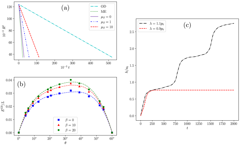
Figure 7: Representative results for extensions of the APFC model. (a) Shrinkage of a circular small-angle grain boundary (2D, triangular lattice) in terms of its radius $R(t)$ with the model illustrated in Eq. (90) (for different $\mu_{S}$), instantaneous mechanical equilibrium (ME) as from Eq. (87), and classical (overdamped) APFC dynamics (OD). Reconstructed from Ref. [54]. (b) (Symmetric) grain-boundary energy per unit length $E^{\rm GB}/L$ (2D, triangular bicrystal) as a function of the tilt angle $\theta$ for different $\beta$ values in Eq. (91). Reconstructed from Ref.  [60]. (c) Sample growth of a one dimensional front for two driving forces $\lambda$. Reconstructed from Ref. [118].

5.3 Control of interface and defect energy

The original APFC (or PFC) model contains a small set of parameters which limits quantitative fitting to match experimental measures or theoretical calculations. In Ref. [60], it has been shown that the addition of a single term to the free energy functional can be used to control the solid-liquid interface and defect energies in a well-controlled fashion, without affecting the crystal structure. Exploiting the information conveyed by $\Phi=2\sum_{m}^{M}|\eta_{m}|^{2}$, which is a measure of the crystalline order, and in analogy with the gradient term of order parameters in interfacial free energies [119], an additional energy contribution can be phenomenologically introduced in Eq. (21), reading

$$F_{\beta}=\int_{\Omega}\frac{\beta}{4}|\nabla\Phi|^{2}\text{d}\mathbf{r},$$ (91)

where $\beta$ is a free parameter. This leads to an additional term to Eq. (22) as

$$\frac{\delta F_{\beta}}{\delta\eta_{m}^{*}}=-\beta\eta_{m}\nabla^{2}\Phi.$$ (92)

For small $\beta$, this additional contribution is found to change the interface and defect energy linearly with $\beta$, while deviations are observed for large values. Fig. 7(b) shows the tuning of symmetric tilt grain boundary energies by $\beta$ due to the local change in the defect-core energies [60]. Notice that, due to the issues discussed in Sec. 5.1, it is not possible to compute the whole range of $\theta$ only by increasing the relative angle (see also [9]). In this case, energy values for theta $\gtrless 30^{\circ}$ are obtained with two different simulation settings. The framework reported in [68] would allow addressing these calculations without considering such different settings.

It is worth mentioning that formulations allowing for tunable energies at defects and interfaces similar to the one discussed here can be devised from microscopic length scales exploiting smoothing kernels in Fourier space [120, 121].

5.4 Lack of barriers

In the derivation of the amplitude equations it was implicitly assumed that the atomic- and meso-scales (interface widths, etc.) completely decouple. It appears that this approximation eliminates barriers for defect or grain boundary motion. Huang has shown that incorporating the first-order coupling of the atomic and mesoscales leads to interface pinning [118]. Consider multiplying the equation of motion by $\rme^{-{\mathbb{i}}\mathbf{q}\cdot\mathbf{r}}$ and integrating over a unit cell while keeping terms previously assumed to be zero. This leads to additional terms in Eq. (22). For instance, for a triangular lattice:

$$\begin{split}\frac{\partial\eta_{m}}{\partial t}=&\mathcal{L}_{m}\frac{\delta F_{\eta}}{\delta\eta_{m}^{*}}\approx-|\mathbf{G}_{m}|^{2}\bigg{[}A\mathcal{G}_{m}^{2}\eta_{m}+B\eta_{m}+3D(\Phi-|\eta_{m}|^{2}))\eta_{m}+\frac{\partial f^{\rm s}}{\partial\eta_{m}^{*}}\\ &+\frac{1}{A_{\rm u.c.}}\int_{\rm u.c.}\text{d}\mathbf{r}^{\,\prime}f_{p_{1}}\rme^{-{\mathbb{i}}q_{\rm o}y^{\prime}}+(\cdots)\bigg{]},\end{split}$$ (93)

where $A_{\rm u.c.}$ is the area of a unit cell and

$$f_{p_{1}}=3q_{\rm o}^{2}\left[(6n_{\rm o}+2C)\eta_{1}\eta_{2}^{*}+3v(\eta_{1}^{2}\eta_{3}+\eta_{2}^{*^{2}}\eta_{3}^{*})\right],$$ (94)

with $(\cdots)$ implying six other similar terms that contain a $\rme^{-{\mathbb{i}}\mathbf{q}\cdot\mathbf{r}^{\prime}}$ term (see reference [118] for details). The last term(s) in Eq. (93) implicitly couple atomic ($\rme^{-{\mathbb{i}}q_{0}y^{\prime}}$) and slow scales ($\eta_{m}$) terms. The equation for the average density becomes

$$\begin{split}\frac{\partial n_{\rm o}}{\partial t}=&\nabla^{2}\frac{\delta F_{\eta}}{\delta n_{\rm o}}-\frac{1}{A_{\rm u.c.}}\int_{\rm u.c.}\text{d}\mathbf{r}^{\,\prime}f^{*}_{p_{1}}\rme^{-{\mathbb{i}}q_{0}(\sqrt{3}/2x^{\prime}+3/2y^{\prime})}+(\cdots).\end{split}$$ (95)

To understand the consequences of this coupling, Huang derived an equation of motion for a liquid/solid front moving in the $y$ direction with slow variations in the $x$ direction using the projection operator method of Elder et al[5]. In this method a coordinate transformation from $(x,y)$ to $(u,s)$ is made where $u$ is a coordinate normal to the interface position and $s$ is parallel. Equation (93) (in the limit $\mathcal{L}_{m}\approx-|{\bf G}_{m}|^{2}=-1$) is multiplied by $\partial\eta_{m}/\partial u$ and Eq. (95) by $\partial n_{\rm o}/\partial u$ and integrated over $u$ in the inner region. In the outer regime the Equations (93) and (95) are linearized around a liquid state and then solved using Green’s functions. The inner and outer solutions are then matched such that the chemical potential is continuous across the interface.

One main result of these calculations is the equation for the interface normal velocity, $v_{n}$, given by

$$c_{0}v_{n}=\lambda-\gamma\kappa-p_{0}\sin(q_{0}h+\phi),$$ (96)

where $c_{0}$ is the kinetic coefficient, $\lambda\propto\Delta n_{0}^{0}\delta\mu(0,s)$, $\Delta n_{0}^{0}$ is the difference in liquid/solid density, $\delta\mu(0,s)$ is the chemical potential difference from equilibrium along the interface, $\gamma$ is the surface tension, $\kappa$ is the curvature, $p_{0}$ is the pinning strength, $h$ is the distance from the front and $\phi$ is the phase. Expressions for each of these terms is given in Huang [118]. This equation coupled with mass diffusion in the outer regions ($\eta_{m}$ at equilibrium liquid values) and the usually matching condition $v_{n}\Delta n_{0}^{0}=\partial\delta\mu/\partial u|_{0^{-}}-\partial\delta\mu/\partial u|_{0^{+}}$ constitutes a free boundary problem.

If gradients in $h$ are assumed to be small, Eq. (96) reduces to

$$c_{0}\frac{\partial h}{\partial t}=\lambda+\gamma\frac{\partial^{2}h}{\partial x^{2}}+\frac{\lambda}{2}\left(\frac{\partial h}{\partial x}\right)^{2}-p_{0}\sin(q_{0}h+\phi).$$ (97)

In the limit of non-conserved dynamics (fixed $\lambda$) this is a driven sine-Gordon equation introduced by Hwa et al[122] to study, when thermal fluctuations are included, the interface roughening during crystal growth. Huang showed that the pinning term can lead to step by step growth of the interface as is observed in experiments and even completely arresting the growth if the driving force ($\lambda$) is too small, as illustrated in Fig. 7(c). It is also shown that the pinning strength increases as temperature (controlled by $B=\Delta\texttt{B}^{0}$) or the elastic moduli (controlled by $A=\texttt{B}^{x}$) are lowered as both have the effect of decreasing the width of the liquid/solid domain wall. Later, Huang [123] extended this work to a binary system with a eutectic phase diagram and derived more general expressions for the surface energy and barrier strength as a function of concentration, temperature, and crystallographic orientation of the liquid/solid front.

6 Applications

6.1 Solid-liquid interfaces and the phase field limit

Solid-liquid interfaces are regions where $n$ may vary over length scales larger than the atomic spacing. Therefore, the APFC model may be exploited to focus on these regions while neglecting the fine details at the atomic scale elsewhere [124]. Real amplitudes have been first considered to address the modeling of solid-liquid interfaces in the seminal works by Khachaturyan [25, 26]. Therein, the order parameters resemble the ones entering classical phase-field approaches [125, 126, 127, 48] and they may be linked to atomistic descriptions. They can be used, for instance, to account for bridging-scale descriptions of elasticity effects by means of additional contributions as, e.g., in the presence of precipitates, alloys, or point defects.[128, 129, 130, 131, 132]. However, this approach does not directly encode rotational invariance and elasticity associated with the deformations of the crystal lattice.

In Refs. [45, 133, 61], traveling waves characterized by the ansatz (4) have been shown to describe the solid-liquid interfaces within PFC quite well near melting. Real amplitudes result in a classical phase-field model. Indeed, it is shown that a general form for the free energy can be obtained by considering real amplitudes,

$$F_{\phi}=\int_{\Omega}\text{d}\mathbf{r}\big{[}\texttt{a}\phi^{2}+\texttt{b}\phi^{3}+\texttt{c}\phi^{4}+\texttt{d}|\nabla\phi|^{2}\big{]},$$ (98)

where the parameters a, b, c, d depend on the lattice symmetry and the number of modes considered. Different crystalline cubic lattices, and their effect on growth dynamics are still retained [61]. In addition, the framework is consistent with atomistic simulations and can be used for matching parameters to specific materials.

In Refs. [124, 134] similar underlying ideas led to a phase-field model connecting anisotropic surface energy and corresponding Wulff shapes to the lattice symmetry of various crystals through the choice of reciprocal lattice vectors. The model remarkably encodes a regularization term leading to corner rounding of faceted shapes similarly to diffuse interface theories [135, 136, 137]. Amplitudes are assumed to be real, but they are still considered separate variables. In the notation adopted in this review from Eq. (21), and assuming zero average density, this gives

$$F_{\phi_{m}}=\int_{\Omega}\text{d}\mathbf{r}\bigg{[}\sum_{m}^{M}\bigg{(}A[\nabla^{2}\phi_{m}]^{2}+4A[\mathbf{G}_{m}\cdot\nabla\phi_{m}]^{2}-\frac{3D}{2}\phi_{m}^{4}\bigg{)}+\frac{B}{2}\Phi+\frac{3D}{4}\Phi^{2}+f^{\rm s}(\{\phi_{m}\})\bigg{]},$$ (99)

with $\Phi=2\sum_{m}^{M}\phi_{m}^{2}$ and $f^{\rm s}(\{\phi_{m}\})$ the polynomial as in Sec. 2.3 but as function of the real amplitudes only. Eq. (99) is similar to Ginzburg-Landau free energies entering multi-order-parameter phase-field models. The higher-order gradient contribution $[\nabla^{2}\phi_{m}]^{2}$ enforces the rounding of corners appearing among facets. A coefficient may be also introduced to tune its influence [134].

6.2 Grain growth with dislocation networks and small-angle grain boundaries

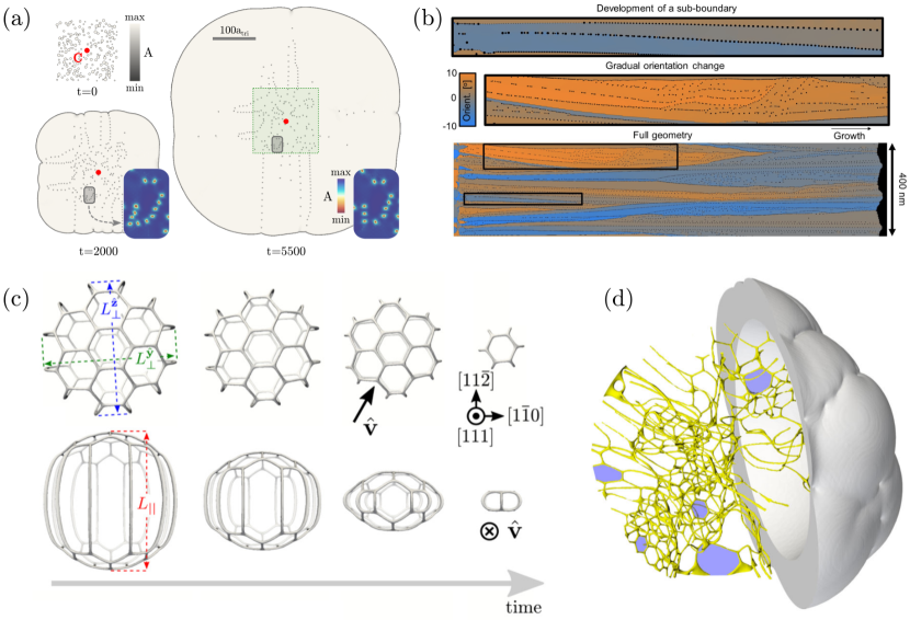
Figure 8: Examples of crystal growth and defects networks as obtained by APFC simulations. (a) Growth of $200$ seeds with orientations ranging in $(-15^{\circ},15^{\circ})$, forming straight sub-boundaries at later stages in a growing polycrystal. Reprinted from [77] $\copyright$ IOP Publishing Ltd. All rights reserved. (b) Sub-boundaries and orientational gradients in thin aluminium films by APFC. Reprinted from [76], under a creative commons attribution (CC BY) license. (c) Evolution of the defect network forming between an FCC crystal and spherical inclusion with the same structure tilted by $5^{\circ}$ about the [111] direction. Views aligned (top) and perpendicular (bottom) to the rotation axis are shown (see also the orientation of $\hat{\mathbf{v}}$). The network shrinks anisotropically with $\dot{L}_{||}>\dot{L}^{\hat{\mathbf{y}}}\sim\dot{L}^{\hat{\mathbf{x}}}$. Reprinted with permission from [138] $\copyright$ (2018) by the American Physical Society. (d) Network forming after the growth and impingement of thirty crystals with random tilt $\theta\in(-10^{\circ},10^{\circ})$ about the $[111]$ direction. Defects (yellow network) are shown within a spherical region at the center of the growing polycrystal. Adapted from [14], under a creative commons attribution (CC BY) license.

The PFC model has been exploited to investigate rather small systems due to the atomic-scale resolution. According to the features described in Sec. 4 and 5, the APFC is especially suited to describe systems with small deformation and rotation while including isolated defects such as dislocations. Examples include small-angle GBs in graphene structures [9], GBs premelting and shearing in BCC iron [139], and the dynamics of small-angle GBs in general [73]. In two dimensions, it is possible to examine systems on the micrometer scale [77, 28] (see, e.g., Fig. 8(a)). A recent, remarkable application at this length scale is the simulation of sub-boundaries formation due to orientational gradients in thin aluminium films [76, 140] (Fig. 8(b)).

The limitation in size for PFC becomes even more evident in three dimensions, requiring advanced numerical methods to simulate rather small systems [87, 10]. The APFC model has been proved powerful in addressing the study of defects in crystalline systems in three dimensions [14, 138, 77]. In particular, small-angle grain boundaries can be well captured and also characterized thanks to the advanced description of elasticity as described in Sec. 4. Representative cases are the shrinkage of dislocation networks forming at the boundaries between rotated inclusions and unrotated surrounding matrix (see Fig. 8(c)), also in combination with additional effects (see also Sec. 6.3), and the growth of slightly misoriented crystal seeds (see Fig. 8(d)). Interestingly, the shrinkage or rotated inclusions and the resulting dislocation networks have been proposed directly using a classical PFC approach [10]. This investigation delivered very similar results to the ones obtained by APFC, as reported for instance in Fig. 8(c), thus assessing the coarse-graining achieved by the APFC model in an applied case.

The shrinkage of grains is generally associated with their rotation. A fingerprint of this process emerges in APFC, as shown in Ref. [14] where rotations are tracked thanks to Eq. (69). Therein it is shown that when defects at the boundary of a grain get closer, their deformation fields superpose, increasing the effective orientation of the grain.

6.3 Binary systems

Coarse-grained approaches are often required in multiphase systems and alloys to handle simultaneously the deformation induced in the lattice, the resulting phase separations leading to Cottrell atmospheres [141, 142, 143], and effects on dislocation motion. The APFC model has been proved powerful in describing these effects at the mesoscale for binary systems, beyond results achieved by focusing on either atomistic or continuum length scales [144, 145, 146, 147, 148, 149]. Also, it can be used to study these systems comprehensively, without focusing on concentration profiles, stress distribution around dislocations, and the force-velocity curves for defect motion separately.

The original binary PFC model [24] is formulated in terms of the dimensionless atomic number density variation field and a solute concentration field $\psi$. In the APFC model, the expansion Eq. (17) is considered and a Vegard’s law for the lattice spacing $R=R_{0}(1+\alpha\psi)$ is assumed with $\alpha$ the solute expansion coefficient. This results in an energy [6, 13]

$$\begin{split}F_{\alpha\psi}=F_{\eta}+\int_{\Omega}\bigg{[}&(\texttt{w}+\texttt{Y}\Phi)\frac{\psi^{2}}{2}+\frac{\texttt{u}}{4}\psi^{4}+\frac{\texttt{K}}{2}|\nabla\psi|^{2}\\ &-2A\alpha\sum_{m}^{M}|\mathbf{G}_{m}|^{2}\left(\eta_{m}{\cal G}_{m}^{*}\eta_{m}^{*}+{\rm\text{c.c.}}\right)\psi\bigg{]}d\mathbf{r},\end{split}$$ (100)

with definitions as in previous sections and w, u, Y, K, are additional model parameters as described in Ref. [24]. Dynamics in terms of $\partial{\eta_{m}}/\partial t$ is then described by Eq. (13) with energy (100) and $\partial{\psi}/\partial t=\nabla^{2}\delta F_{\alpha\psi}/\delta\psi$, similarly to (16). It can be shown that, given $\mathbf{G}_{m}$ the basic wave vectors corresponding to a pure system, the equilibrium wave vectors for binary systems read $\mathbf{G}_{m}^{\,\rm eq}=\mathbf{G}_{m}\sqrt{1-2\alpha\psi}$ [29].

This approach allows the study of solute segregation and migration at grain boundaries, eutectic solidification, and quantum dot formation on nanomembranes [74, 6, 150, 13]. A similar approach has been exploited to accurately describe the interactions among grain boundaries and precipitates in two-phase solids [59, 69].

By applying the framework illustrated in Sec. 4.3 to this model, the velocity of dislocations including effects of the solute segregation has been also derived. By retaining only one mode of the lowest order (with $|\mathbf{G}_{m}|=1$) and using the expression for $\partial{\eta_{m}}/\partial t$ for binary systems into Eqs. (74)–(76) one gets

$$v_{i}^{d}=\frac{8\beta Ab_{j}^{d}}{|\mathbf{b}^{d}|^{2}}\epsilon_{ik}\sum_{m}^{M}|\mathbf{G}_{m}|^{2}G_{j}^{m}G_{k}^{m}\left(G_{l}^{m}G_{p}^{m}U_{lp}-|\mathbf{G}_{m}|^{2}\alpha\delta\psi\right).$$ (101)

Eq. (101) is consistent with the classical Peach-Koehler force similarly to Eq. (78). For the case of a 2D triangular lattice or a 3D BCC crystal, the velocity takes the form

$$v_{i}^{d}=M\epsilon_{ij}\left(\sigma_{jk}b_{k}^{d}-2A\phi_{0}^{2}\alpha\delta\psi b_{k}^{d}\sum_{m}^{M}G_{k}^{m}G_{j}^{m}\right),$$ (102)

with a mobility $M=2\beta/(\phi_{0}^{2}|\mathbf{b}^{d}|^{2})$. The last term in Eqs. (101)-(102) accounts for the contribution from the compositionally generated stress, as a result of the compositional strain ($\sim\alpha\psi$) arising from local concentration variations, i.e. from solute preferential segregation (Cottrell atmospheres) around defects. The stress field may be written as

$$\sigma_{ij}=8AU_{kl}\sum_{m}^{M}\phi_{m}^{2}G_{i}^{m}G_{j}^{m}G_{k}^{m}G_{l}^{m}+\frac{\partial f_{\alpha\psi}}{\partial U_{ij}}.$$ (103)

with

$$f_{\alpha\psi}=-2A\alpha\sum_{m}|\mathbf{G}_{m}|^{2}\left(\eta_{m}{\cal G}_{m}^{*}\eta_{m}^{*}+{\text{c.c.}}\right)\psi\approx 8A\alpha\psi\sum_{m}^{M}\phi_{m}^{2}|\mathbf{G}_{m}|^{2}G_{i}^{m}G_{j}^{m}\partial_{j}u_{i},$$ (104)

neglecting higher order terms in the last approximation obtained with $\eta_{m}=\phi_{m}\rme^{-{\mathbb{i}}\mathbf{G}_{m}\cdot\mathbf{u}}$ [13].

Results predicted by these equations are the deflection of dislocation glide paths, the variation of climb speed and direction, and the change or prevention of defect annihilation [13]. Simulations exploiting the FEM approach outlined in Sec. 3.3 also enable the advanced description of these effects in three dimensions, in particular for small-angle grain boundaries [13].

6.4 Multi-phase systems

Most of the APFC literature focuses on systems with a single solid phase. In a seminal work by Kubstrup et al[151], studying pinning effects between different phases, namely crystalline systems having triangular/hexagonal and square lattices, a construction has been proposed handling variable phases through a single density expansion. Extending this idea, in Ref. [58] an ansatz for the atomic density has been proposed to include more symmetries at once

$$n=n_{\rm o}+\sum_{j}^{J}\eta_{j}\rme^{{\mathbb{i}}\mathbf{G}_{j}\cdot\mathbf{r}}+\sum_{m}^{M}\chi_{m}\rme^{{\mathbb{i}}\mathbf{Q}_{m}\cdot\mathbf{r}}+\text{c.c.}$$ (105)

with $\{\eta_{j}$} and $\{\chi_{m}$} representing different set of amplitudes associated to reciprocal lattice vectors $\mathbf{G}_{j}$ and $\mathbf{Q}_{m}$, respectively. These two sets were chosen to account for the first and second modes necessary for reproducing triangular and square symmetry together, namely corresponding to $J=6$ and $M=6$ amplitudes. However, they can be arranged differently among the two sums, and, importantly, a reduced set of amplitudes can be exploited (see specific choices of $\mathbf{G}_{j}$ and $\mathbf{Q}_{m}$ in Ref. [58]). Amplitude equations would simply follow from the general equations reported in Sec. 2.3. Simulations performed with this approach, combined with the formulation illustrated in Sec. 2.4 for the excess term, showed the ability to study solidification, coarsening, peritectic growth, and the emergence of the second square phase from grain boundaries and triple junctions in a triangular polycrystalline system. See an example in Fig. 9. So far, this has been shown only for the lattice symmetry mentioned above in two dimensions. The same applies to extensions of the APFC to account for additional degrees of complexity in the crystal structure, such as for the amplitude expansion of the so-called anisotropic PFC model [124, 152].

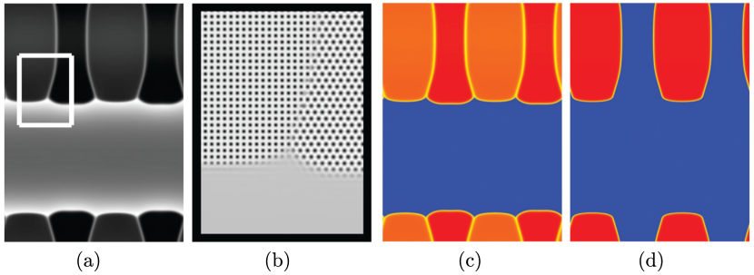
Figure 9: Example of peritectic solidification. (a) Average density $n_{\rm o}$ (white to black greyscale). (b) Reconstructed $n$ (white to black greyscale). (c) Magnitude of an amplitude $\eta$, which is nonzero in both solid structures; areas of larger magnitudes are depicted in red and zero magnitudes are blue. (d) Magnitude of amplitude $\chi$, which is only nonzero in the square phase. Color scheme is the same as in (c). Reprinted with permission from [58] $\copyright$ (2013) by the American Physical Society.

6.5 Heteroepitaxial growth

An ideal application of the APFC model is heteroepitaxial growth, where a substrate provides a single crystallographic basis for layers growing on top. In such processes, the growing film typically has similar crystal symmetry and lattice constant. The amplitudes vary on long length scales for these systems, so a relatively large computational grid spacing can be used. In this context, the large angle issue discussed in Sec. 5.1 is not present. Therefore, this would be an ideal application for using an adaptive mesh since the amplitudes in many cases vary on very large length scales. To the authors’ knowledge this has not been done to date. Nevertheless, even uniform lattices can be used to study relatively large systems.

An example application is a single or small number of mismatched layers grown on a substrate. The mismatch leads to interesting strain-induced Moiré patterns that have been observed in experimental systems [153, 154, 155]. In these cases, it is possible to model the film as a single two-dimensional layer with amplitudes. To the authors’ knowledge, the largest APFC simulation of such systems was on the study of Moiré in graphene films in which the large simulation size was $19.6$ $\mu$m $\times$ $34.0$ $\mu$m which corresponded to roughly twenty-five billion carbon atoms. Some sample works are reviewed in the next subsection. Similarly, the amplitude expansion can also effectively be used to study the growth of many layers in two and three dimensions, i.e. to examine the Asaro-Tiller-Grinfeld [156, 157, 158] instability and the subsequent nucleation of dislocations. This aspect will be also illustrated in the following. This section shows the APFC model in an applied context, reproducing experimental results and outlining general properties of mismatched, multilayered systems.

6.5.1 Ultrathin films: strain induced ordering

When a monolayer (or several layers) of one material are grown on a substrate, the lattice mismatch can lead to interesting strain induced patterns [159, 160] and the APFC model is ideally suited to model such patterns [161, 28, 162, 163, 164, 165]. Their nature depends on the misfit strain, $\varepsilon_{\rm m}=(a^{\rm s}-a^{\rm f})/a^{\rm s}$, where $a^{\rm s}$ and $a^{\rm f}$ are the substrate and film lattice constants, the relative crystal symmetry of the layer/substrate system and the film/substrate coupling strength. For example, when layers of Cu are grown on a Ru(0001) substrate, the substrate potential provides a triangular (honeycomb) array of potential maxima (minima) for the Cu atoms. Since the lattice constants of Cu and Ru(0001) are similar ($\varepsilon_{\rm m}=5.5\%$), a $1\times 1$ ordering occurs as depicted by the red dots in Fig. 10(a). For larger mismatches other orders can occur as shown in this Fig. 10 for the ordering of triangular film on a triangular substrate (TT) in (a) and a honeycomb film on a triangular substrate (HT) in (b). By symmetry a (TT) system is equivalent to a (HH) system and a (HT) system is equivalent to a (TH) system. These patterns can be characterized by two integers $(k,j)$ or equivalently a length and angle ($L,\theta$) as depicted in Fig. 10(a). The relationship between them is $L=ja^{s}_{x}(\sqrt{(2k+1)^{2}+3})/2$ and $\tan\theta=\sqrt{3}/(2k+1)$.

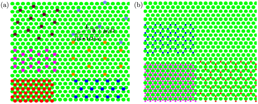
Figure 10: Ordering of a triangular (honeycomb) lattice on a substrate with a triangular array of potential maxima is depicted as green dots. In (a) the red, blue, pink, orange and purple dots correspond to $1\times 1$ (e.g., Cu/Ru(0001) or Cu/Pd(111)), $2\times 2$ (e.g., O/N(111)), $\sqrt{3}\times\sqrt{3}$ R30^∘ (e.g., Xe/graphite), $2(\sqrt{(}3)\times\sqrt{3})$, $(\sqrt{7}\times\sqrt{7})$ R19.1^∘ (e.g., S/Pd(111)) and $(\sqrt{7}\times\sqrt{7})$ R19.1^∘ respectively. In (b) the pink, red and blue atoms correspond to $1\times 1$ (e.g., graphene/Cu(111)), $2\times 2$ and $(\sqrt{3}\times\sqrt{3})$ R30^∘.

In Fig. 10(a) the $1\times 1$ state could occupy two equivalent separate sublattices, while in (b) this state has only one sublattice. In general, the degeneracy ($N_{\rm S}=$ number of equivalent sublattices) is given by,

$$N_{\rm S}=\frac{j^{2}}{2}\left(\left(2k+1\right)^{2}+3\right),$$ (106)

for the TT system and half of Eq. (106) for the HT system. Figure 11(a) illustrates the different sublattices for a TT $\sqrt{3}\times\sqrt{3}$ R30^∘ system.

The nature of the patterns that form depend on the degeneracy of sublattices, $N$, the mismatch strain, $\varepsilon_{\rm m}$, and the strength of the coupling, $V_{0}$, between the film and substrate. In the limit $V_{0}=0$, a 2D Moiré pattern forms in terms of a honeycomb array of commensurate regions bounded by a triangular network of domain walls for the TT system, with length scale $\lambda=a^{\rm f}/\varepsilon_{\rm m}$. This is illustrated in Fig. 11(b) for a $1\times 1$ system with a mismatch consistent with a Cu/Ru(0001). As $V_{0}$ increases, the commensurate regions increase in size, and the domain walls and junctions decrease in size but increase in energy. For the TT system, the displacement across a junction is larger than the displacement across a domain wall. Thus for the TT system at a certain $V_{0}$ it becomes energetically favorable to eliminate the junctions and form stripes. At even larger values of $V_{0}$ the film becomes commensurate with the substrate. A peculiar state in the TT arises for some values of $(V_{0},\varepsilon_{\rm m})$ in between the stripe and honeycomb patterns in which the junction energy is lowered by twisting the domain walls and moving the junction to a lower energy location. Sample patterns for the TT system are shown in Figs. 12(a), (b) and (c). In the case of the $1\times 1$ the junction energy is so high that it can create dislocation pairs and lead to zig-zag type patterns [165, 164].

The HT system is considerably different since the domain wall energy is higher than the junction energy and of course the symmetry is different. At very low $V_{0}$, a triangular network of commensurate regions forms. At a $V_{0}$ much higher than in the TT case, a stripe phase emerges. At a slightly larger $V_{0}$, the commensurate state appears. There appears to be no equivalent twisted state in this system. Sample stripe and triangular patterns are shown if Fig. 12(e) and (f).

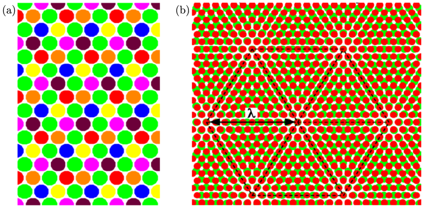
Figure 11: (a) Illustration of the six equivalent degenerate sublattices for a TT $\sqrt{3}\times\sqrt{3}$ R30^∘ system. The green dots are potential maxima due to the substrate and the other colored dots correspond to the sublattices. (b) Depiction of Moiré pattern for a $1\times 1$ system in the limit $V_{0}=0$.

To model these patterns within a PFC approach and corresponding APFC it useful to consider adding an additional coupling term, $F^{\rm c}$, to the free energy functional given in Eq. (1) of the form,

$$F^{\rm c}=\int d{\bf r}\left[Vn^{j(k+1)}\right],$$ (107)

where

$$V=V_{0}\left(\sum_{m}^{M}\rme^{{\mathbb{i}}{\bf G}^{\rm s}_{m}\cdot{\bf r}}+{\rm c.c}\right).$$ (108)

$V_{0}$ is the coupling strength, the summation is over lowest order modes needed to reconstruct the symmetry of the substrate and ${\bf G}_{m}^{\rm s}$ corresponds to the reciprocal lattice vectors of the substrate (which will have a different magnitude that the film). The coupling factor $n^{j(k+1)}$ is needed since orders greater that $1\times 1$, a coupling $Vn$ would give no contribution in the amplitude expansion, since $V$ and $n$ would have different lattice spacings. In principle, higher order harmonics of $V$ (or $n$) could be included, even though this would lead more computational expensive models. In the amplitude expansion this term leads to a coupling term $F^{\rm c}_{\eta}$, of the form

$$F^{\rm c}_{\eta}=V_{0}D_{kj}\left(\left\{\left[\left(\eta_{1}^{*}\right)^{k}\eta_{2}\right]^{j}+{\rm cyclic\ permutations}\right\}+{\rm c.c.}\right).$$ (109)

where $D_{kj}=((k+1)j)!/((kj)!j!)$. This term would be added to the free energy given in Eq. (30) for a triangular two-dimensional system. In addition, to account for the misfit strain, the operator ${\cal G}_{m}$ that enters Eq. (21) becomes

$${\cal G}_{m}\equiv\nabla^{2}+2{\mathbb{i}}{\bf G}_{m}\cdot{\bf}\nabla+1-\alpha^{2},$$ (110)

where $\alpha=1-\varepsilon_{\rm m}$.

Insight into the model can be obtained in the small deformation (${\bf u}$) limit, $\eta_{m}=\phi\rme^{-{\mathbb{i}}{\bf G}_{m}\cdot{\bf u}}$. The total free energy function reduces to a two dimensional Sine-Gordon model, i.e.,

$$\begin{split}F_{2d}^{\rm sg}=\int d{\bf r}\bigg{[}&\frac{C_{11}}{2}\big{(}(U_{xx}-\varepsilon_{\rm m})^{2}+(U_{yy}-\varepsilon_{\rm m})^{2}\big{)}+2C_{44}U_{yy}^{2}+C_{12}(U_{yy}-\varepsilon_{\rm m})(U_{xx}-\varepsilon_{\rm m})\\ &+2V_{0}D_{kj}\phi^{(k+1)j}\sum_{m}^{M}\cos({\bf G}_{m}\cdot{\bf u})\bigg{]},\end{split}$$ (111)

where $C_{11}=9A\phi^{2}$ and $C_{44}=C_{12}=3A\phi^{2}$. Unfortunately this is difficult to solve for the boundary condition of a two dimensional triangular pattern. In one dimension this reduces to a Sine-Gordon model that can be solved exactly [166]. In this model the stripe to commensurate state transition occurs when

$$\frac{P}{Ka^{2}}=\frac{\pi^{2}}{16}\varepsilon_{\rm m}^{2},$$ (112)

where $P$ is a measure of the potential between the film and substrate and $Ka^{2}$ is a measure of the elastic energy in the film. These parameters are given by

$$\frac{P}{D_{kj}\phi^{(k+1)j}V_{0}}=\left\{\begin{array}[]{cc}1/2&{\rm TT}\\ 4&{\rm TH}\end{array}\right.,$$ (113)

and

$$\frac{K}{(C_{11}+C_{12})^{2}}=\left\{\begin{array}[]{cc}(C_{11}+C_{44}/3)^{-1}&{\rm TT}\\ C_{11}^{-1}&{\rm TH}\end{array}\right..$$ (114)

Details of these calculations can be found in Elder et al[161].

The full phase diagram as a function of $\varepsilon_{\rm m}$ and the ratio of potential/elastic energy, $P/Ka^{2}$, can be obtained through numerical simulation. Sample phase diagrams are given for the $\sqrt{3}\times\sqrt{3}$ R30^∘ system for the TT and HT cases in Figs. 12(d) and (g) respectively. As can been seen in these figures for small $\varepsilon_{\rm m}$, the analytic predictions (this is true for all $(k,j)$ systems) for the stripe/commensurate transition are quite accurate and very good for the HT case for all $\varepsilon_{\rm m}$.

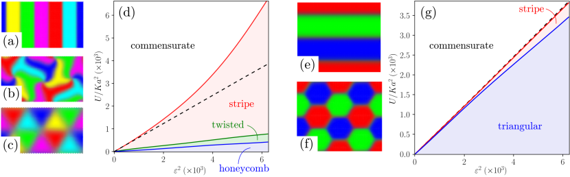
Figure 12: Sample patterns and phase diagrams for $\sqrt{3}\times\sqrt{3}$ R30^∘ system for TT (a)-(d) and HT (e)-(g) systems. For the TT system, the stripe, twisted honeycomb and honeycomb patterns are illustrated in (a), (b) and (c) respectively, and the phase diagram is shown in (d). Stripe and triangular patterns for the HT system are shown in (e) and (f) respectively and (g) shows the HT phase diagram. Each color in the patterns corresponds to a different sublattice. In (d) and (g) the dashed line is the analytic prediction for the stripe/commensurate transition given by Eq. (114). The figures were reconstructed from [161].

An interesting comparison with experiments is the Cu layers on a Ru(0001) substrate which is a $1\times 1$ TT system. In this case, varying the number of Cu layers increases the film’s elastic energy and the potential between the substrate and film. Essentially, adding more layers corresponds to reducing the ratio $P/Ka^{2}$. One layer forms a completely commensurate state, two layers form a striped state, three layers form a twisted honeycomb (or zig-zag state), and four layers form a honeycomb state. To compare with the non-equilibrium patterns observed in experiments, simulations starting from random fluctuations were conducted. The comparison of the experiments and simulations depicted in Fig. 13(a)-(c) shows a very good agreement for various patterns. In another experiment by Schmid et al[160] patterns of partially filled layers are reported. These patterns are remarkably similar to simulations of non-equilibrium patterns observed with the APFC model in the commensurate state as shown in Fig. 13(d).

Studies of the HT $1\times 1$ lead to a phase diagram similar to that shown for the $\sqrt{3}\times\sqrt{3}$ in Fig. 12. To compare with experiments, density functional theory (DFT) calculations were conducted by Smirman et al[28] to calculate the value of the dimensionless quantity $P/Ka^{2}$ for various $1\times 1$ film/substrate systems. The phase diagram accurately predicted commensurate state for twenty-five system mostly corresponding to films consisting of monolayers of InN or GaN on various substrates. In addition, the phase diagram accurately predicted a commensurate state for graphene (G) on N, and triangular patterns for G on Cu, Pd, Pt, Al, Ag, and Au. Work was also conducted to predict the wavelength of the patterns as a function of misorientation with respect to the substrate in G/Cu(111) and G/Pt(111) systems. In the absence of coupling two dimensional patterns arise with wavelength $\lambda=a^{\rm f}/\sqrt{\varepsilon_{\rm m}^{2}+2(1-\varepsilon_{\rm m})(1-\cos(\theta))}$, where $\theta$ is the misorientation angle. The study showed that as the coupling increases, the wavelength increases and interestingly the lowest energy states were not at zero degree misorientation ($0.88^{\circ}$ and $3.22^{\circ}$ for G/Cu(111) and G/Pt(111) respectively), which is unfortunately difficult to measure experimentally. However, the predicted wavelengths were consistent with the experiments of Marino et al[153] for G/Cu(111).

Other predictions of the APFC model involve the influence of defects and edges on pattern formation in the $\sqrt{3}\times\sqrt{3}$ R$30^{\circ}$ which corresponds to systems such as Xe/Pt(111) or Xe and Kr on graphite.

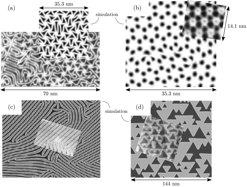
Figure 13: Comparison of simulated and experimental patterns in Cu/Ru(0001) system. The figures correspond to twisted or zig-zag, honeycomb and stripe in (a), (b) and (c) respectively. The experimental results are from Gunther et al[159]. Figure (d) compares the patterns in an experimentally partially filled layer with a simulation showing the ordering of a commensurate layer. The experimental image is taken from Schmid et al[160]. Panels (d) is reprinted with permission from [161] $\copyright$ (2017) by the American Physical Society.

6.5.2 Epitaxial growth: island formation and defect nucleation

When a material is grown epitaxially on a substrate with a mismatch strain, $\varepsilon_{\rm m}$, the film will tend to buckle and form islands or mounds as it grows due to the so-called linear Asaro-Tiller-Grinfeld (ATG) instability [156, 157, 158]. Recall that the APFC model is ideal for examining these phenomena, featuring relatively uniform amplitudes suited for adaptive meshing. In addition, it is possible to reduce the study of an ATG instability in a 2D film to a 1D problem [167, 168]. Consider expanding about the strained film such that $\eta^{\prime}_{m}=\eta_{m}\rme^{-{\mathbb{i}}\delta\mathbf{q}_{m}\cdot\mathbf{r}}$ where $\delta\mathbf{q}_{m}$ is responsible for the mismatch strain imposed by the substrate. For a triangular lattice with a strain imposed in the $x$ direction ($y$ being the growth direction) $\delta\mathbf{q}_{1}\cdot\mathbf{r}=-\delta_{x}x-\delta_{y}y/2$, $\delta\mathbf{q}_{2}\cdot\mathbf{r}=\delta_{y}y$, $\delta\mathbf{q}_{3}\cdot\mathbf{r}=\delta_{x}x-\delta_{y}y/2$, $\delta_{x}=\sqrt{3}/2\varepsilon_{\rm m}$ and $\delta_{y}$ is determined by lattice relaxation. The strained amplitudes can now be expanded about a one dimensional profile, $\eta_{j}^{0}(y)$ as follows

$$\eta_{j}^{\prime}(x,y,t)=\eta_{j}^{0}(y)+\sum_{q_{x}}\hat{\eta}_{j}(q_{x},y,t)\rme^{iq_{x}x},$$ (115)

and similarly for the average density about $n_{\rm o}^{0}(y)$

$$n_{\rm o}(x,y,t)=n_{\rm o}^{0}(y)+\sum_{q_{x}}\hat{n}_{\rm o}(q_{x},y,t)\rme^{iq_{x}x}.$$ (116)

The profiles $\eta_{j}^{0}(y)$ and $n_{\rm o}^{0}(y)$ must be determined numerically. The linearized equation of motion for the perturbed quantities $\hat{\eta}_{j}$ and $\hat{n}_{\rm o}$ are quite complex but are easily solved numerically to obtain a dispersion relation $(\omega(q_{x}))$ for the position of the liquid/solid front, i.e., the results can be fit to the form $|\hat{\eta}_{j}|$, $\hat{n}_{\rm o}\sim\rme^{\omega t}$. Dispersion relations are shown in the inset of Fig. 14(a). Various analytic studies have lead to different forms of the dispersion relation depending on what physical mechanisms are included. Surface diffusion leads to $\omega\approx\alpha_{3}q_{x}^{3}-\alpha_{4}q_{x}^{4}$ [158, 169, 170], wetting to $\omega=-\alpha_{2}q_{x}^{2}+\alpha_{3}q_{x}^{3}-\alpha_{4}q_{x}^{4}$ [171, 172], evaporation-condensation to $\omega=\alpha_{1}q_{x}-\alpha_{2}q_{x}^{2}$ [173, 174] and bulk diffusion to $\omega=\alpha_{2}q_{x}^{2}-\alpha_{3}q_{x}^{3}$ [175]. In the APFC simulations, $\omega$ can be fit to a fourth order polynomial in $q_{x}$ however none of the fits are consistent with any of the prior results. This is due to the fact that the APFC model cannot separate each of the mechanisms individually.

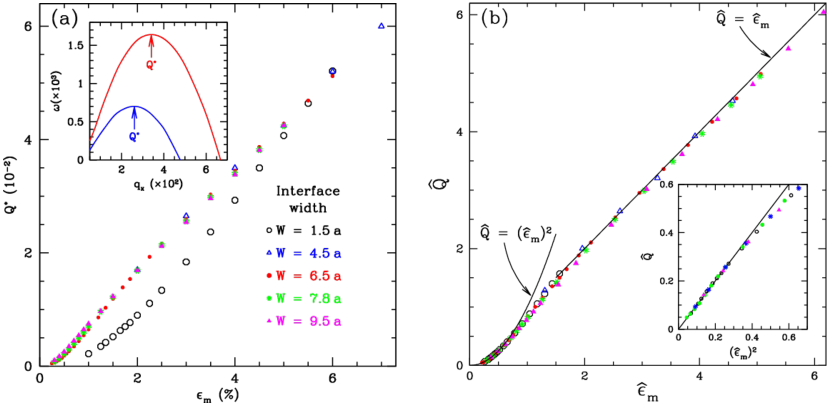
Figure 14: (a) most unstable wavevector ($Q^{*}$) is shown as a function of misfit strain ($\varepsilon_{\rm m}$) for various interface widths. In the inset dispersion relations are shown for $\varepsilon_{\rm m}=4$ % (red) and $3$ % (blue). (b) the $Q^{*}$ and $\varepsilon_{\rm m}$ are rescaled to give rise to a universal curve as described in the text. In the inset $\hat{Q}$ is shown as a function of $\hat{\varepsilon}_{\rm m}^{2}$. Details of the calculations can be found in reference [168]. Reconstructed from [167, 168].

From these studies the most unstable $q_{x}$, $Q^{*}$, can be extracted as a function of misfit strain and interface width ($W$) as shown in Fig. 14(a). The width, in the notation of Eq. (4), was altered through the variable $\texttt{B}^{x}$ since $W\sim\sqrt{\texttt{B}^{x}/|\Delta\texttt{B}^{0}|}$ [45]. For small values of $\varepsilon_{\rm m}$ it was found that $Q^{*}\sim\varepsilon_{\rm m}^{2}$ and for larger values $Q^{*}\sim\varepsilon_{\rm m}$ for all interface widths. ATG theory gives $Q^{*}\approx(E/\gamma)\varepsilon_{\rm m}^{2}$, where $E=\texttt{B}^{x}\phi^{2}/2$ is Young’s modulus, $\phi$ is the magnitude of the amplitudes in equilibrium, $\gamma$ is the surface energy which can be calculated numerically. The numerical results fit the small $\varepsilon_{\rm m}$ to $Q^{*}=4E\varepsilon_{\rm m}^{2}/3\gamma$. The linear behavior at large $\varepsilon_{\rm m}$ can be understood by considering the wavelength at which the insertion of a dislocation would lead to perfect relaxation (i.e., the addition or subtraction of a lattice point every $\lambda$ returns the lattice constant of the film to its equilibrium value). This occurs when $Q^{*}=2\pi/\lambda=q_{x}|\varepsilon_{\rm m}|$. It is interesting to note that this linear relationship was observed in experiments on SiGe/Si(001) growth [176, 177] although other explanations may exist as this is a binary system [178].

The continuum (ATG) calculation fails when the most unstable wavelength ($2\pi/Q^{*}$) becomes comparable with the interfacial thickness. If one supposes that the crossover occurs at $\varepsilon_{\rm m}^{\rm c}$ when $4E\varepsilon_{\rm m}^{\rm c}/3\gamma=q_{x}\varepsilon_{\rm m}^{\rm c}$ then $\varepsilon_{\rm m}^{\rm c}=3\gamma q_{x}/4E$ and $Q^{\rm c}=3\gamma q_{x}^{2}/4E$. Defining the scaled quantities $\hat{\varepsilon}_{\rm m}=\varepsilon_{\rm m}/\varepsilon_{\rm m}^{\rm c}$ $\hat{Q}=Q^{*}/Q^{\rm c}$ gives rise to the universal behavior shown in Fig. 14 (b). That is, the relationship between $\hat{\varepsilon}_{\rm m}$ and $\hat{Q}$ is independent of the interfacial thickness. It was found numerically that $1/Q^{\rm c}\sim\texttt{B}^{x}\sim W^{2}$.

An APFC study of the growth of islands of one material on a ribbon of another was conducted by Elder et al[6, 150]. Several experiments [179, 180, 181] had to be undertaken to examine whether the growth of islands (or quantum dots) on thin ribbons may be exploited for better control of island sizes and correlations. When an island of one material grows on an island of another material, the misfit strain will eventually lead to the nucleation of dislocation at the island/film/vapour junction. On very thin ribbons, the strain in the island can be somewhat reduced by bending the ribbons, leading the possibility of growing larger defect-free islands. An example is shown in Fig. 15. Figures (a)-(c) and (d)-(f) show the growth of an island for two different ribbon thicknesses. In (c) and (f), the final island size ($L_{f}$) at which dislocations appear indicates that $L_{f}$ is larger for the thinner ribbons. Depending on conditions it was shown in reference [150] that decreasing the ribbon size could almost double $L_{f}$. Another interesting feature emerges when the island starts to grow. It bends the ribbon such that preferential regions for island nucleation appear on the other side near the triple junctions, leading to correlated growth as shown in Fig. 15(g)-(l). This correlation could potentially be exploited to create uniform arrays of islands.

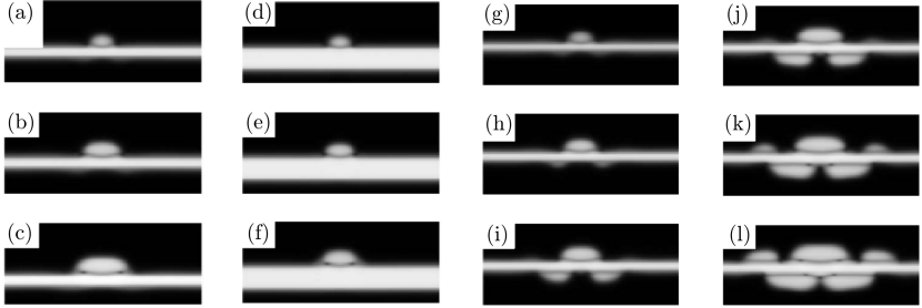
Figure 15: In this figure the magnitude of the sum of the amplitudes is shown for an island of one material grown on another. In (a)-(c) the time evolution of one island is shown. Similarly in (d)-(f) an island growth is illustrated for a thicker ribbon. In (g)-(l) the time evolution of island growth and nucleation is shown. In (a)-(f) a flux of material only came from the top, while in (g)-(l) it came from both sides of the ribbon. Reconstructed from [6].

In summary, the binary and pure APFC models provide an excellent platform for studying heteroepitaxial growth. Coupled with adaptive mesh schemes as illustrated in Sec. 3, very large simulations should be possible in both two and three dimensions.

7 Conclusions and outlook

In recent years, bridging-scale modeling has become crucial to comprehensively investigate crystalline systems, explore macroscopic effects of microscopic details, and unveil general properties and behaviors for further scale-specific characterizations. Here, an overview is provided of the model(s) obtained through the amplitude expansion of the phase-field crystal (APFC), which combines the description of crystals on relatively large (diffusive) time scales, conveyed by the PFC model [1, 7, 33], with a spatial coarse-graining. The concepts underlying its derivation have been illustrated, focusing on practical aspects such as explicit formulas, generalizations, and examples, along with presenting different formulations.

Computational aspects have also been outlined. The fields (amplitudes) to solve for within the APFC model are suited for inhomogeneous spatial discretizations, a feature that motivated its development in the first place [23]. Recently, a few optimized methods have been developed to allow for large-scale calculations and, in particular, paving the way for extensive three-dimensional calculations.

The APFC model emerges as one of a kind among mesoscale approaches: it handles the description of crystalline systems through slowly varying continuous fields, so without resolving atoms, but retains details of the crystal structure such as anisotropies and lattice defects. Namely, it merges different aspects addressed by micro- and macroscopic approaches within a single model rather than coupling models working at different time- and length scales (like other remarkable approaches as, e.g., the quasi-continuum approach [182, 183]). Among its key aspects, special attention has been given to the mesoscale description of elasticity and plasticity, being the primary goal of many coarse-grained descriptions (as the phase-field crystal itself [1, 7]). As a pivotal example, the elastic field generated by dislocations within the APFC model matches classical continuous descriptions and encodes a core regularization related to the lattice parameter. Moreover, it is expected to be affected by lattice symmetry and encodes nonlinearities. Amplitudes also allow for characterizing plasticity and defect dynamics. This description can be exploited within the broader context of PFC models as amplitudes fully characterize deformations therein [75].

Like every other model, APFC has its range of applicability, strengths, and weaknesses. One weakness is the ability to accurately predict the precise structure of atomic-scale structures such as dislocations and interfaces, similar to the drawbacks of traditional phase field models. However, it may be employed to investigate long-range effects for such systems, and extensions have been provided to improve the mesoscale descriptions with respect to the standard formulation (see, e.g., the control of energies for defects and interfaces and the modeling of Peierls barriers). Like PFC, the variational, overdamped formulation of the APFC model conveys a lack of separation among different timescales, affecting the competition among diffusion mechanisms and elastic relaxation. This issue, however, has been solved by a few different extensions, which are expected to become the standard approaches for phenomena when the separation of timescales is relevant. The most critical aspect for applications of the APFC model remains the limitation to small rotations with respect to a reference crystal orientation (see the problem of beats [66, 74, 73]). It prevents the thorough investigation of high-angle grain boundaries and polycrystalline systems. Therefore, providing a solution for this issue is a crucial challenge for achieving a general mesoscale description of crystals. To date, this aspect has been only partially addressed through a covariant formulation with respect to rotation of the crystals, which still needs to be assessed for the description of elasticity and plasticity and its compatibility with other extensions.

It is worth mentioning that in light of the limitation(s) mentioned above, the currently available APFC models should be considered valid for relatively small deformation and rotation only, de-facto for every crystalline system where defects as dislocations can be described as separated objects. However, systems featuring such conditions are common, widely studied, and exploited in several technology-relevant applications, such as single crystals, alloys, and homo-/ heteroepitaxial systems, besides small angle-grain boundaries. The overview and discussion of the main applications addressed so far in the literature illustrate this aspect.

In conclusion, this review has attempted to collect the basics and the recent developments of the APFC model. While it has been used to study several physical phenomena, its potential still has not been fully exploited. Potential applications include the investigation of three-dimensional mesoscale tracking of defects and interfaces (e.g., for heteroepitaxial systems). Moreover, besides the challenges already mentioned above, a few aspects can be identified which will improve the approach further: i) direct connections with advanced continuum theory for elasticity and plasticity, closing the gap with methods such as dislocation dynamics; ii) description of complex crystal symmetries beyond simple ones to broaden the application to technology-relevant systems; iii) extending the parametrization to include physical parameters extracted from experiments and/or other methods; iv) connections and coupling to both microscopic, fully atomistic (e.g., PFC or Molecular Dynamics) and macroscopic (e.g., phase-field, continuum elasticity) models; v) extended boundary conditions to enable investigations beyond bulk-like systems and simple geometries; vi) further development of numerical methods, keeping up with state-of-the-art numerical techniques.

References

References

- [1] Elder K R, Katakowski M, Haataja M and Grant M 2002 Phys. Rev. Lett. 88 245701
- [2] Langer J S 1980 Rev. Mod. Phys. 52 1
- [3] Karma A and Rappel W J 1996 Phys. Rev. E 53 3017
- [4] Karma A and Rappel W J 1998 Phys. Rev. E 57 4323
- [5] Elder K R, Grant M, Provatas N and Kosterlitz J M 2001 Phys. Rev. E 64 021604
- [6] Elder K R, Huang Z F and Provatas N 2010 Phys. Rev. E 81 011602
- [7] Elder K R and Grant M 2004 Phys. Rev. E 70 051605
- [8] Wu K A and Voorhees P W 2012 Acta Mater. 60 407–409
- [9] Hirvonen P, Ervasti M M, Fan Z, Jalalvand M, Seymour M, Vaez Allaei S M, Provatas N, Harju A, Elder K R and Ala-Nissila T 2016 Phys. Rev. B 94 035414
- [10] Yamanaka A, McReynolds K and Voorhees P W 2017 Acta Mater. 133 160–171
- [11] Berry J, Provatas N, Rottler J and Sinclair C W 2012 Phys. Rev. B 86 224112
- [12] Skaugen A, Angheluta L and Viñals J 2018 Phys. Rev. B 97 054113
- [13] Salvalaglio M, Voigt A, Huang Z F and Elder K R 2021 Phys. Rev. Lett. 126 185502
- [14] Salvalaglio M, Voigt A and Elder K R 2019 npj Comput. Mater. 5 48
- [15] Skaugen A, Angheluta L and Viñals J 2018 Phys. Rev. Lett. 121 255501
- [16] Salvalaglio M, Angheluta L, Huang Z f, Voigt A, Elder K R and Viñals J 2020 J. Mech. Phys. Solids 137 103856
- [17] Amodeo R J and Ghoniem N M 1990 Phys. Rev. B 41 6958
- [18] Ghoniem N M, Tong S H and Sun L Z 2000 Phys. Rev. B 61 913
- [19] Arsenlis A, Cai W, Tang M, Rhee M, Oppelstrup T, Hommes G, Pierce T G and Bulatov V V 2007 Model. Simul. Mater. Sci. Eng. 15 553
- [20] Greenwood M, Provatas N and Rottler J 2010 Phys. Rev. Lett. 105 045702
- [21] Greenwood M, Rottler J and Provatas N 2011 Phys. Rev. E 83 031601
- [22] Goldenfeld N, Athreya B P and Dantzig J A 2005 Phys. Rev. E 72 020601
- [23] Athreya B P, Nigel G and Dantzig J A 2006 Phys. Rev. E 74 011601
- [24] Elder K R, Provatas N, Berry J, Stefanovic P and Grant M 2007 Phys. Rev. B 75 064107
- [25] Khachaturyan A G 1983 The Theory of Structural Tranformation in Solids (Wiley, New York)
- [26] Khachaturyan A G 1996 Philos. Mag. A 74 3–14
- [27] Cross M C and Hohenberg P C 1993 Rev. Mod. Phys. 65 851
- [28] Smirman M, M Taha D, Singh A K, Huang Z F and Elder K R 2017 Phys. Rev. B 95 085407
- [29] Huang Z F, Elder K R and Provatas N 2010 Phys. Rev. E 82 021605
- [30] van Teeffelen S, Backofen R, Voigt A and Löwen H 2009 Phys. Rev. E 79 051404
- [31] Ramakrishnan T V and Yussouff M 1979 Phys. Rev. B 19 2775
- [32] Tupper P F and Grant M 2008 EPL (Europhysics Letters) 81 40007
- [33] Emmerich H, Löwen H, Wittkowski R, Gruhn T, Tóth G I, Tegze G and Gránásy L 2012 Adv. Phys. 61 665–743
- [34] Berry J, Provatas N, Rottler J and Sinclair C W 2014 Phys. Rev. B 89 214117
- [35] Backofen R, Barmak K, Elder K R and Voigt A 2014 Acta Mater. 64 72–77
- [36] Gránásy L, Tóth G I, Warren J A, Podmaniczky F, Tegze G, Rátkai L and Pusztai T 2019 Prog. Mater. Sci. 106 100569
- [37] Alaimo F, Praetorius S and Voigt A 2016 New J. Phys. 18 083008
- [38] Alaimo F and Voigt A 2018 Phys. Rev. E 98 032605
- [39] Huang Z F, Menzel A M and Löwen H 2020 Phys. Rev. Lett. 125 218002
- [40] Menzel A M and Löwen H 2013 Phys. Rev. Lett. 110 055702
- [41] Menzel A M, Ohta T and Löwen H 2014 Phys. Rev. E 89 022301
- [42] Praetorius S and Voigt A 2015 J. Chem. Phys. 142 154904
- [43] Aland S, Rätz A, Röger M and Voigt A 2012 Multiscale Model. Simul. 10 82–110
- [44] Ashcroft N W and Mermin N D 1976 Solid State Physics (New York: Holt, Rinehart and Winston)
- [45] Galenko P, Sanches F I and Elder K 2015 Phys. D: Nonlinear Phenom. 308 1–10
- [46] Shiwa Y 2011 Prog. Theor. Phys. 125 871–878
- [47] Oono Y and Shiwa Y 2012 Phys. Rev. E 86 061138
- [48] Provatas N and Elder K 2010 Phase-Field Methods in Materials Science and Engineering (Wiley-VCH Verlag GmbH)
- [49] Yeon D H, Huang Z F, Elder K and Thornton K 2010 Philos. Mag. 90 237–263
- [50] Hohenberg P C and Halperin B I 1977 Rev. Mod. Phys. 49 435
- [51] Grossmann B, Elder K R, Grant M and Kosterlitz J 1993 Phys. Rev. Lett. 71 3323
- [52] Drolet F, Elder K R, Grant M and Kosterlitz J 2000 Phys. Rev. E 61 6705
- [53] Elder K R, Drolet F, Grant M and Kosterlitz J 1994 Phys. Rev. Lett. 72 677
- [54] Heinonen V, Achim C V, Kosterlitz J M, Ying S C, Lowengrub J and Ala-Nissila T 2016 Phys. Rev. Lett. 116 024303
- [55] Majaniemi S and Grant M 2007 Phys. Rev. B 75 054301
- [56] Majaniemi S and Provatas N 2009 Phys. Rev. E 79 011607
- [57] Chan P Y and Goldenfeld N 2009 Phys. Rev. E 80 065105
- [58] Ofori-Opoku N, Stolle J, Huang Z F and Provatas N 2013 Phys. Rev. B 88(10) 104106
- [59] Xu Y C, Geslin P A and Karma A 2016 Phys. Rev. B 94 144106
- [60] Salvalaglio M, Backofen R, Voigt A and Elder K R 2017 Phys. Rev E 96 023301
- [61] Ankudinov V, Elder K R and Galenko P K 2020 Phys. Rev. E 102 062802
- [62] Mkhonta S K, Elder K R and Huang Z F 2013 Phys. Rev. Lett. 111 035501
- [63] Greenwood M, Ofori-Opoku N, Rottler J and Provatas N 2011 Phys. Rev. B 84 064104
- [64] Alster E, Elder K R, Hoyt J J and Voorhees P W 2017 Phys. Rev. E 95 022105
- [65] Oono Y and Puri S 1987 Phys. Rev. Lett. 58 836
- [66] Athreya B P, Goldenfeld N, Dantzig J A, Greenwood M and Provatas N 2007 Phys. Rev. E 76 056706
- [67] Berčič M and Kugler G 2018 Phys. Rev. E 98 033303
- [68] Berčič M and Kugler G 2020 Phys. Rev. E 101 043309
- [69] Geslin P a, Xu Y and Karma A 2015 Phys. Rev. Lett. 114 105501
- [70] Guan Z, Heinonen V, Lowengrub J, Wang C and Wise S M 2016 J. Comp. Phys. 321 1026
- [71] Cooley J W and Tukey J W 1965 Math. Comp. 19 297–301
- [72] Chen L Q and Shen J 1998 Comp. Phys. Comm. 108 147
- [73] Hüter C, Neugebauer J, Boussinot G, Svendsen B, Prahl U and Spatschek R 2017 Contin. Mech. Thermodyn. 29 895–911
- [74] Spatschek R and Karma A 2010 Phys. Rev. B 81 214201
- [75] Heinonen V, Achim C V, Elder K R, Buyukdagli S and Ala-Nissila T 2014 Phys. Rev. E 89 032411
- [76] Jreidini P, Pinomaa T, Wiezorek J M K, McKeown J T, Laukkanen A and Provatas N 2021 Phys. Rev. Lett. 127 205701
- [77] Praetorius S, Salvalaglio M and Voigt A 2019 Model. Simul. Mater. Sci. Eng. 27 044004
- [78] Luo X, Huang Z, Wang S, Xiao M, Meng Y, Yan H, Li Q and Wang G 2022 Electronics 11 221
- [79] Backofen R, Rätz A and Voigt A 2007 Philos. Mag. Lett. 87 813–820
- [80] Gomez H and Nogueira X 2012 Comput. Methods Appl. Mech. Eng. 249-252 52–61
- [81] Vignal P, Dalcin L, Brown D, Collier N and Calo V 2015 Comput. Struct. 158 355–368
- [82] Guo R and Xu Y 2016 SIAM J. Sci. Comput. 38 A105–A127
- [83] Wang L, Huang Y and Jiang K 2020 Numer. Math. Theor. Meth. Appl. 13 372–399
- [84] Vey S and Voigt A 2007 Comput. Visual. Sci. 10 57–67
- [85] Witkowski T, Ling S, Praetorius S and Voigt A 2015 Adv. Comput. Math. 41 1145–1177
- [86] Praetorius S and Voigt A 2015 SIAM J. Sci. Comput. 37 B425–B451
- [87] Praetorius S 2015 Efficient Solvers for the Phase-Field Crystal Equation - Development and Analysis of a Block-Preconditioner PhD Thesis Technische Universität Dresden Germany
- [88] Backofen R, Salvalaglio M and Voigt A 2022 arXiv:2202.06654
- [89] Seth B 1961 Generalized strain measure with applications to physical problems. Tech. rep. Wisconsin Univ-Madison Mathematics Research Center
- [90] Hill R 1968 J. Mech. Phys. Solids 16 229–242
- [91] Hill R 1970 Proc. R. Soc. A: Math 314 457–472
- [92] Bruhns O T 2015 The multiplicative decomposition of the deformation gradient in plasticity—origin and limitations From Creep Damage Mechanics to Homogenization Methods (Springer) pp 37–66
- [93] Neff P, Eidel B and Martin R J 2016 Arch. Ration. Mech. Anal. 222 507–572
- [94] Landau L D, Lifshitz E M, Kosevich A M and Pitaevskii L P 1986 Theory of elasticity (Elsevier)
- [95] Skogvoll V, Skaugen A and Angheluta L 2021 Phys. Rev. B 103 224107
- [96] Skogvoll V, Skaugen A, Angheluta L, Salvalaglio M and Viñals J 2021 arXiv:2110.03476
- [97] Anderson P, Hirth J and Lothe J 2017 Theory of Dislocations (Cambridge University Press)
- [98] Mazenko G F 1997 Phys. Rev. Lett. 78 401
- [99] Mazenko G F 2001 Phys. Rev. E 64 016110
- [100] Angheluta L, Jeraldo P and Goldenfeld N 2012 Phys. Rev. E 85 011153
- [101] Hüter C, Friák M, Weikamp M, Neugebauer J, Goldenfeld N, Svendsen B and Spatschek R 2016 Phys. Rev. B 93 214105
- [102] Cai W, Arsenlis A, Weinberger C and Bulatov V 2006 J. Mech. Phys. Solids 54 561–587
- [103] Head A K 1953 Proc. Roy. Soc. Lond. B 66 793–801
- [104] Marzegalli A, Brunetto M, Salvalaglio M, Montalenti F, Nicotra G, Scuderi M, Spinella C, De Seta M and Capellini G 2013 Phys. Rev. B 88 165418
- [105] Lazar M and Maugin G A 2005 Int. J. Eng. Sci. 43 1157–1184
- [106] Lazar M 2017 Philos. Mag. 97 3246–3275
- [107] Mindlin R D 1964 Arch. Ration. Mech. Anal. 16 51–78
- [108] Mindlin R and Eshel N 1968 Int. J. Solids Struct. 4 109 – 124
- [109] Lazar M and Po G 2018 J. Micromech. Mol. Phys. 03 1840008
- [110] Salvalaglio M, Chockalingam K, Voigt A and Dörfler W 2022 Examples and Counterexamples 2 100067
- [111] Kinoshita N and Mura T 1971 Phys. Status Solidi A 5 759–768
- [112] Eshelby J D 1957 Proc. Roy. Soc. Lond. A 241 376–396
- [113] Eshelby J D 1959 Proc. Roy. Soc. Lond. A 252 561–569
- [114] Mura T 1987 Micromechanics of defects in solids (Springer)
- [115] Heinonen V 2016 Phase field crystal models and fast dynamics PhD Thesis Aalto University Finland
- [116] Stefanovic P, Haataja M and Provatas N 2006 Phys. Rev. Lett. 96 225504
- [117] Galenko P, Danilov D and Lebedev V 2009 Phys. Rev. E 79 051110
- [118] Huang Z F 2013 Phys. Rev. E 87 012401
- [119] Cahn J E and Hilliard J W 1958 J. Chem. Phys. 28 258–267
- [120] Kocher G and Provatas N 2015 Phys. Rev. Lett. 114 155501
- [121] Guo C, Wang J, Wang Z, Li J, Guo Y and Huang Y 2016 Soft Matter 12 4666–4673
- [122] Hwa T, Kardar M and Paczuski M 1991 Phys. Rev. Lett. 66 441
- [123] Huang Z F 2016 Phys. Rev. E 93 022803
- [124] Kundin J, Choudhary M and Emmerich H 2014 Eur. Phys. J.: Spec. Top. 223 363–372
- [125] Chen L Q 2002 Annu. Rev. Mater. Res. 32 113–140
- [126] Boettinger W J, Warren J A, Beckermann C and Karma A 2002 Annu. Rev. Mater. Res. 32 163–194
- [127] Steinbach I 2009 Model. Simul. Mater. Sci. Eng. 17 073001
- [128] Chen L Q, Wang Y and Khachaturyan A G 1991 Phil. Mag. Lett. 64 241–251
- [129] Bugaev V N, Reichert H, Shchyglo O, Udyansky A, Sikula Y and Dosch H 2002 Phys. Rev. B 65 180203
- [130] Tewary V K 2004 Phys. Rev. B 69 094109
- [131] Varvenne C, Finel A, Le Bouar Y and Fèvre M 2012 Phys. Rev. B 86 184203
- [132] Varvenne C and Clouet E 2017 Phys. Rev. B 96 224103
- [133] Nizovtseva I G and Galenko P K 2018 Philos. Trans. R. Soc. A 376 20170202
- [134] Ofori-Opoku N, Warren J A and Voorhees P W 2018 Phys. Rev. Materials 2 083404
- [135] Wheeler A 2006 Proc. Roy. Soc. Lond. A 462 3363–3384
- [136] Torabi S, Lowengrub J, Voigt A and Wise S 2009 Proc. Roy. Soc. Lond. A 465 1337–1359
- [137] Salvalaglio M, Backofen R, Bergamaschini R, Montalenti F and Voigt A 2015 Cryst Growth Des. 15 2787–2794
- [138] Salvalaglio M, Backofen R, Elder K R and Voigt A 2018 Phys. Rev. Materials 2 053804
- [139] Adland A, Karma A, Spatschek R, Buta D and Asta M 2013 Phys. Rev. B 87 024110
- [140] Pinomaa T, Lindroos M, Jreidini P, Haapalehto M, Ammar K, Wang L, Forest S, Provatas N and Laukkanen A 2022 Phil. Trans. R. Soc. A 380 20200319
- [141] Cottrell A H, Jaswon M A and Mott N F 1949 Proc. Roy. Soc. Lond. A 199 104–114
- [142] Cottrell A H and Bilby B A 1949 Proc. Roy. Soc. Lond. A 62 49–62
- [143] Cottrell A H 1953 Dislocations and plastic flow in crystals Internat. Ser. Mono. Phys. (Oxford: Clarendon Press)
- [144] Zhang F and Curtin W A 2008 Model. Simul. Mater. Sci. Eng. 16 055006
- [145] Sills R B and Cai W 2016 Philos. Mag. 96 895–921
- [146] Gu Y and El-Awady J A 2020 Mater. Theory 4 1
- [147] Mishin Y 2019 Acta Mater. 179 383 – 395
- [148] Koju R K and Mishin Y 2020 Acta Mater. 198 111–120
- [149] Darvishi Kamachali R, Kwiatkowski da Silva A, McEniry E, Ponge D, Gault B, Neugebauer J and Raabe D 2020 npj Comput. Mater. 6 191
- [150] Elder K R and Huang Z F 2010 J. Condens. Matter Phys. 22 364103
- [151] Kubstrup C, Herrero H and Pérez-García C 1996 Phys. Rev. E 54 1560
- [152] Kundin J and Choudhary M A 2017 Model. Simul. Mater. Sci. Eng. 25 055004
- [153] Merino P, Svec M, Pinardi A L, Otero G and Martin-Gago J A 2011 ACS Nano 5 5627–5634
- [154] Roos M, Uhl B, Künzel D, Hoster H E, GroßA and Behm R J 2011 Beilstein J. Nanotechnol. 2 365–373
- [155] Balog R, Jørgensen B, Nilsson L, Andersen M, Rienks E, Bianchi M, Fanette M, Lægsgaard E, Baraldi A, Lizzit S, Sljivancanin Z, Besenbacher F, Hammer B, Pedersen T G, Hofmann P and Hornekær 2010 Nat. Mat. 9 315–319
- [156] Asaro R J and Tiller W A 1972 Metall. Trans. 3 1789–1796
- [157] Grinfeld M 1993 J. Nonlinear Sci. 31 35–83
- [158] Srolovitz D J 1989 Acta Metall. 37 621–625
- [159] Gunther C, Vrijmoeth J, Hwang R Q and Behm R J 1995 Phys. Rev. Lett. 74 754
- [160] Schmid A K, Bartelt N C, Hamilton J C, Carter C B and Hwang R Q 1997 Phys. Rev. Lett. 78 3507–3510
- [161] Elder K R, Achim C V, Granato E, Ying S C and Ala-Nissila T 2017 Phys. Rev. B 96 195439
- [162] Elder K R, Achim C V, Granato E, Ying S C and Ala-Nissila T 2016 EPL 116 56002
- [163] Elder K R, Chen Z, Elder K L M, Hirvonen P, Mkhonta S K, Ying S C, Granato E, Huang Z F and Ala Nissila T 2016 J. Chem. Phys. 144 174703
- [164] Elder K R, Rossi G, Kanerva P, Sanches F, Ying S C, Granato E, Achim C V and Ala-Nissila T 2013 Phys. Rev. B. 88 075423
- [165] Elder K R, Rossi G, Kanerva P, Sanches F, Ying S C, Granato E, Achim C V and Ala-Nissila T 2012 Phys. Rev. Lett. 108 226102
- [166] Chaikin P M and Lubensky T C 1995 Principles of Condensed Matter Physics (Cambridge University Press)
- [167] Huang Z F and Elder K R 2008 Phys. Rev. Lett. 101 158701
- [168] Huang Z F and Elder K R 2010 Phys. Rev. B 81 165421
- [169] Spencer B J, Voorhees P W and Davis S H 1991 Phys. Rev. Lett. 67 3696
- [170] Spencer B J, Voorhees P W and Davis S H 1993 J. Appl. Phys. 73 4955
- [171] Levine M S, Golovin A A, Davis S H and Voorhees P W 2007 Phys. Rev. B 75 205312
- [172] Eisenberg H R and Kandel D 2000 Phys. Rev. Lett. 85 1286
- [173] Müller J M and Grant M 1999 Phys. Rev. Lett. 82 1736
- [174] Kassner K, Misbah C, Müller J, Kappey J and Kohlert P 2001 Phys. Rev. E 63 036117
- [175] Wu K A W and Voorhees P W 2009 Phys. Rev. B 80 125408
- [176] Sutter P and Lagally M G 2000 Phys. Rev. Lett. 84 4637
- [177] Tromp R M, Ross F M and Reuter M C 2000 Phys. Rev. Lett. 84 4641
- [178] Bergamaschini R, Salvalaglio M, Backofen R, Voigt A and Montalenti F 2016 Adv. Phys. X 1 331–367
- [179] Huang M, Rugheimer P, Lagally M G and Liu F 2005 Phys. Rev. B 72 085450
- [180] Kim-Lee H J, Savage D E, Ritz C S, Lagally M G and Turner K T 2009 Phys. Rev. Lett. 102 226103
- [181] Huang M H, Ritz C S, Novakovic B, Yu D, Zhang Y, Flack F, Savage D E, Evans P G, Knezevic I, Liu F and Lagally M G 2009 ACS Nano 3 721–727
- [182] Shenoy V, Miller R, Tadmor E, Rodney D, Phillips R and Ortiz M 1999 J. Mech. Phys. Solids 47 611–642
- [183] Curtin W A and Miller R E 2003 Model. Simul. Mater. Sci. Eng. 11 R33–R68