FMP: Toward Fair Graph Message Passing against Topology Bias

Abstract

Despite recent advances in achieving fair representations and predictions through regularization, adversarial debiasing, and contrastive learning in graph neural networks (GNNs), the working mechanism (i.e., message passing) behind GNNs inducing unfairness issue remains unknown. In this work, we theoretically and experimentally demonstrate that representative aggregation in message passing schemes accumulates bias in node representation due to topology bias induced by graph topology. Thus, a Fair Message Passing (FMP) scheme is proposed to aggregate useful information from neighbors but minimize the effect of topology bias in a unified framework considering graph smoothness and fairness objectives. The proposed FMP is effective, transparent, and compatible with back-propagation training. An acceleration approach on gradient calculation is also adopted to improve algorithm efficiency. Experiments on node classification tasks demonstrate that the proposed FMP outperforms the state-of-the-art baselines in effectively and efficiently mitigating bias on three real-world datasets.

1 Introduction

Graph neural networks (GNNs) (Kipf & Welling, 2017; Veličković et al., 2018; Wu et al., 2019) are widely adopted in various domains, such as social media mining (Hamilton et al., 2017), knowledge graph (Hamaguchi et al., 2017) and recommender system (Ying et al., 2018), due to remarkable performance in learning representations. Graph learning, a topic with growing popularity, aims to learn node representation containing both topological and attribute information in a given graph. Despite the outstanding performance in various tasks, GNNs still inherit or even amplify societal bias from input graph data (Dai & Wang, 2021). The biased node representation largely limits the application of GNNs in many high-stake tasks, such as job hunting (Mehrabi et al., 2021) and crime ratio prediction (Suresh & Guttag, 2019). Hence, bias mitigation that facilitates the research on fair GNNs is in an urgent need.

In many graphs, nodes with the same sensitive attribute (e.g., ages) are more likely to get connected. For example, young people mainly make friends with people at similar ages (Dong et al., 2016). We call this phenomenon “topology bias”. Since, for each node, the node representations is learned by aggregating the representation of its neighbors in GNNs, nodes with the same sensitive attribute will be more similar after the aggregation. Specifically, we visualize the topology bias for three real-world datasets (Pokec-n, Pokec-z, and NBA) in Figure 1, where different edge types are highlighted with different colors for top-$3$ largest connected components in original graphs. Such topology bias leads to more similar node representation for those nodes with the same sensitive attribute, which is a major source for the graph representation bias.

Many existing works achieving fair node representation either rely on regularization, adversarial debiasing, or contrastive learning. These methods, however, adopt sensitive attribute information in training loss refinement, ignoring the uniqueness part (i.e., message passing) of GNNs on exploring fairness. The effect of message passing on improving fairness by eliminating topology bias is underexplored in prior works. A natural question is raised: Can message passing in GNNs aggregate useful information from neighbors and fundamentally mitigate representation bias inherited from topology bias?

In this work, we provide a positive answer via designing an effective, efficient, and transparent scheme for GNNs, called fair message passing (FMP). First, we theoretically prove that the aggregation in message passing inevitably accumulates representation bias when large topology bias exists. Second, motivated by our theoretical analysis, we plug the sensitive attribute information into the message passing scheme. Specifically, we formulate an optimization problem that integrates fairness and prediction performance objectives. Then we derive FMP to solve the problem via Fenchel conjugate and gradient descent to generate fair-and-predictive representation. Further, we demonstrate the superiority of FMP by examining its effectiveness and efficiency, where we adopt the property of softmax function to accelerate the gradient calculation over primal variables. In short, the contributions can be summarized as follows:

• To the best of our knowledge, it is the first paper to theoretically investigate how GCN-like message passing scheme amplifies representation bias according to topology bias.

• Integrated in a unified optimization framework, we develop the FMP scheme to simultaneously guarantee graph smoothness and enhance fairness, which lays a foundation for intrinsic methods on exploring fair GNNs. An acceleration method is proposed to reduce gradient computational complexity with theoretical and empirical validation.

• The effectiveness and efficiency of FMP are experimentally evaluated on three real-world datasets. The results show that compared to the state-of-the-art, our FMP exhibits a superior trade-off between prediction performance and fairness with negligibly computation overhead.

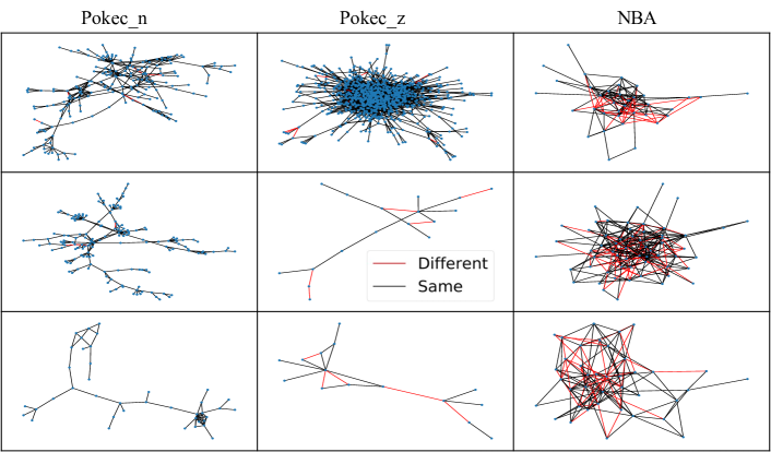
Figure 1: Visualization of topology bias in three real-world datasets, where black edges and red edges represent the edge with the same or different sensitive attributes for the connected node pair, respectively. We visualize the largest three connected components for each dataset. It is obvious that the sensitive homophily coefficients (the ratio of homo edges) are high in practice, i.e., $95.30\%$, $95.06\%$ and $72.37\%$ for Pokec-n, Pokec-z and NBA dataset, respectively.

2 Preliminaries

We adopt bold upper-case letters to denote matrix such as $\mathbf{X}$, bold lower-case letters such as $\mathbf{x}$ to denote vectors, calligraphic font such as $\mathcal{X}$ to denote set. Given a matrix $\mathbf{X}\in\mathbb{R}^{n\times d}$, the $i$-th row and $j$-th column are denoted as $\mathbf{X}_{i}$ and $\mathbf{X}_{\cdot,j}$, and the element in $i$-th row and $j$-th column is $\mathbf{X}_{i,j}$. We use the Frobenius norm, $l_{1}$ norm of matrix $\mathbf{X}$ as $||\mathbf{X}||_{F}=\sqrt{\sum_{i,j}\mathbf{X}_{i,j}^{2}}$ and $||\mathbf{X}||_{1}=\sum_{ij}|\mathbf{X}_{ij}|$, respectively. Given two matrices $\mathbf{X},\mathbf{Y}\in\mathbb{R}^{n\times d}$, the inner product is defined as $\langle\mathbf{X},\mathbf{Y}\rangle=tr(\mathbf{X}^{\top}\mathbf{Y})$, where $tr(\cdot)$ is the trace of a square matrix. $SF(\mathbf{X})$ represents softmax function with a default normalized column dimension.

Let $\mathcal{G}=\{\mathcal{V},\mathcal{E}\}$ be a graph with the node set $\mathcal{V}=\{v_{1},\cdots,v_{n}\}$ and the undirected edge set $\mathcal{E}=\{e_{1},\cdots,e_{m}\}$, where $n,m$ represent the number of node and edge, respectively. The graph structure $\mathcal{G}$ can be represented as an adjacent matrix $\mathbf{A}\in\mathbb{R}^{n\times n}$, where $\mathbf{A}_{ij}=1$ if existing edge between node $v_{i}$ and node $v_{j}$. $\mathcal{N}(i)$ denotes the neighbors of node $v_{i}$ and $\tilde{\mathcal{N}}(i)=\mathcal{N}(i)\cup\{v_{i}\}$ denotes the self-inclusive neighbors. Suppose that each node is associated with a $d$-dimensional feature vector and a (binary) sensitive attribute, the feature for all nodes and sensitive attribute are denoted as $\mathbf{X}_{ori}=\mathbb{R}^{n\times d}$ and $\mathbf{s}\in\{-1,1\}^{n}$. Define the sensitive attribute incident vector as $\Delta_{\mathbf{s}}=\frac{\mathbbm{1}_{>0}(\mathbf{s})}{||\mathbbm{1}_{>0}(\mathbf{s})||_{1}}-\frac{\mathbbm{1}_{>0}(-\mathbf{s})}{||\mathbbm{1}_{>0}(-\mathbf{s})||_{1}}$ to normalize each sensitive attribute group, where $\mathbbm{1}_{>0}(\mathbf{s})$ is an element-wise indicator function.

2.1 GNNs as Graph Signal Denoising

A GNN model is usually composed of several stacking GNN layers. Given a graph $\mathcal{G}$ with $N$ nodes, a GNN layer typically contains feature transformation $\mathbf{X}_{trans}=f_{trans}(\mathbf{X}_{ori})$ and aggregation $\mathbf{X}_{agg}=f_{agg}(\mathbf{X}_{trans}|\mathcal{G})$, where $\mathbf{X}_{ori}\in\mathbb{R}^{n\times d_{in}}$, $\mathbf{X}_{trans},\mathbf{X}_{agg}\in\mathbb{R}^{n\times d_{out}}$ represent the input and output features. The feature transformation operation transforms the node feature dimension via neural networks, and feature aggregation, updates node features based on neighbors’ features and graph topology.

Recent works (Ma et al., 2021c; Zhu et al., 2021) have established the connections between many feature aggregation operations in representative GNNs and a graph signal denoising problem with Laplacian regularization. Here, we only introduce GCN/SGC as an examples to show the connection from a perspective of graph signal denoising. The more discussions are elaborated in Appendix I. Feature aggregation in Graph Convolutional Network (GCN) or Simplifying Graph Convolutional Network (SGC) is given by $\mathbf{X}_{agg}=\tilde{\mathbf{A}}\mathbf{X}_{trans}$, where $\tilde{\mathbf{A}}=\tilde{\mathbf{D}}^{-\frac{1}{2}}\hat{\mathbf{A}}\tilde{\mathbf{D}}^{-\frac{1}{2}}$ is a normalized self-loop adjacency matrix $\hat{\mathbf{A}}=\mathbf{A}+\mathbf{I}$, and $\tilde{\mathbf{D}}$ is degree matrix of $\tilde{\mathbf{A}}$. Recent works (Ma et al., 2021c; Zhu et al., 2021) provably demonstrate that such feature aggregation is equivalent to one-step gradient descent to minimize $tr(\mathbf{F}^{\top}\big{(}\mathbf{I}-\tilde{\mathbf{A}})\mathbf{F}\big{)}$ with initialization $\mathbf{F}=\mathbf{X}_{trans}$.

2.2 Label and Sensitive Homophily in Graphs

The behaviors of graph neural networks have been investigated in the context of label homophily for connected node pairs in graphs (Ma et al., 2021b). Label homophily in graphs is typically defined to characterize the similarity of connected node labels in graphs. Here, similar node pair means that the connected nodes share the same label. From the perspective of fairness, we also define the sensitive homophily coefficient to represent the sensitive attribute similarity among connected node pairs. Informally, the coefficient for label homophily and sensitive homophily are defined as the fraction of the edges connecting the nodes of the same class label and sensitive attributes in a graph (Zhu et al., 2020; Ma et al., 2021b). We also provide the formal definition as follows:

Definition 1 (Label and Sensitive Homophily Coefficient).

Given a graph $\mathcal{G}=\{\mathcal{V},\mathcal{E}\}$ with node label vector $\mathbf{y}$, node sensitive attribute vector $\mathbf{s}$, the label and sensitive attribute homophily coefficients are defined as the fraction of edges that connect nodes with the same labels or sensitive attributes $\epsilon_{label}(\mathcal{G},\mathbf{y})=\frac{1}{|\mathcal{E}|}\sum_{(i,j)\in\mathcal{E}}\mathbbm{1}(\mathbf{y}_{i}=\mathbf{y}_{j})$, and $\epsilon_{sens}(\mathcal{G},\mathbf{s})=\frac{1}{|\mathcal{E}|}\sum_{(i,j)\in\mathcal{E}}\mathbbm{1}(\mathbf{s}_{i}=\mathbf{s}_{j})$, where $|\mathcal{E}|$ is the number of edges and $\mathbbm{1}(\cdot)$ is the indicator function.

Recent works (Ma et al., 2021b; Chien et al., 2021; Zhu et al., 2020) aim to understand the relation between the message passing in GNNs and label homophily from the interactions between GNNs (model) and graph topology (data). For graph data with a high label homophily coefficient, existing works (Ma et al., 2021b; Tang et al., 2020) have demonstrated, either provably or empirically, that the nodes with higher node degree obtain more prediction benefits in GCN, compared to the benefits that peripheral nodes obtain. As for graph data with a low label homophily coefficient, GNNs does not necessarily lead to better prediction performance compared with MLP since since the node features of neighbors with different labels contaminates the node features during feature aggregation. However, although work (Dai & Wang, 2021) empirically points out that graph data with large sensitive homophily coefficient may enhance bias inGNNs, the fundamental understanding for message passing and sensitive homophily coefficient is still missing. We provide the theoretical analysis in Section 3.

3 Graph Topology Enhances Bias in GNNs

For each node, GNNs aggregate its neighbors’ features to learn its representation. In real-world datasets, we observe a high sensitive homophily coefficient (which is even higher than the label homophily coefficient). However, existing message passing schemes tend to aggregate the node features from their neighbors with the same sensitive attributes. Thus, the common belief is that the message passing renders node representations with the same sensitive attribute more similar. However, this common belief is heuristic and the quantifiable relationship between the topology bias and representation bias is still missing. In this section, (1) we rectify such common belief and quantitatively reveal that only sufficient high sensitive homophily coefficient would lead to bias enhancement; (2) we analyze the influence of other graphs statistical information, such as the number of nodes $n$, the edge density $\rho_{d}$, and sensitive group ratio $c$, in term of bias enhancement.

Throughout our analysis, we mainly focus on $4$ characteristics of graph topology: the number of nodes $n$, the edge density $\rho_{d}$, sensitive homophily coefficient $\epsilon_{sens}$, and sensitive group ratio $c$. Specifically, we consider the synthetic random graph generation as follows:

Definition 2 ($(n,\rho_{d},\epsilon_{sens},c)$-graph).

The synthetic random graph $\mathcal{G}$ sampled from $(n,\rho_{d},\epsilon_{sens},c)$-graph satisfies the following properties: 1) the graph node number is $n$; 2) the adjacency matrix $\mathbf{A}$ satisfies $\mathbf{A}_{ij}\in\{0,1\}$ and $\mathbb{E}_{ij}[\mathbb{P}(\mathbf{A}_{ij}=1)]=\rho_{d}$; 3) given connected node pair $\mathbf{A}_{ij}=1$, the probability of connected nodes with the same sensitive attribute satisfies $\mathbb{P}(\mathbf{s}_{i}=\mathbf{s}_{j}|\mathbf{A}_{ij}=1)=\epsilon_{sens}$; 4) the binary sensitive attribute $\mathbf{s}_{i}\in\{-1,1\}$ satisfies $\mathbb{E}_{i}[\mathbb{P}(\mathbf{s}_{i}=1)]=c$; 5) independent edge generation.

We assume that node attributes in synthetic graph follow Gaussian Mixture Model $GMM(c,\mathbf{\mu}_{1},\mathbf{\Sigma}_{1},\mathbf{\mu}_{2},\mathbf{\Sigma}_{2})$. For node with sensitive attribute $\mathbf{s_{i}}=-1$ ($\mathbf{s_{i}}=1$), the node attributes $\mathbf{X}_{i}$ follows Gaussian distribution $P_{1}=\mathcal{N}(\mathbf{\mu}_{1},\mathbf{\Sigma}_{1})$ ($P_{2}=\mathcal{N}(\mathbf{\mu}_{2},\mathbf{\Sigma}_{2})$), where the node attributes with the same sensitive attribute are independent and identically distributed, and $\mathbf{\mu}_{i},\mathbf{\Sigma}_{i}$ ($i=1,2$) represent the mean vector and covariance matrix.

To measure the node representations bias, we adopt the mutual information between sensitive attribute and node attributes $I(\mathbf{s},\mathbf{X})$. Note that the exact mutual information $I(\mathbf{s},\mathbf{X})$ is intractable to estimate, an upper bound on the exact mutual information is developed as a surrogate metric in the following Theorem 1:

Theorem 1.

Suppose the synthetic graph node attribute $\mathbf{X}$ is generated based on Gaussian Mixture Model $GMM(c,\mathbf{\mu}_{1},\mathbf{\Sigma}_{1},\mathbf{\mu}_{2},\mathbf{\Sigma}_{2})$, i.e., the probability density function of node attributes for the nodes of different sensitive attribute $\mathbf{s}=\{-1,1\}$ follows $f_{\mathbf{X}}(\mathbf{X}_{i}=\mathbf{x}|\mathbf{s}_{i}=-1)\sim\mathcal{N}(\mathbf{\mu}_{1},\mathbf{\Sigma}_{1})\stackrel{{\scriptstyle\triangle}}{{=}}P_{1}$ and $f_{\mathbf{X}}(\mathbf{X}_{i}=\mathbf{x}|\mathbf{s}_{i}=1)\sim\mathcal{N}(\mathbf{\mu}_{2},\mathbf{\Sigma}_{2})\stackrel{{\scriptstyle\triangle}}{{=}}P_{2}$, and the sensitive attribute ratio satisfies $\mathbb{E}_{i}[\mathbb{P}(\mathbf{s}_{i}=1)]=c$, then the mutual information between sensitive attribute and node attributes $I(\mathbf{s},\mathbf{X})$ satisfies

$$I(\mathbf{s},\mathbf{X})\leq-(1-c)\ln\Big{[}(1-c)+c\exp\big{(}-D_{KL}(P_{1}||P_{2})\big{)}\Big{]}$$

$$-c\ln\Big{[}c+(1-c)\exp\big{(}-D_{KL}(P_{2}||P_{1})\big{)}\Big{]}\stackrel{{\scriptstyle\triangle}}{{=}}Bias(\mathbf{s},\mathbf{X}).$$

Based on Theorem 1, we can observe that lower distribution distance $D_{KL}(P_{1}||P_{2})$ or $D_{KL}(P_{2}||P_{1})$ is beneficial for reducing $Bias(\mathbf{s},\mathbf{X})$ and $I(\mathbf{s},\mathbf{X})$ since the sensitive attribute is less distinguishable based on node representations.

We focus on the role of message passing in terms of fairness. Suppose the graph adjacency matrix $\mathbf{A}$ is sampled for $(n,\rho_{d},\epsilon_{sens},c)$-graph and we adopt the GCN-like message passing $\tilde{\mathbf{X}}=\tilde{\mathbf{A}}\mathbf{X}$, where $\tilde{\mathbf{A}}$ is normalized adjacency matrix with self-loop. We define the bias difference for such message passing as $\Delta Bias=Bias(\mathbf{s},\tilde{\mathbf{X}})-Bias(\mathbf{s},\mathbf{X})$ to measure the role of graph topology. Subsequently, we provide a sufficient condition to specify the case that graph topology enhances bias in Theorem 2.

Theorem 2.

Suppose the synthetic graph node attribute $\mathbf{X}$ is generated based on Gaussian Mixture Model $GMM(c,\mathbf{\mu}_{1},\mathbf{\Sigma},\mathbf{\mu}_{2},\mathbf{\Sigma})$, and the graph adjacency matrix $\mathbf{A}$ is generated from $(n,\rho_{d},\epsilon_{sens},c)$-graph. If adopting GCN-like message passing $\tilde{\mathbf{X}}=\tilde{\mathbf{A}}\mathbf{X}$, bias will be enhanced, i.e., $\Delta Bias>0$ if the bias-enhance condition holds: $(\nu_{1}-\nu_{2})^{2}\min\{\zeta_{1},\zeta_{2}\}>1$, where $\nu_{1}-\nu_{2}<1$ represents the reduction coefficient of the distance between the mean node attributes of the two sensitive attribute group, $\zeta_{1},\zeta_{2}$ mean the connection degree of two sensitive group; the mathematical formulation is given by

$$\nu_{1}=\frac{(n_{1}-1)p_{conn}+1}{\zeta_{0}},\quad\nu_{2}=\frac{(n_{1}-1)q_{conn}}{\zeta_{1}}$$

$$\zeta_{1}=n_{-1}q_{conn}+(n_{1}-1)p_{conn}+1,$$

$$\zeta_{2}=n_{-1}p_{conn}+(n_{1}-1)q_{conn}+1$$ (1)

where the node number with the same sensitive attribute $n_{-1}=n(1-c)$, $n_{1}=nc$, intra-connect probability $p_{conn}=\mathbb{E}_{ij}[\mathbb{P}(\mathbf{A}_{ij}|\mathbf{s}_{i}=\mathbf{s}_{j})]$, and inter-connect probability $q_{conn}=\mathbb{E}_{ij}[\mathbb{P}(\mathbf{A}_{ij}|\mathbf{s}_{i}\mathbf{s}_{j}=-1)]$.

Based on Theorem 2, we have the following theoretical observations (See more elaboration in Appendix E):

• Node representation bias is enhanced by message passing for sufficient large sensitive homophily $\epsilon_{sens}$. When $\epsilon_{sens}$ approaches $1$, the inter-connect probability is $0$. Hence the mean reduction coefficient is $\nu_{1}-\nu_{2}=1$ and connection degree $\min\{\zeta_{1},\zeta_{2}\}>1$.

• The bias enhancement implicitly depends on node representation geometric differentiation, including the distance between the mean node representation within the same sensitive attribute and the scale covariance matrix. Theorem 1 implies that low mean representation distance and concentrated representation (low covariance matrix) leads to fair representation. However, GCN-like message passing renders the mean node representation distance reduction $\nu_{1}-\nu_{2}$ and concentrated for each sensitive attribute group, which is an “adversarial” effect for fairness and the mean distance and covariance reduction is controlled by sensitive homophily coefficient.

• The bias is enlarged as node number $n$ being increased. For large node number $n$, the mean distance almost keeps constant since $\nu_{1}\approx\frac{cp_{conn}}{(1-c)q_{conn}+cp_{conn}}$, $\nu_{2}\approx\frac{cq_{conn}}{(1-c)p_{conn}+cq_{conn}}$, and $\zeta_{1},\zeta_{2}$ are almost proportional to node number $n$. Therefore, the bias-enhancement condition can be more easily satisfied in large graphs.

• The bias is enlarged as graph connection density $\rho$ being increased. Based on Appendix C, inter-connect and intra-connect probability is proportional to graph connection density $\rho_{d}$, and the mean distance almostly keeps constant and $\zeta_{1},\zeta_{2}$ are almost proportional to $\rho_{d}$. Therefore, the bias-enhancement condition can be more easily satisfied in dense graphs.

• When the sensitive attribute is more balanced (i.e.,) the bias will be enlarged. The difference of intra-connected probability $p_{conn}$ and inter-connected probability $q_{conn}$ is increased if the sensitive attribute is highly balanced. Therefore, the aggregated node representation will adopt more neighbor’s information with the same sensitive attribute during message passing and amplify representation bias.

4 Fair Message Passing

Section 3 demonstrates that GCN-like message passing enhance node representation bias for graph data with large topology bias. In this section, we propose a new message passing scheme to aggregate useful information from neighbors while debiasing representation bias. Specifically, we formulate fair message passing as an optimization problem to pursue smoothness and fair node representation simultaneously. Together with an effective and efficient optimization algorithm, we derive the closed-form fair message passing. Finally, the proposed FMP is shown to be integrated in fair GNNs at three stages (i.e., transformation, aggregation, and debiasing).

4.1 The Optimization Framework

To achieve graph smoothness prior and fairness in the same process, a reasonable message passing should be a good solution for the following optimization problem:

$$\min\limits_{\mathbf{F}}\underbrace{\frac{\lambda_{s}}{2}tr(\mathbf{F}^{T}\tilde{\mathbf{L}}\mathbf{F})+\frac{1}{2}||\mathbf{F}-\mathbf{X}_{trans}||^{2}_{F}}_{h_{s}(\mathbf{F})}+\underbrace{\lambda_{f}||\mathbf{\Delta}_{s}SF(\mathbf{F})||_{1}}_{h_{f}\big{(}\mathbf{\Delta}_{s}SF(\mathbf{F})\big{)}}.$$

where $\mathbf{X}_{trans}\in\mathbf{R}^{n\times d_{out}}$ is the transformed $d_{out}$-dimensional node features and $\mathbf{F}\in\mathbf{R}^{n\times d_{out}}$ is the aggregated node features of the same matrix size. The first two terms preserve the similarity of connected node representation and thus enforces graph smoothness. The last term enforces fair node representation so that the average predicted probability between groups of different sensitive attributes can remain constant. The regularization coefficients $\lambda_{s}$ and $\lambda_{f}$ adaptively control the trade-off between graph smoothness and fairness.

Smoothness objective.

The adjacent matrix in existing graph message passing schemes is normalized for improving numerical stability and achieving superior performance. Similarly, the graph smoothness term requires normalized Laplacian matrix, i.e., $\tilde{\mathbf{L}}=\mathbf{I}-\tilde{\mathbf{A}}$, $\tilde{\mathbf{A}}=\hat{\mathbf{D}}^{-\frac{1}{2}}\hat{\mathbf{A}}\hat{\mathbf{D}}^{-\frac{1}{2}}$, and $\hat{\mathbf{A}}=\mathbf{A}+\mathbf{I}$. From edge-centric view, smoothness objective enforces connected node representation to be similar since $tr(\mathbf{F}^{T}\tilde{\mathbf{L}}\mathbf{F})=\sum_{(v_{i},v_{j})\in\mathcal{E}}||\frac{\mathbf{F}_{i}}{\sqrt{d_{i}+1}}-\frac{\mathbf{F}_{j}}{\sqrt{d_{j}+1}}||^{2}_{F}$, where $d_{i}=\sum_{k}A_{ik}$ represents the degree of node $v_{i}$.

Fairness objective.

The fairness objective measure the bias for node representation after aggregation. Recall sensitive attribute incident vector $\Delta_{\mathbf{s}}$ indicates the sensitive attribute group and group size via the sign and absolute value summation. Recall that the sensitive attribute incident vector as $\Delta_{\mathbf{s}}=\frac{\mathbbm{1}_{>0}(\mathbf{s})}{||\mathbbm{1}_{>0}(\mathbf{s})||_{1}}-\frac{\mathbbm{1}_{>0}(-\mathbf{s})}{||\mathbbm{1}_{>0}(-\mathbf{s})||_{1}}$ and $SF(\mathbf{F})$ represents the predicted probability for node classification task, where $SF(\mathbf{F})_{ij}=\hat{P}(y_{i}=j|\mathbf{X})$. Furthermore, we can show that our fairness objective is actually equivalent to demographic parity, i.e., $\Big{(}\Delta_{s}SF(\mathbf{F})\big{)}\Big{)}_{j}=\hat{P}(y_{i}=j|\mathbf{s}_{i}=1,\mathbf{X})-\hat{P}(y_{i}=j|\mathbf{s}_{i}=-1,\mathbf{X})$. Please see proof in Appendix D.1. In other words, our fairness objective, $l_{1}$ norm of $\Delta_{s}SF(\mathbf{F})$ characterizes the predicted probability difference between two groups with different sensitive attribute. Therefore, our proposed optimization framework can pursue graph smoothness and fairness simultaneously.

4.2 Algorithm for Fair Message Passing

For smoothness objective, many existing popular message passing scheme can be derived based on gradient descent with appropriate step size choice (Ma et al., 2021c; Zhu et al., 2021). However, directly computing the gradient of the fairness term makes the closed-form gradient complicated since the gradient of $l_{1}$ norm involves the sign of elements in the vector. To solve this optimization problem in a more effective and efficient manner, Fenchel conjugate (Rockafellar, 2015) is introduced to transform the original problem as bi-level optimization problem (Please see more details in Appendix D). For the general convex function $h(\cdot)$, its conjugate function is defined as $h^{*}(\mathbf{U})\stackrel{{\scriptstyle\triangle}}{{=}}\sup\limits_{\mathbf{X}}\langle\mathbf{U},\mathbf{X}\rangle-h(\mathbf{X})$. Based on Fenchel conjugate, the fairness objective can be transformed as variational representation $h_{f}(\mathbf{p})=\sup\limits_{\mathbf{u}}\langle\mathbf{p},\mathbf{u}\rangle-h_{f}^{*}(\mathbf{u})$, where $\mathbf{p}=\mathbf{\Delta}_{s}SF(\mathbf{F})\in\mathbb{R}^{1\times d_{out}}$ is a predicted probability vector for classification. Furthermore, the original optimization problem is equivalent to

$$\min\limits_{\mathbf{F}}\max\limits_{\mathbf{u}}h_{s}(\mathbf{F})+\langle\mathbf{p},\mathbf{u}\rangle-h_{f}^{*}(\mathbf{u})$$ (2)

where $\mathbf{u}\in\mathbb{R}^{1\times d_{out}}$ and $h_{f}^{*}(\cdot)$ is the conjugate function of fairness objective $h_{f}(\cdot)$.

Motivated by Proximal Alternating Predictor-Corrector (PAPC) (Loris & Verhoeven, 2011; Chen et al., 2013), we develop an efficient algorithm to solve bi-level optimization problem (2) with low computation complexity. Specifically, we adopt predict-then-correct algorithm to solve bi-level optimization in a close-form manner. We summarize the proposed FMP as two phases, including propagation with skip connection (Step ❶) and bias mitigation (Steps ❷-❺). For bias mitigation, Step ❷ updates the aggregated node features for fairness objective; Steps ❸ and ❹ aim to learn and “reshape” perturbation vector in probability space, respectively. Step ❺ explicitly mitigate the bias of node features based on gradient descent on primal variable. The mathematical formulation is given as follows:

$$\left\{\begin{array}[]{ll}\mathbf{X}_{agg}^{k+1}=\gamma\mathbf{X}_{trans}+(1-\gamma)\tilde{\mathbf{A}}\mathbf{X}^{k},&\text{Step {\char 182}}\\ \bar{\mathbf{F}}^{k+1}=\mathbf{X}_{agg}^{k+1}-\gamma\frac{\partial\langle\mathbf{p},\mathbf{u}^{k}\rangle}{\partial\mathbf{F}}\Big{|}_{\mathbf{F}^{k}},&\text{Step {\char 183}}\\ \bar{\mathbf{u}}^{k+1}=\mathbf{u}^{k}+\beta\mathbf{\Delta_{s}}SF(\bar{\mathbf{F}}^{k+1}),&\text{Step {\char 184}}\\ \mathbf{u}^{k+1}=\min\Big{(}|\bar{\mathbf{u}}^{k+1}|,\lambda_{f}\Big{)}\cdot sign(\bar{\mathbf{u}}^{k+1}),&\text{Step {\char 185}}\\ \mathbf{F}^{k+1}=\mathbf{X}_{agg}^{k+1}-\gamma\frac{\partial\langle\mathbf{p},\mathbf{u}^{k+1}\rangle}{\partial\mathbf{F}}\Big{|}_{\mathbf{F}^{k}}.&\text{Step {\char 186}}\end{array}\right.$$ (8)

where $\gamma=\frac{1}{1+\lambda_{f}}$, $\beta=\frac{1}{2\gamma}$, $\mathbf{X}_{agg}^{k+1}$ represents the node features with normal aggregation and skip connection with the transformed input $\mathbf{X}_{trans}$.

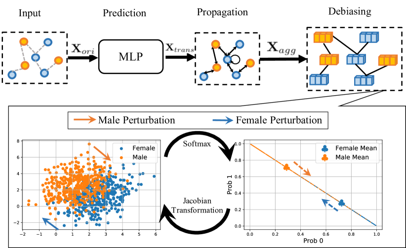
Figure 2: The model pipeline consists of three steps: MLP (feature transformation), propagation with skip connection and debiasing via low-rank perturbation in probability space.

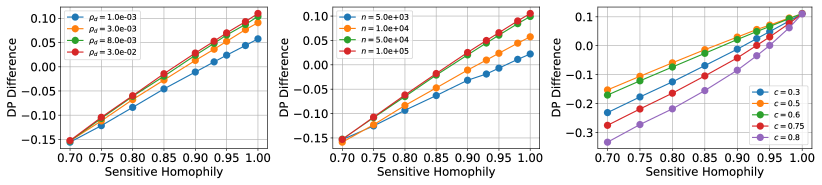
Figure 3: The difference of demographic parity for message passing. Left: DP difference for different graph connection density $\rho_{d}$ with senstive attribute ratio $c=0.5$ and number of nodes $n=10^{4}$; Middle: DP difference for different number of nodes $n$ with senstive attribute ratio $c=0.5$ and graph connection density $\rho_{d}=10^{-3}$; Right: DP difference for different senstive attribute ratio $c$ with graph connection density $\rho_{d}=10^{-3}$ and number of nodes $n=10^{4}$;

Gradient Computation.

The softmax property is also adopted to accelerate the gradient computation. Note that $\mathbf{p}=\mathbf{\Delta}_{s}SF(\mathbf{F})$ and $SF(\cdot)$ represents softmax over column dimension, directly computing the gradient $\frac{\partial\langle\mathbf{p},\mathbf{u}\rangle}{\partial\mathbf{F}}$ based on chain rule involves the three-dimensional tensor $\frac{\partial\mathbf{p}}{\partial\mathbf{F}}$ with gigantic computation complexity. Instead, we simplify the gradient computation based on the property of softmax function in the following theorem.

Theorem 3 (Gradient Computation).

The gradient over primal variable $\frac{\partial\langle\mathbf{p},\mathbf{u}\rangle}{\partial\mathbf{F}}$ satisfies

$$\frac{\partial\langle\mathbf{p},\mathbf{u}\rangle}{\partial\mathbf{F}}=\mathbf{U}_{s}\odot SF(\mathbf{F})-\text{Sum}_{1}(\mathbf{U}_{s}\odot SF(\mathbf{F}))SF(\mathbf{F}).$$ (9)

where $\mathbf{U}_{s}\stackrel{{\scriptstyle\triangle}}{{=}}\Delta_{s}^{\top}\mathbf{u}$, $\odot$ represents element-wise product and $\text{Sum}_{1}(\cdot)$ represents the summation over column dimension with preserved matrix shape.

4.3 FMP Analysis

In this section, we analyze the transparency and efficiency and effectiveness of proposed FMP scheme. Specifically, we intreprete FMP as conventional aggregation plus bias mitigation two phrases, and the computation complexity of FMP is lower than backward gradient calculation.

Transparency

Note that the gradient of fairness objective over node features $\mathbf{F}$ satisfies $\frac{\partial\langle\mathbf{p},\mathbf{u}\rangle}{\partial\mathbf{F}}=\frac{\partial\langle\mathbf{p},\mathbf{u}\rangle}{\partial SF(\mathbf{F})}\frac{\partial SF(\mathbf{F})}{\partial\mathbf{F}}$ and $\frac{\partial\langle\mathbf{p},\mathbf{u}\rangle}{\partial SF(\mathbf{F})}=\Delta_{s}^{\top}\mathbf{u}$, such gradient calculation can be interpreted as three steps: Softmax transformation, pertubation in probability space, and debiasing in representation space. Specifcally, we first map the node representation into probability space via softmax transformation. Subsequently, we calculate the gradient of fairness objective in probability space. It is seen that the pertubation $\Delta_{s}^{\top}\mathbf{u}$ actually poses low-rank debiasing in probability space, where the nodes with different sensitive attribute embrace opposite pertubation. In other words, the dual variable $\mathbf{u}$ represents the pertubation direction in probability space. Finally, the pertubation in probability space will be transformed into representation space via Jacobian transformation $\frac{\partial SF(\mathbf{F})}{\partial\mathbf{F}}$.

Efficiency

FMP is an efficient message passing scheme. The computation complexity for the aggregation (sparse matrix multiplications) is $O(md_{out})$, where $m$ is the number of edges in the graph. For FMP, the extra computation mainly focus on the perturbation calculation, as shown in Theorem 3, with the computation complexity $O(nd_{out})$. The extra computation complexity is negligible in that the number of nodes $n$ is far less than the number of edges $m$ in the real-world graph. Additionally, if directly adopting autograd to calculate the gradient via back propagation, we have to calculate the three-dimensional tensor $\frac{\partial\mathbf{p}}{\partial\mathbf{F}}$ with computation complexity $O(n^{2}d_{out})$. In other words, thanks to the softmax property, we achieve an efficient fair message passing scheme.

Effectiveness

The proposed FMP explicitly achieves graphs smoothness prior and fairness via alternative gradient descent. In other words, the propagation and debiasing forward in a white-box manner and there is not any trainable weight during forwarding phrase. The effectiveness of the proposed FMP is also validated in the experiments on three real-world datasets.

Table 1: Comparative Results with Baselines on Node Classification.

Models	Pokec-z			Pokec-n			NBA
	Acc ($\%$) $\uparrow$	$\Delta_{DP}$ ($\%$) $\downarrow$	$\Delta_{EO}$ ($\%$) $\downarrow$	Acc ($\%$) $\uparrow$	$\Delta_{DP}$ ($\%$) $\downarrow$	$\Delta_{EO}$ ($\%$) $\downarrow$	Acc ($\%$) $\uparrow$	$\Delta_{DP}$ ($\%$) $\downarrow$	$\Delta_{EO}$ ($\%$) $\downarrow$
MLP	70.48 $\pm$ 0.77	1.61 $\pm$ 1.29	2.22 $\pm$ 1.01	72.48 $\pm$ 0.26	1.53 $\pm$ 0.89	3.39 $\pm$ 2.37	65.56 $\pm$ 1.62	22.37 $\pm$ 1.87	18.00 $\pm$ 3.52
GAT	69.76 $\pm$ 1.30	2.39 $\pm$ 0.62	2.91 $\pm$ 0.97	71.00 $\pm$ 0.48	3.71 $\pm$ 2.15	7.50 $\pm$ 2.88	57.78 $\pm$ 10.65	20.12 $\pm$ 16.18	13.00 $\pm$ 13.37
GCN	71.78 $\pm$ 0.37	3.25 $\pm$ 2.35	2.36 $\pm$ 2.09	73.09 $\pm$ 0.28	3.48 $\pm$ 0.47	5.16 $\pm$ 1.38	61.90 $\pm$ 1.00	23.70 $\pm$ 2.74	17.50 $\pm$ 2.63
SGC	71.24 $\pm$ 0.46	4.81 $\pm$ 0.30	4.79 $\pm$ 2.27	71.46 $\pm$ 0.41	2.22 $\pm$ 0.29	3.85 $\pm$ 1.63	63.17 $\pm$ 0.63	22.56 $\pm$ 3.94	14.33$\pm$ 2.16
APPNP	66.91 $\pm$ 1.46	3.90 $\pm$ 0.69	5.71 $\pm$ 1.29	69.80 $\pm$ 0.89	1.98 $\pm$ 1.30	4.01 $\pm$ 2.36	63.80 $\pm$ 1.19	26.51 $\pm$ 3.33	20.00 $\pm$ 4.56
FMP	70.50 $\pm$ 0.50	0.81 $\pm$ 0.40	1.73 $\pm$ 1.03	72.16 $\pm$ 0.33	0.66 $\pm$ 0.40	1.47 $\pm$ 0.87	73.33 $\pm$ 1.85	18.92 $\pm$ 2.28	13.33 $\pm$ 5.89

5 Experiments

In this section, we conduct experiments to validate the effectiveness and efficiency (see Apppendix K for more details.) of proposed FMP. We firstly validate that graph data with large sensitive homophily enhances bias in GNNs via synthetic experiments. Moreover, for experiments on real-world datasets, we introduce the experimental settings and then evaluate our proposed FMP compared with several baselines interms of prediction performance and fairness metrics.

5.1 Synthetic Experiments

We investigate the influence of graph node number $n$, graph connection density $\rho_{d}$, sensitive homophily $\epsilon_{sens}$, and sensitive attribute ration $c$ for bias enhancement of GCN-like message passing. For evaluation metric, we adopt the demographic parity (DP) difference during message passing to measure the bias enhancement. For node attribute generation, we first generate node attribute with Gaussian distribution $\mathcal{N}(\mathbf{\mu}_{1},\mathbf{\Sigma})$ and $\mathcal{N}(\mathbf{\mu}_{2},\mathbf{\Sigma})$ for node with binary sensitive attribute, respectively, where $\mathbf{\mu}_{1}=[0,1]$, $\mathbf{\mu}_{1}=[1,0]$ and $\mathbf{\Sigma}=\left[{\begin{array}[]{cc}1&0\\ 0&1\\ \end{array}}\right]$. For adjacency matrix generation, we randomly generate edges via stochastic block model based on the intra-connection and inter-connection probability.

Figure3 shows the DP difference during message passing with respect to sensitive homophily coefficient. We observe that higher sensitive homophily coefficient generally leads to larger bias enhancement. Additionally, higher graph connection density $\rho_{d}$, larger node number $n$, and balanced sensitive attribute ratio $c$ corresponds higher bias enhancement, which is consistent to our theoretical analysis in Theorem 2.

5.2 Experiments on Real-World Datasets

5.2.1 Experimental Settings

Datasets.

We conduct experiments on real-world datasets Pokec-z, Pokec-n, and NBA (Dai & Wang, 2021). Pokec-z and Pokec-n are sampled, based on province information, from a larger Facebook-like social network Pokec (Takac & Zabovsky, 2012) in Slovakia, where region information is treated as the sensitive attribute and the predicted label is the working field of the users. NBA dataset is extended from a Kaggle dataset consisting of around 400 NBA basketball players. The information of players includes age, nationality, and salary in the 2016-2017 season. The players’ link relationships is from Twitter with the official crawling API. The binary nationality (U.S. and overseas player) is adopted as the sensitive attribute and the prediction label is whether the salary is higher than the median.

Evaluation Metrics.

We adopt accuracy to evaluate the performance of node classification task. As for fairness metric, we adopt two quantitative group fairness metrics to measure the prediction bias. According to works (Louizos et al., 2015; Beutel et al., 2017), we adopt demographic parity $\Delta_{DP}=|\mathbb{P}(\hat{y}=1|s=-1)-\mathbb{P}(\hat{y}=1|s=1)|$ and equal opportunity $\Delta_{DP}=|\mathbb{P}(\hat{y}=1|s=-1,y=1)-\mathbb{P}(\hat{y}=1|s=1,y=1)|$, where $y$ and $\hat{y}$ represent the ground-truth label and predicted label, respectively.

Baselines.

We compare our proposed FMP with representative GNNs, such as GCN (Kipf & Welling, 2017), GAT (Veličković et al., 2018), SGC (Wu et al., 2019), and APPNP (Klicpera et al., 2019), and MLP. For all models, we train 2 layers neural networks with 64 hidden units for $300$ epochs. Additionally, We also compare adversarial debiasing and adding demographic regularization methods to show the effectiveness of the proposed method.

Implementation Details.

We run the experiments $5$ times and report the average performance for each method. We adopt Adam optimizer with $0.001$ learning rate and $1e^{-5}$ weight decay for all models. For adversarial debiasing, we adopt train classifier and adversary with $70$ and $30$ epochs, respectively. The hyperprameter for adversary loss is tuned in $\{0.0,1.0,2.0,5.0,8.0,10.0,20.0,30.0\}$. For adding regularization, we adopt the hyperparameter set $\{0.0,1.0,2.0,5.0,8.0,10.0,20.0,50.0,80.0,100.0\}$.

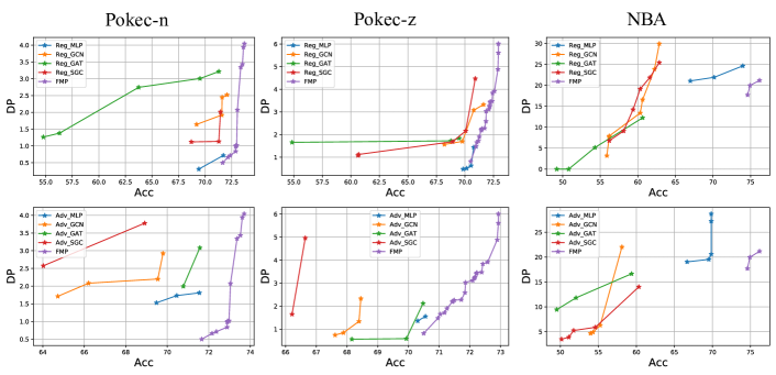
Figure 4: DP and Acc trade-off performance on three real-world datasets compared with adding regularization (Top) and adversarial debiasing (Bottom). The trade-off curve more close to right bottom corner means better trade-off performance.

5.2.2 Experimental Results

Comparison with existng GNNs.

The accuracy, demographic parity and equal opportunity metrics of proposed FMP for Pokec-z, Pokec-n, NBA dataset are shown in Table 1 compared with MLP, GAT, GCN, SGC and APPNP. The detailed statistical information for these three dataset is shown in Table  3. From these results, we can obtain the following observations:

• Many existing GNNs underperorm MLP model on all three datasets in terms of fairness metric. For instance, the demographic parity of MLP is lower than GAT, GCN, SGC and APPNP by $32.64\%$, $50.46\%$, $66.53\%$ and $58.72\%$ on Pokec-z dataset. The higher prediction bias comes from the aggregation within the-same-sensitive-attribute nodes and topology bias in graph data.

• Our proposed FMP consistently achieve lowest prediction bias in terms of demographic parity and equal opportunity on all datasets. Specifically, FMP reduces demographic parity by $49.69\%$, $56.86\%$ and $5.97\%$ compared with the lowest bias among all baselines in Pokec-z, Pokec-n, and NBA dataset. Meanwhile, our proposed FMP achieves the best accuracy in NBA dataset, and comparable accuracy in Pokec-z and Pokec-n datasets. In a nutshell, proposed FMP can effectively mitigate prediction bias while preserving the prediction performance.

Comparison with adversarial debiasing and regularization.

To validate the effectiveness of proposed FMP, we also show the prediction performance and fairness metric trade-off compared with fairness-boosting methods, including adversarial debiasing (Fisher et al., 2020) and adding regularization (Chuang & Mroueh, 2020). Similar to (Louppe et al., 2017), the output of GNNs is the input of adversary and the goal of adversary is to predict the node sensitive attribute. We also adopt several backbones for these two methods, including MLP, GCN, GAT and SGC. We randomly split $50\%/25\%/25\%$ for training, validation and test dataset. Figure 4 shows the pareto optimality curve for all methods, where right-bottom corner point represents the ideal performance (highest accuracy and lowest prediction bias). From the results, we list the following observations as follows:

• Our proposed FMP can achieve better DP-Acc trade-off compared with adversarial debiasing and adding regularization for many GNNs and MLP. Such observation validates the effectiveness of the key idea in FMP: aggregation first and then debiasing. Additionally, FMP can reduce demographic parity with negligible performance cost due to transparent and efficient debiasing.

• Message passing in GNNs does matter. For adding regularization or adversarial debiasing, different GNNs embrace huge distinction, which implies that appropriate message passing manner potentially leads to better trade-off performance. Additionally, many GNNs underperforms MLP in low label homophily coefficient dataset, such as NBA. The rationale is that aggregation may not always bring benefit in terms of accuracy when the neighbors have low probability with the same label.

6 Related Works

Due to the page limit, we briefly review the existing work on graph neural networks and fairness-aware learning on graphs. A more comprehensive discussion can be found in Appendix J. Existing GNNs can be roughly divided into spectral-based and spatial-based GNNs. Spectral-based GNNs provide graph convolution definition based on graph theory (Bruna et al., 2013; Defferrard et al., 2016; Henaff et al., 2015). Spatial-based GNNs variant are popular due to explicit neighbors’ information aggregation, including Graph con-volutional networks (GCN) (Kipf & Welling, 2017), graph attention network (GAT) (Veličković et al., 2018). The unified optimization framework are also provided to unify many existing message passing schemes (Ma et al., 2021c). As for fairness in graph data, many works have been developed to achieve fairness in machine learning community (Chuang & Mroueh, 2020), including fair walk (Rahman et al., 2019), adversarial debiasin (Dai & Wang, 2021), Bayesian approach (Buyl & De Bie, 2020), and contrastive learning (Agarwal et al., 2021). However, aforementioned works ignore the role of message passing in terms of fairness. In this work, we theoretically and experimentally reveal that GNNs aggregation schemes enhance node representation bias under topology bias, and develop a efficient and transparent fair message passing scheme via utilizing useful information of neighbors and debiasing node representation simultaneously.

7 Conclusion

In this work, we theoretically demonstrate that the message passing enhances node representations bias under large sensitive homophily coefficient, and reveal the role of other graph statistical information in terms of bias enhancement. Additionally, integrated in a unified optimization framework, we develop an efficient, effective and transparent FMP to learn fair node representations while preserving prediction performance. Experimental results on real-world datasets demonstrate the effectiveness and efficiency compared with state-of-the-art baseline in node classification tasks.

Appendix A Notations

Table 2: Table of Notations

Notations	Description
$|\mathcal{E}|$	The number of edges
$n,d,d_{out}$	The number of nodes; the number of node feature dimensions; the number of node classes
$\Delta_{\mathbf{s}}\in\mathbb{R}^{1\times n}$	The sensitive attribute incident vector
$\epsilon_{label}$	Label homophily coefficient
$\epsilon_{sens}$	Sensitive homophily coefficient
$\mathbf{X}_{ori}\in\mathbb{R}^{n\times d}$	The input node attributes matrix
$\mathbf{A}\in\mathbb{R}^{n\times n}$	The adjacency matrix
$\hat{\mathbf{A}}\in\mathbb{R}^{n\times n}$	The adjacency matrix with self-loop
$\tilde{\mathbf{A}}\in\mathbb{R}^{n\times n}$	The normalized adjacency matrix with self-loop
$\mathbf{L}\in\mathbb{R}^{n\times n}$	The Laplacian matrix
$\mathbf{X}_{trans}\in\mathbb{R}^{n\times d_{out}}$	The output node features for feature transformation
$\mathbf{F}_{agg}\in\mathbb{R}^{n\times d_{out}}$	The aggregated node features after propagation
$\mathbf{F}\in\mathbb{R}^{n\times d_{out}}$	The learned node features considering graph smoothness and fairness
$\mathbf{u}\in\mathbb{R}^{1\times d_{out}}$	The permutation direction in feature representation space
$h^{*}(\cdot)$	Fenchel conjugate function of $h(\cdot)$
$||\mathbf{X}||_{F}$, $||\mathbf{X}||_{1}$	The Frobenius norm and $l_{1}$ norm of matrix $\mathbf{X}$
$\lambda_{f}$, $\lambda_{s}$	Hyperparameter for fairness and graph smoothness objectives

Appendix B Proof of Theorem 1

We provide a more general proof for categorical sensitive attribute $\mathbf{s}\in\{1,2,\cdots,K\}$ and the prior probability is given by $\mathbb{P}(\mathbf{s}=i)=c_{i}$. Suppose the conditional node attribute $\mathbf{x}$ distribution given node sensitive attribute $\mathbf{s}=i$ satisfies normal distribution $P_{i}(\mathbf{x})\stackrel{{\scriptstyle\triangle}}{{=}}\mathcal{N}(\mathbf{\mu}_{i},\mathbf{\Sigma_{i}})$, the distribution of node sensitive attribute is the mixed Gaussian distribution $f(\mathbf{x})=\sum_{i=1}^{K}c_{i}P_{i}(\mathbf{x})$. Based on the definition of mutual information, we have

$$I(\mathbf{s},\mathbf{x})=H(\mathbf{x})-\sum_{i=1}^{K}c_{i}H(\mathbf{x}|\mathbf{s}=i);$$ (10)

where $H(\cdot)$ represents Shannon entropy for random variable. Subsequently, we focus on the entropy of the mixed Gaussian distribution $H(\mathbf{x})$. We show that such entropy can be upper bounded by the pairwise Kullback-Leibler (KL) divergence as follows:

$$I(\mathbf{s},\mathbf{x}) = -\sum_{i=1}^{K}c_{i}\mathbb{E}_{P_{i}}\big{[}\ln\sum_{j=1}^{K}c_{j}P_{j}(\mathbf{x})\big{]}-\sum_{i=1}^{K}c_{i}H(\mathbf{x}|\mathbf{s}=i)$$

$$\overset{(a)}{\leq} -\sum_{i=1}^{K}c_{i}\big{[}\ln\sum_{j=1}^{K}c_{j}e^{\mathbb{E}_{P_{i}}[\ln P_{j}(\mathbf{x})]}\big{]}-\sum_{i=1}^{K}c_{i}H(\mathbf{x}|\mathbf{s}=i)$$

$$= -\sum_{i=1}^{K}c_{i}\big{[}\ln\sum_{j=1}^{K}c_{j}e^{-H(P_{i}||P_{j})}\big{]}-\sum_{i=1}^{K}c_{i}H(\mathbf{x}|\mathbf{s}=i)$$

$$\overset{(b)}{=} -\sum_{i=1}^{K}c_{i}\big{[}\ln\sum_{j=1}^{K}c_{j}e^{-H(P_{i})-D_{KL}(P_{i}||P_{j})}\big{]}-\sum_{i=1}^{K}c_{i}H(\mathbf{x}|\mathbf{s}=i)$$

$$= -\sum_{i=1}^{K}c_{i}\big{[}\ln\sum_{j=1}^{K}c_{j}e^{-D_{KL}(P_{i}||P_{j})}\big{]},$$

where KL divergence $D_{KL}(P_{i}||P_{j})\stackrel{{\scriptstyle\triangle}}{{=}}\int P_{i}(\mathbf{x})\ln\frac{P_{i}(\mathbf{x})}{P_{j}(\mathbf{x})}\mathrm{d}\mathbf{x}$ and cross entropy $H(P_{i}||P_{j})=-\int P_{i}(\mathbf{x})\ln P_{j}(\mathbf{x})\mathrm{d}\mathbf{x}$. The inequality (a) holds based on the variational lower bound on the expectation of a log-sum inequality $\mathbb{E}\big{[}\ln\sum_{i}Z_{i}\big{]}\geq\ln\big{[}\sum_{i}e^{\mathbb{E}[\ln Z_{i}]}\big{]}$ (Kullback, 1997), and quality $(2)$ holds based on $H(P_{i}||P_{j})=H(P_{i})+D_{KL}(P_{i}||P_{j})$. As a special case for binary sensitive attribute, it is easy to obtain the following results:

$$I(\mathbf{s},\mathbf{X})\leq-(1-c)\ln\Big{[}(1-c)+c\exp\big{(}-D_{KL}(P_{1}||P_{2})\big{)}\Big{]}-c\ln\Big{[}c+(1-c)\exp\big{(}-D_{KL}(P_{2}||P_{1})\big{)}\Big{]}.$$

Appendix C Proof of Theorem 2

Before going deeper for our proof, we first introduce two useful lemmas on KL divergence and statistical information of graph.

Lemma 1.

For two $d$-dimensional Gaussian distributions $P=\mathcal{N}(\mathbf{\mu}_{p},\mathbf{\Sigma}_{p})$ and $Q=\mathcal{N}(\mathbf{\mu}_{q},\mathbf{\Sigma}_{q})$, the KL divergence $D_{KL}(P||Q)$ is given by

$$D_{KL}(P||Q)=\frac{1}{2}\Big{[}\ln\frac{|\mathbf{\Sigma}_{q}|}{|\mathbf{\Sigma}_{p}|}-d+(\mathbf{\mu}_{p}-\mathbf{\mu}_{q})^{\top}\mathbf{\Sigma}_{q}^{-1}(\mathbf{\mu}_{p}-\mathbf{\mu}_{q})+Tr(\mathbf{\Sigma}_{q}^{-1}\mathbf{\Sigma}_{p})\Big{]}$$ (11)

where $\top$ is matrix transpose operation and $Tr(\cdot)$ is trace of a square matrix.

Proof.

Note that the probability density function of multivariate Normal distribution is given by:

$$P(\mathbf{x})=\frac{1}{(2\pi)^{d/2}|\mathbf{\Sigma}_{p}|^{1/2}}\exp\Big{(}-\frac{1}{2}(\mathbf{x}-\mathbf{\mu}_{p})^{\top}\mathbf{\Sigma}_{p}^{-1}(\mathbf{x}-\mathbf{\mu}_{p})\Big{)},$$

the KL divergence between distributions $P$ and $Q$ can be given by

$$D_{KL}(P||Q) = \mathbb{E}_{P}[\ln(P)-\ln(Q)]$$ (12)

$$= \mathbb{E}_{P}\Big{[}\frac{1}{2}\ln\frac{|\mathbf{\Sigma}_{q}|}{|\mathbf{\Sigma}_{p}|}-\frac{1}{2}(\mathbf{x}-\mathbf{\mu}_{p})^{\top}\mathbf{\Sigma}_{p}^{-1}(\mathbf{x}-\mathbf{\mu}_{p})+\frac{1}{2}(\mathbf{x}-\mathbf{\mu}_{q})^{\top}\mathbf{\Sigma}_{q}^{-1}(\mathbf{x}-\mathbf{\mu}_{q})\Big{]}$$

$$= \frac{1}{2}\ln\frac{|\mathbf{\Sigma}_{q}|}{|\mathbf{\Sigma}_{p}|}-\underbrace{\frac{1}{2}\mathbb{E}_{P}\Big{[}(\mathbf{x}-\mathbf{\mu}_{p})^{\top}\mathbf{\Sigma}_{p}^{-1}(\mathbf{x}-\mathbf{\mu}_{p})\Big{]}}_{I_{1}}+\underbrace{\frac{1}{2}\mathbb{E}_{P}\Big{[}(\mathbf{x}-\mathbf{\mu}_{q})^{\top}\mathbf{\Sigma}_{q}^{-1}(\mathbf{x}-\mathbf{\mu}_{q})\Big{]}}_{I_{2}}.$$

Using the commutative property of the trace operation, we have

$$I_{1} = \frac{1}{2}\mathbb{E}_{P}\Big{[}(\mathbf{x}-\mathbf{\mu}_{p})^{\top}\mathbf{\Sigma}_{p}^{-1}(\mathbf{x}-\mathbf{\mu}_{p})\Big{]}=\frac{1}{2}Tr\Big{(}\mathbb{E}_{P}\Big{[}(\mathbf{x}-\mathbf{\mu}_{p})^{\top}(\mathbf{x}-\mathbf{\mu}_{p})\mathbf{\Sigma}_{p}^{-1}\Big{]}\Big{)}$$ (13)

$$= \frac{1}{2}Tr\Big{(}\mathbb{E}_{P}\Big{[}(\mathbf{x}-\mathbf{\mu}_{p})^{\top}(\mathbf{x}-\mathbf{\mu}_{p})\Big{]}\mathbf{\Sigma}_{p}^{-1}\Big{)}=\frac{1}{2}Tr\Big{(}\mathbf{\Sigma}_{p}\mathbf{\Sigma}_{p}^{-1}\Big{)}=\frac{d}{2},$$

As for the term $I_{2}$, note that $\mathbf{x}-\mathbf{\mu}_{q}=(\mathbf{x}-\mathbb{E}_{P}[\mathbf{x}])+(\mathbb{E}_{P}[\mathbf{x}]-\mathbf{\mu}_{q})$, we can obtain the following equation:

$$I_{2} = \frac{1}{2}\mathbb{E}_{P}\Big{[}(\mathbf{x}-\mathbf{\mu}_{q})^{\top}\mathbf{\Sigma}_{q}^{-1}(\mathbf{x}-\mathbf{\mu}_{q})\Big{]}$$ (14)

$$= \frac{1}{2}\Big{[}(\mathbf{\mu}_{p}-\mathbf{\mu}_{q})^{\top}\mathbf{\Sigma}_{q}^{-1}(\mathbf{\mu}_{p}-\mathbf{\mu}_{q})+Tr(\mathbf{\Sigma}_{q}^{-1}\mathbf{\Sigma}_{p})\Big{]},$$

Therefore, the KL divergence $D_{KL}(P||Q)$ is given by

$$D_{KL}(P||Q)=\frac{1}{2}\Big{[}\ln\frac{|\mathbf{\Sigma}_{q}|}{|\mathbf{\Sigma}_{p}|}-d+(\mathbf{\mu}_{p}-\mathbf{\mu}_{q})^{\top}\mathbf{\Sigma}_{q}^{-1}(\mathbf{\mu}_{p}-\mathbf{\mu}_{q})+Tr(\mathbf{\Sigma}_{q}^{-1}\mathbf{\Sigma}_{p})\Big{]}.$$ (15)

∎

Lemma 2.

Suppose the synthetic graph is generated from $(n,\rho_{d},\epsilon_{sens},c)$-graph, then we obtain the intra-connect and inter-connect probability as follows:

$$p_{conn}=\frac{\rho_{d}\epsilon_{sens}}{c^{2}+(1-c)^{2}},\quad q_{conn}=\frac{\rho_{d}(1-\epsilon_{sens})}{2c(1-c)}.$$

Proof.

Based on Bayes’ rule, we have the intra-connect and inter-connect probability as follows

$$p_{conn}=\mathbb{P}(\mathbf{A}_{ij}=1|\mathbf{s}_{i}=\mathbf{s}_{j})=\frac{\mathbb{P}(\mathbf{A}_{ij}=1)\mathbb{P}(\mathbf{s}_{i}=\mathbf{s}_{j}|\mathbf{A}_{ij}=1)}{\mathbb{P}(\mathbf{s}_{i}=\mathbf{s}_{j})}=\frac{\rho_{d}\epsilon_{sens}}{c^{2}+(1-c)^{2}},$$

$$q_{conn}=\mathbb{P}(\mathbf{A}_{ij}=1|\mathbf{s}_{i}\mathbf{s}_{j}=-1)=\frac{\mathbb{P}(\mathbf{A}_{ij}=1)\mathbb{P}(\mathbf{s}_{i}\mathbf{s}_{j}=-1|\mathbf{A}_{ij}=1)}{\mathbb{P}(\mathbf{s}_{i}\mathbf{s}_{j})=-1}=\frac{\rho_{d}(1-\epsilon_{sens})}{2c(1-c)}.$$ (16)

∎

Note that the synthetic graph is generated from $(n,\rho_{d},\epsilon_{sens},c)$-graph. The sensitive attribute $\mathbf{s}$ is generated to with ratio $c$, i.e., the number of node sensitive attribute $\mathbf{s}=-1$ and $\mathbf{s}=1$ are $n_{-1}=n(1-c)$ and $n_{1}=nc$. Based on the determined sensitive attribute $\mathbf{s}$, we randomly generate the edge based on parameters $\rho_{d}$ and $\epsilon_{sens}$ and Lemma 2, i.e., the edges within and cross the same group are randomly generated based on intra-connect probability and inter-connect probability. Therefore, the adjacency matrix $\mathbf{A}_{ij}$ is independent on node attribute $\mathbf{X}_{i}$ and $\mathbf{X}_{j}$ given sensitive attributes $\mathbf{s}_{i}$ and $\mathbf{s}_{j}$, i.e., $\mathbf{A}_{ij}\perp\!\!\!\perp(\mathbf{X}_{i},\mathbf{X}_{j})|(\mathbf{s}_{i},\mathbf{s}_{j})$. Similarly, the different node attributes and edges are also dependent for each other given sensitive attributes, i.e., $\mathbf{A}_{ij}\perp\!\!\!\perp\mathbf{A}_{ij}|(\mathbf{s}_{i},\mathbf{s}_{j},\mathbf{s}_{k})$ and $\mathbf{X}_{i}\perp\!\!\!\perp\mathbf{X}_{j}|(\mathbf{s}_{i},\mathbf{s}_{j})$. Therefore, considering GCN-like message passing $\tilde{\mathbf{X}}_{i}=\sum_{j=1}^{n}\tilde{\mathbf{A}_{ij}}\mathbf{X}_{j}$, we have the aggregated node attributes expectation given sensitive attribute as follows:

$$\tilde{\mathbf{\mu}}_{1} = \mathbb{E}_{\tilde{\mathbf{X}}_{i}}[\tilde{\mathbf{X}}_{i}|\mathbf{s}_{i}=-1]=\sum_{j=1}^{n}\mathbb{E}_{\tilde{\mathbf{A}}_{ij},\mathbf{X}_{j}}[\tilde{\mathbf{A}}_{ij}\mathbf{X}_{j}|\mathbf{s}_{i}=-1]=\sum_{j=1}^{n}\mathbb{E}_{\tilde{\mathbf{A}}_{ij}}[\tilde{\mathbf{A}}_{ij}|\mathbf{s}_{i}=-1]\mathbf{E}_{\mathbf{X}_{j}}[\mathbf{X}_{j}|\mathbf{s}_{i}=-1]$$ (17)

$$= (n_{-1}-1)\mathbb{E}_{\tilde{\mathbf{A}}_{ij}}[\tilde{\mathbf{A}}_{ij}|\mathbf{s}_{i}=-1,\mathbf{s}_{j}=-1]\mathbf{E}_{\mathbf{X}_{j}}[\tilde{\mathbf{X}}_{j}|\mathbf{s}_{i}=-1,\mathbf{s}_{j}=-1]$$

$$+\mathbb{E}_{\tilde{\mathbf{A}}_{ij}}[\tilde{\mathbf{A}}_{ij}|\mathbf{s}_{i}=-1,i=j]\mathbf{E}_{\mathbf{X}_{j}}[\mathbf{X}_{j}|\mathbf{s}_{i}=-1]$$

$$+n_{1}\mathbb{E}_{\tilde{\mathbf{A}}_{ij}}[\tilde{\mathbf{A}}_{ij}|\mathbf{s}_{i}=-1,\mathbf{s}_{j}=1]\mathbf{E}_{\mathbf{X}_{j}}[\mathbf{X}_{j}|\mathbf{s}_{i}=-1,\mathbf{s}_{j}=1]$$

$$= \frac{[(n_{-1}-1)p_{conn}+1]\mathbf{\mu}_{1}+n_{1}q_{conn}\mathbf{\mu}_{2}}{(n_{-1}-1)p_{conn}+1+n_{1}q_{conn}}\stackrel{{\scriptstyle\triangle}}{{=}}\nu_{1}\mathbf{\mu}_{1}+(1-\nu_{1})\mathbf{\mu}_{2}.$$

where $\nu_{1}=\frac{(n_{-1}-1)p_{conn}+1}{(n_{-1}-1)p_{conn}+1+n_{1}q_{conn}}$. Similarly, for the node with sensitive attribute $1$, we have

$$\tilde{\mathbf{\mu}}_{2} = \mathbb{E}_{\tilde{\mathbf{X}}_{i}}[\tilde{\mathbf{X}}_{i}|\mathbf{s}_{i}=1]=\sum_{j=1}^{n}\mathbb{E}_{\tilde{\mathbf{A}}_{ij},\mathbf{X}_{j}}[\tilde{\mathbf{A}}_{ij}\mathbf{X}_{j}|\mathbf{s}_{i}=1]=\sum_{j=1}^{n}\mathbb{E}_{\tilde{\mathbf{A}}_{ij}}[\tilde{\mathbf{A}}_{ij}|\mathbf{s}_{i}=1]\mathbf{E}_{\mathbf{X}_{j}}[\mathbf{X}_{j}|\mathbf{s}_{i}=1]$$ (18)

$$= n_{-1}\mathbb{E}_{\tilde{\mathbf{A}}_{ij}}[\tilde{\mathbf{A}}_{ij}|\mathbf{s}_{i}=1,\mathbf{s}_{j}=-1]\mathbf{E}_{\mathbf{X}_{j}}[\mathbf{X}_{j}|\mathbf{s}_{i}=1,\mathbf{s}_{j}=-1]$$

$$+\mathbb{E}_{\tilde{\mathbf{A}}_{ij}}[\tilde{\mathbf{A}}_{ij}|\mathbf{s}_{i}=1,i=j]\mathbf{E}_{\mathbf{X}_{j}}[\mathbf{X}_{j}|\mathbf{s}_{i}=1]$$

$$+(n_{1}-1)\mathbb{E}_{\tilde{\mathbf{A}}_{ij}}[\tilde{\mathbf{A}}_{ij}|\mathbf{s}_{i}=1,\mathbf{s}_{j}=1]\mathbf{E}_{\mathbf{X}_{j}}[\mathbf{X}_{j}|\mathbf{s}_{i}=1,\mathbf{s}_{j}=1]$$

$$= \frac{n_{-1}q_{conn}\mathbf{\mu}_{1}+[(n_{1}-1)p_{conn}+1]\mathbf{\mu}_{2}}{n_{-1}q_{conn}+(n_{1}-1)p_{conn}+1}\stackrel{{\scriptstyle\triangle}}{{=}}\nu_{2}\mathbf{\mu}_{1}+(1-\nu_{2})\mathbf{\mu}_{2}.$$

where $\nu_{2}=\frac{(n_{-1}-1)q_{conn}}{n_{-1}q_{conn}+1+(n_{1}-1)p_{conn}}$. As for the covariance matrix of aggregated node attributes $\tilde{\mathbf{X}}$ given node sensitive attribute $\mathbf{s}=-1$ and original sensitive attribute, note that we can obtain

$$\tilde{\mathbf{\Sigma}}_{1} = \mathbb{D}_{\tilde{\mathbf{X}}_{i}}[\tilde{\mathbf{X}}_{i}|\mathbf{s}_{i}=-1]=\sum_{j=1}^{n}\mathbb{D}_{\tilde{\mathbf{A}}_{ij},\mathbf{X}_{j}}[\tilde{\mathbf{A}}_{ij}\mathbf{X}_{j}|\mathbf{s}_{i}=-1]=\sum_{j=1}^{n}\mathbb{E}_{\tilde{\mathbf{A}}_{ij}}[\tilde{\mathbf{A}}_{ij}^{2}|\mathbf{s}_{i}=-1]\mathbf{D}_{\tilde{\mathbf{X}}_{j}}[\tilde{\mathbf{X}}_{j}|\mathbf{s}_{i}=-1]$$ (19)

$$= \frac{(n_{-1}-1)p_{conn}\mathbf{\Sigma}+\mathbf{\Sigma}+n_{1}q_{conn}\mathbf{\Sigma}}{[(n_{-1}-1)p_{conn}+1+n_{1}q_{conn}]^{2}}=\frac{\mathbf{\Sigma}}{(n_{-1}-1)p_{conn}+1+n_{1}q_{conn}}\stackrel{{\scriptstyle\triangle}}{{=}}\zeta_{1}^{-1}\mathbf{\Sigma},$$

where $\zeta_{1}=(n_{-1}-1)p_{conn}+1+n_{1}q_{conn}$. Similarly, given node sensitive attribute $\mathbf{s}=1$, we have $\tilde{\mathbf{\Sigma}}_{2}=\mathbb{D}_{\tilde{\mathbf{X}}_{i}}[\tilde{\mathbf{X}}_{i}|\mathbf{s}_{i}=1]=\frac{\mathbf{\Sigma}}{n_{-1}q_{conn}+1+(n_{1}-1)p_{conn}}\stackrel{{\scriptstyle\triangle}}{{=}}\zeta_{2}^{-1}\mathbf{\Sigma}$, where $\zeta_{2}=n_{-1}q_{conn}+1+(n_{1}-1)p_{conn}$. In other words, the covariance matrix of the aggregated node attributes is lower than original one since “average” operation will make node representation more concentrated. Note that the summation over several Gaussian random variables is still Gaussian, we define the node attributes distribution for sensitive attribute $\mathbf{s}=-1$ and $\mathbf{s}=1$ as $P_{1}=\mathcal{N}(\mathbf{\mu}_{1},\mathbf{\Sigma})$, $P_{2}=\mathcal{N}(\mathbf{\mu}_{2},\mathbf{\Sigma})$, respectively. Similarly, the aggregated node representation distribution follows for sensitive attribute $\mathbf{s}=-1$ and $\mathbf{s}=1$ as $\tilde{P}_{1}=\mathcal{N}(\tilde{\mathbf{\mu}}_{1},\tilde{\mathbf{\Sigma}}_{1})$, $\tilde{P}_{2}=\mathcal{N}(\tilde{\mathbf{\mu}}_{2},\tilde{\mathbf{\Sigma}}_{2})$. Note that the sensitive attribute ratio keeps the same after the aggregation and lager KL divergence for these two sensitive attributes group distribution, the bias enhances $\Delta Bias>0$ if $D_{KL}(\tilde{P}_{1}||\tilde{P}_{2})>D_{KL}(P_{1}||P_{2})$ and $D_{KL}(\tilde{P}_{2}||\tilde{P}_{1})>D_{KL}(P_{2}||P_{1})$. There fore, we only focus on the KL divergence. According to Lemma 1, it is easy to obtain KL divergence for original distribution as follows:

$$D_{KL}(P_{1}||P_{2})=\frac{1}{2}\Big{[}\ln\frac{|\mathbf{\Sigma}|}{|\mathbf{\Sigma}|}-d+(\mathbf{\mu}_{1}-\mathbf{\mu}_{2})^{\top}\mathbf{\Sigma}^{-1}(\mathbf{\mu}_{1}-\mathbf{\mu}_{2})+Tr(\mathbf{\Sigma}^{-1}\mathbf{\Sigma})\Big{]}=\frac{1}{2}(\mathbf{\mu}_{1}-\mathbf{\mu}_{2})^{\top}\mathbf{\Sigma}^{-1}(\mathbf{\mu}_{1}-\mathbf{\mu}_{2}),$$ (20)

As for KL divergence for aggregated distribution, similarly, we have

$$D_{KL}(\tilde{P}_{1}||\tilde{P}_{2}) = \frac{1}{2}\Big{[}\ln\frac{|\tilde{\mathbf{\Sigma}}_{2}|}{|\tilde{\mathbf{\Sigma}}_{1}|}-d+(\tilde{\mathbf{\mu}}_{1}-\tilde{\mathbf{\mu}}_{2})^{\top}\tilde{\mathbf{\Sigma}}_{2}^{-1}(\tilde{\mathbf{\mu}}_{1}-\tilde{\mathbf{\mu}}_{2})+Tr(\tilde{\mathbf{\Sigma}}_{2}^{-1}\tilde{\mathbf{\Sigma}}_{1})\Big{]}$$ (21)

$$= \frac{1}{2}\Big{[}d\ln\frac{\zeta_{1}}{\zeta_{2}}-d+(\nu_{1}-\nu_{2})^{2}\zeta_{2}(\mathbf{\mu}_{1}-\mathbf{\mu}_{2})^{\top}\mathbf{\Sigma}^{-1}(\mathbf{\mu}_{1}-\mathbf{\mu}_{2})+\frac{\zeta_{2}}{\zeta_{1}}Tr(\mathbf{I}_{d})\Big{]}$$

$$\overset{(c)}{\geq} \frac{1}{2}(\nu_{1}-\nu_{2})^{2}\zeta_{2}(\mathbf{\mu}_{1}-\mathbf{\mu}_{2})^{\top}\mathbf{\Sigma}^{-1}(\mathbf{\mu}_{1}-\mathbf{\mu}_{2}),$$

where inequality $(c)$ holds since $\ln x\leq x-1$ for any $x>0$. Compared with equations (20) and (21), it is seen that $D_{KL}(\tilde{P}_{1}||\tilde{P}_{2})>D_{KL}(P_{1}||P_{2})$ if $(\nu_{1}-\nu_{2})^{2}\zeta_{2}>1$. Similarly, we can have $D_{KL}(\tilde{P}_{2}||\tilde{P}_{1})>D_{KL}(P_{2}||P_{1})$ if $(\nu_{1}-\nu_{2})^{2}\zeta_{1}>1$. In a nutshell, the bias enhances $\Delta Bias>0$ after message passing if $(\nu_{1}-\nu_{2})^{2}\min\{\zeta_{1},\zeta_{2}\}>1$.

Appendix D More Details on FMP Derivation

D.1 Proof on Fairness Objective

The fairness objective can be shown as the average prediction probability difference as follows:

$$\Big{(}\Delta_{s}SF(\mathbf{F})\big{)}\Big{)}_{j} = \Big{[}\frac{\mathbbm{1}_{>0}(\mathbf{s})}{||\mathbbm{1}_{>0}(\mathbf{s})||_{1}}-\frac{\mathbbm{1}_{>0}(-\mathbf{s})}{||\mathbbm{1}_{>0}(-\mathbf{s})||_{1}}\Big{]}\big{(}SF(\mathbf{F})\big{)}_{:,j}$$

$$= \frac{\sum_{\mathbf{s}_{i}=1}\hat{P}(y_{i}=j|\mathbf{X})}{||\mathbbm{1}_{>0}(\mathbf{s})||_{1}}-\frac{\sum_{\mathbf{s}_{i}=-1}\hat{P}(y_{i}=j|\mathbf{X})}{||\mathbbm{1}_{>0}(\mathbf{-s})||_{1}}$$

$$= \hat{P}(y_{i}=j|\mathbf{s}_{i}=1,\mathbf{X})-\hat{P}(y_{i}=j|\mathbf{s}_{i}=-1,\mathbf{X}).$$

D.2 Fenchel Conjugate

Fenchel conjugate (Rockafellar, 2015) (a.k.a. convex conjugate) is the key tool to transform the original problem into bi-level optimization problem. For the general convex function $h(\cdot)$, its conjugate function is defined as

$$h^{*}(\mathbf{U})\stackrel{{\scriptstyle\triangle}}{{=}}\sup\limits_{\mathbf{X}}\langle\mathbf{U},\mathbf{X}\rangle-h(\mathbf{X}).$$

Based on Fenchel conjugate, the fairness objective can be transformed as variational representation $h_{f}(\mathbf{p})=\sup\limits_{\mathbf{u}}\langle\mathbf{p},\mathbf{u}\rangle-h_{f}^{*}(\mathbf{u})$, where $\mathbf{p}=\mathbf{\Delta}_{s}SF(\mathbf{F})\in\mathbb{R}^{1\times d_{out}}$ is a predicted probability vector for classification. Furthermore, the original optimization problem is equivalent to $\min\limits_{\mathbf{F}}\max\limits_{\mathbf{u}}h_{s}(\mathbf{F})+\langle\mathbf{p},\mathbf{u}\rangle-h_{f}^{*}(\mathbf{u})$, where $\mathbf{u}\in\mathbb{R}^{1\times d_{out}}$ and $h_{f}^{*}(\cdot)$ is the conjugate function of fairness objective $h_{f}(\cdot)$.

D.3 Fair Message Passing Scheme.

Motivated by Proximal Alternating Predictor-Corrector (PAPC) (Loris & Verhoeven, 2011; Chen et al., 2013), the min-max optimization problem (2) can be solved by the following fixed-point equations

$$\left\{\begin{array}[]{l}\mathbf{F}=\mathbf{F}-\nabla h_{s}(\mathbf{F})-\frac{\partial\langle\mathbf{p},\mathbf{u}\rangle}{\partial\mathbf{F}},\\ \mathbf{u}=\text{prox}_{h^{*}_{f}}\big{(}\mathbf{u}+\mathbf{\Delta_{s}}SF(\mathbf{F})\big{)}.\end{array}\right.$$ (24)

where $\text{prox}_{h^{*}_{f}}(\mathbf{u})=\arg\min\limits_{\mathbf{y}}||\mathbf{y}-\mathbf{u}||_{F}^{2}+h^{*}_{f}(\mathbf{u})$. Similar to “predictor-corrector” algorithm (Loris & Verhoeven, 2011), we adopt iterative algorithm to find saddle point for min-max optimization problem. Specifically, starting from $(\mathbf{F}^{k},\mathbf{u}^{k})$, we adopt a gradient descent step on primal variable $\mathbf{F}$ to arrive $(\bar{\mathbf{F}}^{k+1},\mathbf{u}^{k})$ and then followed by a proximal ascent step in the dual variable $\mathbf{u}$. Finally, a gradient descent step on primal variable in point $(\bar{\mathbf{F}}^{k+1},\mathbf{u}^{k})$ to arrive at $(\mathbf{F}^{k+1},\mathbf{u}^{k})$. In short, the iteration can be summarized as

$$\left\{\begin{array}[]{l}\bar{\mathbf{F}}^{k+1}=\mathbf{F}^{k}-\gamma\nabla h_{s}(\mathbf{F}^{k})-\gamma\frac{\partial\langle\mathbf{p},\mathbf{u}^{k}\rangle}{\partial\mathbf{F}}\Big{|}_{\mathbf{F}^{k}},\\ \mathbf{u}^{k+1}=\text{prox}_{\beta h^{*}_{f}}\big{(}\mathbf{u}^{k}+\beta\mathbf{\Delta_{s}}SF(\bar{\mathbf{F}}^{k+1})\big{)},\\ \bar{\mathbf{F}}^{k+1}=\mathbf{F}^{k}-\gamma\nabla h_{s}(\mathbf{F}^{k})-\gamma\frac{\partial\langle\mathbf{p},\mathbf{u}^{k+1}\rangle}{\partial\mathbf{F}}\Big{|}_{\mathbf{F}^{k}}.\\ \end{array}\right.$$ (28)

where $\gamma$ and $\beta$ are the step size for primal and dual variables. Note that the close-form for $\frac{\partial\langle\mathbf{p},\mathbf{u}\rangle}{\partial\mathbf{F}}\in\mathbb{R}^{n\times d_{out}}$ and $\text{prox}_{\beta h^{*}_{f}}(\cdot)$ are still not clear, we will provide the solution on by one.

Proximal Operator.

As for the proximal operators, we provide the close-form in the following proposition:

Proposition 1 (Proximal Operators).

The proximal operators $\text{prox}_{\beta h^{*}_{f}}(\mathbf{u})$ satisfies

$$\text{prox}_{\beta h^{*}_{f}}(\mathbf{u})_{j}=sign(\mathbf{u})_{j}\min\big{(}|\mathbf{u}_{j}|,\lambda_{f}\big{)},$$ (29)

where $sign(\cdot)$ and $\lambda_{f}$ are element-wise sign function and hyperparameter for fairness objective. In other words, such proximal operator is element-wise projection onto $l_{\infty}$ ball with radius $\lambda_{f}$.

FMP Scheme.

Similar to works (Ma et al., 2021c; Liu et al., 2021), choosing $\gamma=\frac{1}{1+\lambda_{f}}$ and $\beta=\frac{1}{2\gamma}$, we have

$$\mathbf{F}^{k}-\gamma\nabla h_{s}(\mathbf{F}^{k}) = \Big{(}(1-\gamma)\mathbf{I}-\gamma\lambda_{f}\tilde{\mathbf{L}}\Big{)}\mathbf{F}^{k}+\gamma\mathbf{X}_{trans},$$ (30)

$$= \gamma\mathbf{X}_{trans}+(1-\gamma)\tilde{\mathbf{A}}\mathbf{F}^{k},$$

Therefore, we can summarize the proposed FMP as two phases, including propagation with skip connection (Step ❶) and bias mitigation (Steps ❷-❺). For bias mitigation, Step ❷ updates the aggregated node features for fairness objective; Steps ❸ and ❹ aim to learn and “reshape” perturbation vector in probability space, respectively. Step ❺ explicitly mitigate the bias of node features based on gradient descent on primal variable. The mathematical formulation is given as follows:

$$\left\{\begin{array}[]{ll}\mathbf{X}_{agg}^{k+1}=\gamma\mathbf{X}_{trans}+(1-\gamma)\tilde{\mathbf{A}}\mathbf{X}^{k},&\text{Step {\char 182}}\\ \bar{\mathbf{F}}^{k+1}=\mathbf{X}_{agg}^{k+1}-\gamma\frac{\partial\langle\mathbf{p},\mathbf{u}^{k}\rangle}{\partial\mathbf{F}}\Big{|}_{\mathbf{F}^{k}},&\text{Step {\char 183}}\\ \bar{\mathbf{u}}^{k+1}=\mathbf{u}^{k}+\beta\mathbf{\Delta_{s}}SF(\bar{\mathbf{F}}^{k+1}),&\text{Step {\char 184}}\\ \mathbf{u}^{k+1}=\min\Big{(}|\bar{\mathbf{u}}^{k+1}|,\lambda_{f}\Big{)}\cdot sign(\bar{\mathbf{u}}^{k+1}),&\text{Step {\char 185}}\\ \mathbf{F}^{k+1}=\mathbf{X}_{agg}^{k+1}-\gamma\frac{\partial\langle\mathbf{p},\mathbf{u}^{k+1}\rangle}{\partial\mathbf{F}}\Big{|}_{\mathbf{F}^{k}}.&\text{Step {\char 186}}\end{array}\right.$$ (36)

where $\mathbf{X}_{agg}^{k+1}$ represents the node features with normal aggregation and skip connection with the transformed input $\mathbf{X}_{trans}$.

Appendix E More Discussions on Message Passing

In this section, we provide more discussion on the influence of $4$ graph data in-formation of graph:the number of nodes $n$, the edge density $\rho_{d}$, sensitive homophily coefficient $\epsilon_{sens}$, and sensitive group ratio $c$ for bias enhancement.

On the sensitive homophily coefficient $\epsilon_{sens}$.

According to Lemma 2, for large sensitive homophily coefficient $\epsilon_{sens}\rightarrow 1$, the inter-connect probability $q_{conn}\rightarrow 0$ and intra-connect probability $p_{conn}$ keeps the maximal value. In this case, based on Theorem 2, it is easy to obtain that $\nu_{1}=1$, $\nu_{2}=0$ and the distance for the mean aggregated node representation will keep the same, i.e., $\tilde{\mathbf{\mu}}_{1}-\tilde{\mathbf{\mu}}_{2}=(\nu_{1}-\nu_{2})(\mathbf{\mu}_{1}-\mathbf{\mu}_{2})=\mathbf{\mu}_{1}-\mathbf{\mu}_{2}$. Additionally, the covariance will be diminished after aggregation since $\zeta_{1}$ and $\zeta_{2}$ are strictly larger than $1$. Therefore, for sufficient large sensitive homophily coefficient $\epsilon_{sens}$, the bias-enhance condition $(\nu_{1}-\nu_{2})^{2}\min\{\zeta_{1},\zeta_{2}\}>1$ holds.

On the graph node number $n$.

For large node number $n$, the mean distance almostly keeps constant since $\nu_{1}\approx\frac{cp_{conn}}{(1-c)q_{conn}+cp_{conn}}$, $\nu_{2}\approx\frac{cq_{conn}}{(1-c)p_{conn}+cq_{conn}}$, and $\zeta_{1},\zeta_{2}$ are almost proportional to node number $n$. Therefore, the bias-enhancement condition can be more easily satisfied and $\Delta Bias$ would be higher for large graph data. The intuition is that, given graph density ratio, large graph data represents higher average degree node. Hence, each aggregated node representation adopt more neighbor’s information with the same sensitive attribute, and thus leads to lower covariance matrix value and higher representation bias.

On the graph connection density $\rho_{d}$.

Based on Lemma 2, inter-connection probability and inter-connection probability are both proportional to graph connection density $\rho_{d}$. Therefore, $\nu_{1}$ and $\nu_{2}$ almost keep constant and the distance of mean node representation is constant as well. As for covariance matrix, message passing leads to more concentrated node representation since $\zeta_{1}$ and $\zeta_{2}$ are larger for higher graph connection density $\rho_{d}$. The rationale is similar with the graph node number: given node number, higher graph connection density $\rho_{d}$ means higher average node degree and each aggregated node representation adopt more neighbor’s information with the same sensitive attribute.

On the sensitive attribute ration $c$.

Based on Lemma 2, it is easy to obtain that, given graph connection density $\rho_{d}$ and graph node number $n$, the intra-connection probability $p_{conn}$ would be high, while low for inter-connection probability $q_{conn}$, if the balanced sensitive attribute. In other words, intra-connection probability $p_{conn}$ (inter-connection probability $q_{conn}$) monotonically decreases (increases) with respect to $|c-\frac{1}{2}|$.

Appendix F Proof of Theorem 3

Before providing in-depth analysis on the gradient computation, we first introduce the softmax function derivative property in the following lemma:

Lemma 3.

For the softmax function with $N$-dimensional vector input $\mathbf{y}=SF(\mathbf{x}):\mathbb{R}^{1\times N}\longrightarrow\mathbb{R}^{1\times N}$, where $y_{j}=\frac{e^{\mathbf{x}_{j}}}{\sum_{k=1}^{N}e^{\mathbf{x}_{k}}}$ for $\forall j\in\{1,2,\cdots,N\}$, the derivative $N\times N$ Jocobian matrix is defined by $[\frac{\partial\mathbf{y}}{\partial\mathbf{x}}]_{ij}=\frac{\partial\mathbf{y}_{i}}{\partial\mathbf{x}_{j}}$. Additionally, Jocobian matrix satisfies $\frac{\partial\mathbf{y}}{\partial\mathbf{x}}=\mathbf{y}\mathbf{I}_{N}-\mathbf{y}^{\top}\mathbf{y}$, where $\mathbf{I}_{N}$ represents $N\times N$ identity matrix and $\top$ denotes the transpose operation for vector or matrix.

Proof.

Considering the gradient for arbitrary $i=j$, according to quotient and chain rule of derivatives, we have

$$\frac{\partial\mathbf{y}_{i}}{\partial\mathbf{x}_{j}}=\frac{e^{\mathbf{x}_{i}}\sum_{k=1}^{N}e^{\mathbf{x}_{k}}-e^{\mathbf{x}_{i}+\mathbf{x}_{j}}}{\big{(}\sum_{k=1}^{N}e^{\mathbf{x}_{k}}\big{)}^{2}}=\frac{e^{\mathbf{x}_{i}}}{\sum_{k=1}^{N}e^{\mathbf{x}_{k}}}\cdot\frac{\sum_{k=1}^{N}e^{\mathbf{x}_{k}}-e^{\mathbf{x}_{i}}}{\sum_{k=1}^{N}e^{\mathbf{x}_{k}}}=\mathbf{y}_{i}(1-\mathbf{y}_{j}),$$ (37)

Similarly, for arbitrary $i\neq j$, the gradient is given by

$$\frac{\partial\mathbf{y}_{i}}{\partial\mathbf{x}_{j}}=\frac{e^{\mathbf{x}_{i}}}{\sum_{k=1}^{N}e^{\mathbf{x}_{k}}}\cdot\frac{-e^{\mathbf{x}_{i}}}{\sum_{k=1}^{N}e^{\mathbf{x}_{k}}}=-\mathbf{y}_{i}\mathbf{y}_{j}.$$ (38)

Combining these two cases, it is easy to verify the Jocobian matrix satisfies $\frac{\partial\mathbf{y}}{\partial\mathbf{x}}=\mathbf{y}\mathbf{I}_{N}-\mathbf{y}^{\top}\mathbf{y}$. ∎

Arming with the derivative property of softmax function, we further investigate the gradient $\frac{\partial\langle\mathbf{p},\mathbf{u}\rangle}{\partial\mathbf{F}}$, where $\mathbf{p}=\mathbf{\Delta}_{s}SF(\mathbf{F})\in\mathbb{R}^{1\times d_{out}}$ and $SF(\cdot)$ and $\mathbf{u}\in\mathbb{R}^{1\times d_{out}}$ is independent with $\mathbf{F}\in\mathbb{R}^{n\times d_{out}}$.

Considering softmax function $SF(\mathbf{x})\in\mathbb{R}^{n\times d}$ is row-wise adopted in node representation matrix, the gradient satisfies $\frac{\partial SF(\mathbf{F})_{i}}{\partial\mathbf{F}_{j}}=\mathbf{0}_{d_{out}\times d_{out}}$ for $i\neq j$. Note that the inner product $\langle\mathbf{p},\mathbf{u}\rangle=\sum_{k=1}^{d_{out}}\mathbf{p}_{k}\mathbf{u}_{k}$, it is easy the obtain the gradient $[\frac{\partial\langle\mathbf{p},\mathbf{u}\rangle}{\partial\mathbf{F}}]_{ij}=\sum_{k=1}^{d_{out}}\frac{\partial\mathbf{p}_{k}}{\partial\mathbf{F}_{ij}}\mathbf{u}_{k}$.

To simply the current notation, we denote $\mathbf{\tilde{F}}\stackrel{{\scriptstyle\triangle}}{{=}}SF(\mathbf{F})$. According to chain rule of derivative, we have

$$\frac{\partial\mathbf{p}_{k}}{\partial\mathbf{F}_{ij}}=\sum_{t=1}^{d_{out}}\frac{\partial\mathbf{p}_{k}}{\partial\tilde{\mathbf{F}}_{tk}}\frac{\partial\tilde{\mathbf{F}}_{tk}}{\partial\mathbf{F}_{ij}}=\sum_{t=1}^{d_{out}}\Delta_{\mathbf{s},t}\frac{\partial\tilde{\mathbf{F}}_{tk}}{\partial\mathbf{F}_{ij}}\overset{(a)}{=}\Delta_{\mathbf{s},i}\frac{\partial\tilde{\mathbf{F}}_{ik}}{\partial\mathbf{F}_{ij}}\overset{(b)}{=}\Delta_{\mathbf{s},i}\tilde{\mathbf{F}}_{ik}[\delta_{kj}-\tilde{\mathbf{F}}_{ij}],$$ (39)

where $\delta_{kj}$ is Dirac function (equals $1$ only if $k=j$, otherwise $0$;), equality (a) holds since softmax function is row-wise operation, and equality (b) is based on Lemma 3. Furthermore, we can obtain the gradient of fairness objective w.r.t. node presentation as follows:

$$[\frac{\partial\langle\mathbf{p},\mathbf{u}\rangle}{\partial\mathbf{F}}]_{ij}=\sum_{k=1}^{d_{out}}\frac{\partial\mathbf{p}_{k}}{\partial\mathbf{F}_{ij}}\mathbf{u}_{k}=\sum_{k=1}^{d_{out}}\Delta_{\mathbf{s},i}\tilde{\mathbf{F}}_{ik}[\delta_{kj}-\tilde{\mathbf{F}}_{ij}]\mathbf{u}_{k}=\Delta_{\mathbf{s},i}\tilde{\mathbf{F}}_{ij}\mathbf{u}_{j}-\Delta_{\mathbf{s},i}\tilde{\mathbf{F}}_{ij}\sum_{k=1}^{d_{out}}\tilde{\mathbf{F}}_{ik}\mathbf{u}_{k}.$$ (40)

Therefore, the matrix formulation is given by

$$\frac{\partial\langle\mathbf{p},\mathbf{u}\rangle}{\partial\mathbf{F}}=\mathbf{U}_{s}\odot SF(\mathbf{F})-\text{Sum}_{1}(\mathbf{U}_{s}\odot SF(\mathbf{F}))SF(\mathbf{F}).$$ (41)

where $\mathbf{U}_{s}\stackrel{{\scriptstyle\triangle}}{{=}}\Delta_{s}^{\top}\mathbf{u}\in\mathbb{R}^{n\times d_{out}}$ and $\text{Sum}_{1}(\cdot)$ represents the summation over column dimension with preserved matrix shape. Therefore, the computation complexity for gradient $\frac{\partial\langle\mathbf{p},\mathbf{u}\rangle}{\partial\mathbf{F}}$ is $O(nd_{out})$.

Appendix G Proof of Proposition 1

We firstly show the conjugate function for general norm function $f(\mathbf{x})=\lambda||\mathbf{x}||$, where $\mathbf{x}\in\mathbf{R}^{1\times d_{out}}$. The conjugate function of $f(\mathbf{x})$ satisfies

$$f^{*}(\mathbf{y})=\left\{\begin{array}[]{lr}0,&||\mathbf{x}||_{*}\leq\lambda,\\ +\infty,&||\mathbf{x}||_{*}>\lambda.\end{array}\right.$$ (44)

where $||\mathbf{x}||_{*}$ is dual norm of the original norm $||\mathbf{x}||$, defined as $||\mathbf{y}||_{*}=\max\limits_{||\mathbf{x}||\leq 1}\mathbf{y}^{\top}\mathbf{x}$. Considering the conjugate function definition $f^{*}(\mathbf{y})=\max\limits_{\mathbf{x}}\mathbf{y}^{\top}\mathbf{x}-\lambda||\mathbf{x}||$ the analysis can be divided as the following two cases:

❶ If $||\mathbf{y}||_{*}\leq\lambda$, according to the definition of dual norm, we have $\mathbf{y}^{\top}\mathbf{x}\leq||\mathbf{x}||||\mathbf{y}||_{*}\leq\lambda||\mathbf{x}||$ for $\forall||\mathbf{x}||$, where the equality holds if and only if $||\mathbf{x}||=0$. Hence, it is easy to obtain $f^{*}(\mathbf{y})=\max\limits_{\mathbf{x}}\mathbf{y}^{\top}\mathbf{x}-\lambda||\mathbf{x}||=0$.

❷ If $||\mathbf{y}||_{*}>\lambda$, note that the dual norm $||\mathbf{y}||_{*}=\max\limits_{||\mathbf{x}||\leq 1}\mathbf{y}^{\top}\mathbf{x}>\lambda$, there exists variables $\hat{\mathbf{x}}$ so that $||\hat{\mathbf{x}}||\leq 1$ and $\hat{\mathbf{x}}^{\top}\mathbf{y}<\lambda$. Therefore, for any constant $t$, we have $f^{*}(\mathbf{y})\geq\mathbf{y}^{\top}(t\mathbf{x})-\lambda||t\mathbf{x}||=t(\mathbf{y}^{\top}\mathbf{x}-\lambda||\mathbf{x}||)\overset{t\rightarrow\infty}{\longrightarrow}\infty$.

Based on aforementioned two cases, it is easy to get the conjugate function for $l_{1}$ norm (the dual norm is $l_{\infty}$), i.e., the conjugate function for $h_{f}(\mathbf{x})=\lambda||\mathbf{x}||_{1}$ is given by

$$h_{f}^{*}(\mathbf{y})=\left\{\begin{array}[]{lr}0,&||\mathbf{x}||_{\infty}\leq\lambda,\\ +\infty,&||\mathbf{x}||_{\infty}>\lambda.\end{array}\right.$$ (47)

Given the conjugate function $h_{f}^{*}(\cdot)$, we further investigate the proximal operators $\text{prox}_{h^{*}_{f}}$. Note that $\text{prox}_{h^{*}_{f}}(\mathbf{u})=\arg\min\limits_{\mathbf{y}}||\mathbf{y}-\mathbf{u}||_{F}^{2}+h^{*}_{f}(\mathbf{u})=\arg\min\limits_{||\mathbf{y}||_{\infty}\leq\lambda_{f}}||\mathbf{y}-\mathbf{u}||_{F}^{2}=\arg\min\limits_{\begin{subarray}{c}\mathbf{y}_{j}\leq\lambda_{f}\\ \forall j\in[d_{out}]\end{subarray}}\sum_{j=1}^{d_{out}}|\mathbf{y}_{j}-\mathbf{u}_{j}|^{2}$, the proximal operator problem can be decomposed as element-wise sub-problem, i.e.,

$$\text{prox}_{h^{*}_{f}}(\mathbf{u})_{j}=\arg\min\limits_{\mathbf{y}_{j}\leq\lambda_{f}}|\mathbf{y}_{j}-\mathbf{u}_{j}|^{2}=sign(\mathbf{u}_{j})\min(|\mathbf{u}_{j}|,\lambda_{f})$$

which completes the proof.

Appendix H Dataset Statistics

For fair comparison with previous work, we perform the node classification task on three real-world dataset, including Pokec-n, Pokec-z, and NBA. The data statistical information on three real-world dataset is provided in Table 3. It is seen that the sensitive homophily are even higher than label homophily coefficient among three real-world dataset, which validates that the real-world dataset are usually with large topology bias.

Table 3: Statistical Information on Datasets

Dataset	$\#$ Nodes	$\#$ Node Features	$\#$ Edges	$\#$ Training Labels	$\#$ Training Sens	Label Homop	Sens Homop
Pokec-n	66569	265	1034094	4398	500	73.23$\%$	95.30$\%$
Pokec-z	67796	276	1235916	5131	500	71.16$\%$	95.06$\%$
NBA	403	95	21242	156	246	39.22$\%$	72.37$\%$

Appendix I More Discussion on GNNs as Graph Signal Denoising

In this section, we provide more examples to show many existing GNNs can be interpreted as graph signal denoising problem, including GAT and APPNP.

GAT.

Feature aggregation in GAT applies the normalized attention coefficient to compute a linear combination of neighbor’s features as $\mathbf{X}_{agg,i}=\sum_{j\in\mathcal{N}(i)}\alpha_{ij}\mathbf{X}_{trans,j}$, where $\alpha_{ij}=softmax_{j}(e_{ij})$, $e_{ij}=\text{LeakyReLU}(\mathbf{X}_{trans,i}^{\top}\mathbf{w}_{i}+\mathbf{X}_{trans,j}^{\top}\mathbf{w}_{j})$, and $\mathbf{w}_{i}$ and $\mathbf{w}_{j}$ are learnable column vectors. Prior study (Ma et al., 2021c) demonstrates that one-step gradient descent with adaptive stepsize $\frac{1}{\sum_{j\in\tilde{\mathcal{N}}(i)}(c_{i}+c_{j})}$ for the following objective problem:

$$\min\limits_{\mathbf{F}}\sum_{i\in\mathcal{V}}||\mathbf{F}_{i}-\mathbf{X}_{trans,i}||^{2}_{F}+\frac{1}{2}\sum_{i\in\mathcal{V}}c_{i}\sum_{j\in\tilde{\mathcal{N}}(i)}||\mathbf{F}_{i}-\mathbf{F}_{j}||_{F}^{2}.$$

is actually an attention-based feature aggregation, which equivalent to GAT if $c_{i}+c_{j}$ is equivalent to $e_{ij}$, where $c_{i}$ is a node-dependent coefficient that measures the local smoothness.

PPNP / APPNP.

Feature aggregation in PPNP and APPNP adopt the aggregation rules as $\mathbf{X}_{agg}=\alpha\Big{(}\mathbf{I}-(1-\alpha)\tilde{\mathbf{A}}\Big{)}^{-1}\mathbf{X}_{trans}$ and $\mathbf{X}_{agg}^{k+1}=(1-\alpha)\tilde{\mathbf{A}}\mathbf{X}_{agg}^{k}+\alpha\mathbf{X}_{trans}$. It is shown that they are equivalent to the exact solution and one gradient descent step with stepsize $\frac{\alpha}{2}$ to minimize the following objective problem:

$$\min\limits_{\mathbf{F}}||\mathbf{F}-\mathbf{X}_{trans}||_{F}^{2}+(\frac{1}{\alpha}-1)tr\Big{(}\mathbf{F}^{\top}(\mathbf{I}-\tilde{\mathbf{A}})\mathbf{F}\Big{)}.$$

Appendix J Related Works

Graph neural networks.

GNNs generalizing neural networks for graph data have already been shown great success for various real-world applications. There are two streams in GNNs model design, i.e., spectral-based and spatial-based. Spectral-based GNNs provide graph convolution definition based on graph theory, which is utilized in GNN layers together with feature transformation (Bruna et al., 2013; Defferrard et al., 2016; Henaff et al., 2015). Graph convolutional networks (GCN) (Kipf & Welling, 2017) simplifies spectral-based GNN model into spatial aggregation scheme. Since then, many spatial-based GNNs variant are developed to update node representation via aggregating its neighbors’ information, including graph attention network (GAT) (Veličković et al., 2018), GraphSAGE (Hamilton et al., 2017), SGC (Wu et al., 2019), APPNP (Klicpera et al., 2019), et al (Gao et al., 2018; Monti et al., 2017). Graph signal denoising is another perspective to understand GNNs. Recently, there are several works show that GCN is equivalent to the first-order approximation for graph denoising with Laplacian regularization (Henaff et al., 2015; Zhao & Akoglu, 2019). The unified optimization framework are provided to unify many existing message passing schemes (Ma et al., 2021c; Zhu et al., 2021).

Fairness-aware learning on graphs.

Many works have been developed to achieve fairness in machine learning community (Chuang & Mroueh, 2020; Zhang et al., 2018; Du et al., 2021; Yurochkin & Sun, 2020; Creager et al., 2019; Feldman et al., 2015). A pilot study on fair node representation learning is developed based on random walk (Rahman et al., 2019). Additionally, adversarial debiasing is adopt to learn fair prediction or node representation so that the well-trained adversary can not predict the sensitvie attribute based on node representation or prediction (Dai & Wang, 2021; Bose & Hamilton, 2019; Fisher et al., 2020). A Bayesian approach is developed to learn fair node representation via encoding sensitive information in prior distribution in (Buyl & De Bie, 2020). Work (Ma et al., 2021a) develops a PAC-Bayesian analysis to connect subgroup generalziation with accuracy parity. (Laclau et al., 2021; Li et al., 2021) aim to mitigate prediction bias for link prediction. Fairness-aware graph contrastive learning are proposed in (Agarwal et al., 2021; Köse & Shen, 2021). However, aforementioned works ignore the role of graph topology information in terms of fairness. In this work, we theoretically and experimentally reveal that many GNNs aggregation schemes boost node representation bias under topology bias. Furthermore, we develop a efficient and transparent fair message passing scheme with theoretical guarantee utilizing useful information of neighbors and debiasing node representation simultaneously.

Appendix K More Experimental Results

K.1 More Synthetic Experimental Results

In this subsection, we provide more experimental results on different covariance matrix. Although our theory is only derived for the same covariance matrix, we still observe similar results for the case of different covariance matrix. For node attribute generation, we generate node attribute with Gaussian distribution $\mathcal{N}(\mathbf{\mu}_{1},\mathbf{\Sigma})$ and $\mathcal{N}(\mathbf{\mu}_{2},\mathbf{\Sigma})$ for node with binary sensitive attribute, respectively, where $\mathbf{\mu}_{1}=[0,1]$, $\mathbf{\mu}_{1}=[1,0]$ and $\mathbf{\Sigma}=\left[{\begin{array}[]{cc}1&0\\ 0&2\\ \end{array}}\right]$. We adopt the same evaluation metric and adjacency matrix generation scheme in Section 5.1

Figure5 shows the DP difference during message passing with respect to sensitive homophily coefficient for different intial covariance matrix. We observes that higher sensitive homophily coefficient generally leads to larger bias enhancement. Additionally, higher graph connection density $\rho_{d}$, larger node number $n$, and balanced sensitive attribute ratio $c$ corresponds higher bias enhancement, which is consistent to our theoretical analysis in Theorem 2.

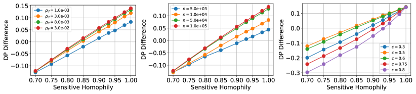
Figure 5: The difference of demographic parity for message passing with different initial covariance matrix. Left: DP difference for different graph connection density $\rho_{d}$ with senstive attribute ratio $c=0.5$ and number of nodes $n=10^{4}$; Middle: DP difference for different number of nodes $n$ with senstive attribute ratio $c=0.5$ and graph connection density $\rho_{d}=10^{-3}$; Right: DP difference for different senstive attribute ratio $c$ with graph connection density $\rho_{d}=10^{-3}$ and number of nodes $n=10^{4}$.

K.2 Hyperparameter Study

We provide hyperparameter study for further investigation on fairness and smoothness hyperparmeter on prediction and fairness performance on three datasets. Specifically, we tune hyperparameters as $\lambda_{f}=\{0.0,5.0,10.0,15.0,20.0,30.0,100.0,1000.0\}$ and $\lambda_{s}=\{0.0,0.1,0.5,1.0,3.0,5.0,10.0,15.0,20.0\}$. From the results in Figure 6, we can make the following observations:

• The accuracy and demographic parity are extremely sensitive to smoothness hyperparameter. It is seen that, for Pokec-n and Pokec-z datasets (NBA), larger smoothness hyperparameter usually leads to higher (lower) accuracy with higher prediction bias. The rationale is that, only for graph data with high label homophily coefficient, GCN-like aggregation with skip connection is beneficial. Otherwise, the neighbor’s node representation with different label will mislead representation update.

• The appropriate fairness hyperparameter leads to better fairness and prediction performance tradeoff. The reason is that fairness hyperparameter determinates the perturbation vector update step size in probability space. Only appropriate step size can lead to better perturbation vector update.

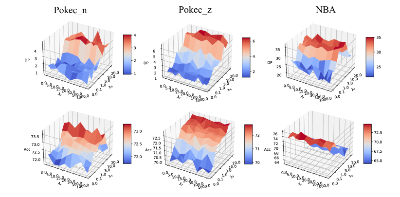
Figure 6: Hyperparameter study on fairness and smoothness hyperparameter for demographic parity and Accuracy.

K.3 Running Time Comparison

We provide running time comparison in Table 7 for our proposed FMP and other baselines, including vanilla, regularization and adversarial debiasing on many backbones (MLP, GCN, GAT, SGC, and APPNP). To achieve fair comparison, we adopt the same Adam optimizer with $200$ epochs with $5$ running times. We list several observations as follows:

• The running time of proposed FMP is very efficient for large-scale dataset. Specifically, for vanilla method, the running time of FMP is higher than most lighten backbone MLP with $46.97\%$ and $15.03\%$ time overhead on Pokec-n and Poken-z dataset, respectively. Compared with the most time-consumption APPNP, the running time of FMP is lower with $64.07\%$ and $41.45\%$ time overhead on Pokec-n and Poken-z dataset, respectively.

• The regularization method achieves almost the same running time compared with vanilla method on all backbones. For example, GCN with regularization encompasses higher running time with $6.41\%$ time overhead compared with vanilla method. Adversarial debiasing is extremely time-consuming. For example, GCN with adversarial debiasing encompasses higher running time with $88.58\%$ time overhead compared with vanilla method.

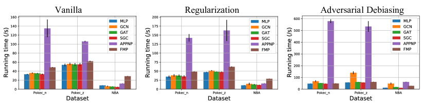
Figure 7: The running time comparison.

References

- Agarwal et al. (2021) Agarwal, C., Lakkaraju, H., and Zitnik, M. Towards a unified framework for fair and stable graph representation learning. arXiv preprint arXiv:2102.13186, 2021.
- Beutel et al. (2017) Beutel, A., Chen, J., Zhao, Z., and Chi, E. H. Data decisions and theoretical implications when adversarially learning fair representations. arXiv preprint arXiv:1707.00075, 2017.
- Bose & Hamilton (2019) Bose, A. and Hamilton, W. Compositional fairness constraints for graph embeddings. In International Conference on Machine Learning, pp. 715–724. PMLR, 2019.
- Bruna et al. (2013) Bruna, J., Zaremba, W., Szlam, A., and LeCun, Y. Spectral networks and locally connected networks on graphs. arXiv preprint arXiv:1312.6203, 2013.
- Buyl & De Bie (2020) Buyl, M. and De Bie, T. Debayes: a bayesian method for debiasing network embeddings. In International Conference on Machine Learning, pp. 1220–1229. PMLR, 2020.
- Chen et al. (2013) Chen, P., Huang, J., and Zhang, X. A primal–dual fixed point algorithm for convex separable minimization with applications to image restoration. Inverse Problems, 29(2):025011, 2013.
- Chien et al. (2021) Chien, E., Peng, J., Li, P., and Milenkovic, O. Adaptive universal generalized pagerank graph neural network. In International Conference on Learning Representations, 2021.
- Chuang & Mroueh (2020) Chuang, C.-Y. and Mroueh, Y. Fair mixup: Fairness via interpolation. In International Conference on Learning Representations, 2020.
- Creager et al. (2019) Creager, E., Madras, D., Jacobsen, J.-H., Weis, M., Swersky, K., Pitassi, T., and Zemel, R. Flexibly fair representation learning by disentanglement. In International conference on machine learning, pp. 1436–1445. PMLR, 2019.
- Dai & Wang (2021) Dai, E. and Wang, S. Say no to the discrimination: Learning fair graph neural networks with limited sensitive attribute information. In Proceedings of the 14th ACM International Conference on Web Search and Data Mining, pp. 680–688, 2021.
- Defferrard et al. (2016) Defferrard, M., Bresson, X., and Vandergheynst, P. Convolutional neural networks on graphs with fast localized spectral filtering. Advances in neural information processing systems, 29:3844–3852, 2016.
- Dong et al. (2016) Dong, Y., Lizardo, O., and Chawla, N. V. Do the young live in a “smaller world” than the old? age-specific degrees of separation in a large-scale mobile communication network. arXiv preprint arXiv:1606.07556, 2016.
- Du et al. (2021) Du, M., Mukherjee, S., Wang, G., Tang, R., Awadallah, A. H., and Hu, X. Fairness via representation neutralization. arXiv preprint arXiv:2106.12674, 2021.
- Feldman et al. (2015) Feldman, M., Friedler, S. A., Moeller, J., Scheidegger, C., and Venkatasubramanian, S. Certifying and removing disparate impact. In proceedings of the 21th ACM SIGKDD international conference on knowledge discovery and data mining, pp. 259–268, 2015.
- Fisher et al. (2020) Fisher, J., Mittal, A., Palfrey, D., and Christodoulopoulos, C. Debiasing knowledge graph embeddings. In Proceedings of the 2020 Conference on Empirical Methods in Natural Language Processing (EMNLP), pp. 7332–7345, 2020.
- Gao et al. (2018) Gao, H., Wang, Z., and Ji, S. Large-scale learnable graph convolutional networks. In Proceedings of the 24th ACM SIGKDD International Conference on Knowledge Discovery & Data Mining, pp. 1416–1424, 2018.
- Hamaguchi et al. (2017) Hamaguchi, T., Oiwa, H., Shimbo, M., and Matsumoto, Y. Knowledge transfer for out-of-knowledge-base entities: A graph neural network approach. arXiv preprint arXiv:1706.05674, 2017.
- Hamilton et al. (2017) Hamilton, W. L., Ying, R., and Leskovec, J. Inductive representation learning on large graphs. In Proceedings of the 31st International Conference on Neural Information Processing Systems, pp. 1025–1035, 2017.
- Henaff et al. (2015) Henaff, M., Bruna, J., and LeCun, Y. Deep convolutional networks on graph-structured data. arXiv preprint arXiv:1506.05163, 2015.
- Kipf & Welling (2017) Kipf, T. N. and Welling, M. Semi-supervised classification with graph convolutional networks. In International Conference on Learning Representations (ICLR), 2017.
- Klicpera et al. (2019) Klicpera, J., Bojchevski, A., and Günnemann, S. Predict then propagate: Graph neural networks meet personalized pagerank. In International Conference on Learning Representations, 2019.
- Köse & Shen (2021) Köse, Ö. D. and Shen, Y. Fairness-aware node representation learning. arXiv preprint arXiv:2106.05391, 2021.
- Kullback (1997) Kullback, S. Information theory and statistics. Courier Corporation, 1997.
- Laclau et al. (2021) Laclau, C., Redko, I., Choudhary, M., and Largeron, C. All of the fairness for edge prediction with optimal transport. In International Conference on Artificial Intelligence and Statistics, pp. 1774–1782. PMLR, 2021.
- Li et al. (2021) Li, P., Wang, Y., Zhao, H., Hong, P., and Liu, H. On dyadic fairness: Exploring and mitigating bias in graph connections. In International Conference on Learning Representations, 2021.
- Liu et al. (2021) Liu, X., Jin, W., Ma, Y., Li, Y., Liu, H., Wang, Y., Yan, M., and Tang, J. Elastic graph neural networks. In International Conference on Machine Learning, pp. 6837–6849. PMLR, 2021.
- Loris & Verhoeven (2011) Loris, I. and Verhoeven, C. On a generalization of the iterative soft-thresholding algorithm for the case of non-separable penalty. Inverse Problems, 27(12):125007, 2011.
- Louizos et al. (2015) Louizos, C., Swersky, K., Li, Y., Welling, M., and Zemel, R. The variational fair autoencoder. arXiv preprint arXiv:1511.00830, 2015.
- Louppe et al. (2017) Louppe, G., Kagan, M., and Cranmer, K. Learning to pivot with adversarial networks. In Proceedings of the 31st International Conference on Neural Information Processing Systems, pp. 982–991, 2017.
- Ma et al. (2021a) Ma, J., Deng, J., and Mei, Q. Subgroup generalization and fairness of graph neural networks. Advances in Neural Information Processing Systems, 34, 2021a.
- Ma et al. (2021b) Ma, Y., Liu, X., Shah, N., and Tang, J. Is homophily a necessity for graph neural networks? arXiv preprint arXiv:2106.06134, 2021b.
- Ma et al. (2021c) Ma, Y., Liu, X., Zhao, T., Liu, Y., Tang, J., and Shah, N. A unified view on graph neural networks as graph signal denoising. In Proceedings of the 30th ACM International Conference on Information & Knowledge Management, pp. 1202–1211, 2021c.
- Mehrabi et al. (2021) Mehrabi, N., Morstatter, F., Saxena, N., Lerman, K., and Galstyan, A. A survey on bias and fairness in machine learning. ACM Computing Surveys (CSUR), 54(6):1–35, 2021.
- Monti et al. (2017) Monti, F., Boscaini, D., Masci, J., Rodola, E., Svoboda, J., and Bronstein, M. M. Geometric deep learning on graphs and manifolds using mixture model cnns. In Proceedings of the IEEE conference on computer vision and pattern recognition, pp. 5115–5124, 2017.
- Rahman et al. (2019) Rahman, T., Surma, B., Backes, M., and Zhang, Y. Fairwalk: Towards fair graph embedding. 2019.
- Rockafellar (2015) Rockafellar, R. T. Convex analysis. Princeton university press, 2015.
- Suresh & Guttag (2019) Suresh, H. and Guttag, J. V. A framework for understanding unintended consequences of machine learning. arXiv preprint arXiv:1901.10002, 2, 2019.
- Takac & Zabovsky (2012) Takac, L. and Zabovsky, M. Data analysis in public social networks. In International scientific conference and international workshop present day trends of innovations, volume 1, 2012.
- Tang et al. (2020) Tang, X., Yao, H., Sun, Y., Wang, Y., Tang, J., Aggarwal, C., Mitra, P., and Wang, S. Investigating and mitigating degree-related biases in graph convoltuional networks. In Proceedings of the 29th ACM International Conference on Information & Knowledge Management, pp. 1435–1444, 2020.
- Veličković et al. (2018) Veličković, P., Cucurull, G., Casanova, A., Romero, A., Liò, P., and Bengio, Y. Graph attention networks. In International Conference on Learning Representations, 2018.
- Wu et al. (2019) Wu, F., Souza, A., Zhang, T., Fifty, C., Yu, T., and Weinberger, K. Simplifying graph convolutional networks. In International conference on machine learning, pp. 6861–6871. PMLR, 2019.
- Ying et al. (2018) Ying, R., He, R., Chen, K., Eksombatchai, P., Hamilton, W. L., and Leskovec, J. Graph convolutional neural networks for web-scale recommender systems. In Proceedings of the 24th ACM SIGKDD International Conference on Knowledge Discovery & Data Mining, pp. 974–983, 2018.
- Yurochkin & Sun (2020) Yurochkin, M. and Sun, Y. Sensei: Sensitive set invariance for enforcing individual fairness. In International Conference on Learning Representations, 2020.
- Zhang et al. (2018) Zhang, B. H., Lemoine, B., and Mitchell, M. Mitigating unwanted biases with adversarial learning. In Proceedings of the 2018 AAAI/ACM Conference on AI, Ethics, and Society, pp. 335–340, 2018.
- Zhao & Akoglu (2019) Zhao, L. and Akoglu, L. Pairnorm: Tackling oversmoothing in gnns. arXiv preprint arXiv:1909.12223, 2019.
- Zhu et al. (2020) Zhu, J., Yan, Y., Zhao, L., Heimann, M., Akoglu, L., and Koutra, D. Beyond homophily in graph neural networks: Current limitations and effective designs. Advances in neural information processing systems, 2020.
- Zhu et al. (2021) Zhu, M., Wang, X., Shi, C., Ji, H., and Cui, P. Interpreting and unifying graph neural networks with an optimization framework. In Proceedings of the Web Conference 2021, pp. 1215–1226, 2021.