Dynamic Heterogeneous Distribution Regression Panel Models, with an Application to Labor Income Processes^∗

Abstract.

We consider the estimation of a dynamic distribution regression panel data model with heterogeneous coefficients across units. The objects of primary interest are specific functionals of these coefficients. These include predicted actual and stationary distributions of the outcome variable and quantile treatment effects. Coefficients and their functionals are estimated via fixed effect methods. We investigate how these functionals vary in response to changes in initial conditions or covariate values. We also identify a uniformity issue related to the robustness of inference to the unknown degree of heterogeneity, and propose a cross-sectional bootstrap method for uniformly valid inference on function-valued objects. Employing PSID annual labor income data we illustrate some important empirical issues we can address. We first quantify the impact of a negative labor income shock on the distribution of future labor income. We also examine the impact on the distribution of labor income from increasing the education level of a chosen group of workers. Finally, we demonstrate the existence of heterogeneity in income mobility, and how this leads to substantial variation in individuals’ incidences to be trapped in poverty. We also provide simulation evidence confirming that our procedures work well.

Keywords: distribution regression, individual heterogeneity, panel data, uniform inference, labor income dynamics, incidental parameter problem, poverty traps

1. Introduction

Empirical studies increasingly feature analyses of data comprising repeated observations on the same or similar units. While the most common example is panel data, many of its attractive features are found in other data structures, such as network and spatial data. From an econometric perspective, the availability of panel data accommodates a treatment of time invariant unit-specific heterogeneity (see, for example, Mundlak 1978) and also provides internal instruments in the presence of time varying endogeneity (see, for example, Hausman and Taylor 1981, Arellano and Bond 1991). It also facilitates the estimation of dynamic relationships within unit, or contemporaneous relationships between units. However, a feature of the panel data literature is its limited treatment of parameter heterogeneity. Although the random coefficient panel model allows heterogeneous coefficients between units, and some recent developments that we discuss below incorporate heterogeneous coefficients within units, there are relatively few studies that incorporate heterogeneous coefficients both between and within units. Allowing both forms of heterogeneity is potentially important in many economic settings.

This paper employs random coefficient dynamic distribution regression to estimate a panel model with coefficient heterogeneity between and within units. The model captures within unit heterogeneous relationships between outcome and covariates through function-valued coefficients, and between unit heterogeneity via coefficients which can vary across units in an unrestricted fashion. The objects of interest are functionals of the coefficients including linear projections on individual covariates and predicted distributions. We consider the impact on these objects from manipulating the values of the initial conditions of the outcome or the covariates. We also consider both one-period-ahead and stationary counterfactual distributions to measure the short and long term effects of these changes.

Our proposed estimator employs fixed effect methods, which allow an unrestricted relationship between the unobserved unit-specific heterogeneity, the covariates, and the initial conditions. Estimation and inference consists of three steps. First, we estimate unit-specific coefficients by distribution regression exploiting the time series dimension of the panel. Second, we estimate the functionals of interest. We debias the estimates to account for the incidental parameter problem (Neyman and Scott, 1948). Third, we perform inference using a cross-sectional bootstrap method which resamples with replacement the estimated coefficients of the units noting that this avoids repeating the computationally expensive first-step estimation. We show how to construct confidence bands and test hypotheses for the quantiles and quantile effects, which are uniformly valid over a prespecified region of quantile indexes.

Our methodology is applicable to a wide range of settings and we employ it here to examine labor income dynamics. This is an important research area with a large literature, starting with Champernowne (1953), Hart (1976), Shorrocks (1976) and Lillard and Willis (1978), but now also including a long list of papers featuring econometric innovations. We apply our model to the Panel Study of Income Dynamics (PSID) data to perform experiments corresponding to various counterfactual analyses which cannot be conducted via existing methodologies.

First, we consider how a reduction in annual labor income in a given year, implemented via a negative shock, affects future annual labor income. We find that the predicted effect on the cross-sectional distribution of labor income after one period varies substantially after we account for heterogeneity in the level and persistence of income. Our model predicts substantially smaller effects than models that impose homogeneous effects.

Second, we examine the impact of increasing the education level of certain workers. While the effect of education on earnings is typically evaluated by its impact on the level of earnings, we explore how it may also operate through individual-specific income persistence. We also examine if it varies across quantiles of the income distribution. We investigate a hypothetical scenario that assigns 12 years of schooling to individuals who have not completed high school. We find important short and long run distributional effects as it increases the incomes of those in the lower tails of the one-period ahead and stationary labor income distributions. However, it has little effect on their upper tails. This exercise, which cannot be analyzed using traditional homogeneous autoregressive models, illustrates the importance of individual characteristics in determining the nature of earnings dynamics.

Finally, we address the existence of poverty traps. We explicitly model the heterogeneous conditional probabilities of individuals being in poverty in a specific year given they were in poverty in the previous year. We uncover substantial cross-sectional heterogeneity in the level and persistence of annual labor income and identify the responsible individual characteristics. This heterogeneity is shown to have implications for an individual’s tendency to remain below or above specific quantiles of the income distribution.

1.1. Relationship with existing literature

From a theoretical perspective, our paper is closest to Chernozhukov et al. (2013) (CFM) and Chernozhukov et al. (2018a) (CFW). The former studies distribution regression of cross-sectional data and the latter panel data with fixed effects. Both flexibly model and estimate counterfactual distributions. We introduce two substantial and important departures from this earlier work. First, whereas all coefficients in CFM and CFW (except the intercept) are fixed, we treat all coefficients as random. This enhances the model’s flexibility and facilitates the analysis of many economically interesting functionals which cannot be analyzed in the CFM and CFW frameworks. Moreover, our evidence below indicates they are empirically important. It also introduces the theoretical challenge of how to perform inference that remains uniformly valid with respect to the degree of heterogeneity in the coefficients. These issues have not been previously considered. Second, our model is dynamic, whereas the CFM and CFW models are static. This allows us to estimate economically interesting objects related to persistence.

Our model differs from the traditional random coefficients model of Swamy (1970), Hsiao and Pesaran (2008), Arellano and Bonhomme (2012), Fernández-Val and Lee (2013) and Su et al. (2016), among others, as we allow for heterogeneous coefficients both between and within units. It is more flexible than existing distribution and quantile regression models with fixed effects that allow the intercepts to vary across units but restrict the slopes to be homogeneous. See, for example, Koenker (2004), Galvao (2011), Galvao and Kato (2016), Kato et al. (2012), Arellano and Weidner (2017), and Chernozhukov et al. (2018a). Chetverikov et al. (2016), Okui and Yanagi (2019), Zhang et al. (2019) and Chen (2021) considered panel models with within and between unit heterogeneity. Okui and Yanagi (2019) provided methods to estimate distributions of heterogeneous moments such as means, autocovariances and autocorrelations. Their model and the objects they consider are different from ours. Zhang et al. (2019) proposed a quantile regression grouped panel data model with heterogeneous coefficients, but where the distribution of the coefficients is restricted to have finite support. Chetverikov et al. (2016) and Chen (2021) develop models similar to ours. They targeted projections of the model coefficients as the objects of interest, but did not consider counterfactual distributions. Chetverikov et al. (2016), Zhang et al. (2019) and Chen (2021) focused on models with strictly exogenous covariates, which exclude dynamic models that include lagged outcomes as covariates. Moreover, their methodology is based on quantile regression. Distribution regression has several appealing features in our setting including: (i) It deals with continuous, discrete and mixed outcomes without modification, and (ii) it yields simple analytical forms for the functionals of interest. In this sense, we extend the use of the distribution regression of Foresi and Peracchi (1995) to panel models with random coefficients.

Bias correction methods based on large-$T$ asymptotic approximations for fixed effects estimators of dynamic and nonlinear panel models were studied in Nickell (1981), Phillips and Moon (1999), Hahn and Newey (2004), Fernández-Val (2009), Hahn and Kuersteiner (2011), Dhaene and Jochmans (2015), and Fernández-Val and Weidner (2016), among others (see Arellano and Hahn (2007) and Fernández-Val and Weidner (2018) for recent reviews). We extend these debiasing methods to functionals of the coefficients. Inference that is robust to unknown heterogeneity has also been studied recently by Liao and Yang (2018) and Lu and Su (2022) in the context of linear panel models. The cross-sectional bootstrap was previously used for panel data as a resampling scheme that preserves the dependence in the time series dimension, e.g., Kapetanios (2008), Kaffo (2014), and Gonçalves and Kaffo (2015). We demonstrate that it also has robustness properties in models with heterogeneous coefficients.

Our approach is also novel from an empirical perspective although it is related to existing work. The literature examining labor income processes has typically focused on allocating the total error variances into transitory and permanent components. A summary is provided in Moffitt and Zhang (2018) and two important recent innovations are Arellano et al. (2017) and Hu et al. (2019). The first examined nonlinear persistence in the permanent component and how it varies over the earnings distribution. The second allowed for a flexible representation of the distributions of both components. Our approach is not intended to supersede these methodologies. Rather, we examine earnings dynamics to illustrate how we can complement these earlier studies. However, the approach most similar to ours is Arellano et al. (2017). While that paper also focused on the impact of earnings on consumption, an important feature is the treatment of the persistence in the earnings process. They considered a dynamic earnings process with nonlinear persistence that can vary by location in the earnings distribution. While our approach does not nest the models above, it does incorporate a generalized linear process which not only varies by location in the earnings distribution but also across workers. This cannot be accommodated by existing approaches. Moreover, we allow persistence to be a function of both observed and unobserved individual characteristics. Our analysis of income mobility and persistence relies on a representation of the model as a finite-state Markov chain when labor income is treated as discrete. Champernowne (1953) and Shorrocks (1976) previously used Markov chain representations of the labor income process to analyze the same issue. We allow unrestricted heterogeneity across workers by estimating a separate Markov chain for each worker. Finally, Hirano (2002) and Gu and Koenker (2017) estimated autoregressive labor income processes using flexible semiparametric Bayesian methods.

1.2. Main contributions

The paper makes three main contributions. First, we consider a model with heterogeneous function-valued coefficients. The heterogeneity between and within the coefficient functions makes the model very flexible and facilitates the analysis of various new functionals. Second, extending to a “flexible heterogeneous-coefficient” model is not straightforward. We provide an inference procedure which is valid uniformly over the degree of heterogeneity of the coefficients. The challenge in doing so is the unknown degree of heterogeneity in the coefficient functions, which allows homogeneous models as a special case. This affects both the rate of convergence and the asymptotic distribution of the fixed-effect estimators. This problem is further complicated since the degree of heterogeneity can vary continuously across different points of the coefficient function. We show that standard analytical plug-in methods do not provide valid inference in this setting. More formally, we establish that they break down in data generating processes where there is coefficient homogeneity or, more broadly, when the degree of heterogeneity is sufficiently small relative to the sample size at some point. To address this issue, we propose a cross-sectional bootstrap scheme that resamples from the empirical distribution of estimated heterogeneous random coefficients. We show that the bootstrap is valid uniformly over various degrees of heterogeneity. Third, we establish a connection between dynamic distribution regression models with discrete outcomes and finite-state Markov chains. This relationship is potentially very useful as it allows objects such as stationary distributions, mobility probabilities and recurrence times to be expressed as functionals of the coefficient functions.

1.3. Outline

The rest of the paper is organized as follows. Section 2 presents the model and objects of interest. Section 3 discusses estimation and inference. We present the empirical application in Section 4 and Section 5 establishes our associated asymptotic theory. for our estimation and inference methods. Section 6 reports simulation evidence. Proofs and additional results are gathered in the Appendix.

2. The model and objects of interest

2.1. The model

We observe a panel data set $\{(y_{it},\boldsymbol{x}_{it}):1\leq i\leq N,1\leq t\leq T\}$, where $i$ typically indexes observational units and $t$ time periods. The scalar variable $y_{it}$ represents the outcome or response of interest, which can be continuous, discrete or mixed; and $\boldsymbol{x}_{it}$ is a $d_{x}$-vector of covariates, which includes a constant, lagged outcome values, and other predetermined covariates denoted by $\boldsymbol{v}_{it}$, that is

$$\boldsymbol{x}_{it}=(1,y_{i(t-1)},...,y_{i(t-L)},\boldsymbol{v}_{it}^{\prime})^{\prime}.$$

Let $\mathcal{F}_{it}$ be a filtration over $t$ that includes $\boldsymbol{x}_{it}$ and any time invariant variable for unit $i$. We model the distribution of $y_{it}$ conditional on $\mathcal{F}_{it}$ as, for any $y\in\mathbb{R}$,

$$\Pr(y_{it}\leq y\mid\mathcal{F}_{it})=\Lambda(-\boldsymbol{x}_{it}^{\prime}\boldsymbol{\beta}_{i}(y)),\quad 1\leq t\leq T,\quad 1\leq i\leq N,$$ (2.1)

where $\Lambda:\mathbb{R}\mapsto[0,1]$ is a known, strictly increasing link function (e.g., the standard normal or logistic distribution CDF), and $y\mapsto-\boldsymbol{x}_{it}^{\prime}\boldsymbol{\beta}_{i}(y)$ is increasing almost surely (a.s). This is a distribution regression model for panel data with heterogeneous coefficients which we call a heterogeneous distribution regression (HDR).

The model embodies a Markov-type condition for each individual as only the first $L$ lags of the outcome and contemporaneous values of the other covariates determine the conditional distribution of $y_{it}$. It imposes an index restriction on the effect of $\boldsymbol{x}_{it}$ although this restriction is mild as the coefficient $\boldsymbol{\beta}_{i}(y)$ varies with $i$ and $y$, and can be further weakened by replacing $\boldsymbol{x}_{it}$ by $P(\boldsymbol{x}_{it})$, where $P$ is a vector of transformations of $\boldsymbol{x}_{it}$. Our theory would still apply provided that $P$ is known and has fixed dimension.

By iterating expectations, the cross-sectional distribution of the observed outcome at time $t$ can be written in terms of the model coefficients as

$$F_{t}(y):=\mathbb{E}_{t}1\{y_{it}\leq y\}=\mathbb{E}_{t}\mathbb{E}(1\{y_{it}\leq y\}\mid\mathcal{F}_{it})=\mathbb{E}_{t}\Lambda(-\boldsymbol{x}_{it}^{\prime}\boldsymbol{\beta}_{i}(y)),$$ (2.2)

where the expectation $\mathbb{E}_{t}$ is taken with respect to the joint cross-sectional distribution of the variables in $\mathcal{F}_{it}$ at time $t$. This representation serves several purposes. First, it is the basis for a specification test of the model where an estimator of (2.2) is compared with the cross-sectional empirical distribution of $y_{it}$. Second, when $\boldsymbol{x}_{it}$ only includes lagged values of $y_{it}$, we can construct one-period-ahead predicted distributions by setting $t=T+1$. These distributions are useful for forecasting. Third, we can analyze dynamics of the distribution of $y_{it}$ over time. For example, below we analyze labor income mobility and the persistence of poverty traps. Fourth, we can consider the impact of interventions by comparing the counterfactual distribution after some intervention with the actual distribution.

2.2. Heterogeneous coefficient functions

The main innovation of (2.1) is all coefficients are random functions,

$$y\mapsto\boldsymbol{\beta}_{i}(y),$$

where the variations on $i$ and $y$ capture between-unit heterogeneity and within-unit heterogeneity, respectively. Moreover, we can explore if the two sources of heterogeneity are associated with observed unit characteristics using linear projections. Let $\boldsymbol{w}_{i},\boldsymbol{z}_{i}\in\mathcal{F}_{i1}$ denote time invariant covariates such that $\dim(\boldsymbol{w}_{i})\geq\dim(\boldsymbol{z}_{i})$ and $\mathbb{E}(\boldsymbol{w}_{i}\boldsymbol{z}_{i}^{\prime})$ has full column rank. Consider the instrumental variable projection of $\boldsymbol{\beta}_{i}(y)$ on $\boldsymbol{z}_{i}$

$$\boldsymbol{\beta}_{i}(y)=\boldsymbol{\theta}(y)\boldsymbol{z}_{i}+\boldsymbol{\gamma}_{i}(y),\quad\mathbb{E}(\boldsymbol{\gamma}_{i}(y)\mid\boldsymbol{w}_{i})=0,$$ (2.3)

which covers the standard linear projection by setting $\boldsymbol{w}_{i}=\boldsymbol{z}_{i}$. This object examines which covariates are associated with the heterogeneity in $\boldsymbol{\beta}_{i}(y)$ across $i$, where we allow these associations to vary within the distribution as indexed by $y$.

It is important to allow for multiple degrees of between-unit heterogeneity in these projections. For now, suppose $\dim(\boldsymbol{\gamma}_{i}(y))=1$. The degree of between-unit heterogeneity is mainly governed by

$$\mathsf{Var}(\boldsymbol{\gamma}_{i}(y)|\boldsymbol{w}_{i})\in[0,C]$$

for some $C>0$. Being zero or nearly so makes $\boldsymbol{\beta}_{i}(y)$ mostly concentrated around its conditional mean value $\boldsymbol{\theta}(y)\boldsymbol{z}_{i}$, while a strictly positive $\mathsf{Var}(\boldsymbol{\gamma}_{i}(y)|\boldsymbol{w}_{i})$ makes these coefficients more dispersed across units. The strength of this variance is unknown and is allowed to vary across $y$. Therefore, our model is flexible with respect to the degree of cross-sectional heterogeneity at different quantile levels. $\mathsf{Var}(\boldsymbol{\gamma}_{i}(y)|\boldsymbol{w}_{i})$ changing across $y$ reflects the covariates $\boldsymbol{z}_{i}$ different capacity to explain $\boldsymbol{\beta}_{i}(y)$ at different quantiles. Our empirical application explores whether initial income, education, race and year of birth are associated with differences in the level and persistence of labor income at different locations of the income distribution.

2.3. Counterfactual distributions

Our model can be used to construct flexible counterfactual distributions resulting from changing the covariates and the coefficients

$$G_{t}(y)=\mathbb{E}_{t}\Lambda(-h_{it}(\boldsymbol{x}_{it})^{\prime}\boldsymbol{\beta}^{g}_{i}(y)),$$ (2.4)

where $h_{it}$ is a possibly data dependent transformation, and $\boldsymbol{\beta}_{i}^{g}(y)$ is a transformation of the random coefficients. Specifically, we consider

$$\boldsymbol{\beta}_{i}^{g}(y)=\boldsymbol{\theta}(y)g(\boldsymbol{z}_{i})+\boldsymbol{\gamma}_{i}(y)=\boldsymbol{\beta}_{i}(y)+\boldsymbol{\theta}(y)[g(\boldsymbol{z}_{i})-\boldsymbol{z}_{i}],$$

for a known transformation $g$ of the time invariant covariates $\boldsymbol{z}_{i}$. This transformation allows us to study the effect of changing covariates on the cross-sectional distribution through their impact on the random coefficients.

For instance, consider a hypothetical scenario where at time $t$ we increase the number of years of schooling to 12 for any worker who has less. If $\boldsymbol{z}_{i}=(z_{1i},\boldsymbol{z}_{-1,i}^{\prime})^{\prime}$, where $z_{1i}$ is the observed years of schooling of worker $i$ and $\boldsymbol{z}_{-1,i}$ includes the remaining components of $\boldsymbol{z}_{i}$, this counterfactual scenario is implemented via the transformation

$$g(\boldsymbol{z}_{i})=(\max(z_{1i},12),\boldsymbol{z}_{-1,i}).$$ (2.5)

$G_{t}(y)$ would then represent the counterfactual distribution of labor income at $t$ after the change. Another example is

$$g(\boldsymbol{z}_{i})=(z_{1i}+1,\boldsymbol{z}_{-1,i}),$$

which corresponds to giving an additional year of schooling to all workers.

We can also study the impact of shocks in dynamic models. For example, suppose at time $t-1$ a shock reduces income by $100*\kappa\%$ for individuals with income higher than certain (known) threshold $\tau_{0}$. This corresponds to the transformation

$$h_{it}(\boldsymbol{x}_{it})=(1,y_{i(t-1)}+1\{y_{i(t-1)}>\log\tau_{0}\}\log(1-\kappa))^{\prime},$$ (2.6)

where $y_{i(t-1)}$ is measured in logarithmic scale. $G_{t}(y)$ now represents the counterfactual income distribution resulting from this income shock at time $t$.

2.4. Other objects of interest

2.4.1. Stationary distributions:

Assume the process $\{y_{i1},\ldots,y_{iT}\}$ is ergodic for each $i$, $y_{it}$ is discrete with support $\mathcal{Y}_{i}=\{y_{i}^{1}<\cdots<y_{i}^{K}\}$, which might be different for each unit, and the only covariate is the first lag of the outcome, i.e. $\boldsymbol{x}_{it}=(1,y_{i(t-1)})^{\prime}$. The conditional distribution can now be represented by a time-homogeneous $K$-state Markov chain and the stationary distribution can be characterized from the transition matrix of the Markov chain. This can be extended to include additional lags of the outcome variable at the cost of more cumbersome notation.

For each $i$, let $\boldsymbol{P}_{i}$ be the $K\times K$ transition matrix. The typical element of this matrix can be expressed as

$$P_{i,jk}=\Pr(y_{it}=y_{i}^{j}\mid y_{i(t-1)}=y_{i}^{k},\mathcal{F}_{it})=\Lambda\left(-\boldsymbol{x}_{i}^{k^{\prime}}\boldsymbol{\beta}_{i}(y_{i}^{j})\right)-1(j>1)\Lambda\left(-\boldsymbol{x}_{i}^{k^{\prime}}\boldsymbol{\beta}_{i}(y_{i}^{j-1})\right),$$ (2.7)

where $\boldsymbol{x}_{i}^{k}=(1,y_{i}^{k})^{\prime}$. By standard theory for Markov Chains, see, e.g., (Hamilton, 2020, p. 684), the ergodic probabilities $\boldsymbol{\pi}_{i}=(\pi_{i1},\ldots,\pi_{iK})$ are

$$\boldsymbol{\pi}_{i}=(\boldsymbol{A}_{i}^{\prime}\boldsymbol{A}_{i})^{-1}\boldsymbol{A}_{i}^{\prime}\boldsymbol{e}_{K+1},\quad\boldsymbol{A}_{i}=\left(\begin{array}[]{c}\boldsymbol{I}_{K}-\boldsymbol{P}_{i}\\ \boldsymbol{1}^{\prime}\end{array}\right),$$

where $\boldsymbol{I}_{K}$ is the identity matrix of size $K$, $\boldsymbol{1}$ is a $K$-vector of ones, and $\boldsymbol{e}_{K+1}$ is the $(K+1)$th column of $\boldsymbol{I}_{K+1}$. The cross-sectional stationary actual distribution is now

$$F_{\infty}(y)=\mathbb{E}[F_{i,\infty}(y)],\quad F_{i,\infty}(y)=\sum_{k:y_{i}^{k}\leq y}\pi_{ik},$$

where $F_{i,\infty}$ is a step function with steps at the elements of $\mathcal{Y}_{i}$.

Stationary counterfactual distributions can be formed by replacing $\boldsymbol{\beta}_{i}(y_{i}^{j})$ by $\boldsymbol{\beta}_{i}^{g}(y_{i}^{j})$ in (2.7). That is

$$P^{g}_{i,jk}=\Lambda\left(-\boldsymbol{x}_{i}^{k^{\prime}}\boldsymbol{\beta}^{g}_{i}(y_{i}^{j})\right)-1(j>1)\Lambda\left(-\boldsymbol{x}_{i}^{k^{\prime}}\boldsymbol{\beta}^{g}_{i}(y_{i}^{j-1})\right).$$

We denote the resulting cross-sectional stationary distribution as $G_{\infty}$. We do not consider transformations $h_{it}$ as they would produce the stationary distribution $F_{\infty}$. Note that changes in $y_{i(t-1)}$ do not affect the stationary distribution by the ergodicity assumption. The stationary distribution is useful for analyzing dynamics of the distribution of $y_{it}$ in the long run. We employ it below to examine labor income mobility and the persistence of poverty traps.

2.4.2. Quantile effects

We consider quantiles of the actual and counterfactual cross-sectional distributions, and define quantile effects as their difference. Given a univariate distribution $F$, the quantile (left-inverse) operator is

$$\phi(F,\tau):=\inf\{y\in\mathbb{R}:F(y)\geq\tau\},\quad\tau\in[0,1].$$

We apply this operator to the cross-sectional distributions defined above to obtain the quantile effects as

$$\mathsf{QE}_{t}(\tau):=\phi(G_{t},\tau)-\phi(F_{t},\tau),\quad\mathsf{QE}_{\infty}(\tau):=\phi(G_{\infty},\tau)-\phi(F_{\infty},\tau),\quad\tau\in[0,1].$$

These quantile effects measure the short and long term impacts of the hypothetical policies at different parts of the outcome distribution. They are unconditional or marginal as they are based on comparisons between counterfactual and actual marginal distributions.

3. Estimation and Inference Methods

3.1. Estimators

We employ a two-step procedure in which the first step obtains the model coefficients and the second constructs the desired functionals. When quantile effects are of interest we obtain them via a additional step.

The coefficients are estimated by HDR applied separately to the time series dimension of each unit, with debiasing to address the incidental parameter problem. The functionals of the coefficients are estimated using the plug-in method. The estimators of the distributions are debiased. The estimators of the projection coefficients do not need to be debiased as they are linear functionals of the coefficients. The quantile effects are estimated by applying the generalized inverse operator of Chernozhukov et al. (2010).

3.1.1. First stage: Model coefficients

We start with the DR estimator of $\boldsymbol{\beta}_{i}(y)$. That is

$$\widetilde{\boldsymbol{\beta}}_{i}(y)=\arg\max_{\beta\in\mathbb{R}^{d_{x}}}Q_{y,i}(\beta),\quad y\in\mathcal{Y}_{i},\quad i=1,...,N,$$

where

$$Q_{y,i}(\beta)=\sum_{t=1}^{T}1\{y_{it}\leq y\}\log\Lambda(-\boldsymbol{x}_{it}^{\prime}\beta)+\sum_{t=1}^{T}1\{y_{it}>y\}\log[1-\Lambda(-\boldsymbol{x}_{it}^{\prime}\beta)],$$

and $\mathcal{Y}_{i}$ is the set of observed values of the outcome for unit $i$, i.e. $\mathcal{Y}_{i}=\{y_{i1},\ldots,y_{iT}\}$. If $\Lambda$ is the standard normal or logistic link, these are standard logit or probit estimators. We then obtain $\widetilde{\boldsymbol{\beta}}_{i}(y)$ for other values of $y$ noting that $y\mapsto\widetilde{\boldsymbol{\beta}}_{i}(y)$ is a vector of step functions with steps at the elements of $\mathcal{Y}_{i}$.

Two complications arise: $\widetilde{\boldsymbol{\beta}}_{i}(y)$ is well-defined only if $y\in[\underline{y}_{i},\overline{y}_{i})$, where $\underline{y}_{i}=\min_{1\leq t\leq T}y_{it}$ and $\overline{y}_{i}=\max_{1\leq t\leq T}y_{it}$, and, when $\widetilde{\boldsymbol{\beta}}_{i}(y)$ is well-defined, it has bias of order $O(T^{-1})$. Let $N_{0}(y)$ be the number of indexes $i$ for which $y<\underline{y}_{i}$, $N_{1}(y)$ be the number of indexes $i$ for which $y\geq\overline{y}_{i}$, and $N_{01}(y)=N-N_{0}(y)-N_{1}(y)$ denote the number of indexes $i$ for which $\widetilde{\boldsymbol{\beta}}_{i}(y)$ exists. Without loss of generality we rearrange the index $i$ such that $\widetilde{\boldsymbol{\beta}}_{i}(y)$ exists for all $i=1,\ldots,N_{01}(y)$. We show below how to adjust the plug-in estimators of the functionals to incorporate the units $i>N_{01}(y)$.

Due to the incidental parameter bias it is necessary to debias $\widetilde{\boldsymbol{\beta}}_{i}(y)$ when $T$ is of moderate size relative to $N$. Plug-in estimators of nonlinear functionals based on debiased estimators are easier to debias than those based on the initial estimators. We debias $\widetilde{\boldsymbol{\beta}}_{i}(y)$ using analytical methods. That is

$$\widehat{\boldsymbol{\beta}}_{i}(y)=\widetilde{\boldsymbol{\beta}}_{i}(y)-\frac{\widehat{B}_{i,T}(y)}{T},\quad i=1,\ldots,N_{01}(y),$$ (3.1)

where $\widehat{B}_{i,T}(y)$ is a consistent estimator of the bias of $\widetilde{\boldsymbol{\beta}}_{i}(y)$ of order $O(T^{-1})$. The specific expressions of the bias and its estimator are presented in the Appendix, where we also consider alternative debiasing methods based on Jackknife (Dhaene and Jochmans, 2015). While our theory applies to both analytical and Jackknife methods, we focus on analytical methods because they have less demanding data requirements and performed better in our numerical simulations.

3.1.2. Second stage: Functionals

We provide estimators for all the functionals of interest. Denote the second derivative of the link function by $\ddot{\Lambda}$.

Projections of coefficients

A plug-in estimator of $\boldsymbol{\theta}(y)$ corresponds to applying two-stage least squares to (2.3) replacing $\boldsymbol{\beta}_{i}(y)$ by $\widehat{\boldsymbol{\beta}}_{i}(y)$. This yields,

$$\widehat{\boldsymbol{\theta}}(y)=\sum_{i=1}^{N_{01}(y)}\widehat{\boldsymbol{\beta}}_{i}(y)\widehat{\boldsymbol{z}}_{i}(y)^{\prime}\left(\sum_{i=1}^{N_{01}(y)}\widehat{\boldsymbol{z}}_{i}(y)\widehat{\boldsymbol{z}}_{i}(y)^{\prime}\right)^{-1},$$ (3.2)

where

$$\widehat{\boldsymbol{z}}_{i}(y):=\sum_{j=1}^{N_{01}(y)}z_{j}\boldsymbol{w}_{j}^{\prime}\left(\sum_{j=1}^{N_{01}(y)}\boldsymbol{w}_{j}\boldsymbol{w}_{j}^{\prime}\right)^{-1}\boldsymbol{w}_{i}.$$

When $\boldsymbol{w}_{i}=\boldsymbol{z}_{i}$, the estimator simplifies to the OLS estimator with $\widehat{\boldsymbol{z}}_{i}(y)=\boldsymbol{z}_{i}$.

Actual and counterfactual distributions

The plug-in estimators of the actual and counterfactual distributions are

$$\widehat{F}_{t}(y) = \frac{1}{N}\sum_{i=1}^{N_{01}(y)}\Lambda(-\boldsymbol{x}_{it}^{\prime}\widehat{\boldsymbol{\beta}}_{i}(y))+\frac{N_{1}(y)}{N}-\frac{\widehat{B}(y)}{T},$$ (3.3)

$$\widehat{G}_{t}(y) = \frac{1}{N}\sum_{i=1}^{N_{01}(y)}\Lambda(-h(\boldsymbol{x}_{it})^{\prime}\widehat{\boldsymbol{\beta}}^{g}_{i}(y))+\frac{N_{1}(y)}{N}-\frac{\widehat{B}_{G}(y)}{T},$$ (3.4)

where

$$\widehat{\boldsymbol{\beta}}_{i}^{g}(y) = \widehat{\boldsymbol{\beta}}_{i}(y)+\widehat{\boldsymbol{\theta}}(y)[g(\boldsymbol{z}_{i})-\boldsymbol{z}_{i}],$$

$$\widehat{B}(y) = \frac{1}{2}\frac{1}{N}\sum_{i=1}^{N_{01}(y)}\mathsf{tr}\left(\ddot{\Lambda}(-\boldsymbol{x}_{it}^{\prime}\widehat{\boldsymbol{\beta}}_{i}(y))\boldsymbol{x}_{it}\boldsymbol{x}_{it}^{\prime}\widehat{\Sigma}_{i}(y)^{-1}\right)$$

$$\widehat{B}_{G}(y) = \frac{1}{2}\frac{1}{N}\sum_{i=1}^{N_{01}(y)}\mathsf{tr}\left(\ddot{\Lambda}(-h(\boldsymbol{x}_{it})^{\prime}\widehat{\boldsymbol{\beta}}^{g}_{i}(y))h(\boldsymbol{x}_{it})h(\boldsymbol{x}_{it})^{\prime}\widehat{\Sigma}_{i}(y)^{-1}\right).$$

Here $\widehat{B}(y)$ and $\widehat{B}_{G}(y)$ are estimators of the first-order bias coming from the nonlinearity of $F_{t}$ and $G_{t}$ as a functional of $\boldsymbol{\beta}(y)$, and $\widehat{\Sigma}_{i}(y)^{-1}$ is an estimator of the asymptotic variance-covariance matrix of $\sqrt{T}(\widetilde{\boldsymbol{\beta}}_{i}(y)-\boldsymbol{\beta}_{i}(y))$. For units for which $\widehat{\boldsymbol{\beta}}_{i}(y)$ is not well-defined we set $\Lambda(-\boldsymbol{x}_{it}^{\prime}\boldsymbol{\beta}_{i}(y))=\Lambda(-h(\boldsymbol{x}_{it})^{\prime}\boldsymbol{\beta}^{g}_{i}(y))=1$ if $y<\underline{y}_{i}$ and $\Lambda(-\boldsymbol{x}_{it}^{\prime}\boldsymbol{\beta}_{i}(y))=\Lambda(-h(\boldsymbol{x}_{it})^{\prime}\boldsymbol{\beta}^{g}_{i}(y))=0$ if $y\geq\overline{y}_{i}$.

Stationary distributions

We start with the empirical transition matrix as a preliminary plug-in estimator of $\boldsymbol{P}_{i}$, which we modify to enforce that all entries are non-negative and the rows add to one. More precisely, we define the $K\times K$ matrix $\widehat{\boldsymbol{Q}}_{i}$ with typical element

$$\widehat{Q}_{i,jk}=1(j=K)+1(j<K)\Lambda\left(-\boldsymbol{x}_{i}^{k^{\prime}}\widehat{\beta}_{i}(y_{i}^{j})\right).$$ (3.5)

For each row of $\widehat{\boldsymbol{Q}}_{i}$, we sort (rearrange) the elements in increasing order to form the matrix $\check{\boldsymbol{Q}}_{i}$ with typical element $\check{Q}_{i,jk}$. We then construct the empirical transition matrix $\widehat{\boldsymbol{P}}_{i}$ with typical element

$$\widehat{P}_{i,jk}=\check{Q}_{i,jk}-1(j>1)\check{Q}_{i,(j-1)k}.$$

The empirical ergodic probabilities $\widehat{\boldsymbol{\pi}}_{i}=(\widehat{\pi}_{i1},\ldots,\widehat{\pi}_{iK})$ are now

$$\widehat{\boldsymbol{\pi}}_{i}=(\widehat{\boldsymbol{A}}_{i}^{\prime}\widehat{\boldsymbol{A}}_{i})^{-1}\widehat{\boldsymbol{A}}_{i}^{\prime}\boldsymbol{e}_{K+1}-\frac{1}{T}\widehat{B}_{\boldsymbol{\pi}_{i}},\quad\widehat{\boldsymbol{A}}_{i}=\left(\begin{array}[]{c}\boldsymbol{I}_{K}-\widehat{\boldsymbol{P}}_{i}\\ \boldsymbol{1}^{\prime}\end{array}\right),$$

where $\widehat{B}_{\boldsymbol{\pi}_{i}}$ is an estimator of the bias coming from the nonlinearity of $\boldsymbol{\pi}_{i}$ as a functional of $(\boldsymbol{\beta}_{i}(y_{i}^{1}),\ldots,\boldsymbol{\beta}_{i}(y_{i}^{K}))$. We give the expression of $\widehat{B}_{\boldsymbol{\pi}_{i}}$ in the Appendix.

The estimator of the stationary distribution is

$$\widehat{F}_{\infty}(y)=\frac{1}{N}\sum_{i=1}^{N}\widehat{F}_{i,\infty}(y),\quad\widehat{F}_{i,\infty}(y)=\sum_{k:y_{i}^{k}\leq y}\widehat{\pi}_{ik}.$$

Estimators of stationary counterfactual distributions can be formed by replacing $\widehat{\boldsymbol{\beta}}_{i}(y_{i}^{j})$ by $\widehat{\boldsymbol{\beta}}_{i}^{g}(y_{i}^{j})$ and modifying the bias estimator, $\widehat{B}_{\boldsymbol{\pi}_{i}}$, in (3.3). The modified expression of the estimator of the bias is given in the Appendix. The resulting estimator of $G_{\infty}$ is denoted by $\widehat{G}_{\infty}$.

3.1.3. Quantile effects

The estimators of the quantile effects are:

$$\widehat{\mathsf{QE}}_{t}(\tau)=\widetilde{\phi}(\widehat{G}_{t},\tau)-\widetilde{\phi}(\widehat{F}_{t},\tau),$$ (3.6)

where $\widetilde{\phi}$ is the generalized inverse or rearrangement operator

$$\widetilde{\phi}(F,\tau)=\int_{0}^{\infty}1\{F(y)\leq\tau\}\mathrm{d}y-\int_{-\infty}^{0}1\{F(y)\geq\tau\}\mathrm{d}y$$

which monotonizes $y\mapsto F(y)$ before applying the inverse operator.

3.2. Inference

To begin we highlight an important problem with standard analytical plug-in methods where the heterogeneous coefficients are estimated via fixed effect approaches. We show that these methods are not uniformly valid with respect to the degree of heterogeneity as measured by the variance of the coefficients. We propose a cross-sectional bootstrap scheme that has good computational properties and in Section 5.4.1 we prove its uniform validity over a large class of data generating processes.

3.2.1. Inference problem

While the inference problem affects all the functionals we consider, we illustrate it via a simple example that abstracts from other complications such as the need to debias. Consider the model

$$y_{it}=\beta_{i}+e_{it},\quad\mathbb{E}(e_{it}\mid\beta_{i})=0,\quad\mathbb{E}(\beta_{i})=\theta,$$

where we allow $\mathsf{Var}(\beta_{i})\in[0,C]$ to be on a compact support, with zero as an admissible value. This class of data generating processes captures different degrees of heterogeneity that might arise in empirical applications. For simplicity, we assume $e_{it}$ and $\beta_{i}$ are both i.i.d. sequences in both $i$ and $t$ and mutually independent. The estimator of $\theta$ is

$$\widehat{\theta}=\frac{1}{N}\sum_{i=1}^{N}\widehat{\beta}_{i},\quad\widehat{\beta}_{i}=\frac{1}{T}\sum_{t=1}^{T}y_{it}=\beta_{i}+\frac{1}{T}\sum_{t=1}^{T}e_{it}.$$

The goal is to make inference about $\theta$ based on $\widehat{\theta}$ that remains uniformly valid over $\mathsf{Var}(\beta_{i})\in[0,C]$.

Let $\overline{\beta}=\sum_{i=1}^{N}\beta_{i}/N$. The asymptotic distribution of $\widehat{\theta}$ is determined by two components:

$$\widehat{\theta}-\theta=(\widehat{\theta}-\overline{\beta})+(\overline{\beta}-\theta),$$

where

$$\widehat{\theta}-\overline{\beta} = \frac{1}{NT}\sum_{i=1}^{N}\sum_{t=1}^{T}e_{it},\quad\overline{\beta}-\theta=\frac{1}{N}\sum_{i=1}^{N}(\beta_{i}-\mathbb{E}(\beta_{i})).$$

While both terms admit central limit theorems, they may have different rates of convergence. The rate of convergence of $\overline{\beta}-\theta$ depends on the degree of heterogeneity, $\mathsf{Var}(\beta_{i})$, which is unknown. We know that it is supported on a compact set $[0,C]$ for some $C>0$, with zero as an admissible boundary. This makes the final rate of convergence and the associated asymptotic distribution unknown. To illustrate this, consider two special extreme cases:

1. Strong heterogeneity: It is customary in the literature to assume that $\mathsf{Var}(\beta_{i})$ is bounded away from zero, such that $\overline{\beta}-\theta=O_{P}(N^{-1/2})$. Then this term dominates in the expansion, yielding

   $$\sqrt{N}(\widehat{\theta}-\theta)\to^{d}\mathcal{N}(0,\mathsf{Var}(\beta_{i})).$$

2. Weak heterogeneity: If $\mathsf{Var}(\beta_{i})$ is near the zero boundary, such that when treated as a sequence, it decays faster than $O(T^{-1})$, then $\widehat{\theta}-\overline{\beta}$ becomes the dominating term, yielding

   $$\sqrt{NT}(\widehat{\theta}-\theta)\to^{d}\mathcal{N}(0,\mathsf{Var}(e_{it})).$$

   We refer to this case as “weak heterogeneity” as it corresponds to a homogeneous $\beta_{i}$ or when the degree of heterogeneity is small relative to the sample size as formalized by $\mathsf{Var}(\beta_{i})=o(T^{-1})$. This may arise in empirical applications where the degree of heterogeneity is unknown and the time dimension is only moderately large.

It can be shown that any degree of heterogeneity between the above two extreme cases would lead to an unknown rate of convergence $\widehat{\theta}-\theta=O_{P}(\xi_{NT})$ where $\xi_{NT}\in[(NT)^{-1/2},N^{-1/2}]$. Moreover, this unknown rate of convergence has consequences for the properties of standard inferential methods. Note that

$$\mathsf{Var}(\widehat{\theta})=\frac{1}{NT}\mathsf{Var}(e_{it})+\frac{1}{N}\mathsf{Var}(\beta_{i}).$$ (3.7)

A common method to estimate this variance is to plug in sample analogs of $\mathsf{Var}(e_{it})$ and $\mathsf{Var}(\beta_{i})$. This procedure, however, does not provide uniformly valid inference. To illustrate the issue, consider the estimation of $\mathsf{Var}(\beta_{i})$. If $\beta_{i}$ were known, it could be estimated by

$$\widetilde{\mathsf{Var}}(\beta_{i}):=\frac{1}{N}\sum_{i=1}^{N}(\beta_{i}-\overline{\beta})^{2}.$$ (3.8)

Replacing $\beta_{i}$ with its consistent estimator $\widehat{\beta}_{i}$, we obtain

$$\widehat{\mathsf{Var}}(\beta_{i}):=\frac{1}{N}\sum_{i=1}^{N}(\widehat{\beta}_{i}-\widehat{\theta})^{2}.$$

Then $\widehat{\mathsf{Var}}(\beta_{i})-\mathsf{Var}(\beta_{i})$ has the following decomposition:

$$\underbrace{\frac{1}{N}\sum_{i=1}^{N}[(\widehat{\beta}_{i}-\widehat{\theta})^{2}-(\beta_{i}-\overline{\beta})^{2}]}_{\beta\text{- estimation error}}+\underbrace{\frac{1}{N}\sum_{i=1}^{N}[(\beta_{i}-\overline{\beta})^{2}-\mathsf{Var}(\beta_{i})]}_{\text{LLN- error}},$$ (3.9)

where “LLN- error” refers to the error associated with the law of large numbers.

The main issue is that the $\beta$- estimation error cannot be controlled uniformly over $\mathsf{Var}(\beta_{i})\in[0,C]$. Note that

$$\widehat{\beta}_{i}-\widehat{\theta}=\beta_{i}-\overline{\beta}+(\bar{e}_{i}-\bar{e}),\quad\bar{e}_{i}=\frac{1}{T}\sum_{t=1}^{T}e_{it},\quad\bar{e}=\frac{1}{N}\sum_{i=1}^{N}\bar{e}_{i}.$$

This, if $T=o(N)$, leads to

$$\beta\text{- estimation error}=\frac{1}{N}\sum_{i}(\bar{e}_{i}-\bar{e})^{2}+\frac{2}{N}\sum_{i}(\bar{e}_{i}-\bar{e})(\beta_{i}-\overline{\beta})\asymp O_{P}(T^{-1}).$$

The $\beta$-estimation error is an incidental parameter bias whose order does not adapt to $\mathsf{Var}(\beta_{i})$, leading to first order bias of $\widehat{\mathsf{Var}}(\widehat{\theta})$ in the weak heterogeneity case. Thus, the estimation error $|\widehat{\mathsf{Var}}(\widehat{\theta})-\mathsf{Var}(\widehat{\theta})|$ is lower bounded by an order of $O_{P}((NT)^{-1})$, which is not negligible when $\sqrt{NT}(\widehat{\theta}-\theta)\to^{d}\mathcal{N}(0,\mathsf{Var}(e_{it}))$. Consequently, the usual plug-in variance estimator using $\widehat{\mathsf{Var}}(\widehat{\theta})$ would lead to an asymptotically incorrect inference. To see this, note that the confidence interval will be distorted by a quantity of the same order as the length of the interval, that is

$$\mathsf{CI}_{1-p}(\theta)=\widehat{\theta}\pm z_{1-p/2}\sqrt{\widehat{\mathsf{Var}}(\widehat{\theta})}=\widehat{\theta}\pm z_{1-p/2}\sqrt{\mathsf{Var}(\widehat{\theta})+O_{P}((NT)^{-1})},$$

where $z_{p}$ is the $p$-quantile of the standard normal. The two terms inside the square root are of the same order since $\mathsf{Var}(\widehat{\theta})=O((NT)^{-1})$, leading to incorrect coverage even asymptotically,

$$\Pr(\theta\in\mathsf{CI}_{1-p}(\theta))=1-p+O(1).$$

Alternatively, ignoring $\mathsf{Var}(\beta_{i})$ by setting $\widehat{\mathsf{Var}}(\beta_{i})=0$ would result in asymptotic under-coverage unless we are in the weak heterogeneity case. We can conclude that the plug-in method is not uniformly valid over $\mathsf{Var}(\beta_{i})\in[0,C]$.

A simple solution in this example is to estimate $\mathsf{Var}(\widehat{\theta})$ by

$$\widehat{\mathsf{Var}}(\widehat{\theta})=\frac{1}{N}\widehat{\mathsf{Var}}(\widehat{\beta}_{i}),$$

i.e., omit the first term of (3.7) in the plug-in estimator. This is an appropriate estimator since

$$N(\widehat{\mathsf{Var}}(\widehat{\theta})-\mathsf{Var}(\widehat{\theta}))=\underbrace{\frac{1}{N}\sum_{i}[(\bar{e}_{i}-\bar{e})^{2}-\mathsf{Var}(\bar{e}_{i})]+\frac{2}{N}\sum_{i}(\bar{e}_{i}-\bar{e})(\beta_{i}-\overline{\beta})}_{\beta\text{- estimation error}}+\text{LLN- error}$$

automatically adapts to the rate of convergence of $\widehat{\theta}$. The key is that the recentering by $\mathsf{Var}(\bar{e}_{i})=\mathsf{Var}(e_{it})/T$ reduces the order of the first term of the $\beta$- estimation error. Note that the LLN-error is of a higher order regardless of the magnitude of $\mathsf{Var}(\beta_{i})\in[0,C]$. For example, the LLN- error$=0$ if $\mathsf{Var}(\beta_{i})=0$ because $\beta_{i}=\overline{\beta}$ almost surely. In the next section, we propose a bootstrap method that is also robust to the degree of heterogeneity and is convenient for simultaneous inference on function-valued parameters.

3.2.2. The cross-sectional bootstrap

We now develop a simple cross-sectional bootstrap scheme that is uniformly valid over a large class of data generating processes that include both weak and strong heterogeneity. We introduce the method in the context of the example from the previous section and provide implementation algorithms for the functionals of interest in our model in Appendix A. The formal theoretical results on the validity of cross-sectional bootstrap are given in Section 5.4.1.

The cross-sectional bootstrap is based on resampling with replacement of the estimated coefficients $\widehat{\beta}_{i}$ instead of the observations $y_{it}$. We call this a cross-sectional bootstrap because it is equivalent to resampling the entire time series $\{y_{i1},\ldots,y_{iT}\}$ of each cross-sectional unit. Let $\{\widehat{\beta}_{i}^{*}:i=1,...,N\}$ be random sample with replacement from $\{\widehat{\beta}_{i}:i=1,...,N\}$. The bootstrap draw of $\widehat{\theta}$ is

$$\widehat{\theta}^{*}=\frac{1}{N}\sum_{i=1}^{N}\widehat{\beta}_{i}^{*}.$$

We approximate the asymptotic distribution of $\widehat{\theta}-\theta$ by the bootstrap distribution of $\widehat{\theta}^{*}-\widehat{\theta}$. If $q_{p}$ is the $p$-quantile of the bootstrap distribution of $|\widehat{\theta}^{*}-\widehat{\theta}|/s^{*}$, where $s^{*}$ is the bootstrap standard deviation of $\widehat{\theta}^{*}$, then the $p$-confidence interval for $\theta$ is

$$\mathsf{CI}_{p}(\theta)=\widehat{\theta}\pm q_{p}s^{*}.$$

This procedure is very simple and leads to the desired uniform coverage. To see this, note that the bootstrap variance of $\widehat{\theta}^{*}$ is

$$\frac{1}{N^{2}}\sum_{i=1}^{N}(\widehat{\beta}_{i}-\widehat{\theta})^{2}=\frac{1}{N}\widehat{\mathsf{Var}}(\widehat{\beta}_{i}),$$

which, as we have shown above, is an estimator of $\mathsf{Var}(\widehat{\theta})$ that adapts automatically to the degree of heterogeneity.

Figure 3.1 provides a numerical comparison of analytical and cross-sectional bootstrap estimators of the standard deviation of $\widehat{\theta}$ using a design where $e_{it}\sim\mathcal{N}(0,1)$, $\beta_{i}\sim\mathcal{N}(\theta,\mathsf{Var}(\beta_{i}))$, $\mathsf{Var}(\beta_{i})\in\{0,0.1,\ldots,1\}$, $\theta=1$, $N=100$, and $T=10$. It reports the (true) standard deviation of $\widehat{\theta}$, based on $\mathsf{Var}(\widehat{\theta})=\mathsf{Var}(e_{it})/(NT)+\mathsf{Var}(\beta_{i})/N$, as a function of $\mathsf{Var}(\beta_{i})$; together with averages over $5,000$ simulations of the following estimators:

1. Standard plug-in: based on

   $$\widehat{\mathsf{Var}}(\widehat{\theta})=\frac{1}{N^{2}T^{2}}\sum_{i=1}^{N}\sum_{t=1}^{T}(y_{it}-\widehat{\beta}_{i})^{2}+\frac{1}{N^{2}}\sum_{i=1}^{N}(\widehat{\beta}_{i}-\widehat{\theta})^{2}.$$

   This estimator is labeled as “over”.

2. Plug-in that omits the heterogeneity in $\beta_{i}$: based on the first term of the previous expression. This estimator is labeled as “under”.

3. Cross-sectional bootstrap standard deviation based on $1,000$ draws.

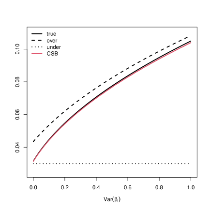
Figure 3.1. Comparison of analytical and cross-sectional bootstrap estimators of standard deviation of $\widehat{\theta}$ in this example.

We find that the standard analytical plug-in estimator overestimates the standard error for any degree of heterogeneity, whereas the analytical plug-in estimator that omits the heterogeneity in $\beta_{i}$ underestimates the standard error in the presence of any heterogeneity. The mean of cross-sectional bootstrap estimator is very close to the standard error uniformly for all the degrees of heterogeneity considered, as predicted by the asymptotic theory.

3.2.3. Simultaneous inference

The bootstrap algorithms for the model functionals presented in Appendix A are designed to construct confidence bands that cover the functionals simultaneously over the region of points of interest. For example, if we are interested in the scalar function $y\mapsto\xi(y)$ over $y\in\mathcal{Y}$, the asymptotic $p$-confidence band $\mathsf{CI}_{p}(\xi(y)):=[\widehat{\xi}_{l}(y),\widehat{\xi}_{u}(y)]$ is defined by the data dependent end-point functions $y\mapsto\widehat{\xi}_{l}(y)$ and $y\mapsto\widehat{\xi}_{u}(y)$ that satisfy

$$\Pr\left(\widehat{\xi}_{l}(y)\leq\xi(y)\leq\widehat{\xi}_{u}(y),y\in\mathcal{Y}\right)\to p\text{ as }N,T\to\infty.$$

We illustrate in Section 4 how these confidence bands can be used to test multiple hypotheses about the sign and shape of the functionals. Pointwise confidence intervals are special cases obtained by setting the region $\mathcal{Y}$ to include only one point.

4. The Dynamics of Labor Income

4.1. Data

We employ data from the Panel Study of Income Dynamics for the years 1967 to 1996 (PSID, 2020). The sample selection follows Hu et al. (2019) which restricts the sample to male heads of household working a minimum of 40 weeks. We drop the worker-year observations where labor income is above the 99 sample percentile or below the 1 sample percentile, and keep workers observed for a minimum of 15 years. This selection results in an unbalanced panel with 1,629 workers and 33,338 worker-year observations.

The variables used in the analysis include measures of labor income, years of schooling, number of children, marital status, year of birth, survey year and an indicator denoting the individual is white. The years of schooling variable is constructed from the categorical variable highest grade completed with the following equivalence: 0-5 grades = 5 years, 6-8 grades = 7 years, 9-11 grades = 10 years, 12 grades = 12 years, some college = 14 years, and college degree = 16 years. Following the literature on labor income processes, we construct the outcome, $y_{it}$, as the residuals of the pooled regression of the logarithm of annual real labor income in 1996 US dollars, deflated by the CPI-U-RS price deflator, on indicators for marital status, number of children, year of birth and survey year. We refer to these residuals as labor income.

4.2. Model coefficients

We estimate the HDR model (2.1) with $\boldsymbol{x}_{it}=(1,y_{i,t-1})^{\prime}$. We denote the model coefficients by $\boldsymbol{\beta}_{i}(y)=(\alpha_{i}(y),\rho_{i}(y))^{\prime}$ and their bias corrected estimates by $\widehat{\boldsymbol{\beta}}_{i}(y)=(\widehat{\alpha}_{i}(y),\widehat{\rho}_{i}(y))^{\prime}$, where we refer to $y\mapsto\alpha_{i}(y)$ as the intercept or level function and $y\mapsto\rho_{i}(y)$ as the slope or persistence function. These estimates are obtained using (3.1). The left panel of Figure 4.1 (Between Median) plots the kernel density of the estimated slope function $\widehat{\rho}_{i}(y)$ at a fixed value of $y$ corresponding to the sample median of $y_{it}$ pooled across workers and years. We find substantial heterogeneity between workers in this parameter. The density of the persistence coefficient includes both positive and negative values corresponding to positive and negative state dependencies in the labor income process at the median. The right panel of Figure 4.1 (Within Median) plots the pointwise sample median of the function $y\mapsto\widehat{\rho}_{i}(y)$ over a region $\mathcal{Y}$ that includes all the sample percentiles of the sample values of $y_{it}$ pooled across workers and years. The function is plotted with respect to the probability level of the sample percentile to facilitate interpretation. We find substantial heterogeneity in the slope within the distribution of the median worker. The slope is increasing with the percentile level indicating higher persistence parameter at the upper tail of the distribution. The two figures combined illustrate the existence of substantial heterogeneity in income dynamics both between and within workers.

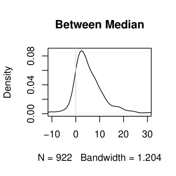
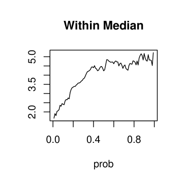
Figure 4.1. The left panel plots the cross-sectional density of $\widehat{\rho}_{i}(y)$ when $y$ is fixed to the sample median of $y_{it}$ in the pooled sample; the right panel plots the cross-sectional pointwise median of the function $y\mapsto\widehat{\rho}_{i}(y)$.

4.3. Goodness of fit

Figure 4.2 compares the empirical distributions of $y_{it}$ in 1981 and 1991 with the corresponding distributions predicted by the HDR model. The model provides a remarkably close fit to the empirical distribution for all the values of $y$, including the tails.

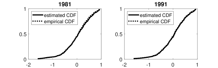
Figure 4.2. Empirical and predicted actual distributions, $F_{t}$, $t\in\{1981,1991\}$.

4.4. Projections of coefficients

We obtain projections of the estimated coefficients to explore if specific worker characteristics are associated with the heterogeneity in the level and persistence of labor income between workers. We apply (3.2) with $\boldsymbol{z}_{i}$ including a constant, the initial labor income, years of schooling, a white indicator and year of birth, and $\boldsymbol{w}_{i}=\boldsymbol{z}_{i}$.

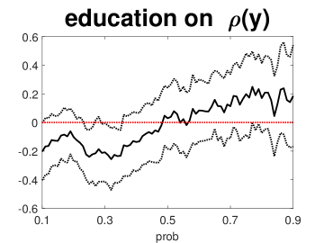
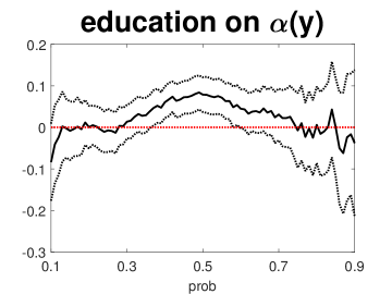
Figure 4.3. Projection coefficients of $\boldsymbol{\beta}_{i}(y)=(\rho_{i}(y),\alpha_{i}(y))$ on worker education levels. The confidence bands are obtained by cross-sectional bootstrap using Algorithm A.1 with $B=500$.

Figure 4.3 reports the estimates and 90% confidence bands of the projection coefficient function $y\mapsto\boldsymbol{\theta}(y)$ for education over a region $\mathcal{Y}$ that includes all the sample percentiles of the pooled sample of $y_{it}$ with probability levels $\{0.10,0.11,\ldots,0.90\}$, plotted with respect to these probability levels. We find the education level is associated with coefficient heterogeneity at some locations of the distribution. For example, the persistence parameter $\rho_{i}(y)$ is negatively associated with education at the bottom of the distribution, whereas the level parameter $\alpha_{i}(y)$ is positively associated with education in the middle of the distribution. The effect of education on $\rho_{i}(y)$ is increasing with $y$, although this pattern should be interpreted carefully as the function is not very precisely estimated, as reflected by the width of the confidence band.

4.5. Impact of an income shock

An important implication of the HDR representation of labor income is that an individual’s location in the income distribution in a specific time period partially depends on his location in previous periods. Moreover, the nature of this dependence varies by worker. This indicates that a shock to current labor income will determine the path of future income. To illustrate the presence and heterogeneity of this dependence we examine the impact on future income resulting from a negative shock to initial income.

We implement the shock by reducing by 25 percent the labor income in 1985. We interpret this as an unanticipated shock in that we change the level of initial income but keep all other aspects of the model constant. Specifically, we estimate the counterfactual distribution (2.4) for the transformation

$$h_{it}(\boldsymbol{x}_{it})=(1,y_{i(t-1)}+\log(1-\kappa))^{\prime}$$

with $\kappa=0.25$. This transformation yields a counterfactual distribution of labor income in $t=1986$. We also estimate the actual distribution and the corresponding quantile effects. We compare the estimates from the following alternative models:

(a) the homogeneous location-shift model: $y_{it}=\beta y_{i(t-1)}+\alpha+e_{i,t},$

(b) the homogeneous location-shift model with fixed effects: $y_{it}=\beta y_{i(t-1)}+\alpha_{i}+e_{it};$

(c) the homogeneous DR model: $P(y_{it}\leq y\mid y_{i(t-1)})=\Lambda(\beta(y)y_{i(t-1)}+\alpha(y)).$

The parameters of the location-shifts models are estimated by least squares; the parameters of the homogeneous DR model are estimated by distribution regression with $\Lambda$ equal to the standard logistic distribution.

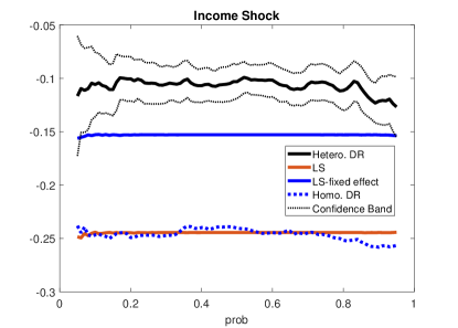
Figure 4.4. Quantile effects of counterfactual distribution of unanticipated income shock. Hetero.DR refers to the proposed approach; LS refers to the homogeneous location-shift model; LS-fixed effect additionally adds fixed effects; Homo.DR refers to the homogeneous DR model. The confidence band for the estimation of the heterogeneous DR model (the proposed approach) is also plotted.

Figure 4.4 reports estimates and 90% confidence bands of the quantile effects together with the estimates obtained from the alternative models. The confidence bands are computed using Algorithm A.3 with $p=.90$, $B=500$ and $\mathcal{T}=\{.05,.06,\ldots,.95\}$. The estimates show that the fully homogeneous location-shift and DR models predict that the income shock reduces next period income almost in a one-for-one basis throughout the distribution. The model with fixed effects lowers the effect to about 15%, whereas the HDR model further ameliorates it to about 10%. The confidence band shows that there is no evidence of heterogeneous effects across the distribution. The confidence band of the HDR model does not fully cover the estimates of the other three models. In results not reported, we find that joint confidence bands from these models do not fully overlap with the confidence bands of the HDR model. We can formally reject the homogeneity restrictions imposed by the alternative models.

4.6. Dynamic aspects of relative poverty

We now analyze labor income mobility and the existence of “relative poverty” traps. We evaluate the probability of remaining in lower locations of the residual distribution noting that we refer to this as relative poverty as we acknowledge that the total income level may not be below the poverty line. We do so via the model from Section 2.4.1, where the conditional distribution is represented by a discrete Markov chain. We set the states for each worker as the observed values of $y_{it}$, that is $\mathcal{Y}_{i}:=\{y_{it}:t=1,...,T\}$ and $K=T$.

Following Hu et al. (2019), consider the following probabilities to describe mobility

$$P_{i}(p,q,h):=\Pr(y_{i(t+h)}<y_{p}\mid y_{it}<y_{q},\mathcal{F}_{it}),\quad i=1,...,N,$$

where $y_{p}$ and $y_{q}$ are the $p$-quantile and $q$-quantile of the distribution of labor income. These probabilities correspond to the following experiment: If we exogenously set labor income below $y_{q}$ at time $t$, then $P_{i}(p,q,h)$ is the probability labor income is below $y_{p}$ after $h$ years. For example, if we define the poverty line as the $10$-percentile, then $P_{i}(0.1,0.1,5)$ is the probability that worker $i$ would remain in poverty after 5 years if he falls below the poverty line due to, for example, a negative income shock.

Our model allows the probabilities $P_{i}(p,q,h)$ to be heterogeneous across workers. To summarize this heterogeneity, we can examine the average probability

$$\bar{P}(p,q,h) = \frac{1}{N}\sum_{i=1}^{N}P_{i}(p,q,h).$$

For instance, $\bar{P}(0.3,0.1,1)$ is the probability that a randomly chosen worker is below the 30-percentile if in the previous year he was below the 10-percentile. We also examine quantiles of the probabilities such as

$$Q_{\tau}(p,q,h)$$

which denotes the $\tau$-quantile of $\{P_{i}(p,q,h):,i=1,...,N\}$ for fixed $(p,q,h)$. For example, $Q_{0.25}(0.3,0.1,1)$ is the first quartile of the probability that a worker is below the 30-percentile if in the previous year he was below the 10-percentile.

The upper panel of Figure 4.6 plots $p\mapsto\bar{P}(p,q,h)$ for $p\in[0,0.5]$, $q\in\{0.1,0.25,0.5\}$ and $h\in\{1,2,5\}$. We find heterogeneity with respect to the initial condition that vanishes with time due to the ergodicity of the process. The probability that a randomly selected worker remains below the 10-percentile after one year is more than 50%, whereas this probability decreases by about half if the worker was initially below the median. This difference in probabilities reduces after two years and almost vanishes after five years. The lower panel of Figure 4.6 plots $p\mapsto Q_{\tau}(p,q,h)$ for $p\in[0,0.5]$, $q=0.1$, $h\in\{1,2,5\}$ and $\tau\in\{0.1,0.5,0.9\}$. We uncover significant heterogeneity across workers that is hidden in the analysis of the mean worker. Even after 5 periods the deciles of the probability of remaining below the 10-percentile range from $0$ to more than $0.9$. This illustrates the importance of accounting for heterogeneity in understanding labor income risk.

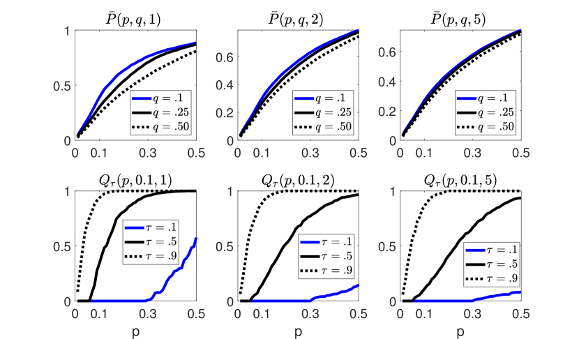
Figure 4.5. Means and quantiles of probabilities of income mobility. The upper panels report $\bar{P}(p,q,h)$ and the lower panels report $Q_{\tau}(p,q,h).$

Let $h_{i}(p)$ denote the recurrence time of $y_{p}$, that is, starting from $\{y_{it}<y_{p}\}$, the number of years $h$ until the first occurrence of $\{y_{i(t+h)}>y_{p}\}$. For example, if $y_{0.10}$ is the poverty line, $h_{i}(0.10)$ is a random variable that measures the number of years that worker $i$ takes to escape from poverty. Then,

$$\Pr(h_{i}(p)=h)=\Pr(y_{i(t+h)}>y_{p},y_{i(t+h-1)}<y_{p},...,y_{i(t+1)}<y_{p}\mid y_{it}<y_{p},\mathcal{F}_{it}),$$

which can be expressed as a functional of the parameters of the HDR model. Another interesting quantity is

$$H_{i}(p)=\sum_{h}h\Pr(h_{i}(p)=h),$$

which gives the expected recurrence time for each individual. In the previous example, $H_{i}(0.10)$ gives the expected number of years that worker $i$ would take to escape from poverty. Figure 4.6 plots a histogram of the estimated $H_{i}(0.10)$. More than 60% of the workers would escape from the poverty in two or less years, but about 10% of the workers would stay for more than 20 years. Table 4.1 reports several quantiles of the estimated $H_{i}(0.1)$ for groups stratified by education and race. We find substantial heterogeneity between workers associated with education and race. Whereas the deciles of the expected recurrence time range from 1 to 7 years for workers with at least high school, the corresponding value of 176 years indicates there are more than 10% of workers with less than high school that would never escape poverty. The distribution of the expected recurrence time also differs by race. The upper decile of the expected recurrence time is about 20 years higher for nonwhite than for white workers. This heterogeneity in the persistence of poverty has clear implications for the design of poverty alleviation policies. As they employ a different sample to ours and employ a different definition of “relative poverty” we do not directly compare these results to Lillard and Willis (1978). However, in addition to confirming the dependence in labor income documented in their study, we illustrate the remarkable difficulty facing some workers in escaping relative poverty.

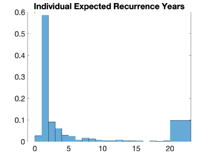
Figure 4.6. Histogram of expected recurrence time out-of-poverty in years, $H_{i}(0.10)$

Table 4.1. Quantiles of expected recurrence time out-of-poverty in years, $H_{i}(0.10)$, by education and racial groups

	Quantiles
	0.10	0.25	0.50	0.75	0.90
All	1.00	1.00	1.47	3.63	19.45
Edu$<12$ years	1.00	1.35	2.92	9.75	175.8
Edu$\geq 12$ years	1.00	1.00	1.20	2.39	7.37
White	1.00	1.00	1.27	3.12	13.88
non-White	1.00	1.11	1.81	5.52	33.91

4.7. Impact of completing high school

We now evaluate a hypothetical scenario in which workers with less than 12 years of schooling are assigned a high school degree (12 years of schooling). This also reflects a form of partial equilibrium analysis as the model parameters and the income distribution are based on the pre-intervention setting and we do not allow for possible general equilibrium effects. We assume that the resulting distribution is (2.4) with $h(\boldsymbol{x}_{it})=\boldsymbol{x}_{it}$ and $g$ defined in (2.5). We set the values of $y_{i(t-1)}$ to the observed values in 1985 and assume that the change occurs at the beginning of 1986. We estimate the actual and counterfactual distributions in 1986 using (3.3), and the short and long term quantile effects using (3.6). To estimate the stationary distributions, we set the states for each worker in the Markov chain to the observed values of $y_{it}$, that is $\mathcal{Y}_{i}:=\{y_{it}:t=1,...,T\}$ and $K=T$.

Figure 4.7 reports estimates and 90% confidence bands of $\mathsf{QE}_{t}$ in the left panel and $\mathsf{QE}_{\infty}$ in the right panel. The confidence bands are computed using Algorithm A.3 with $p=.90$, $B=500$ and $\mathcal{T}=\{.05,.06,\ldots,.95\}$. We find this intervention has heterogeneous effects across the distribution. The lower tail increases by around 7.5% after one year to almost 15% in the long run, whereas there is very little effect at the upper tail both in the short and long run. The confidence bands show that the results at the lower tail are statistically significant and allow us to formally reject the hypothesis of constant effects across the distribution. The magnitudes of the effects are economically noteworthy given the policy affects a relatively small fraction of the population. The results indicate that the increase in education for those with lower levels of education shifts the bottom tail of the labor income distribution of the entire population. This supports the commonly held policy view that increasing education of the lowly educated will reduce the level of inequality. There is no evidence of movements in the distribution at higher levels of labor income.

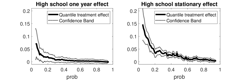
Figure 4.7. Quantile effects of counterfactual high school policy.

5. Asymptotic Theory

This section develops asymptotic theory for the estimators of the functionals of interest. We start by introducing some notation. Recall that the loss function for the estimation of the coefficients is: $Q_{y,i}(b)=T^{-1}\sum_{t=1}^{T}q_{y,it}(b)$, where

$$q_{y,it}(b)=1\{y_{it}\leq y\}\Lambda(-\boldsymbol{x}_{it}^{\prime}b)+1\{y_{it}>y\}[1-\Lambda(-\boldsymbol{x}_{it}^{\prime}b)].$$

Let

$$\psi_{it}(y) = \nabla q_{y,it}(\boldsymbol{\beta}_{i}(y))$$

$$\varpi_{it}^{d}(y) = \nabla^{d}q_{y,it}(\boldsymbol{\beta}_{i}(y))-\mathbb{E}\nabla^{d}q_{y,it}(\boldsymbol{\beta}_{i}(y)),\quad d=1,2,3.$$

$$\mathbb{A}_{1i}(y) = [\mathbb{E}\nabla^{2}q_{y,it}(\boldsymbol{\beta}_{i}(y))]^{-1},\quad\mathbb{A}_{2i}(y)=\mathbb{E}\nabla^{3}q_{y,it}(\boldsymbol{\beta}_{i}(y)),$$

where all terms are defined using the true $\boldsymbol{\beta}_{i}(y)$. Specifically, when $\beta$ is a vector, the third order derivative matrix $\nabla^{3}q(\beta)$ is a $d_{\beta}\times d_{\beta}^{2}$ matrix, defined as $(\nabla B_{1}(\beta),...,\nabla B_{d_{\beta}}(\beta))$, where $B_{j}(\beta)$ is the $d_{\beta}\times d_{\beta}$ Jacobian of the $j$ th row of $\nabla^{2}q$, here $d_{\beta}:=\dim(\beta)$.

5.1. Sampling

The following assumptions relate to the properties of the sampling process. Recall that $\mathcal{F}_{i1}\subset...\subset\mathcal{F}_{iT}$ is the sequence of filtrations over time that include covariates and any time invariant variables for unit $i$.

Assumption 5.1 (Cross-section dimension).

(i) $\mathbb{E}(\gamma_{i}(y_{1})|\boldsymbol{w}_{i},\psi_{it}(y_{2}))=0$ for any $y_{1},y_{2}$ and $i=1,...,N.$

(ii) The filtrations $\mathcal{F}_{iT}$ are independent across $i=1,...,N$.

(iii) $\{(Y_{it},\boldsymbol{x}_{it},\boldsymbol{w}_{t}):t\leq T\}$ are identically distributed across $i=1,...,N$.

Assumption 5.2 (Time series dimension).

There are universal constants $C,c>0$ such that almost surely,

$$\max_{i\leq N}\mathbb{E}\left[\sup_{y\in\mathcal{Y}}\|\frac{1}{\sqrt{T}}\sum_{t}\varpi^{d}_{it}(y)\|^{8+c}\right]<C,$$

$$\max_{i\leq N}\mathbb{E}\left[\sup_{|y_{1}-y_{2}|\leq\epsilon}\|\frac{1}{\sqrt{T}}\sum_{t}\varpi^{d}_{it}(y_{1})-\frac{1}{\sqrt{T}}\sum_{t}\varpi^{d}_{it}(y_{2})\|^{8}\right]<C\epsilon^{2},$$

for $d=1,2,3.$

Assumption 5.2 imposes conditions regarding serial dependence. We impose two high level conditions regarding the empirical process for weakly dependent data. It requires some primitive conditions, e.g., mixing conditions, so that $\{(Y_{it},\boldsymbol{x}_{it}):t\leq T\}$ is serially weakly dependent.

5.2. Projections of coefficients

The main result of this section is to show $\widehat{\boldsymbol{\theta}}(y)-\boldsymbol{\theta}(y)$ converges to a Gaussian process.

We start by defining the covariance kernel of the limiting process of $\widehat{\theta}-\theta$. For a given integer $M>0$, let $Y_{M}=(y_{1},...,y_{M})^{\prime}$ be an arbitrary $M$-dimensional vector on $\otimes_{i=1}^{M}\mathcal{Y}.$ Let $S_{wz}:=C_{1}^{-1}C_{2}(C_{2}^{\prime}C_{1}^{-1}C_{2})^{-1}$ where $C_{1}=\mathbb{E}\boldsymbol{w}_{i}\boldsymbol{w}_{i}^{\prime}$, $C_{2}=\mathbb{E}\boldsymbol{w}_{i}\boldsymbol{z}_{i}^{\prime}$, and

$$V_{\psi}(y_{k},y_{l}) = \mathbb{E}\left\{(S_{wz}^{\prime}\boldsymbol{w}_{i}\boldsymbol{w}_{i}^{\prime}S_{wz})\otimes\left[\mathbb{A}_{1i}(y_{k})\mathbb{E}(\frac{1}{T}\sum_{s,t\leq T}\psi_{it}(y_{k})\psi_{it}(y_{l})^{\prime}|\boldsymbol{w}_{i})\mathbb{A}_{1i}(y_{l})\right]\right\}$$ (5.1)

$$V_{\gamma}(y_{k},y_{l}) = \mathbb{E}\left\{(S_{wz}^{\prime}\boldsymbol{w}_{i}\boldsymbol{w}_{i}^{\prime}S_{wz})\otimes\mathbb{E}(\gamma_{i}(y_{k})\gamma_{i}(y_{l})^{\prime}\mid\boldsymbol{w}_{i})\right\}$$ (5.2)

$$\Sigma_{NT}(y_{k},y_{l}) = \frac{1}{NT}V_{\psi}(y_{k},y_{l})+\frac{1}{N}V_{\gamma}(y_{k},y_{l})$$ (5.3)

$$\Sigma_{NT}(y) = \Sigma_{NT}(y,y).$$ (5.4)

The covariance kernel is now given by the limit of the elements of the following $M\times M$ matrix

$$H_{\eta,NT}=(H_{\eta,NT}(y_{k},y_{l}))_{M\times M}$$

where

$$H_{\eta,NT}(y_{k},y_{l})=\frac{\eta^{\prime}\Sigma_{NT}(y_{k},y_{l})\eta}{[\eta^{\prime}\Sigma_{NT}(y_{k})\eta]^{1/2}[\eta^{\prime}\Sigma_{NT}(y_{l})\eta]^{1/2}}$$

and $\eta\in\mathbb{R}^{\dim(\mathsf{vec}\theta)}$. We make the following assumptions about the covariance kernel:

Assumption 5.3 (Covariance kernel).

For any $\eta\in\mathbb{R}^{\dim(\mathsf{vec}\theta)}$ and $\|\eta\|>c>0$, any integer $M>0$, and any $M$-dimensional vector $Y_{M}=(y_{1},...,y_{M})^{\prime}$ on $\otimes_{i=1}^{M}\mathcal{Y}$, there is an $M\times M$ matrix $H_{\eta}$, such that almost surely,

$$\lim_{N,T\to\infty}H_{\eta,NT}=H_{\eta}.$$ (5.5)

In addition, there is $c_{Y_{M},\eta}>0$ such that

$$\lambda_{\min}(H_{\eta})>c_{Y_{M},\eta}.$$ (5.6)

Here $c_{Y_{M},\eta}$ may depend on $Y_{M},M$ and $\eta.$

Condition (5.6) is used to establish the finite dimensional distribution (f.i.d.i.) of $\eta^{\prime}\mathsf{vec}(\widehat{\theta}(\cdot)-\theta(\cdot))$, which is required for a given $Y_{M},M$ and $\eta$. Therefore, the constant $c_{Y_{M},\eta}$ is allowed to depend on these parameters. To show that Assumption 5.3 is reasonable even though the variance of $\gamma_{i}(y)=\boldsymbol{\beta}_{i}(y)-\boldsymbol{\theta}(y)\boldsymbol{z}_{i}$ may vary across $y$ in the second-stage regression, we consider the following model

$$\gamma_{i}(y) = \xi_{NT}(y)\bar{\gamma}_{i}(y),\quad\forall y\in\mathcal{Y},\forall i\leq N$$ (5.7)

$$V_{\gamma}(y_{k},y_{l}) = \xi_{NT}(y_{k})\xi_{NT}(y_{l})V_{\bar{\gamma}}(y_{k},y_{l}),\quad\inf_{y}\lambda_{\min}(V_{\bar{\gamma}}(y,y))>c.$$ (5.8)

Here $\xi_{NT}(y)$ is a bounded non-stochastic sequence that may converge to zero, whose rate depends on $y$; $\bar{\gamma}_{i}(y)$ is a random vector of “normalized” $\gamma_{i}(y)$ , so $V_{\bar{\gamma}}(y,y)$ can be understood as a normalized covariance matrix. Hence the strength of $\gamma_{i}(y)$ is determined by the rate of convergence of $\xi_{NT}(y)$. Given this setting, consider the following special cases:

Case 1:

$\xi_{NT}(y_{k})=o(T^{-1/2})$ and $\xi_{NT}(y_{l})\gg T^{-1/2}$. Here the explanatory power of $\boldsymbol{w}_{i}$ is strong for $\beta_{i}(y_{k})$, but relatively weak for $\beta_{i}(y_{l})$. Then

$$\lim_{N,T\to\infty}H_{\eta,NT}(y_{k},y_{l})=0.$$

Note that the opposite case of $\xi_{NT}(y_{k})\gg o(T^{-1/2})$ and $\xi_{NT}(y_{l})=T^{-1/2}$ is also covered.

Case 2:

Both $\xi_{NT}(y_{k}),\xi_{NT}(y_{l})\gg T^{-1/2}$. Here the explanatory power of $\boldsymbol{w}_{i}$ is strong for both $\beta_{i}(y_{k})$ and $\beta_{i}(y_{l})$. Then

$$\lim_{N,T\to\infty}H_{\eta,NT}(y_{k},y_{l})=\lim_{N\to\infty}\frac{\eta^{\prime}V_{\bar{\gamma}}(y_{k},y_{l})\eta}{[\eta^{\prime}V_{\bar{\gamma}}(y_{k},y_{k})\eta]^{1/2}[\eta^{\prime}V_{\bar{\gamma}}(y_{l},y_{l})\eta]^{1/2}},$$

where the limit of the right hand side is assumed to exist.

Case 3:

Both $\xi_{NT}(y_{k}),\xi_{NT}(y_{l})\ll T^{-1/2}$. Here the explanatory power of $\boldsymbol{w}_{i}$ is relatively weak for both $\beta_{i}(y_{k})$ and $\beta_{i}(y_{l})$. Then

$$\lim_{N,T\to\infty}H_{\eta,NT}(y_{k},y_{l})=\lim_{N\to\infty}\frac{\eta^{\prime}V_{\psi}(y_{k},y_{l})\eta}{[\eta^{\prime}V_{\psi}(y_{k},y_{k})\eta]^{1/2}[\eta^{\prime}V_{\psi}(y_{l},y_{l})\eta]^{1/2}},$$

where the limit of the right hand side is assumed to exist.

So each element has a limit given on the right hand side. With sufficient variations (across $y_{k}$), one may assume the limit of the matrix $H_{\eta,NT}$ is non-degenerate that satisfies (5.6).

The following condition describes the continuity of some moment functions. For notational simplicity, we write

$$V_{\gamma}(y):=V_{\gamma}(y,y),\quad V_{\psi}(y):=V_{\psi}(y,y).$$

Assumption 5.4 (Continuity).

There is a universal constant $C>0$ such that for all $y_{1},y_{2}\in\mathcal{Y}$,

$$\|V_{\psi}(y_{1})-V_{\psi}(y_{2})\|+\max_{i\leq N}\|\mathbb{A}_{d,i}(y_{1})-\mathbb{A}_{d,i}(y_{2})\|<C|y_{1}-y_{2}|,\quad d=1,2.$$

In addition, for all $\epsilon>0,$

$$\frac{1}{N}\sum_{i=1}^{N}\mathbb{E}\left[\sup_{|y_{1}-y_{2}|<\epsilon}\frac{\|\gamma_{i}(y_{1})\boldsymbol{w}_{i}^{\prime}-\gamma_{i}(y_{2})\boldsymbol{w}_{i}^{\prime}\|^{4}}{M(y_{1},y_{2})^{2}}\right]<C\epsilon$$

$$\sup_{|y_{1}-y_{2}|<\epsilon}\frac{\|V_{\gamma}(y_{1})-V_{\gamma}(y_{2})\|}{M(y_{1},y_{2})}\leq C\epsilon.$$

where $M(y_{1},y_{2}):=\min\{\lambda_{\min}(V_{\gamma}(y_{1})),\lambda_{\min}(V_{\gamma}(y_{2}))\}$.

Assumption 5.5 (Moment bounds).

There are universal constants $C,c>0$ so that

(i) For some $a>0$,

$$\mathbb{E}\left[\sup_{y\in\mathcal{Y}}\left(\frac{\|\gamma_{i}(y)\boldsymbol{w}_{i}^{\prime}\|}{\lambda^{1/2}_{\min}(V_{\gamma}(y))}\right)^{4}\right]<C.$$

(ii) Let $\Theta$ be the parameter space for $\{\beta_{1}(y),...,\beta_{N}(y):y\in\mathbb{R}\}$. The following moment bounds hold:

(a) $\max_{i\leq N}\sup_{y\in\mathcal{Y}}[\|\mathbb{A}_{1i}(y)\|+\|\mathbb{A}_{2i}(y)\|]<C$

(b) $\sup_{y}\sup_{b\in\Theta}\max_{i\leq N}[\|\nabla^{3}Q_{y,i}(b)\|+\|\nabla^{4}Q_{y,i}(b)\|+\|(\nabla^{2}Q_{y,i}(b))^{-1}\|]=O_{P}(1)$

(c) $\max_{i\leq N}\mathbb{E}\|\boldsymbol{w}_{i}\|^{8+c}<C$.

(iii) For all $y\in\mathcal{Y}$, and all $i=1,...,N$, we have $\min_{t\leq T}y_{it}<y<\max_{t\leq T}y_{it}$ with probability approaching one.

(iv) Let $S_{\psi,i}(y)=\mathsf{Var}\left(\frac{1}{\sqrt{T}}\sum_{t=1}^{T}\psi_{it}(y)|\boldsymbol{w}_{i}\right)$. Then almost surely,

$$\min_{i}\inf_{y\in\mathcal{Y}}\lambda_{\min}(S_{\psi,i}(y))>c.$$

In addition, all eigenvalues of $C_{1}$ and $C_{2}^{\prime}C_{2}$ are bounded away from zero and infinity, where $C_{1}=\mathbb{E}\boldsymbol{w}_{i}\boldsymbol{w}_{i}^{\prime}$ and $C_{2}=\mathbb{E}\boldsymbol{w}_{i}\boldsymbol{z}_{i}^{\prime}$, with $\mathsf{rank}(C_{2})\geq\dim(\boldsymbol{z}_{i})$.

(v) $\frac{1}{T}\sum_{t}\mathbb{E}_{i}\boldsymbol{x}_{it}\boldsymbol{x}_{it}^{\prime}$ is of full rank for each $i$, where the expectation $\mathbb{E}_{i}$ is taken with respect to the joint density of $(\boldsymbol{x}_{i1},...,\boldsymbol{x}_{iT})$ conditional on $\mathcal{F}_{i1}$.

Condition (i) of this assumption requires that the fourth moment of $\gamma_{i}(y)$ is bounded by its second moment up to a constant, uniformly in $y$. To see the plausibility of this condition, again consider model (5.7). Then the left hand side of condition (i) becomes

$$\mathbb{E}\left[\sup_{y\in\mathcal{Y}}\left(\frac{\|\gamma_{i}(y)\boldsymbol{w}_{i}^{\prime}\|^{2}}{\lambda_{\min}(V_{\gamma}(y))}\right)^{2}\right]=\frac{\frac{1}{N}\sum_{i=1}^{N}\mathbb{E}(\|\bar{\gamma}_{i}(y)\boldsymbol{w}_{i}^{\prime}\|^{4})}{\inf_{y\in\mathcal{Y}}\lambda_{\min}^{2}(V_{\bar{\gamma}}(y,y))},$$

which is upper bounded by a constant provided $\frac{1}{N}\sum_{i=1}^{N}\mathbb{E}(\|\bar{\gamma}_{i}(y)\boldsymbol{w}_{i}^{\prime}\|^{4})<C.$ Other conditions of this assumption are standard. Condition (iii) requires that we only focus on $y\in\mathcal{Y}$ that are in the range of the observed outcomes. Finally, conditions (iv) and (v) of Assumption 5.5 identify the parameters $\theta(y)$ and $\boldsymbol{\beta}_{i}(y)$. To see this, note that the model implies

$$-\frac{1}{T}\sum_{t=1}^{T}\mathbb{E}_{i}\boldsymbol{x}_{it}\Lambda^{-1}\left(\Pr(y_{it}\leq y|\mathcal{F}_{it})\right)=\left(\frac{1}{T}\sum_{t=1}^{T}\mathbb{E}_{i}\boldsymbol{x}_{it}\boldsymbol{x}_{it}^{\prime}\right)\boldsymbol{\beta}_{i}(y).$$

Inverting $\frac{1}{T}\sum_{t=1}^{T}\mathbb{E}_{i}\boldsymbol{x}_{it}\boldsymbol{x}_{it}^{\prime}$ leads to the identification of $\boldsymbol{\beta}_{i}(y)$. In addition, $\mathsf{rank}(C_{2})\geq\dim(\boldsymbol{z}_{i})$ implies the identification of $\boldsymbol{\theta}(y).$

In the theorem below, $L$ denotes the number of lags used for the Newey-West truncation for long-run variance, which is needed for analytical bias corrections.

Theorem 5.1.

Suppose $N=o(T^{2})$ and $NL^{2}=o(T^{3})$. Assumptions 5.1-5.5 hold. If $\boldsymbol{\beta}_{i}(y)$ is estimated using Jackknife-debias, then we additionally assume Assumption LABEL:assa.1. For any $\eta$ such that $\|\eta\|>c>0$,

$$\frac{\eta^{\prime}\mathsf{vec}(\widehat{\theta}(\cdot)-\theta(\cdot))}{\left[\eta^{\prime}\Sigma_{NT}(\cdot)\eta\right]^{1/2}}\Rightarrow\mathbb{G}(\cdot)$$

where $\Sigma_{NT}(y)=\frac{1}{NT}V_{\psi}(y)+\frac{1}{N}V_{\gamma}(y)$ and $\mathbb{G}(\cdot)$ is a centered Gaussian process with a covariance function $H(y_{k},y_{l})$ as the $(k,l)$ element of $H_{\eta}$.

5.3. Counterfactual distributions and quantile effects

For a generic estimator $\widehat{F}(y)$ of $F(y)$, which may be one of the cross-sectional distributions that we discussed earlier, one can show that it has the following expansion

$$\widehat{F}(y)-F(y)=\frac{1}{N}\sum_{i=1}^{N}[\frac{1}{\sqrt{T}}d_{\psi,i}(y)+d_{\gamma,i}(y)]+o_{P}(\zeta_{NT}(y))$$

where $\zeta_{NT}(y)=(NT)^{-1/2}+N^{-1/2}\mathsf{Var}_{t}(d_{\gamma,i})^{1/2}$, and the two leading terms $d_{\psi,i}(y)$ and $d_{\gamma,i}(y)$ are asymptotically independent, and respectively capture the sampling variation from the first-stage and second-stage. The quantile effects have similar expansions

$$\widehat{\mathsf{QE}}(\tau)-\mathsf{QE}(\tau) = \frac{1}{N}\sum_{i=1}^{N}[\frac{1}{\sqrt{T}}p_{\psi,i}(\tau)+p_{\gamma,i}(\tau)]+o_{P}(\bar{\zeta}_{NT}(\tau))$$ (5.9)

where $\bar{\zeta}_{NT}(\tau)=(NT)^{-1/2}+N^{-1/2}\mathsf{Var}_{t}(p_{\gamma,i}(\tau))^{1/2}$, and $p_{\psi,i}(\tau)$ and $p_{\gamma,i}(\tau)$ are zero-mean uncorrelated terms.

We make the following additional assumptions, which are assumed to hold for all $\widetilde{\boldsymbol{x}}_{it}\in\{\boldsymbol{x}_{it},h_{it}(\boldsymbol{x}_{it})\}$, i.e., either the original variable $\boldsymbol{x}_{it}$ or the counterfactual $h_{it}(\boldsymbol{x}_{it})$. The formal definitions of $(d_{\psi,i},d_{\gamma,i},p_{\psi,i},p_{\gamma,i})$ depend on the specific $F\in\{F_{t},G_{t},F_{\infty},G_{\infty}\}$ and $\mathsf{QE}\in\{\mathsf{QE}_{t},\mathsf{QE}_{\infty}\}$, which are given in the Appendix. We emphasize that $F_{t},G_{t}$ respectively denote the actual and counterfactual distributions at time $t$ and $F_{\infty},G_{\infty}$ respectively denote the actual and counterfactual stationary distributions.

Let $\dot{\Lambda}(s)=\frac{d}{ds}\Lambda(s)$ and $\ddot{\Lambda}(s)=\frac{d^{2}}{ds^{2}}\Lambda(s)$.

Assumption 5.6 (Moment bounds).

(i) $\sup_{s}|\dot{\Lambda}(s)|+\sup_{s}|\ddot{\Lambda}(s)|<C$.

(ii) $\mathbb{E}[\psi_{it}(y_{k})|\beta_{i}(y_{l}),\widetilde{\boldsymbol{x}}_{it},\boldsymbol{z}_{i},\boldsymbol{w}_{i},\gamma_{i}(y_{l})]=0$ for any $y_{k},y_{l}\in\mathcal{Y}.$

(iii) $\mathbb{E}_{t}\|\widetilde{\boldsymbol{x}}_{it}\|^{8}+\mathbb{E}\|\boldsymbol{x}_{it}\|^{8}\|g(\boldsymbol{z}_{i})-\boldsymbol{z}_{i}\|^{8}<C.$

(iv)

$$\mathbb{E}_{t}\sup_{y}\left[\frac{d_{\gamma,i}(y)}{\mathsf{Var}_{t}(d_{\gamma,i}(y))^{1/2}}\right]^{4}<C,\quad\inf_{y}\lambda_{\min}(\mathsf{Var}_{t}(d_{\psi,i}(y)))>c>0.$$

Assumption 5.7 (Continuity).

(i) There are $C>0$ and $k\geq 4$, for any $y_{1},y_{2}\in\mathcal{Y}$,

$$\mathbb{E}_{t}|\ddot{\Lambda}(-\widetilde{\boldsymbol{x}}_{it}^{\prime}\beta_{i}(y_{1}))-\ddot{\Lambda}(-\widetilde{\boldsymbol{x}}_{it}^{\prime}\beta_{i}(y_{2}))|^{k}\|\widetilde{\boldsymbol{x}}_{it}\|^{2k}\leq C|y_{1}-y_{2}|^{k}$$

$$\mathbb{E}_{t}|\dot{\Lambda}(-\widetilde{\boldsymbol{x}}_{it}^{\prime}\beta_{i}(y_{1}))-\dot{\Lambda}(-\widetilde{\boldsymbol{x}}_{it}^{\prime}\beta_{i}(y_{2}))|^{k}\|\widetilde{\boldsymbol{x}}_{it}\|^{k}\leq C|y_{1}-y_{2}|^{k}$$

$$\mathbb{E}_{t}|\ddot{\Lambda}(-\boldsymbol{x}_{it}^{\prime}\beta^{g}_{i}(y_{1}))-\ddot{\Lambda}(-\boldsymbol{x}_{it}^{\prime}\beta^{g}_{i}(y_{2}))|^{k}\|\boldsymbol{x}_{it}\|^{2k}\leq C|y_{1}-y_{2}|^{k}$$

$$\mathbb{E}_{t}|\dot{\Lambda}(-\boldsymbol{x}_{it}^{\prime}\beta^{g}_{i}(y_{1}))-\dot{\Lambda}(-\boldsymbol{x}_{it}^{\prime}\beta^{g}_{i}(y_{2}))|^{k}\|\boldsymbol{x}_{it}\|^{k}\leq C|y_{1}-y_{2}|^{k}$$

$$\mathbb{E}_{t}|\dot{\Lambda}(-\boldsymbol{x}_{it}^{\prime}\beta^{g}_{i}(y_{1}))-\dot{\Lambda}(-\boldsymbol{x}_{it}^{\prime}\beta^{g}_{i}(y_{2}))|\|\boldsymbol{x}_{it}[g(\boldsymbol{z}_{i})-\boldsymbol{z}_{i}]^{\prime}\|\leq C|y_{1}-y_{2}|.$$

(ii) There is $C>0$, for all $\epsilon>0$,

$$\sup_{|y_{1}-y_{2}|<\epsilon}\frac{|\mathsf{Var}_{t}(d_{\gamma,i}(y_{1}))-\mathsf{Var}_{t}(d_{\gamma,i}(y_{2}))|}{M(y_{1},y_{2})}\leq C\epsilon$$

$$\sup_{|\tau_{1}-\tau_{2}|<\epsilon}\frac{|\mathsf{Var}_{t}(p_{\gamma,i}(\tau_{1}))-\mathsf{Var}_{t}(p_{\gamma,i}(\tau_{2}))|}{M_{2}(\tau_{1},\tau_{2})}\leq C\epsilon$$

$$\mathbb{E}_{t}\left[\sup_{|y_{1}-y_{2}|<\epsilon}\frac{|d_{\gamma,i}(y_{1})-d_{\gamma,i}(y_{2})|^{4}}{M(y_{1},y_{2})^{2}}\right]<C\epsilon.$$

where $M(y_{1},y_{2})=\mathsf{Var}_{t}(d_{\gamma,i}(y_{1}))^{1/2}\mathsf{Var}_{t}(d_{\gamma,i}(y_{2}))^{1/2}$ and $M_{2}(\tau_{1},\tau_{2})=\mathsf{Var}_{t}(p_{\gamma,i}(\tau_{1}))^{1/2}$ $\mathsf{Var}_{t}(p_{\gamma,i}(\tau_{2}))^{1/2}$.

We present the notation of $(d_{\gamma,i},d_{\psi,i},p_{\gamma,i},p_{\psi,i})$ for all objects of interest in the appendix. The theorems below additionally require Assumptions LABEL:ase.48, LABEL:ass:g.1, which are based on some additional notation for the stationary distribution. We present them in the appendix.

Theorem 5.2.

Suppose the assumptions of Theorem 5.1 and Assumptions 5.6-5.7, LABEL:ass:g.1 hold. Then for $F\in\{F_{t},G_{t},F_{\infty},G_{\infty}\}$ and $\widehat{F}\in\{\widehat{F}_{t},\widehat{G}_{t},\widehat{F}_{\infty},\widehat{G}_{\infty}\}$, we have

$$\frac{\widehat{F}(\cdot)-F(\cdot)}{\upsilon_{NT}(\cdot)}\Rightarrow\mathbb{G}(\cdot)$$

where $v_{NT}^{2}(y)=\frac{1}{NT}\mathsf{Var}_{t}(d_{\psi,i}(y))+\frac{1}{N}\mathsf{Var}_{t}(d_{\gamma,i}(y))$ and $\mathbb{G}(\cdot)$ is a centered Gaussian process with covariance kernel function

$$\lim_{N,T}\frac{v^{2}_{NT}(y_{k},y_{l})}{v_{NT}(y_{k})v_{NT}(y_{l})},\quad v^{2}_{NT}(y_{k},y_{l}):=\frac{1}{NT}\mathbb{E}_{t}d_{\psi,i}(y_{k})d_{\psi,i}(y_{l})+\frac{1}{N}\mathbb{E}_{t}d_{\gamma,i}(y_{k})d_{\gamma,i}(y_{l}),$$

assuming that $\lim_{NT}$ exists for each pair $(y_{k},y_{l})$.

Theorem 5.3.

Suppose the assumptions of Theorem 5.2 and Assumption LABEL:ase.48 hold. Assume also, for $F\in\{F_{t},G_{t}\}$, $F$ is continuously differentiable, whose density (denoted by $\dot{F}$) satisfies $\inf_{\tau}\inf_{|y-\phi(F,\tau)|<C}\dot{F}(y)>c$ for some $C,c>0$.

Then

$$\frac{\widehat{\mathsf{QE}}_{t}(\cdot)-\mathsf{QE}_{t}(\cdot)}{J_{NT}(\cdot)}\Rightarrow\mathbb{G}_{\mathsf{QE}}(\cdot),$$

where $J_{NT}^{2}(y):=J_{NT}^{2}(y,y)$, with

$$J^{2}_{NT}(y_{k},y_{l}):=\frac{1}{NT}\mathbb{E}_{t}p_{\psi,i}(y_{k})p_{\psi,i}(y_{l})+\frac{1}{N}\mathbb{E}_{t}p_{\gamma,i}(y_{k})p_{\gamma,i}(y_{l}),$$

and $\mathbb{G}_{\mathsf{QE}}(\cdot)$ is a centered Gaussian process with covariance kernel function

$$\lim_{N,T}\frac{J^{2}_{NT}(y_{k},y_{l})}{J_{NT}(y_{k})J_{NT}(y_{l})},$$

assuming that $\lim_{NT}$ exists for each pair $(y_{k},y_{l})$.

5.4. Discussion of asymptotic behavior

To discuss the asymptotic behavior of the estimators, we closely examine one of the counterfactual effects and the new uniformity in our econometric inference problem. The asymptotic properties of other estimators are very similar.

Consider the case $\boldsymbol{z}_{i}$ is transformed into $g(\boldsymbol{z}_{i})$ in the counterfactual experiment, so that the heterogeneous coefficient is transformed to $\boldsymbol{\beta}_{i}^{g}(y)=\boldsymbol{\theta}(y)g(\boldsymbol{z}_{i})+\boldsymbol{\gamma}_{i}(y)$. In this case, expansion (5.9) holds, with two leading terms $\frac{1}{\sqrt{T}}p_{\psi,i}$ and $p_{\gamma,i}$. The first term arises from estimation of $\boldsymbol{\beta}_{i}(y)$. The second term is due to the cross-sectional projection, whose asymptotic behavior depends on three terms:

$$p_{\gamma,i}(\tau) \text{depends on }(a),(b),(c),\text{where}:$$

$$(a) = \boldsymbol{w}_{i}^{\prime}S_{wz}\bar{G}(y_{1})\gamma_{i}(y_{1})$$

$$(b) = \Lambda(-h_{it}(\boldsymbol{x}_{it})^{\prime}\boldsymbol{\beta}^{g}_{i}(y_{1}))-\mathbb{E}_{t}\Lambda(-h_{it}(\boldsymbol{x}_{it})^{\prime}\boldsymbol{\beta}^{g}_{i}(y_{1}))$$

$$(c) = \Lambda(-\boldsymbol{x}_{it}^{\prime}\boldsymbol{\beta}_{i}(y_{0}))-\mathbb{E}_{t}\Lambda(-\boldsymbol{x}_{it}^{\prime}\boldsymbol{\beta}_{i}(y_{0})),$$

The innovation in our asymptotic analysis is that we allow any or all of the three terms to be either equal to or arbitrarily close to zero, leading to the robustness on the magnitude of $\mathsf{Var}_{t}(p_{\gamma,i}(\tau))$. Robustness on $(a)$ is equivalent to robustness to the explanatory power in the random coefficient model $\boldsymbol{\beta}_{i}(y)=\boldsymbol{\theta}(y)\boldsymbol{w}_{i}+\gamma_{i}(y)$, while being robust on either $(b)$ or $(c)$ admits cross-sectional homogeneous models as special cases. This may also vary across quantile levels $\tau$. For instance, at some quantiles, the model might be homogeneous in which both (b) and (c) are exactly zero; at other quantiles, the model might be heterogeneous, leaving one or both of them being nonzero. In practice, the heterogeneity is unobservable, and we make no assumptions about it.

The weak convergence of Theorem 5.3 implies that for each fixed $\tau$,

$$\frac{\widehat{\mathsf{QE}}_{t}(\tau)-\mathsf{QE}_{t}(\tau)}{J_{NT}(\tau)}\to^{d}\mathcal{N}(0,1).$$

Consider a local sequence $\xi_{NT}(\tau)\geq 0$ and represent

$$p_{\gamma,i}(\tau)=\xi_{NT}(\tau)\bar{p}_{\gamma,i}(\tau)$$

where $\mathsf{Var}_{t}(\bar{p}_{\gamma,i}(\tau))>c>0$. So $\xi_{NT}^{2}(\tau)$ is the local rate of $\mathsf{Var}_{t}(p_{\gamma,i}(\tau))$, and

$$\widehat{\mathsf{QE}}_{t}(\tau)-\mathsf{QE}_{t}(\tau)=O_{P}(\frac{1}{\sqrt{NT}}+\frac{\xi_{NT}(\tau)}{\sqrt{N}}).$$

If $\xi_{NT}^{2}(\tau)>c$ for some constant $c>0$, then

$$\sqrt{N}\mathsf{Var}_{t}(p_{\gamma,i}(\tau))^{-1/2}[\widehat{\mathsf{QE}}_{t}(\tau)-\mathsf{QE}_{t}(\tau)]\to^{d}\mathcal{N}(0,I).$$

The effect of the first-stage time series is absorbed by the cross-sectional regression. This leads to the usual $\sqrt{N}$- rate of convergence for two-step panel regressions.

If $\xi_{NT}^{2}(\tau)=o(T^{-1})$, then

$$\sqrt{NT}\mathsf{Var}_{t}(p_{\psi,i}(\tau))^{-1/2}[\widehat{\mathsf{QE}}_{t}(\tau)-\mathsf{QE}_{t}(\tau)]\to^{d}\mathcal{N}(0,I).$$

This occurs when the observed characteristic $\boldsymbol{w}_{i}$ has almost full explanatory power of $\theta_{i}(\tau)$ and the model is cross-sectionally homogeneous at the quantile level $\tau$. The effect of the first stage time series regression plays the leading role in the final estimator, and the rate of convergence is much faster.

While the above considers two special cases, $\xi_{NT}(y)$ can be any sequence on a compact set $[0,C]$ that includes 0 as an admissive boundary point. This results in possibly varying rates of convergence for $\widehat{\mathsf{QE}}_{t}(\tau)-\mathsf{QE}_{t}(\tau)$ at various values of $\tau$ and data generating processes. This suggests the need for a uniform inferential method.

5.4.1. Uniform inference using cross-sectional bootstrap

The following result proves the validity of cross-sectional bootstrap in our setting, uniformly over a large class of data generating processes with varying degrees of coefficient heterogeneity.

Theorem 5.4.

Suppose the assumptions of Theorem 5.1 hold for all probability sequences $\{P_{T}:T\geq 1\}\subset\mathcal{P}$, where the universal constants do not depend on the specific choice of $P_{T}$. Then uniformly for all $\{P_{T}:T\geq 1\}\subset\mathcal{P}$,

(i) For the confidence level $1-a$, we have

$$P_{T}\left(\eta^{\prime}\mathsf{vec}(\boldsymbol{\theta}(y))\in\mathsf{CI}_{a}(y),\forall y\in\mathcal{Y}\right)\to 1-a,$$

where $\mathsf{CI}_{a}(y)=\{m:|\widehat{\boldsymbol{\theta}}(y)-m|\leq q_{a}\widetilde{s}^{*}(y)\},$ and $q_{a}$ and $\widetilde{s}^{*}$ are defined corresponding to $(\boldsymbol{\theta},\widehat{\boldsymbol{\theta}})$ using the cross-sectional bootstrap algorithm in Appendix A.

(ii) For $(F,\widehat{F})\in\{(F_{t},\widehat{F}_{t}),(G_{t},\widehat{G}_{t}),(F_{\infty},\widehat{F}_{\infty}),(G_{\infty},\widehat{G}_{\infty})\}$

$$P_{T}\left(F(y)\in\mathsf{CI}_{a}(y),\forall\tau\in\mathcal{Y}\right)\to 1-a.$$

where $\mathsf{CI}_{a}(y)=\{m:|\widehat{F}(y)-m|\leq q_{a}\widetilde{s}^{*}(y)\},$ and $q_{a}$ and $\widetilde{s}^{*}$ are defined corresponding to the specific $(F,\widehat{F})$ using the cross-sectional bootstrap algorithm in Appendix A.

(iii)

$$P_{T}\left(\mathsf{QE}_{t}(\tau)\in\mathsf{CI}_{a}(\tau),\forall\tau\in\mathcal{T}\right)\to 1-a.$$

where $\mathsf{CI}_{a}(\tau)=\{m:|\widehat{\mathsf{QE}}_{t}(\tau)-m|\leq q_{a}\widetilde{s}^{*}(\tau)\},$ and $q_{a}$ and $\widetilde{s}^{*}$ are defined using the cross-sectional bootstrap algorithm in Appendix A.

6. Simulation Evidence

We study the finite-sample performance of our method using simulations. The results illustrate the importance of the bias correction and the uniform validity of the cross-sectional bootstrap. The online appendix to the paper includes additional simulation results.

Consider the dynamic distribution regression model:

$$\Pr(y_{it}\leq y\mid\mathcal{F}_{it}) = \Phi(y_{i(t-1)}\beta_{i}(y)),$$

$$\beta_{i}(y) = \theta(y)w_{i}+\theta(y)\bar{\gamma}_{i},\quad\mathbb{E}(\bar{\gamma}_{i}\mid w_{i})=0.$$

with

$$\theta(y)=3\text{ sgn}(y-2)(y-2)^{2},\ y\in\mathcal{Y}.$$

We set $\mathcal{Y}=\{1.7,1.8,...,2.3\}$, where the two endpoints of $\mathcal{Y}$ are chosen to avoid the estimation of extreme quantiles. The marginal probabilities $\Pr(y_{it}<1.7)$ and $\Pr(y_{it}>2.3)$ are both approximately 0.1. We generate the simulated data by independently drawing $(e_{it},w_{i},\bar{\gamma}_{i})$ from:

$$e_{it}\sim\mathcal{N}(0,1),\quad w_{i}\sim\text{Uniform}(1.5,2.5),\quad\bar{\gamma}_{i}\sim\text{Uniform}(-0.5,0.5).$$

Finally, $y_{it}$ is initialized by $y_{i0}\sim\text{Uniform}(0.52,1.52)$, and iteratively generated via

$$y_{it}=\theta^{-1}\left(\frac{e_{it}}{y_{i(t-1)}(w_{i}+\bar{\gamma}_{i})}\right).$$

The parameters of this DGP are chosen so that $y_{i(t-1)}(w_{i}+\bar{\gamma}_{i})>0$ for all $t$ a.s. Therefore, $\Pr(y_{it}\leq y\mid\mathcal{F}_{it})=\Phi(y_{i(t-1)}\beta_{i}(y))$ is satisfied.

The object of interest is $\theta(y)$. Figure 6.1 plots the variance of $\gamma_{i}(y)=\theta(y)\bar{\gamma}_{i}$, the noise level of $\beta_{i}(y)$, across $y\in\mathcal{Y}$. By construction, $\mathsf{Var}(\gamma_{i}(y))$ degenerates at $y=2$, and increases as $y$ deviates from 2, which affects the rate of convergence for estimating $\theta(y).$ The right panel plots the true standard error of the estimator $\widehat{\theta}(y)$, along with three estimators: the proposed bootstrap standard error $se^{*}(y)$ and two additional plug-in estimators defined below. The plug-in methods are clearly not robust to changes in $\mathsf{Var}(\gamma_{i}(y))$ across $y$.

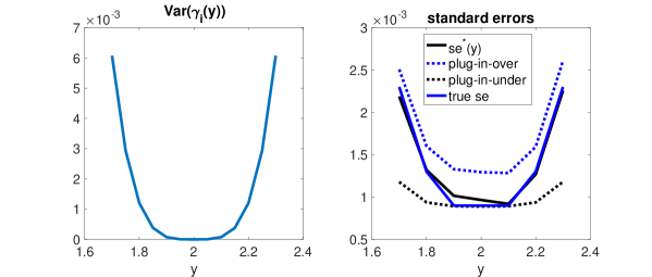
Figure 6.1. Left: $\mathsf{Var}(\gamma_{i}(y))$. Right: estimated and true standard errors of $\widehat{\theta}(y)$ for $y\in M$ in the dynamic DR model. In the right panel, we plot four “standard errors” for $y\in\mathcal{Y}$ under $N=T=300$. The true standard error is calculated as the standard deviation of $\widehat{\theta}(y)$ from 1,000 simulations, while the other three are calculated using a fixed simulation of data.

We examine the coverage properties of $\theta(y)$ and compare four inferential methods:

(i) Proposed: the proposed uniform inference procedure using the interquartile range described in Remark A.1.

(ii) No-debias: this method does not debias, while all other steps are the same as the proposed method.

(iii) Plug-in-over: this method plugs in the estimated standard error, it uses the estimated $V_{\psi}(y)$ and $V_{\gamma}(y)$ by:

$$\widehat{V}_{\psi}(y) = \frac{1}{N}\sum_{i=1}^{N}(S_{wz}^{\prime}\boldsymbol{w}_{i}\boldsymbol{w}_{i}^{\prime}S_{wz})\otimes\left[\widehat{\mathbb{A}}_{y,1i}\Xi(y)\widehat{\mathbb{A}}_{y,1i}\right].$$

$$\widehat{V}_{\gamma}(y) = \frac{1}{N}\sum_{i=1}^{N}(S_{wz}^{\prime}\boldsymbol{w}_{i}\boldsymbol{w}_{i}^{\prime}S_{wz})\otimes(\widehat{\gamma}_{i}(y)\widehat{\gamma}_{i}(y)^{\prime})$$

where computing the estimators $\widehat{\mathbb{A}}_{y,1i}$ and $\widehat{\gamma}_{i}(y)$ are straightforward. Meanwhile, we apply the Newey-West type estimator $\Xi(y)$ to estimate $\mathbb{E}(\frac{1}{T}\sum_{s,t\leq T}\psi_{it}(y_{k})\psi_{it}(y_{l})^{\prime}\mid W)$.

(iv) Plug-in-under: this method also plugs in the estimated standard error, but replaces $\widehat{\Sigma}_{NT}(y)$ of the Plug-in-over method with

$$\widetilde{\Sigma}_{NT}(y)=\frac{1}{NT}\widehat{V}_{\psi}(y).$$

Table 6.1 summarizes the coverage probabilities of $\{\theta(y):y\in{\mathcal{Y}}\}$ out of 1,000 replications. The results are generally as expected. The no-debias method performs unsatisfactorily when $T\leq N$ due to the incidental parameter bias issue. The plugin-over method assumes that there is arbitrary heterogeneity in $\beta_{i}(y)$, so is quite conservative; the plugin-under method is the standard treatment in the varying coefficient literature, which assumes that $\beta_{i}(y)$ is “explainable homogeneous” in the sense that it is fully captured by covariates $\boldsymbol{w}_{i}$. The confidence band resulting from $\widetilde{\Sigma}_{NT}(y)$ under covers $\theta(y)$.

Table 6.1. Coverage Probabilities of $\{\theta(y):y\in\mathcal{Y}\}$

		Methods
$T$	$N$	Proposed	No-debias	Plugin-over	Plugin-under
50	300	0.942	0.576	0.994	0.894
	400	0.945	0.440	0.998	0.899
100	300	0.946	0.813	0.995	0.854
	400	0.947	0.740	0.996	0.852
200	300	0.951	0.914	0.975	0.632
	400	0.958	0.883	0.970	0.621

7. Conclusion

We develop estimation and inference methods for dynamic distribution regression panel models that incorporate heterogeneity both within and between units. Our model can be employed in a large number of empirical settings. An empirical investigation of labor income processes illustrates some economic insights our approach can provide. We find that accounting for individual heterogeneity is important in studying the potential impact of income shocks on future income and evaluating how the income distribution responds to increases in the education levels of sub-populations of the data. Individual heterogeneity is also important in understanding income mobility and poverty persistence.

In the econometric analysis, the unknown degree of heterogeneity affects both the rate of convergence and the asymptotic distribution, making them unknown and continuously varying across different assumptions on the heterogeneity. While analytical plug-in methods for inference break down when the degree of heterogeneity varies, we prove that a simple cross-sectional bootstrap method is uniformly valid for a large class of data generating processes including the case of homogeneous coefficients.

We could extend our model in several directions. For instance, we could explicitly include time fixed effects and covariates with homogeneous coefficients in the first stage. This could be useful in empirical applications which directly model an outcome variable with trends rather than the residuals. To reduce the number of estimated parameters, we could model the individual coefficients in HDR using factor structures as in Chernozhukov et al. (2018b). We could also reduce dimensionality by modeling the between and within heterogeneity though a pseudo-factor structure where the value $y$ plays the role of time. For example, in the empirical application we can model the persistence coefficient as $\rho_{i}(y)\approx\boldsymbol{\lambda}_{i}^{\prime}\boldsymbol{f}_{y}$, where $\boldsymbol{\lambda}_{i}$ is a vector of loadings and $\boldsymbol{f}_{y}$ a vector of factors. Alternatively, we could use the grouped fixed effects approach of Bonhomme and Manresa (2015). Finally, while our focus here is a panel comprising repeated time series observations on the same unit our approach could be applied to a network setting in which there is contemporaneous dependence across units. We leave these extensions to future work.

Appendix A The bootstrap algorithms

In this section we introduce the bootstrap algorithm for confidence bands.

Algorithm A.1 (Confidence Band for Projections of Coefficients).

Step 0:

Pick the confidence level $p$, number of bootstrap repetitions $B$, region $\mathcal{Y}$ and a component of the linear projection. This amounts to selecting a vector $\boldsymbol{\eta}$ such that $\boldsymbol{\eta}^{\prime}\mathsf{vec}(\boldsymbol{\theta}(y))$ over $y\in\mathcal{Y}$ is the function of interest.

Step 1:

For any $y\in\mathcal{Y}$, obtain the debiased DR coefficient estimates

$$\widehat{\boldsymbol{\beta}}(y):=\{\widehat{\boldsymbol{\beta}}_{i}(y):i=1,...,N_{01}(y)\}$$

using (3.1), and the estimates of the linear projection, $\widehat{\boldsymbol{\theta}}(y)$, using (3.2).

Step 2:

For any $y\in\mathcal{Y}$, let $\{(\widehat{\boldsymbol{\beta}}_{i}^{*}(y),\boldsymbol{w}_{i}^{*},\boldsymbol{z}_{i}^{*}):i=1,...,N_{01}(y)\}$ be a random sample with replacement from $\{(\widehat{\boldsymbol{\beta}}_{i}(y),\boldsymbol{w}_{i},\boldsymbol{z}_{i}):i=1,...,N_{01}(y)\}$. Compute

$$\widehat{\boldsymbol{\theta}}^{*}(y)=\sum_{i=1}^{N_{01}(y)}\widehat{\boldsymbol{\beta}}^{*}_{i}(y)\widehat{\boldsymbol{z}}^{*}_{i}(y)^{\prime}\left(\sum_{i=1}^{N_{01}(y)}\widehat{\boldsymbol{z}}^{*}_{i}(y)\widehat{\boldsymbol{z}}^{*}_{i}(y)^{\prime}\right)^{-1}_{,}$$

$$\widehat{\boldsymbol{z}}^{*}_{i}(y):=\sum_{j=1}^{N_{01}(y)}\boldsymbol{z}^{*}_{j}\boldsymbol{w}_{j}^{*^{\prime}}\left(\sum_{j=1}^{N_{01}(y)}\boldsymbol{w}^{*}_{j}\boldsymbol{w}_{j}^{*^{\prime}}\right)^{-1}\boldsymbol{w}^{*}_{i}.$$

Step 3:

Repeat Step 2 for $B$ times to obtain $\{\widehat{\boldsymbol{\theta}}^{*}_{b}(y)\}_{b=1}^{B}$ for each $y\in\mathcal{Y}$.

Step 4:

Let $q_{\tau}$ be the booststrap $\tau$-quantile of

$$\left\{\sup_{y\in\mathcal{Y}}\left|\frac{\boldsymbol{\eta}^{\prime}\mathsf{vec}(\widehat{\theta}^{*}_{b}(y)-\widehat{\boldsymbol{\theta}}(y))}{s^{*}(y)}\right|\right\}_{b=1}^{B}$$

where $s^{*}(y)$ could be either the bootstrap standard deviation or rescaled interquartile range of $\{\boldsymbol{\eta}^{\prime}\mathsf{vec}(\widehat{\boldsymbol{\theta}}^{*}_{b}(y)\}_{b=1}^{B}$. See remark A.1 below.

Step 5:

Compute the asymptotic $p$-confidence band

$$\mathsf{CI}_{p}(\boldsymbol{\eta}^{\prime}\mathsf{vec}(\boldsymbol{\theta}(y))):=[\boldsymbol{\eta}^{\prime}\mathsf{vec}(\widehat{\boldsymbol{\theta}}(y))-q_{\tau}s^{*}(y),\boldsymbol{\eta}^{\prime}\mathsf{vec}(\widehat{\boldsymbol{\theta}}(y))+q_{\tau}s^{*}(y)].$$

Remark A.1 (Standard Errors).

We show in the appendix that the bootstrap standard deviation $s^{*}(y)$ is consistent, $(s^{*}(y)-\sigma(y))/\sigma(y)=o_{P}(1)$, uniformly in $y$, where $\sigma(y)=\sqrt{\boldsymbol{\eta}^{\prime}\Sigma_{NT}(y)\boldsymbol{\eta}}$. The bootstrap interquartile range rescaled with the standard normal distribution is an alternative: $s^{*}(y)=(q^{*}_{.75}(y)-q^{*}_{.25}(y))/(z_{.75}-z_{.25})$, where $q_{p}^{*}$ is the bootstrap $p$-quantile of $\boldsymbol{\eta}^{\prime}\mathsf{vec}(\widehat{\boldsymbol{\theta}}^{*}_{b}(y)-\widehat{\boldsymbol{\theta}}(y))$ and $z_{p}$ is the $p$-quantile of the standard normal. Our theory covers both cases.

For the actual and counterfactual distributions, it is convenient to express the estimator in (3.3) as

$$\widehat{G}_{t}(y)=\frac{1}{N}\sum_{i=1}^{N}\Psi_{i}(y;h(\boldsymbol{x}_{it}),\widehat{\boldsymbol{\beta}}^{g}_{i}(y))$$

with

$$\Psi_{i}(y;\boldsymbol{x},\boldsymbol{b}) = 1\{i\leq N_{01}(y)\}\Lambda(-\boldsymbol{x}^{\prime}\boldsymbol{b})+\frac{N_{1}(y)}{N}$$

$$-1\{i\leq N_{01}(y)\}\frac{1}{2T}\mathsf{tr}\left(\ddot{\Lambda}(-\boldsymbol{x}^{\prime}\boldsymbol{b})\boldsymbol{x}\boldsymbol{x}^{\prime}\widehat{\Sigma}_{i}(y)^{-1}\right),$$

to simplify the notation.

Algorithm A.2 (Confidence Band for Actual and Counterfactual Distribution).

Step 0:

Pick the confidence level $p$, number of bootstrap repetitions $B$, and region $\mathcal{Y}$.

Step 1:

For each $y\in\mathcal{Y}$, obtain the debised estimate $\widehat{G}_{t}$ from (3.3).

Step 2:

Let $\{(\boldsymbol{x}_{it}^{*},\widehat{\boldsymbol{\beta}}_{i}^{*}(y),\boldsymbol{w}_{i}^{*},\boldsymbol{z}_{i}^{*}):i=1,...,N_{01}(y)\}$ be a random sample with replacement from $\{(\boldsymbol{x}_{it},\widehat{\boldsymbol{\beta}}_{i}(y),\boldsymbol{w}_{i},\boldsymbol{z}_{i}):i=1,...,N_{01}(y)\}$. Compute

$$\widehat{G}^{*}_{t}(y)=\frac{1}{N}\sum_{i=1}^{N}\Psi_{i}(y;h_{it}(\boldsymbol{x}_{it}^{*}),\widehat{\boldsymbol{\beta}}_{i}^{g*}(y),\quad\widehat{\boldsymbol{\beta}}_{i}^{g*}(y)=\widehat{\boldsymbol{\beta}}^{*}_{i}(y)+\widehat{\boldsymbol{\theta}}^{*}(y)[g(\boldsymbol{z}_{i}^{*})-\boldsymbol{z}^{*}_{i}],$$

where $\widehat{\boldsymbol{\theta}}^{*}(y)$ is defined as in Step 2 of Algorithm A.1

Steps 3-5:

The same as Steps 3-5 of Algorithm A.1, with $(\widehat{G}^{*},\widehat{G})$ in place of $(\boldsymbol{\eta}^{\prime}\mathsf{vec}(\widehat{\boldsymbol{\theta}}^{*}),\boldsymbol{\eta}^{\prime}\mathsf{vec}(\widehat{\boldsymbol{\theta}}))$.

The bootstrap inference for the actual distribution $F_{t}(y)$ is a special case with $h(\boldsymbol{x}_{it})=\boldsymbol{x}_{it}$ and $g(\boldsymbol{z}_{i})=\boldsymbol{z}_{i}$. Finally, the algorithm below computes the confidence band for the quantile effects.

Algorithm A.3 (Confidence Bands for Quantile Effect).

Step 0:

Pick the confidence level $p$, number of bootstrap repetitions $B$, and region of quantile indexes $\mathcal{T}$.

Step 1:

For any $\tau\in\mathcal{T}$, obtain the estimate $\widehat{\mathsf{QE}}_{t}(\tau)$ using (3.6).

Step 2:

Compute the bootstrap draws of $\widehat{\mathsf{QE}}_{t}(\tau)$:

(1) Obtain $\widehat{F}_{t}^{*}$ and $\widehat{G}_{t}^{*}$ as in step 2 of Algorithm A.2. For $\widehat{F}_{t}^{*}$ , set $h(\boldsymbol{x}_{it})=\boldsymbol{x}_{it}$ and $g(\boldsymbol{z}_{i})=\boldsymbol{z}_{i}$.

(2) For any $\tau\in\mathcal{T}$, calculate

$$\widehat{\mathsf{QE}}^{*}_{t}(\tau)=\widetilde{\phi}(\widehat{G}^{*}_{t},\tau)-\widetilde{\phi}(\widehat{F}^{*}_{t},\tau).$$

Steps 3-5:

The same as Steps 3-5 of Algorithm A.1, with $(\widehat{\mathsf{QE}}_{t}^{*},\widehat{\mathsf{QE}}_{t})$ in place of $(\boldsymbol{\eta}^{\prime}\mathsf{vec}(\widehat{\theta}^{*}),\boldsymbol{\eta}^{\prime}\mathsf{vec}(\widehat{\theta}))$.

Remark A.2 (Computation).

The most computationally expensive task is the computation of coefficient estimates, which is conducted only in Step 1 of the algorithms.

Remark A.3 (Stationary Distributions and Effects).

The bootstrap algorithms for stationary distributions and quantile effects are omitted because their steps are similar to the corresponding steps in Algorithms A.2 and A.3.

References

- Arellano et al. (2017) Arellano, M., Blundell, R. and Bonhomme, S. (2017). Earnings and consumption dynamics: a nonlinear panel data framework. Econometrica 85 693–734.
- Arellano and Bond (1991) Arellano, M. and Bond, S. (1991). Some tests of specification for panel data: Monte carlo evidence and an application to employment equations. The Review of Economic Studies 58 277–297.
- Arellano and Bonhomme (2012) Arellano, M. and Bonhomme, S. (2012). Identifying distributional characteristics in random coefficients panel data models. The Review of Economic Studies 79 987–1020.
- Arellano and Hahn (2007) Arellano, M. and Hahn, J. (2007). Understanding bias in nonlinear panel models: Some recent developments. Econometric Society Monographs 43 381.
- Arellano and Weidner (2017) Arellano, M. and Weidner, M. (2017). Instrumental variable quantile regressions in large panels with fixed effects. Unpublished manuscript .
- Bonhomme and Manresa (2015) Bonhomme, S. and Manresa, E. (2015). Grouped patterns of heterogeneity in panel data. Econometrica 83 1147–1184.
- Champernowne (1953) Champernowne, D. G. (1953). A model of income distribution. The Economic Journal 63 318–351.
- Chen (2021) Chen, S. (2021). Quantile regression with group-level treatments. Working Paper.
- Chernozhukov et al. (2010) Chernozhukov, V., Fernández-Val, I. and Galichon, A. (2010). Quantile and probability curves without crossing. Econometrica 78 1093–1125.
- Chernozhukov et al. (2013) Chernozhukov, V., Fernández-Val, I. and Melly, B. (2013). Inference on counterfactual distributions. Econometrica 81 2205–2268.
- Chernozhukov et al. (2018a) Chernozhukov, V., Fernandez-Val, I. and Weidner, M. (2018a). Network and panel quantile effects via distribution regression. arXiv preprint:1803.08154 .
- Chernozhukov et al. (2018b) Chernozhukov, V., Hansen, C., Liao, Y. and Zhu, Y. (2018b). Inference for heterogeneous effects using low-rank estimation of factor slopes. arXiv preprint arXiv:1812.08089 .
- Chetverikov et al. (2016) Chetverikov, D., Larsen, B. and Palmer, C. (2016). Iv quantile regression for group-level treatments, with an application to the distributional effects of trade. Econometrica 84 809–833.
- Dhaene and Jochmans (2015) Dhaene, G. and Jochmans, K. (2015). Split-panel jackknife estimation of fixed-effect models. The Review of Economic Studies 82 991–1030.
- Fernández-Val (2009) Fernández-Val, I. (2009). Fixed effects estimation of structural parameters and marginal effects in panel probit models. Journal of Econometrics 150 71–85.
- Fernández-Val and Lee (2013) Fernández-Val, I. and Lee, J. (2013). Panel data models with nonadditive unobserved heterogeneity: Estimation and inference. Quantitative Economics 4 453–481.
- Fernández-Val and Weidner (2016) Fernández-Val, I. and Weidner, M. (2016). Individual and time effects in nonlinear panel models with large n, t. Journal of Econometrics 192 291–312.
- Fernández-Val and Weidner (2018) Fernández-Val, I. and Weidner, M. (2018). Fixed effects estimation of large-t panel data models. Annual Review of Economics 10 109–138.
- Foresi and Peracchi (1995) Foresi, S. and Peracchi, F. (1995). The conditional distribution of excess returns: An empirical analysis. Journal of the American Statistical Association 90 451–466.
- Galvao (2011) Galvao, A. (2011). Quantile regression for dynamic panel data with fixed effects. Journal of Econometrics 164 142–157.
- Galvao and Kato (2016) Galvao, A. and Kato, K. (2016). Smoothed quantile regression for panel data. Journal of Econometrics 193 92–112.
- Gonçalves and Kaffo (2015) Gonçalves, S. and Kaffo, M. (2015). Bootstrap inference for linear dynamic panel data models with individual fixed effects. Journal of Econometrics 186 407–426.
- Gu and Koenker (2017) Gu, J. and Koenker, R. (2017). Unobserved heterogeneity in income dynamics: An empirical bayes perspective. Journal of Business & Economic Statistics 35 1–16.
- Hahn and Kuersteiner (2011) Hahn, J. and Kuersteiner, G. (2011). Bias reduction for dynamic nonlinear panel models with fixed effects. Econometric Theory 27 1152–1191.
- Hahn and Newey (2004) Hahn, J. and Newey, W. (2004). Jackknife and analytical bias reduction for nonlinear panel models. Econometrica 72 1295–1319.
- Hamilton (2020) Hamilton, J. D. (2020). Time series analysis. Princeton university press.
- Hart (1976) Hart, P. E. (1976). The dynamics of earnings, 1963-1973. The Economic Journal 86 551–565.
- Hausman and Taylor (1981) Hausman, J. A. and Taylor, W. E. (1981). Panel data and unobservable individual effects. Econometrica: Journal of the Econometric society 1377–1398.
- Hirano (2002) Hirano, K. (2002). Semiparametric bayesian inference in autoregressive panel data models. Econometrica 70 781–799.
- Hsiao and Pesaran (2008) Hsiao, C. and Pesaran, M. H. (2008). Random coefficient models. In The econometrics of panel data. Springer, 185–213.
- Hu et al. (2019) Hu, Y., Moffitt, R. and Sasaki, Y. (2019). Semiparametric estimation of the canonical permanent-transitory model of earnings dynamics. Quantitative Economics 10 1495–1536.
- Kaffo (2014) Kaffo, M. (2014). Bootstrap inference for nonlinear dynamic panel data models with individual fixed effects. Tech. rep., mimeo.
- Kapetanios (2008) Kapetanios, G. (2008). A bootstrap procedure for panel data sets with many cross-sectional units. The Econometrics Journal 11 377–395.
- Kato et al. (2012) Kato, K., Galvao, A. F. and Montes-Rojas, G. V. (2012). Asymptotics for panel quantile regression models with individual effects. Journal of Econometrics 170 76–91.
- Koenker (2004) Koenker, R. (2004). Quantile regression for longitudinal data. Journal of Multivariate Analysis 91 74–89.
- Liao and Yang (2018) Liao, Y. and Yang, X. (2018). Uniform inference for characteristic effects of large continuous-time linear models .
- Lillard and Willis (1978) Lillard, L. A. and Willis, R. J. (1978). Dynamic aspects of earning mobility. Econometrica 46 985–1012.
- Lu and Su (2022) Lu, X. and Su, L. (2022). Uniform inference in linear panel data models with two-dimensional heterogeneity. Journal of Econometrics .
- Moffitt and Zhang (2018) Moffitt, R. and Zhang, S. (2018). Income volatility and the psid: Past research and new results. In AEA Papers and Proceedings, vol. 108.
- Mundlak (1978) Mundlak, Y. (1978). On the pooling of time series and cross section data. Econometrica: journal of the Econometric Society 69–85.
- Neyman and Scott (1948) Neyman, J. and Scott, E. (1948). Consistent estimates based on partially consistent observations. Econometrica 16 1–32.
- Nickell (1981) Nickell, S. J. (1981). Biases in dynamic models with fixed effects. Econometrica 49 1417–26.
- Okui and Yanagi (2019) Okui, R. and Yanagi, T. (2019). Panel data analysis with heterogeneous dynamics. Journal of Econometrics 212 451–475.
- Phillips and Moon (1999) Phillips, P. C. B. and Moon, H. (1999). Linear regression limit theory for nonstationary panel data. Econometrica 67 1057–1111.
- PSID (2020) PSID, I. f. S. R., Survey Research Center (2020). Panel study of income dynamics, public use dataset .
- Shorrocks (1976) Shorrocks, A. F. (1976). Income mobility and the markov assumption. The Economic Journal 86 566–578.
- Su et al. (2016) Su, L., Shi, Z. and Phillips, P. C. (2016). Identifying latent structures in panel data. Econometrica 84 2215–2264.
- Swamy (1970) Swamy, P. A. (1970). Efficient inference in a random coefficient regression model. Econometrica: Journal of the Econometric Society 311–323.
- Zhang et al. (2019) Zhang, Y., Wang, H. J. and Zhu, Z. (2019). Quantile-regression-based clustering for panel data. Journal of Econometrics 213 54–67.