The Rate-Distortion-Perception Tradeoff:
The Role of Common Randomness

Abstract

A rate-distortion-perception (RDP) tradeoff has recently been proposed by Blau and Michaeli and also Matsumoto. Focusing on the case of perfect realism, which coincides with the problem of distribution-preserving lossy compression studied by Li et al., a coding theorem for the RDP tradeoff that allows for a specified amount of common randomness between the encoder and decoder is provided. The existing RDP tradeoff is recovered by allowing for the amount of common randomness to be infinite. The quadratic Gaussian case is examined in detail.

I Introduction

Classical rate-distortion theory seeks reconstructions from rate-limited representations that are “close” to the original source realization in a specified sense. Closeness is conventionally measured via a single-letter distortion measure, i.e., that one depends only on the source and reconstruction realizations and that is additive over components of a string [1, 2, 3].

While broadly successful (e.g. [4, 5]), this approach does have certain limitations. One is that the reconstruction might be qualitatively quite different from the source realization that generated it. For an i.i.d. Gaussian source with mean-squared error (MSE) distortion measure, the reconstruction is generally of lower power than the source. For stationary Gaussian sources, the reverse waterfilling procedure [1] generally gives rise to reconstructions that have a null power spectrum at high frequencies. Thus JPEG images look blurry at low bit-rates.

Of course, all distortion measures used in theoretical studies of multimedia compression are proxies for the measure of real interest, namely how the reconstruction would be perceived by the (usually human) end-user. In some cases, this end-user will prefer a reconstruction that is more distorted according to conventional measures. For instance, in some cases, MPEG Advanced Audio Coding (ACC) populates high-frequency bands with artificial noise instead of leaving them null [5, Sec. 17.4.2], in order to match the power spectrum of the source; this is termed Perceptual Noise Substitution (PNS). This general idea has acquired renewed interest with the advent of neural-network-based image compressors, for which powerful discriminators [6, 7, 8] can be used to encourage the compression system to output images that are indistinguishable from naturally-occurring ones [9, 10, 11].

One way of capturing this notion mathematically is to require that the distribution of reconstructions be close, in some sense, to that of the source. Prior work has considered lossy compression under such a constraint [12, 13, 13, 14]. In particular, Li et al. [13] consider the informational quantity

$$R(\Delta) =\inf_{P_{Y|X}}I(X;Y)$$

$$\text{s.t.}\ E[D(X,Y)]\leq\Delta$$ (1)

$$\ \ \ \ \ Y\stackrel{{\scriptstyle d}}{{=}}X,$$

which they call the distribution preserving rate-distortion function (DP-RDF). More recently, Blau and Michaeli [15] and Matsumoto [16, 17] consider a more general version that constrains the divergence between the distributions of $X$ and $Y$ (see also [18]), the former calling it the rate-distortion-perception (RDP) function. We shall adopt the latter nomenclature, referring to the case in which $X\stackrel{{\scriptstyle d}}{{=}}Y$ as the perfect realism case. Both Li et al. and Blau and Michaeli provide a converse argument in support of (1). Li et al. provide an achievability argument in the Gaussian case. L. Theis and the author recently provided an operational formulation and an achievability result supporting the use of the RDP function [19] (see also [16]). That formulation is variable-rate and assumes infinite common randomness between the encoder and the decoder.

This paper provides a coding theorem for a fixed-rate scenario in which the amount of common randomness between the encoder and decoder is constrained. It turns out that the above RDP function only applies when the available common randomness is infinite. Thus, some care is required when interpreting (1) operationally.

The reason for characterizing the rate-distortion tradeoff as a function of the amount of common randomness available is not that common randomness is a costly resource in compression scenarios per se. Indeed, in practice the encoder can include a small seed for a pseudo-random number generator in its message. It could even use the compressed representation for one part of the source as the seed for another. Rather, we note that randomization is not necessary at all under conventional formulations of the problem: in a fixed-rated setting, if the distortion is the average of a function that only depends on the realizations of the source and the reconstruction, then in principle one could simply fix the realization of the common randomness to be one that minimizes this average. Note that the distortion measure in question could be quite complex, such as the median of the assessments of a collection of human subjects. Thus quantifying the amount of randomness that is needed under novel formulations is useful in that it illustrates how much they depart from conventional ones. The need for at least some common randomness has already been illustrated by Theis and Agustsson [22]. The precise characterization provided here has the benefit of establishing an intimate connection between distribution-preserving compression and distributed channel synthesis as studied by Cuff [23]. Indeed, the proof of our main result tracks that of [23, Theorem II.1].

II Results for General Sources

We are given a source distribution $P(x)$ over the alphabet $\mathcal{X}$ that is assumed i.i.d. when extended to sequences, and a distortion measure

$$D:\mathcal{X}\times\mathcal{X}\mapsto[0,\infty).$$ (2)

For a positive number $a$, let $[a]$ denote the set $\{1,\ldots,\lfloor a\rfloor\}$.

Definition 1.

An $(n,2^{nR},2^{nR_{c}})$ code consists of

1. a (privately randomized) encoder

   $$F:\mathcal{X}^{n}\times[2^{nR_{c}}]\mapsto[2^{nR}]$$ (3)

2. and a (privately randomized) decoder

   $$G:[2^{nR}]\times[2^{nR_{c}}]\mapsto\mathcal{X}^{n}.$$ (4)

Definition 2.

The triple $(R,R_{c},\Delta)$ is achievable with near-perfect (resp. perfect) realism if for all $\epsilon>0$, there exists a sequence of codes, $\{(F_{n},G_{n})\}_{n=1}^{\infty}$, the $n$th being $(n,2^{n(R+\epsilon)},2^{n(R_{c}+\epsilon)})$, such that eventually we have

$$E[D(X^{n},Y^{n})]\leq\Delta+\epsilon$$ (5)

and

$$d_{TV}(P_{X^{n}},P_{Y^{n}})\leq\epsilon,$$ (6)

(resp.

$$d_{TV}(P_{X^{n}},P_{Y^{n}})=0),$$ (7)

where $Y^{n}=G_{n}(F_{n}(X^{n},J),J)$ and $J$ is uniformly distributed over $[2^{n(R_{c}+\epsilon)}]$, independent of the source. Here $d_{TV}(\cdot,\cdot)$ refers to the total variation distance:

$$d_{TV}(P,Q)=\sup_{A}|P(A)-Q(A)|.$$ (8)

Our first result shows that any sequence of codes that achieves near-perfect realism can be upgraded to one that achieves perfect realism with no asymptotic change to the rates or the distortion. The result holds under the following assumption on the distortion measure and source distribution pair.

Definition 3.

A distortion measure and source distribution pair $(D,P)$ is uniformly integrable if for every $\epsilon>0$ there exists a $\delta>0$ such that

$$\sup_{X,Y,A}E[D(X,Y)\cdot 1_{A}]\leq\epsilon,$$ (9)

where the supremum is over all random variables $X$ and $Y$ having marginal distribution $P$ and all events $A$ such that $\Pr(A)\leq\delta$.

If $\mathcal{X}$ is finite then evidently any pair of distortion measure and source distribution is uniformly integrable. The quadratic Gaussian case is also uniformly integrable, since we have, by Cauchy-Schwarz,

$$E[(X-Y)^{2}1_{A}]\leq(\sqrt{E[X^{2}1_{A}]}+\sqrt{E[Y^{2}1_{A}]})^{2},$$ (10)

so since $X\stackrel{{\scriptstyle d}}{{=}}Y$,

$$\sup_{X,Y,A}E[(X-Y)^{2}1_{A}] \leq\sup_{A}4E[X^{2}1_{A}]$$ (11)

$$\leq 4\sqrt{E[X^{4}]\delta}$$ (12)

$$=4\sqrt{3\delta},$$ (13)

where we have used Cauchy-Schwarz for a second time.

Theorem 1.

If $(D,P)$ is uniformly integrable, then $(R,R_{c},\Delta)$ is achievable with perfect realism if and only if it is achievable with near-perfect realism.

Note that the proof does not rely on a single-letter characterization of the set of achievable rate-distortion triples.

Proof:

Suppose $(R,R_{c},\Delta)$ is achievable with near-perfect realism. Fix $\epsilon>0$ and choose $0<\delta<\epsilon/2$ such that

$$\sup_{X,Y,A}E[D(X,Y)\cdot 1_{A}]\leq\epsilon/2,$$ (14)

where the supremum is over $X$ and $Y$ with marginals $P$ and events $A$ with probability at most $\delta$. Let $(F_{n},G_{n})$ be a sequence of codes, the $n$th being $(n,2^{n(R+\delta)},2^{n(R_{c}+\delta)})$ such that eventually

$$E[D(X^{n},Y^{n})]\leq\Delta+\delta,$$ (15)

and

$$d_{TV}(P_{X^{n}},P_{Y^{n}})\leq\delta,$$ (16)

where $Y^{n}=G_{n}(F_{n}(X^{n},J),J)$. For fixed message $i$ and common randomness $j$, the privately randomized decoder $G_{n}$ can be viewed as a conditional distribution

$$W(y^{n}|i,j)\quad y^{n}\in\mathcal{X}^{n},i\in[2^{n(R+\delta)}],j\in[2^{n(R_{c}+\delta)}].$$ (17)

Let $PW(\cdot)$ denote the marginal distribution of the reconstruction induced by the encoder/decoder pair, i.e., for any event $A\subset\mathcal{X}^{n}$,

$$PW(A)=\sum_{i,j}\int_{\mathcal{X}^{n}}\frac{\Pr(F_{n}(x^{n},j)=i)}{2^{n(R_{c}+\delta)}}\;W(A|i,j)dP(x^{n}).$$ (18)

By hypothesis, we have

$$d_{TV}(PW(y^{n}),P(y^{n}))\leq\delta.$$ (19)

If the code does not already satisfy perfect realism, then we leave the encoder untouched and replace the decoder $G_{n}$ with one, say $\tilde{G}_{n}$, with the same rates, nearly the same distortion, and perfect realism, as follows.

Let $\Gamma(y^{n})$ denote a probability distribution over $\mathcal{X}^{n}$ with respect to which both $PW(y^{n})$ and $P(y^{n})$ are absolutely continuous (e.g., $(PW(y^{n})+P(y^{n}))/2$). Define the set

$$\mathcal{X}^{n}_{+}=\left\{y^{n}\in\mathcal{X}^{n}:\frac{dPW}{d\Gamma}(y^{n})>\frac{dP}{d\Gamma}(y^{n})\right\}.$$ (20)

and the parameters

$$\theta_{y^{n}}=\frac{dP/d\Gamma(y^{n})}{dPW/d\Gamma(y^{n})}\quad y^{n}\in\mathcal{X}_{+}^{n}.$$ (21)

For any indices $i$ and $j$ and any set $A$ in $\mathcal{X}^{n}$ the alternate decoder $\tilde{G}_{n}$ is defined via the conditional distribution

$$\tilde{W}(A|i,j)=\\ \int_{A\cap\mathcal{X}^{n}_{+}}\theta_{y^{n}}dW(y^{n}|i,j)+W(A\backslash\mathcal{X}^{n}_{+}|i,j)+\phi_{i,j}\cdot Q(A),$$ (22)

where the distribution $Q(y^{n})$ is defined as

$$Q(A)=\frac{\int_{A}(dP/d\Gamma(y^{n})-dPW/d\Gamma(y^{n}))^{+}d\Gamma(y^{n})}{\int(dP/d\Gamma(y^{n})-dPW/d\Gamma(y^{n}))^{+}d\Gamma(y^{n})}.$$ (23)

and the parameters $\phi_{i,j}$ are defined as

$$\phi_{i,j}=\int_{\mathcal{X}^{n}_{+}}(1-\theta_{y^{n}})dW(y^{n}|i,j).$$ (24)

One can verify by direct calculation that $\tilde{W}(\cdot|i,j)$ is a probability distribution for each $i$ and $j$ and moreover

$$P\tilde{W}(A) =\sum_{i,j}\int_{\mathcal{X}^{n}}\frac{\Pr(F_{n}(x^{n},j)=i)}{\lfloor 2^{n(R_{c}+\delta)}\rfloor}\;\tilde{W}(A|i,j)dP(x^{n})$$ (25)

$$=P(A)$$ (26)

as desired. Thus $(F_{n},\tilde{G}_{n})$ achieves perfect realism. Let $Y^{n}$ denote the output of $G_{n}$ and $\tilde{Y}^{n}$ the output of $\tilde{G}_{n}$. By (22), we have that for each $i,j$, the total variation distance satisfies

$$d_{TV}(W(\cdot|i,j),\tilde{W}(\cdot|i,j))\leq\phi_{i,j}.$$ (27)

Thus it is possible to couple $X^{n}$, $Y^{n}$, and $\tilde{Y}^{n}$ so that

$$\Pr(Y\neq\tilde{Y}|J=j,F_{n}(X^{n},J)=i)\leq\phi_{i,j}.$$ (28)

This in turn implies that

$$\Pr((X^{n},Y^{n})\neq(X^{n},\tilde{Y}^{n}))$$ (29)

$$=\sum_{i,j}\int_{\mathcal{X}^{n}}\frac{\Pr(F_{n}(x^{n},j)=i)}{\lfloor 2^{n(R_{c}+\delta)}\rfloor}\phi_{i,j}dP(x^{n})$$ (30)

$$=\sum_{i,j}\int_{\mathcal{X}^{n}}\int_{\mathcal{X}^{n}_{+}}\frac{\Pr(F_{n}(x^{n},j)=i)}{\lfloor 2^{n(R_{c}+\delta)}\rfloor}\left(1-\frac{\frac{dP}{d\Gamma}(y^{n})}{\frac{dPW}{d\Gamma}(y^{n})}\right)$$ (31)

$$\phantom{=\sum\int}dW(y^{n}|i,j)dP(x^{n})$$ (32)

$$=\sum_{i,j}\int_{\mathcal{X}^{n}}\int_{\mathcal{X}^{n}_{+}}\frac{\Pr(F_{n}(x^{n},j)=i)}{\lfloor 2^{n(R_{c}+\delta)}\rfloor}$$ (33)

$$\phantom{\sum\int}\frac{\frac{dPW}{d\Gamma}(y^{n})-\frac{dP}{d\Gamma}(y^{n})}{\frac{dPW}{d\Gamma}(y^{n})}dW(y^{n}|i,j)dP(x^{n})$$ (34)

$$=\int_{\mathcal{X}^{n}_{+}}\frac{\frac{dPW}{d\Gamma}(y^{n})-\frac{dP}{d\Gamma}(y^{n})}{\frac{dPW}{d\Gamma}(y^{n})}dPW(y^{n})$$ (35)

$$=\int_{\mathcal{X}^{n}_{+}}\left[\frac{dPW}{d\Gamma}(y^{n})-\frac{dP}{d\Gamma}(y^{n})\right]d\Gamma(y^{n})$$ (36)

$$=\int_{\mathcal{X}^{n}}\left[\frac{dPW}{d\Gamma}(y^{n})-\frac{dP}{d\Gamma}(y^{n})\right]^{+}d\Gamma(y^{n})$$ (37)

$$=d_{TV}(P(\cdot),PW(\cdot))$$ (38)

$$\leq\delta.$$ (39)

This fact can then be used to bound the distortion achieved by $(F_{n},\tilde{G}_{n})$

$$E[D(X^{n},\tilde{Y}^{n})] =\frac{1}{n}\sum_{i=1}^{n}E[D(X_{i},\tilde{Y}_{i})]$$ (40)

$$=\frac{1}{n}\sum_{i=1}^{n}E[D(X_{i},\tilde{Y}_{i})1_{\tilde{Y}_{i}=Y_{i}}]$$ (41)

$$\phantom{=E[}+\frac{1}{n}\sum_{i=1}^{n}E[D(X_{i},\tilde{Y}_{i})1_{\tilde{Y}_{i}\neq Y_{i}}]$$ (42)

$$\leq\Delta+\delta+\sup_{X,Y,A}E[D(X,Y)1_{A}]$$ (43)

$$\leq\Delta+\epsilon,$$ (44)

where the supremum is over all random variables $X$ and $Y$ having marginal distribution $P$ and all events $A$ such that $\Pr(A)\leq\delta$ and we have used (14), (15), and (16). ∎

Our main result is a characterization of the rate-distortion tradeoff with perfect (or near-perfect) realism and limited common randomness.

Definition 4.

$$\mathcal{RD}=\Big{\{}(R,R_{c},\Delta) :\ \text{there exists}\ (U,Y)\ \text{such that}$$ (45)

$$Y \stackrel{{\scriptstyle d}}{{=}}X$$ (46)

$$X \leftrightarrow U\leftrightarrow Y$$ (47)

$$R \geq I(X;U)$$ (48)

$$R_{c}+R \geq I(Y;U)$$ (49)

$$\Delta \geq E[D(X,Y)]\Big{\}}$$ (50)

Theorem 2.

If $(D,P)$ is uniformly integrable, then the triple $(R,R_{c},\Delta)$ is achievable with perfect realism (or near-perfect realism) iff it is contained in the closure of $\mathcal{RD}$.

Proof:

Note that the equivalence between perfect and near-perfect realism follows from the previous result. Suppose $(R,R_{c},\Delta)$ is achievable with perfect realism. Fix $\epsilon>0$, and let $(F_{n},G_{n})$ be a sequence of codes, the $n$th being $(n,2^{n(R+\epsilon)},2^{n(R_{c}+\epsilon)})$ eventually satisfying (5) and (7). Fix $n$ and let $I$ denote the message, i.e.,

$$I =F_{n}(X^{n},J)$$ (51)

$$Y^{n} =G_{n}(F_{n}(X^{n},J),J).$$ (52)

Let $T$ be uniformly distributed over $[n]$ and $U=(T,I,J)$. Then we have

$$n(R+\epsilon) \geq H(I)$$ (53)

$$\geq H(I|J)$$ (54)

$$\geq I(X^{n};I|J)$$ (55)

$$=I(X^{n};I,J)$$ (56)

$$=\sum_{i=1}^{n}I(X_{i};I,J,X^{i-1})$$ (57)

$$\geq\sum_{i=1}^{n}I(X_{i};I,J)$$ (58)

$$=nI(X_{T};I,J|T)$$ (59)

$$=nI(X_{T};U).$$ (60)

Similarly, since $Y^{n}\stackrel{{\scriptstyle d}}{{=}}X^{n}$,

$$n(R+R_{c}+2\epsilon) \geq H(I,J)$$ (61)

$$\geq I(Y^{n};I,J)$$ (62)

$$\geq\sum_{i=1}^{n}I(Y_{i};I,J)$$ (63)

$$\geq nI(Y_{T};I,J|T)$$ (64)

$$\geq nI(Y_{T};U).$$ (65)

Evidently we have $X_{T}\leftrightarrow U\leftrightarrow Y_{T}$, $X_{T}\stackrel{{\scriptstyle d}}{{=}}Y_{T}\stackrel{{\scriptstyle d}}{{=}}X$. It is straightforward to verify that

$$E[D(X_{T},Y_{T})]\leq\Delta+\epsilon.$$ (66)

It follows that if $(R,R_{c},\Delta)$ is achievable with perfect realism then it is within $\epsilon$ of $\mathcal{RD}$ for any $\epsilon>0$.

For achievability, it suffices to show that $(R,R_{c},\Delta)$ in the closure of $\mathcal{RD}$ is achievable with near-perfect realism, by Theorem 1. Fix $\epsilon>0$ and $(U,Y)$ satisfying

$$R+\epsilon >I(X;U)$$ (67)

$$R_{c}+R+2\epsilon >I(Y;U)$$ (68)

$$\Delta+\epsilon >E[D(X,Y)]$$ (69)

and $X\leftrightarrow U\leftrightarrow Y$ and $Y\stackrel{{\scriptstyle d}}{{=}}X$. Let $P(x,u,y)$ denote the joint distribution of these variables. Consider selecting a random codebook $U^{n}(i,j)$ for $i\in[2^{n(R+\epsilon)}]$, $j\in[2^{n(R_{c}+\epsilon)}]$ i.i.d. $P(u)$. By the soft covering lemma [23, Lemma IV.1], (see also [24, 25, 26]) and (68) we have

$$\lim_{n\rightarrow\infty}E\left[d_{TV}\left(P_{Y^{n}},\sum_{i,j}\frac{P_{Y^{n}|U^{n}}(\cdot|U^{n}(i,j))}{\lfloor 2^{n(R+\epsilon)}\rfloor\lfloor 2^{n(R_{c}+\epsilon)}\rfloor}\right)\right]=0,$$ (70)

and by (67)

$$\lim_{n\rightarrow\infty}\frac{1}{2^{n(R_{c}+\epsilon)}}\sum_{j}E\left[d_{TV}\left[P_{X^{n}},\sum_{i}\frac{P_{X^{n}|U^{n}}(\cdot|U^{n}(i,j))}{\lfloor 2^{n(R+\epsilon)}\rfloor}\right]\right]$$

$$\phantom{\lim 2^{n(R_{c}+\epsilon}}=0.$$ (71)

At the same time, by the law of large numbers, we have

$$\sum_{i,j}\int\int\frac{D(x^{n},y^{n})dP_{X^{n},Y^{n}|U^{n}}(x^{n},y^{n}|U^{n}(i,j))}{\lfloor 2^{n(R+\epsilon)}\rfloor\lfloor 2^{n(R_{c}+\epsilon)}\rfloor}\\ \stackrel{{\scriptstyle P}}{{\rightarrow}}E[D(X,Y)].$$ (72)

Thus for all sufficiently large $n$, there exists a realization of the code, $\{u^{n}(i,j)\}_{i,j}$, satisfying

$$d_{TV}\left(P_{Y^{n}}(\cdot),\sum_{i,j}\frac{P_{Y^{n}|U^{n}}(\cdot|u^{n}(i,j))}{\lfloor 2^{n(R+\epsilon)}\rfloor\lfloor 2^{n(R_{c}+\epsilon)}\rfloor}\right) <\epsilon,$$ (73)

$$\frac{1}{\lfloor 2^{n(R_{c}+\epsilon)}\rfloor}\sum_{j}d_{TV}\left(P_{X^{n}}(\cdot),\sum_{i}\frac{P_{X^{n}|U^{n}}(\cdot|u^{n}(i,j))}{\lfloor 2^{n(R+\epsilon)}\rfloor}\right) <\epsilon,$$ (74)

and

$$\sum_{i,j}\int\int\frac{D(x^{n},y^{n})dP_{X^{n},Y^{n}|U^{n}}(x^{n},y^{n}|u^{n}(i,j))}{\lfloor 2^{n(R+\epsilon)}\rfloor\lfloor 2^{n(R_{c}+\epsilon)}\rfloor}\\ \leq\Delta+\epsilon.$$ (75)

Let $Q_{X^{n},Y^{n},I,J}$ denote the joint distribution

$$Q_{X^{n},Y^{n},I,J}(x^{n},y^{n},i,j)=\\ \frac{1}{\lfloor 2^{n(R+\epsilon)}\rfloor\lfloor 2^{n(R_{c}+\epsilon)}\rfloor}P_{X^{n},Y^{n}|U^{n}}(x^{n},y^{n}|u^{n}(i,j)),$$ (76)

and note that we have, eventually,

$$d_{TV}(P_{Y^{n}},Q_{Y^{n}}) <\epsilon$$ (77)

$$\frac{1}{\lfloor 2^{n(R_{c}+\epsilon)}\rfloor}\sum_{j=1}^{\lfloor 2^{n(R_{c}+\epsilon)}\rfloor}d_{TV}(P_{X^{n}},Q_{X^{n},J}(\cdot|j)) <\epsilon,$$ (78)

$$E_{Q}[D(X^{n},Y^{n})] <\Delta+\epsilon.$$ (79)

Given a source string $x^{n}$ and a realization $j$ of the common randomness, the encoder selects a message $i\in[2^{n(R+\epsilon)}]$ randomly, using private randomness, with probability

$$Q_{I|X^{n},J}(i|x^{n},j),$$ (80)

assuming $Q(x^{n},j)>0$. Otherwise, it selects a message at random. The decoder creates $Y^{n}$ by passing $u^{n}(i,j)$ through the i.i.d. channel $P_{Y^{n}|U^{n}}$. The resulting joint distribution is given by

$$dP_{X}(x^{n})\frac{1}{\lfloor 2^{n(R_{c}+\epsilon)}\rfloor}Q_{I|X^{n},J}(i|x^{n},j)dP_{Y^{n}|U^{n}}(y^{n}|u^{n}(i,j)),$$ (81)

which we denote by $\tilde{Q}(\cdot)$. Now from (77)-(78) we have that eventually (cf. Cuff [23, Eqs. (61) and (64)])

$$d_{TV}(Q,\tilde{Q})<\epsilon.$$ (82)

It follows by (77) and the triangle inequality for total variation distance that the code achieves near-perfect realism. At the same time, by (82),

$$E_{\tilde{Q}}[D(X^{n},Y^{n})]-E_{Q}[D(X^{n},Y^{n})]\leq\sup_{X,Y,A}E[D(X,Y)1_{A}]$$ (83)

where the supremum is over $X$ and $Y$ with marginal $P$ and event $A$ with probability at most $\epsilon$. The conclusion then follows from (79) and the uniform integrability assumption. ∎

The fact that we need only consider perfect realism allows us to sidestep the continuity argument in the proof of [23, Thm. II.1], which in turn allows us to establish the converse for general spaces.

The two extreme cases of Theorem 2 are notable. Formally substituting $R_{c}=\infty$ into $\mathcal{RD}$ yields the region in (1). With no common randomness, the region is different.

Corollary 1 (No Common Randomness).

The triple $(R,0,\Delta)$ is achievable iff $(R,\Delta)$ is contained in the closure of the set

$$\mathcal{RD}_{0}=\Big{\{}(R,\Delta) :\ \text{there exists}\ (U,Y)\ \text{such that}$$ (84)

$$Y \stackrel{{\scriptstyle d}}{{=}}X$$ (85)

$$X \leftrightarrow U\leftrightarrow Y$$ (86)

$$R \geq\max(I(X;U),I(U;Y))$$ (87)

$$\Delta \geq E[D(X,Y)]\Big{\}}.$$ (88)

Proof:

Evidently we have

$$\mathcal{RD}_{0}=\{(R,\Delta):(R,0,\Delta)\in\mathcal{RD}\},$$ (89)

and thus

$$\operatorname*{cl}(\mathcal{RD}_{0}) =\operatorname*{cl}\{(R,\Delta):(R,0,\Delta)\in\mathcal{RD}\}$$ (90)

$$\subseteq\{(R,\Delta):(R,0,\Delta)\in\operatorname*{cl}(\mathcal{RD})\},$$ (91)

where $\operatorname*{cl}(\cdot)$ denotes closure. Achievability then follows from Theorem 2. Conversely, if $(R,0,\Delta)$ is achievable, then for all $\epsilon>0$, $(R+\epsilon,\epsilon,\Delta+\epsilon)\in\mathcal{RD}$. This implies that $(R+2\epsilon,0,\Delta+\epsilon)\in\mathcal{RD}$ and hence $(R+2\epsilon,\Delta+\epsilon)\in\mathcal{RD}_{0}$, since the encoder can simply transmit some of its private randomness to the decoder. It follows that $(R,\Delta)\in\operatorname*{cl}(\mathcal{RD}_{0})$. ∎

The quadratic Gaussian case, to which we turn next, illustrates the difference between these two cases.

III The Quadratic Gaussian Case

Proposition 1.

If the source $X$ is standard Normal and $D(x,y)=(x-y)^{2}$, then for $0<\Delta\leq 2$, $(R,R_{c},\Delta)$ is achievable iff

$$R\geq\frac{1}{2}\log_{2}\frac{1}{1-\rho^{2}},$$ (92)

where $\rho$ is the unique solution in $[0,1)$ to

$$1-\frac{\Delta}{2}=\rho\sqrt{1-2^{-2R_{c}}(1-\rho^{2})}.$$ (93)

Taking $R_{c}\rightarrow\infty$ gives $R\geq\frac{1}{2}\log_{2}\frac{1}{\Delta(1-\Delta/4)}$, which was previously derived by Li et al. [13, Prop. 2]. On the other hand, taking $R_{c}=0$ gives $R\geq\frac{1}{2}\log_{2}\frac{1}{\Delta/2}$, which is consistent with the finding of Theis and Agustsson [22] and Blau and Michael [18] for general sources that, under a mean squared error distortion constraint and in the absence of common randomness, imposing perfect realism incurs a 3 dB penalty compared to the case without a realism constraint. Fig. 1 illustrates the rate-distortion tradeoff for $R_{c}=0$, $R_{c}\rightarrow\infty$, and the classical case with no realism constraint [27, Sec. 10.3.2]. Note that at small distortions, requiring perfect realism incurs essentially no rate penalty, assuming infinite common randomness is available.

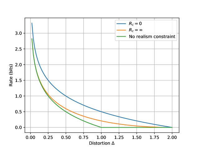
Figure 1: Rate-distortion tradeoffs for a Gaussian source with mean-squared error distortion for $R_{c}=0$, $R_{c}\rightarrow\infty$, and the classical rate-distortion function without a realism constraint.

Proof:

Since the source and distortion are uniformly integrable, we can apply Theorem 2. Given $\rho$ satisfying (93), choose $U$ to be standard Normal so that $X\leftrightarrow U\leftrightarrow Y$ are jointly Gaussian and

$$E[XU] =\rho$$ (94)

$$E[UY] =\sqrt{1-2^{-2R_{c}}(1-\rho^{2})}=:\tilde{\rho}$$ (95)

with $Y$ also being standard Normal. Then we have

$$E[(X-Y)^{2}] =E[(X-\rho U+\rho U-\tilde{\rho}U+\tilde{\rho}U-Y)^{2}]$$ (96)

$$=E[(X-\rho U)^{2}]+\phantom{}$$ (97)

$$\phantom{=E[(}E[(\rho U-\tilde{\rho}U)^{2}]+E[(\tilde{\rho}U-Y)^{2}]$$ (98)

$$=1-\rho^{2}+(\rho-\tilde{\rho})^{2}+1-\tilde{\rho}^{2}$$ (99)

$$=2-2\rho\tilde{\rho}$$ (100)

$$=2-2\rho\sqrt{1-2^{-2R_{c}}(1-\rho^{2})}$$ (101)

$$=\Delta$$ (102)

and

$$I(X;U) =\frac{1}{2}\log_{2}\frac{1}{1-\rho^{2}}$$ (103)

$$I(Y;U) =\frac{1}{2}\log_{2}\frac{1}{1-\tilde{\rho}^{2}}$$ (104)

$$=\frac{1}{2}\log_{2}\frac{1}{2^{-2R_{c}}(1-\rho^{2})}$$ (105)

$$=R_{c}+\frac{1}{2}\log_{2}\frac{1}{1-\rho^{2}}.$$ (106)

Thus the condition $R+R_{c}\geq I(Y;U)$ is equivalent to $R\geq I(X;U)$. Achievability then follows from Theorem 2.

To show the reverse direction, suppose $(R,R_{c},\Delta)$ is achievable. Then for all $\epsilon>0$, $(R+\epsilon,R_{c}+\epsilon,\Delta+\epsilon)\in\mathcal{RD}$ and there exists $(U,Y)$ satisfying

$$Y \stackrel{{\scriptstyle d}}{{=}}X$$ (107)

$$X \leftrightarrow U\leftrightarrow Y$$ (108)

$$R+\epsilon >I(X;U)$$ (109)

$$R_{c}+R+2\epsilon >I(Y;U)$$ (110)

$$\Delta+\epsilon >E[(X-Y)^{2}].$$ (111)

Now define

$$\rho =\sqrt{E[E[X|U]^{2}]}$$ (112)

$$\tilde{\rho} =\sqrt{E[E[Y|U]^{2}]}.$$ (113)

Then we have

$$R+\epsilon \geq I(X;U)$$ (114)

$$=h(X)-h(X|U)$$ (115)

$$\geq h(X)-h(X-E[X|U])$$ (116)

$$\geq\frac{1}{2}\log_{2}(2\pi e)-\frac{1}{2}\log_{2}(2\pi eE[(X-E[X|U])^{2}])$$ (117)

$$=\frac{1}{2}\log_{2}\frac{1}{E[(X-E[X|U])^{2}]}$$ (118)

$$=\frac{1}{2}\log_{2}\frac{1}{1-E[E[X|U]^{2}]}$$ (119)

$$=\frac{1}{2}\log_{2}\frac{1}{1-\rho^{2}},$$ (120)

where we have used the entropy-maximizing property of the Gaussian distribution. Similarly,

$$R+R_{c}+2\epsilon\geq I(Y;U)\geq\frac{1}{2}\log_{2}\frac{1}{1-\tilde{\rho}^{2}},$$ (121)

which reduces to

$$R+2\epsilon\geq\frac{1}{2}\log_{2}\frac{2^{-2R_{c}}}{1-\tilde{\rho}^{2}}.$$ (122)

Turning to the distortion constraint,

$$\Delta+\epsilon \geq E[(X-Y)^{2}]$$ (123)

$$=E[(X-E[X|U])^{2}]+E[(E[X|U]-E[Y|U])^{2}]$$ (124)

$$\phantom{=E[(}+E[(E[Y|U]-Y)^{2}]$$ (125)

$$\geq(1-\rho^{2})+(1-\tilde{\rho}^{2})+\phantom{}$$ (126)

$$\phantom{\geq(1-}\left(\sqrt{E[E[X|U]^{2}]}-\sqrt{E[E[Y|U]^{2}]}\right)^{2}$$

$$=(1-\rho^{2})+(1-\tilde{\rho}^{2})+(\rho-\tilde{\rho})^{2}$$ (127)

$$=2-2\rho\tilde{\rho},$$ (128)

where the second inequality follows from Cauchy-Schwarz. Thus we have

$$R+2\epsilon \geq\inf_{\rho,\tilde{\rho}\in[0,1)}\max\left(\frac{1}{2}\log_{2}\frac{1}{1-\rho^{2}},\frac{1}{2}\log_{2}\frac{2^{-2R_{c}}}{1-\tilde{\rho}^{2}}\right)$$ (129)

s.t. $$\Delta+\epsilon\geq 2-2\rho\tilde{\rho}.$$ (130)

We can assume $\Delta+\epsilon<2$, since the $\Delta=2$ case is trivial. Then at optimality, we must have

$$\frac{1}{2}\log_{2}\frac{1}{1-\rho^{2}}=\frac{1}{2}\log_{2}\frac{2^{-2R_{c}}}{1-\tilde{\rho}^{2}},$$ (131)

i.e.,

$$\tilde{\rho}=\sqrt{1-2^{-2R_{c}}(1-\rho^{2})}.$$ (132)

The conclusion then follows by taking $\epsilon\rightarrow 0$. ∎

References

- [1] T. Berger, Rate Distortion Theory: A Mathematical Basis for Data Compression. Englewood Cliffs, NJ: Prentice Hall, 1971.
- [2] C. E. Shannon, “A mathematical theory of communication,” Bell Syst. Tech. J., vol. 27, pp. 379–423 and 623–656, 1948.
- [3] ——, “Coding theorems for a discrete source with a fidelity criterion,” IRE Nat. Conv. Rec., vol. 7, no. 4, pp. 142–163, Mar. 1959.
- [4] W. A. Pearlman and A. Said, Digital Signal Compression: Principles and Practice. Cambridge University Press, 2011.
- [5] K. Sayood, Introduction to Data Compression, 4th ed. Morgan Kaufmann, 2012.
- [6] I. J. Goodfellow, J. Pouget-Abadie, M. Mirza, B. Xu, D. Warde-Farley, S. Ozair, A. Courville, and Y. Bengio, “Generative adversarial nets,” in Proc. Adv. Neural Inf. Proc. Sys. (NeurIPS).
- [7] M. Arjovsky, S. Chintala, and L. Bottou, “Wasserstein generative adversarial networks,” in Proc. Intl. Conf. Mach. Learn. (ICML), vol. 70, 2017, pp. 214–223.
- [8] I. Gulrajani, F. Ahmed, M. Arjovsky, V. Dumoulin, and A. Courville, “Improved training of Wasserstein GANs,” in Proc. Adv. Neural Inf. Proc. Sys. (NeurIPS), 2017.
- [9] M. Tschannen, E. Agustsson, and M. Lucic, “Deep generative models for distribution-preserving lossy compression,” in Proc. Adv. Neural Inf. Proc. Sys. (NeurIPS), 2018.
- [10] O. Rippel and L. Bourdev, “Real-time adaptive image compression,” in Proc. Intl. Conf. Mach. Learn. (ICML), 2017, pp. 2922–2930.
- [11] E. Agustsson, M. Tschannen, F. Mentzer, R. Timofte, and L. Van Gool, “Generative adversarial networks for extreme learned image compression,” in Proc. IEEE Conf. Comp. Vision, 2019, pp. 221–231.
- [12] E. J. Delp and O. R. Mitchell, “Moment preserving quantization,” IEEE Trans. Commun., vol. 37, no. 11, pp. 1549–1558, Nov. 1991.
- [13] M. Li, J. Klejsa, and W. B. Kleijn, “On distribution preserving quantization.” [Online]. Available: https://arxiv.org/abs/1108.3728
- [14] M. Li, J. Klejsa, A. Ozerov, and W. B. Kleijn, “Audio coding with power spectral density preserving quantization,” in IEEE Conf. Acoust., Speech, and Sig. Proc., 2012, pp. 413–416.
- [15] Y. Blau and T. Michaeli, “Rethinking lossy compression: The rate-distortion-perception tradeoff,” in Proc. Intl. Conf. Mach. Learn. (ICML), vol. 97, 2019.
- [16] R. Matsumoto, “Introducing the perception-distortion tradeoff into the rate-distortion theory of general information sources,” IEICE Comm. Express, vol. 7, no. 11, pp. 427–431, 2018.
- [17] ——, “Rate-distortion-perception tradeoff of variable-length source coding for general information sources,” IEICE Comm. Express, vol. 8, no. 2, pp. 38–42, 2019.
- [18] Y. Blau and T. Michaeli, “The perception-distortion tradeoff,” in Proc. IEEE Conf. Comp. Vision and Pattern Recog. (CVPR), 2018, pp. 6288–6237.
- [19] L. Theis and A. B. Wagner, “A coding theorem for the rate-distortion-perception function,” in Neural Compression: From Information Theory to Applications – Workshop @ ICLR 2021, 2021.
- [20] A. B. Wagner and J. Ballé, “Neural networks optimally compress the sawbridge,” in Proc. Data Comp. Conf. (DCC), 2021, pp. 143–152.
- [21] A. György and T. Linder, “Optimal entropy-constrained scalar quantization of a uniform source,” IEEE Trans. Inf. Theory, vol. 46, no. 7, pp. 2704–2711, 2000.
- [22] L. Theis and E. Agustsson, “On the advantages of stochastic encoders,” in Neural Compression: From Information Theory to Applications – Workshop @ ICLR 2021, 2021.
- [23] P. Cuff, “Distributed channel synthesis,” IEEE Trans. Inf. Theory, vol. 59, no. 11, pp. 7071–7096, 2013.
- [24] A. D. Wyner, “The common information of two dependent random variables,” IEEE Trans. Inf. Theory, vol. 21, no. 2, pp. 163–179, 1975.
- [25] T. S. Han and S. Verdú, “Approximation theory of output statistics,” IEEE Trans. Inf. Theory, vol. 39, no. 3, pp. 752 – 772, 1993.
- [26] M. Hayashi, “General nonasymptotic and asymptotic formulas in channel resolvability and identification capacity and their application to the wiretap channel,” IEEE Trans. Inf. Theory, vol. 52, no. 4, pp. 1562–1575, 2006.
- [27] T. M. Cover and J. A. Thomas, Elements of Information Theory, 2nd ed. Hoboken: John Wiley & Sons, 2006.
- [28] A. B. Wagner, “The rate-distortion-perception tradeoff: Perfect realism with randomized codes,” in Proc. IEEE Int. Symp. Inf. Theory (ISIT), 2022, submitted. [Online]. Available: arXiv
- [29] G. Zhang, J. Qian, J. Chen, and A. Khisti, “Universal rate-distortion-perception representations for lossy compression,” in Proc. Adv. Neural Inf. Proc. Sys. (NeurIPS), 2021.